DatasetEquity: Are All Samples Created Equal?
In The Quest For Equity Within Datasets

Abstract

Data imbalance is a well-known issue in the field of machine learning, attributable to the cost of data collection, the difficulty of labeling, and the geographical distribution of the data. In computer vision, bias in data distribution caused by image appearance remains highly unexplored. Compared to categorical distributions using class labels, image appearance reveals complex relationships between objects beyond what class labels provide. Clustering deep perceptual features extracted from raw pixels gives a richer representation of the data. This paper presents a novel method for addressing data imbalance in machine learning. The method computes sample likelihoods based on image appearance using deep perceptual embeddings and clustering. It then uses these likelihoods to weigh samples differently during training with a proposed Generalized Focal Loss function. This loss can be easily integrated with deep learning algorithms. Experiments validate the method’s effectiveness across autonomous driving vision datasets including KITTI and nuScenes. The loss function improves state-of-the-art 3D object detection methods, achieving over 200% AP gains on under-represented classes (Cyclist) in the KITTI dataset. The results demonstrate the method is generalizable, complements existing techniques, and is particularly beneficial for smaller datasets and rare classes. Code is available at: https://github.com/towardsautonomy/DatasetEquity

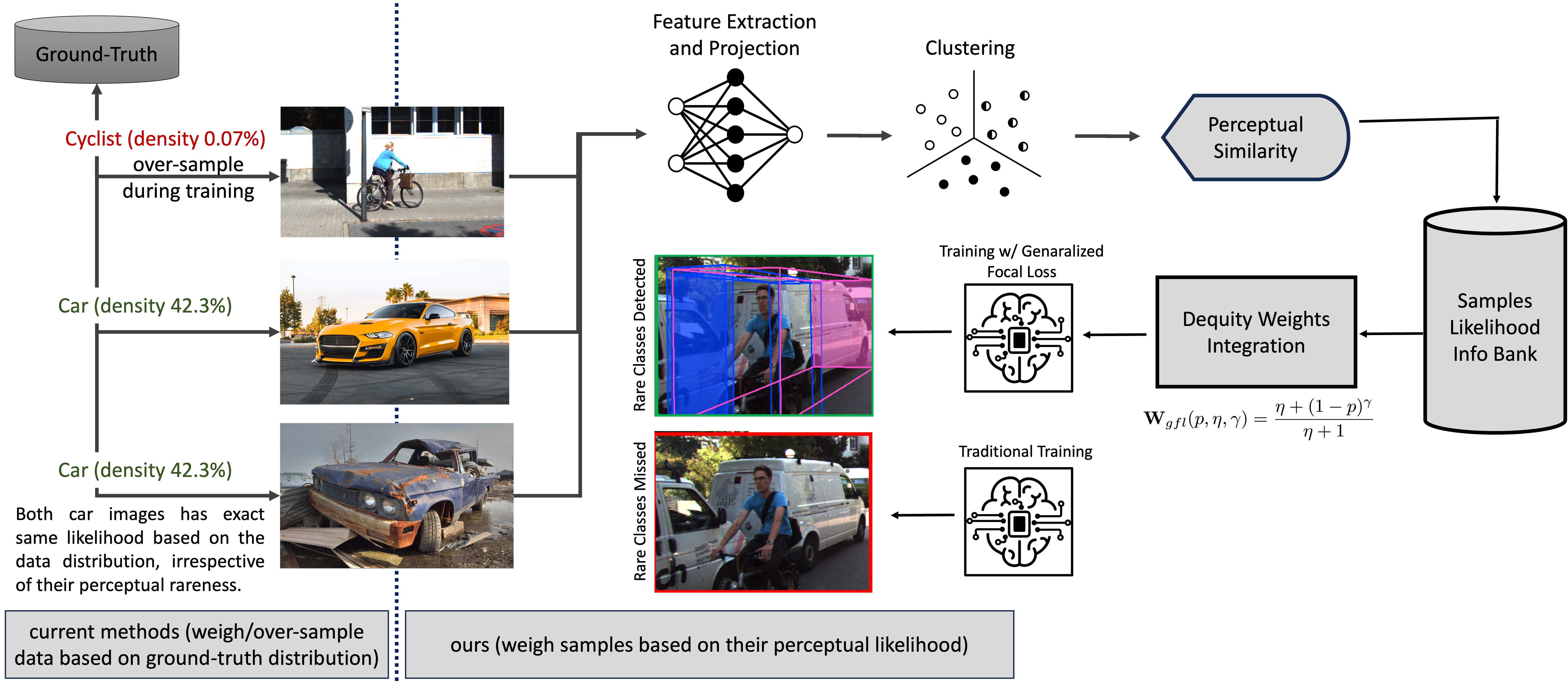
Figure 1: Left: existing techniques requiring class distribution annotations. Right: our method does not have ground truth dependencies. This work presents a method to estimate sample likelihoods by clustering semantic embeddings of raw image pixels. This enables modeling of visual relationships and data heterogeneity without reliance on categorical labels. The computed likelihoods are used to reweight training losses via a proposed Generalized Focal Loss function. Experiments demonstrate improved performance on rare and out-of-distribution samples in autonomous driving datasets. Compared to traditional training and results (red box), our method trained with generalized focal loss can successfully detect rare classes like van and cyclist (green box).

1 Introduction

Current methods for tackling data imbalance in machine learning either use some sort of Importance Weighting [4], or weigh the loss based on model prediction confidence for classification [26]. The problem of dataset bias as understood in the literature for tasks such as object detection only refers to the imbalance in the class of objects such as car, pedestrian, cyclist, or high level features like lighting and shadow conditions [50, 22]. They rely on class distribution, however do not consider perceptual feature likelihood as a way of understanding the data distribution. This is problematic, as class labels do not encapsulate fine-grained details like an object’s context, occlusion, resolution, etc. Weighting by image likelihood captures these nuances missed by class information alone. This a dataset that was collected 70% in NYC and 30% in the Mojave Desert with equal class distribution will still have a huge dataset imbalance, and without this information available as a part of dataset metadata, it will be impossible to account for with existing methods. Furthermore, our proposed method does not require a labeled dataset and rather operates on raw data samples, making it applicable to unsupervised techniques such as DINO [7] for computer vision tasks.

Existing work in computer vision literature considers all samples to be equally important and defines objective functions without considering how likely it is to occur within a given dataset. If we instead weighed errors for less likely samples higher than more likely samples, it would encourage the model to put more attention on those samples, thereby ‘equalizing’ the scales for all data samples.

The proposed method tackles data imbalance via: (1) Image embeddings are extracted for each sample using a pre-trained model, mapping them to a high-dimensional feature space; (2) These embeddings are clustered together based on appearance similarity, grouping frames with similar visual characteristics; (3) The relative size of each cluster indicates the likelihood of samples in that cluster occurring in the dataset. These likelihoods are then utilized to reweight training losses. By first embedding frames into a perceptual feature space and clustering based on image semantics, we can estimate sample occurrence probabilities without relying on class labels. Reweighting the loss function by these computed likelihoods helps address imbalances in the visual data distribution.

The main contributions of this work are:

1. A novel framework to prepare sample likelihoods information bank by clustering semantic embeddings of raw pixels. Unlike class-based techniques, this captures inter-object relationships and data heterogeneity missed by categorical labels alone.

2. Introduction of novel Generalized Focal Loss that reweights by computed likelihoods, improving modeling of rare and OOD classes.

3. State-of-the-art results on major autonomous driving benchmarks, with over 200% AP gains on rare classes like cyclist.

4. Ablations demonstrating generalizability across datasets and complementarity to class-based techniques.

5. Open source code to enable further research into image-based likelihoods for mitigating dataset bias. By looking beyond class labels to raw pixels, this work opens promising new directions. .

2 Related Work

Class-Based Resampling: Class-based resampling involves either oversampling the under-represented classes or undersampling the over-represented classes in order to balance the data distribution [2]. This can be achieved by a variety of methods, such as generating synthetic data for the under-represented classes [20], randomly selecting a subset of the over-represented classes, or randomly duplicating examples in minority classes. However, this may be problematic and may increase the likelihood of overfitting [15]. Region-Proposal-Network (RPN) [34] based architecture also suffers from class imbalance problem because of a large number of easy negatives, and a common solution is to perform some form of hard negative mining [42, 44, 11, 35].

Confidence-Based Weighing: The idea behind confidence-based weighing is to encourage the model to put more emphasis on samples that are difficult to classify, thereby reducing the impact of data imbalance on the model’s performance. It has been applied to a variety of tasks, such as object detection and image classification. One example of confidence-based weighing is focal loss [26], which modifies the standard cross-entropy loss function by adding a scaling factor that down-weights the loss for well-classified samples. This encourages the model to focus on difficult samples to classify, improving its performance on imbalanced data.

Other methods for confidence-based weighing have also been proposed, such as dynamically weighted balanced loss [12] and class-balanced loss [9, 45]. These methods have shown promising results for addressing data imbalance in various tasks.

Image Embeddings for Dataset Analysis: Image embeddings are a powerful tool for understanding the distribution of data in a dataset. They are a mathematical representation of an image in a high-dimensional space, where similar images are mapped to nearby points. Image embeddings can be used for dataset analysis by first extracting the embeddings for each image in the dataset using a pre-trained model. These embeddings can then be clustered together using unsupervised learning techniques, such as DBSCAN clustering, to group similar-looking images. The relative sizes of these clusters provide insight into the distribution of the data, allowing for the identification of any bias or imbalance in the dataset [1, 19, 13].

Image-Based 3D Object Detection: Recent advances in computer vision have led to the development of image-based 3D object detection methods, which use only camera images as input in autonomous driving. These methods are typically based on a Convolutional Neural Network (CNN) [37, 31, 38] or a combination of CNN and Transformers [25, 48] to process the images and predict the 3D location and orientation of objects in the scene. For 3D bounding-box predictions, either the perspective view or a learned mapping from the perspective view to Bird’s Eye View (BEV) [25, 28, 18, 51] representation of the scene is used. Several methods have been proposed to improve further the accuracy of 3D object detection, including the use of depth information [37, 31], multiple cameras [25, 28, 18, 51], temporal information [25, 51], and multiple modalities [28, 24, 30, 36].

3 Methodology

The first step in enforcing dataset equity is understanding whether or not bias exists within the dataset based on sample appearance. Once we have determined that, some level of bias quantification is required to attempt combating this particular type of bias. In the following sections, we first build an intuition for this kind of dataset bias in autonomous driving datasets and then propose a way of quantifying it in Section 3.2. The design of a loss function to tackle such dataset biases is further discussed in Section 3.3 which allows us to boost performance on under-represented samples for camera-based 3D object detection tasks.

3.1 Dataset Description

In this work, two challenging autonomous driving datasets have been used to conduct our experiments with computer vision tasks: (1) nuScenes [5], and (2) KITTI [14] object detection dataset. We also analyze additional datasets such as WaymoOpenDataset [41], and BDD100K [49], to demonstrate further the type of biases that exists and attempts to quantify it.

KITTI dataset: KITTI 3D object detection benchmark is one of the most popular autonomous driving benchmarks and consists of $7481$ training samples, and $7518$ testing samples. KITTI dataset provides no validation set, however, it is common practice to split the training data into $3712$ training and $3769$ validation images as proposed in [8], and then report validation results. This benchmark consists of $8$ different classes but evaluates only $3$ classes: car, pedestrian, and cyclist. The evaluation metric is the mean average precision (mAP) in 3D and Birds-Eye View (BEV) space, using a class-specific threshold on Intersection-over-Union (IoU). The average precision is computed using $41$ recall points ($AP|_{40}$) [39]. The objects in the various splits are organized into three partitions according to their difficulty level (easy, moderate, hard), and are evaluated separately.

nuScenes dataset: nuScenes [5]contains $1000$ driving scenes of 20s duration with keyframes annotated at 2Hz. Collected in Boston and Singapore, Collected across Boston and Singapore, it includes $28130$ training, $6019$ validation, and $6008$ test images from $6$ cameras. For 3D object detection, nuScenes provides 1.4M manually annotated boxes over $23$ classes. The official evaluation metric is nuScenes detection score (NDS), which aggregates mean average precision (mAP) and true positive errors for translation, scale, orientation, velocity, and attributes. NDS provides a holistic measure, unlike the mAP-based KITTI metric.

Waymo Open Dataset: Waymo Open Dataset [41] has been introduced to the autonomous driving research community as a large-scale, high-quality, diverse dataset, which consists of $1150$ scenes that each span 20 seconds, across a range of conditions in multiple cities. The dataset is curated to resolve the lack of the environments variations. The geographical area covered in Waymo Open Dataset is larger than other autonmous driving datasets [5] [49] [14], in terms of distribution of the coverage across geographies.

BDD100K dataset: BDD100K [49] is a diverse driving video dataset with $100,000$ videos and annotation information for $10$ computer vision tasks. The dataset is designed to help train and evaluate models for autonomous driving applications. It includes a wide range of environments, including urban, and rural scenes, and covers various weather conditions, lighting conditions, and time of day.

3.2 Dataset Analysis

In order to understand the data distribution, it is imperative to have some sense of similarity or distance between data samples. Image feature embeddings in a lower-dimensional space are extracted to compute the distance between two image frames. These features are then clustered together; the relative size of each cluster then gives us a sense of probabilities for samples within the given cluster occurring within the dataset.

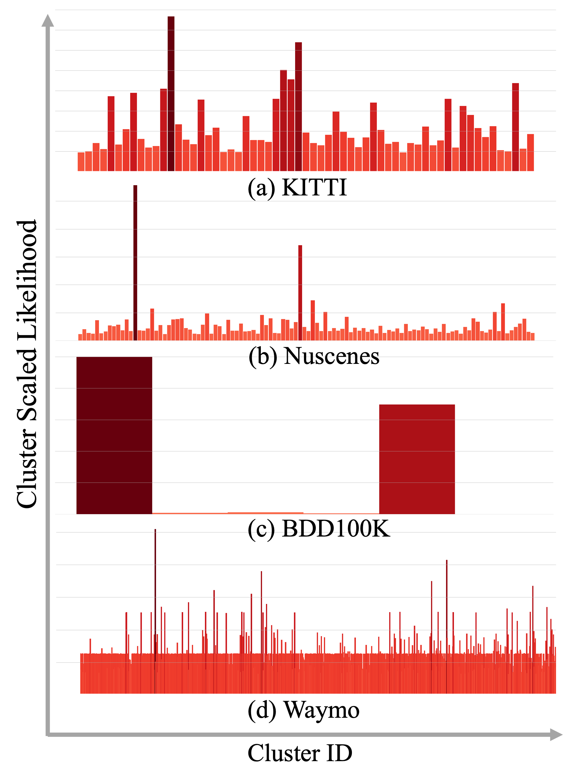
Figure 2: To analyze dataset bias, this work extracts CLIP [33] embeddings of raw pixels and clusters them with HDBSCAN [29] to discover non-uniform sample likelihoods. Unlike existing techniques relying on categorical labels, this captures visual relationships in an unsupervised manner. The derived likelihoods are then utilized to reweight loss functions, improving model performance on rare and out-of-distribution data.

Datasets considered in this work are: (1) nuScenes [5], and (2) KITTI object [14] (3) WaymoOpenDataset [41], and (4) BDD100K [49]. For all of these datasets, each image sample from the front camera in the training set is passed through a pre-trained network such as ResNet101 [16] or CLIP [32], to obtain the image embedding, which is a lower-dimensional vector summarizing image semantics and appearance.

Embedding from every image sample within the dataset is further projected onto a much lower-dimensional (3-dimensional) t-SNE [43] space and then clustered together using algorithms like DBSCAN [10] or Hierarchical DBSCAN [6]. t-SNE has shown to be effective for clustering applications, and as demonstrated by the authors of [27], the early exaggeration phase can be leveraged as a powerful clustering tool that mimics the behavior of spectral clustering. Thus, in this paper, we use t-SNE as a pre-processing step before applying the clustering method to separate clusters in lower dimensions to both reduce the computation cost, and improve the clustering results.

Cluster size and the total number of samples in the training dataset are then used to compute the cluster likelihood of occurring within that dataset. This is a good representative of each sample likelihood within that cluster. This likelihood is computed as:

$$P({C_{i}})=\frac{|C_{i}|}{N}$$ (1)

Where $C_{i}$ refers to the $i^{th}$ cluster, $|C_{i}|$ is the number of samples in $i^{th}$ cluster, and $N$ is the total number of samples within the training dataset.

These probabilities could be significantly low depending on the size of the training set. We, however, seek to compute probabilities relative to the largest cluster. This can be achieved by rewriting equation 1 as 2, and then setting the scale factor $\tilde{K}=1.0$ to compute cluster likelihood as shown in equation 3. This effectively gives us a relative likelihood of each cluster with respect to the largest cluster of data samples.

$$\begin{split}P({C_{i}})&=\frac{|C_{i}|}{N}\frac{\max_{i}(|C_{i}|)}{\max_{i}(|C_{i}|)}=\frac{|C_{i}|}{\max_{i}(|C_{i}|)}\tilde{K}\end{split}$$ (2)

$$\mathcal{L}_{s^{(i)}}=\frac{|C_{i}|}{\max_{i}(|C_{i}|)}$$ (3)

$\mathcal{L}_{s^{(i)}}$ in equation 3 is the scaled likelihood of samples corresponding to $i^{th}$ cluster. Histogram of these cluster likelihoods are shown in Figure 2.

3.3 Generalized Focal Loss

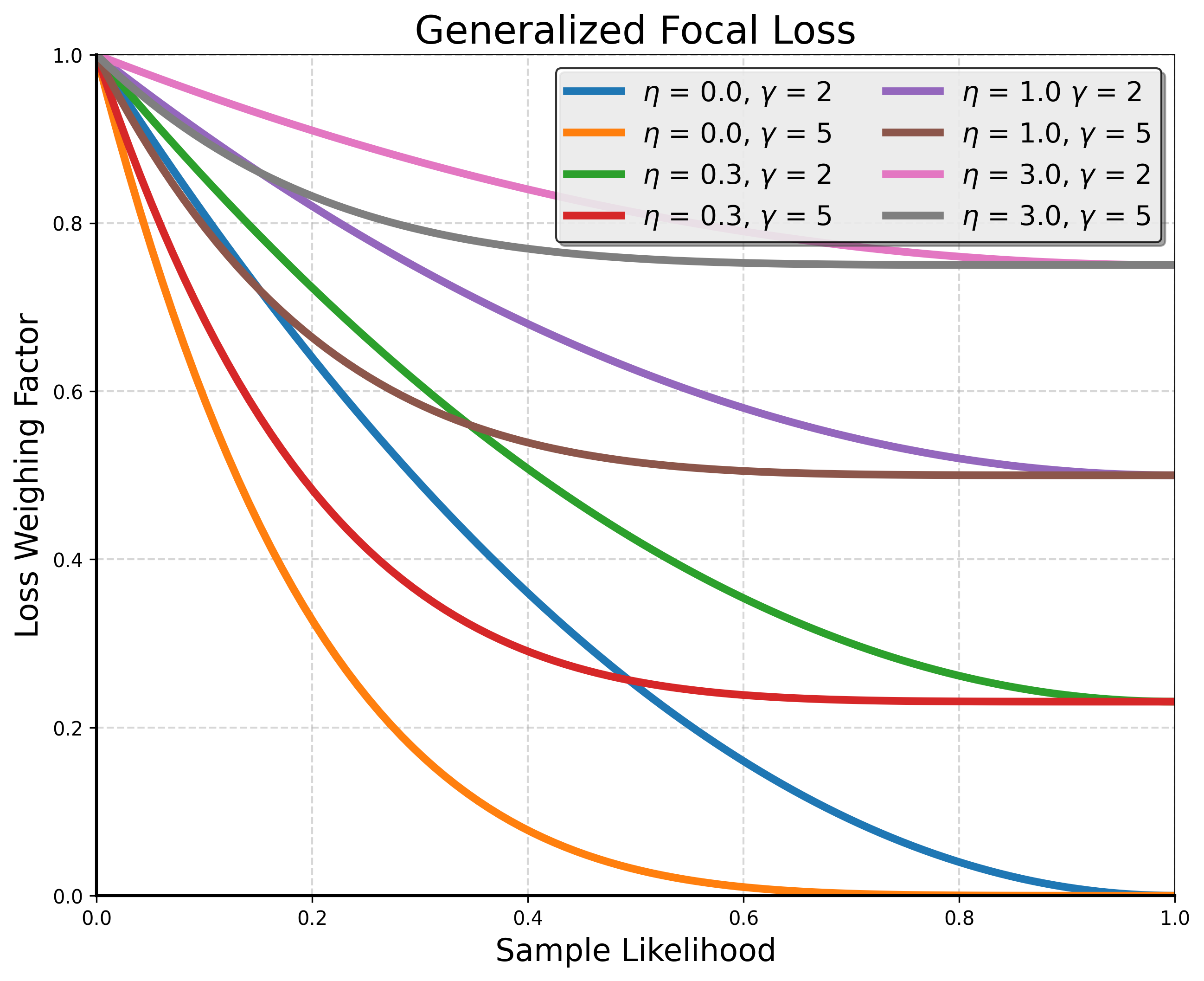
Figure 3: We propose a novel loss function called Generalized Focal Loss, which addresses the issue of data imbalance in computer vision by weighting each sample differently based on its likelihood of occurrence, leading to improved performance on downstream computer vision tasks. Plot of this function for various $\eta$ and $\gamma$ is shown in this figure; note that it defaults to Focal Loss for $\eta=0.0$.

Knowledge of sample likelihoods allows us to weigh each sample loss differently, thereby enforcing dataset equity. A new loss weighting function called Generalized Focal Loss as given in equation 4 is designed, which helps push the losses for less-likely samples high, and vice versa. Plots for this function against sample likelihood for various $\eta$ and $\gamma$ are shown in Figure 3. Note that, for $\eta=0$, this function defaults to Focal Loss [26] weighting function.

$$\mathbf{W}_{gfl}(p,\eta,\gamma)=\frac{\eta+(1-p)^{\gamma}}{\eta+1}$$ (4)

This way of training neural networks for computer vision tasks is described in Figure 1. Please note that we do not propose to replace Focal Loss with our loss, but rather to use them in conjunction, and we demonstrate these added benefits on baseline methods - all of which already use focal loss during the training process.

3.4 Camera-Based 3D Object Detection

This work takes camera-based 3d object detection as an example task to demonstrate the effectiveness of our proposed method. To test our method’s generalizability, we conduct experiments on 3 existing methods, namely, BEVFormer [25], DD3D [31], and BEVFusion [28], across two datasets - nuScenes, and KITTI. These two methods are chosen because they are state-of-the-art for camera-based 3d object detection tasks on the two datasets and have their implementations publicly available. During the training, Generalized Focal Loss weight is computed for each sample and is multiplied to the total loss before backward propagation. This does not increase the number of parameters of the model, and only adds a single $multiplication$ node in the computational graph during backpropagation without affecting the inference time of the underlying tasks. This simple method of sample reweighing improves the mAP score of DD3D by over $200\%$ for under-represented classes of KITTI dataset, the mAP score of BEVFormer by $1.44\%$ on nuScenes dataset, and the mAP score of BevFusion camera-only model by $1.05\%$ on nuScenes dataset. Note that although applying on same nuscenes dataset, BEVFormer and BevFusion share different model architecture, and our method achieves consistent improvements over both models.

Improvements with our methods are truly apparent for samples with low-likelihood, such as a camera frame containing object classes with very few instances within dataset, or common objects with partial occlusion/rare appearance. This is demonstrated in Figure 6(f). Comparison of validation graphs during training also hints at the advantage of using our loss function on under-represented samples. While there does not seem to be much advantage for a well-represented object class such as car, on pedestrian classes the model seems to be converging quickly while achieving higher AP as shown in Figure 4.

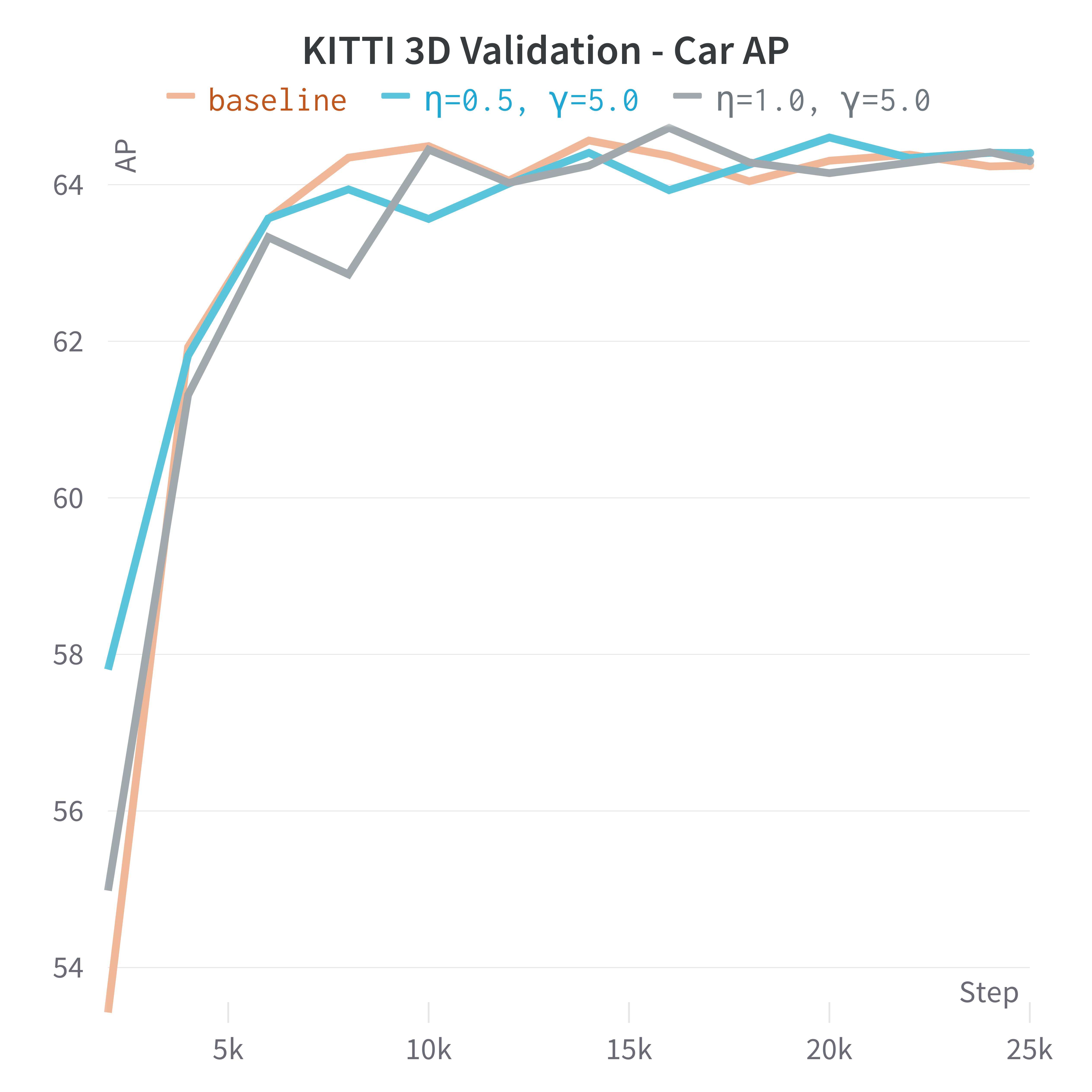
(a)

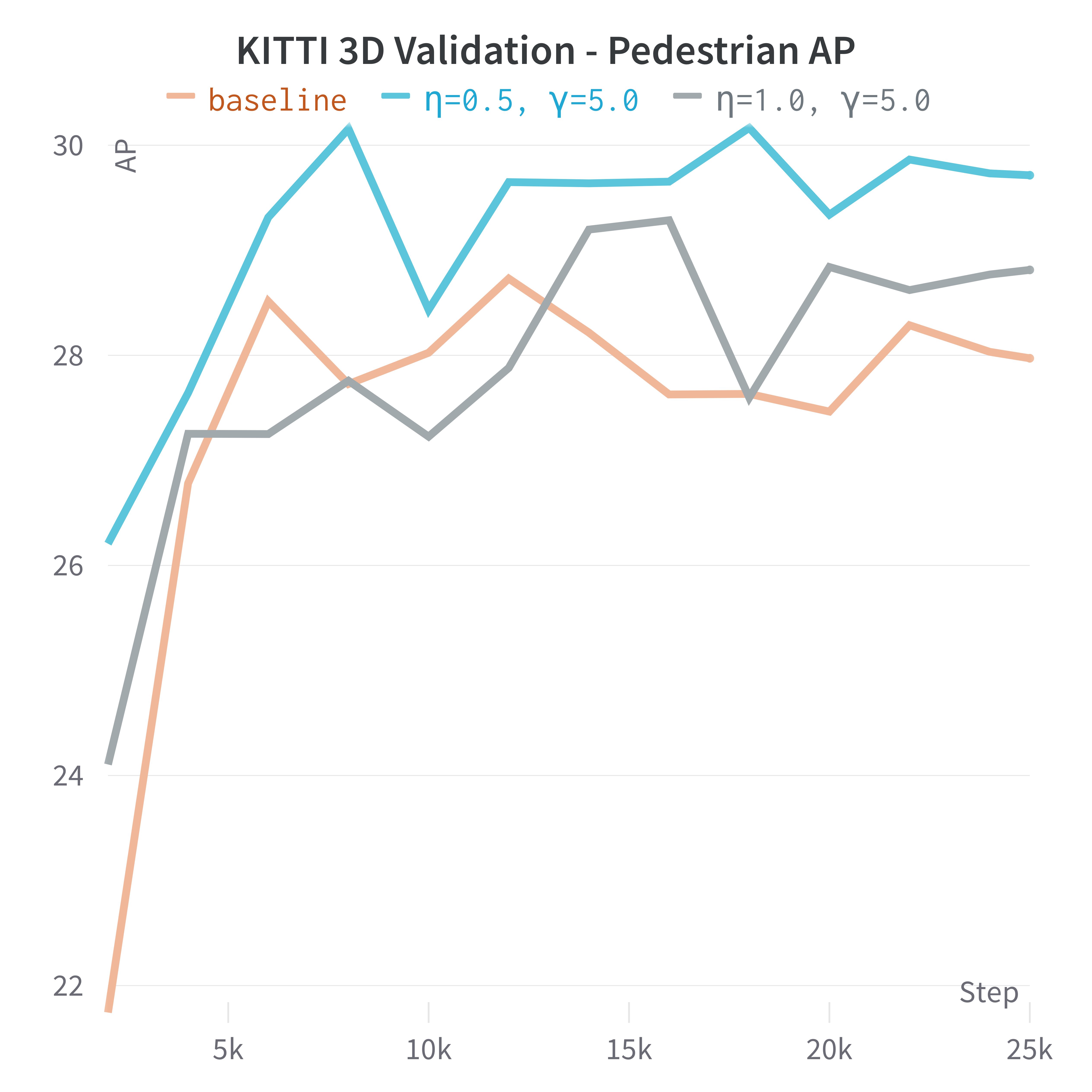
(b)

Figure 4: Validation AP for car and pedestrian during training as a function of number of optimization steps. Model trained with the Generalized Focal Loss achieves higher AP quickly on under-represented object classes, such as pedestrian in the KITTI 3D object dataset.

For BEVFormer, we train the BEVFormer-base and BEVFormer-small variants on the nuScenes training dataset, and test it on both, $validation$, as well as $test$ split. DD3D, which is state-of-the-art for monocular 3D object detection on KITTI dataset, has been trained in two different modes, (1) the model is trained on the train split and tested on val split, and (2) the model is trained on the trainval split and tested on the test set on KITTI server. For BEVFusion baseline, the camera-only model has been trained from scratch on the nuScenes training dataset, and validated on the nuScenes val dataset. More details about the experiments are given in Section 4.

4 Experimental Section

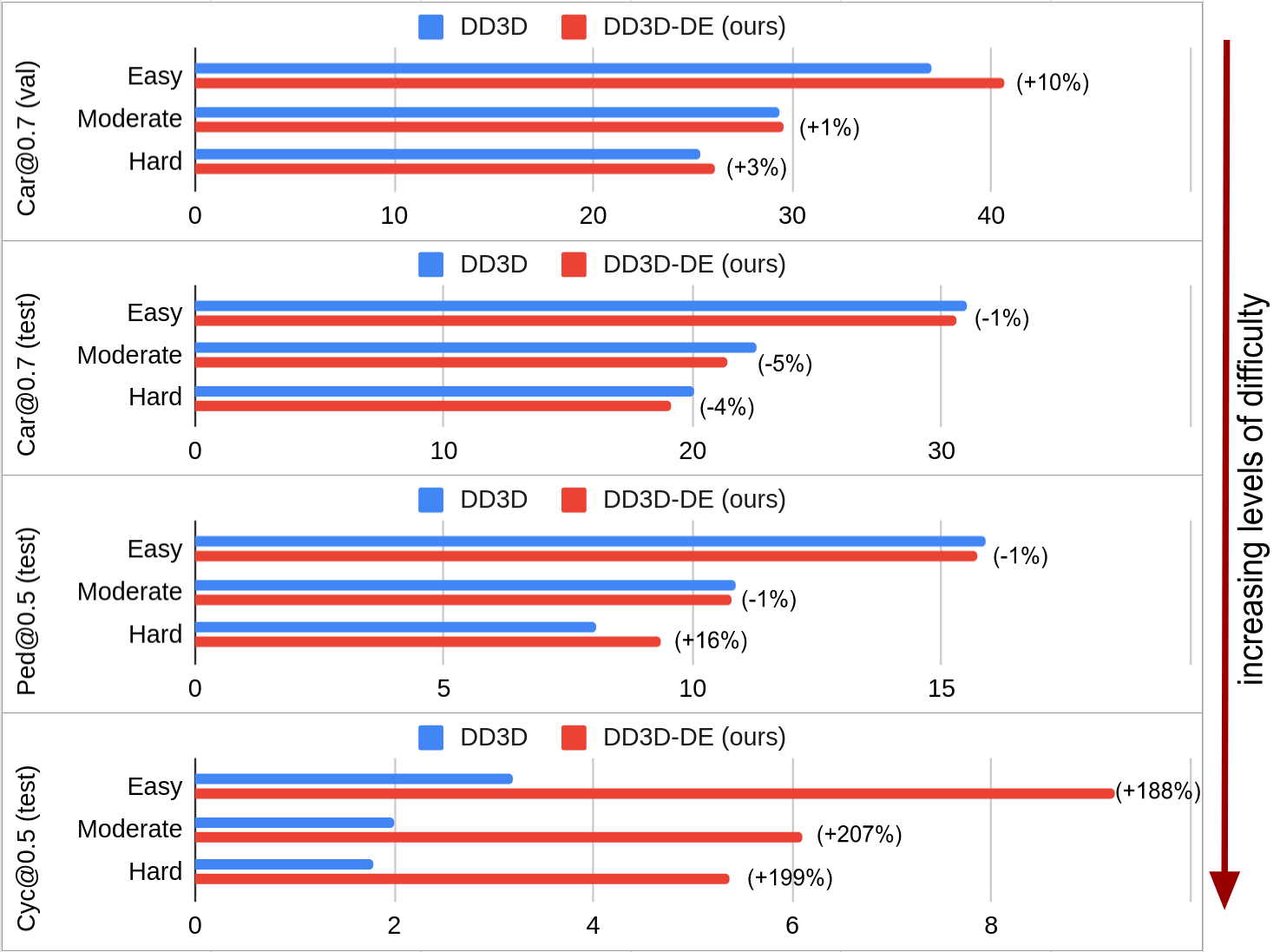
Figure 5: Comparison of BEV AP for a camera-based 3D object detection method called DD3D, with and without the proposed Generalized Focal Loss function, showing a significant improvement in performance when using the proposed loss function, particularly as the difficulty of the problem increases. Levels of difficulty here refer to the object class rareness, and within each object class, easy, moderate, and hard add another level of hierarchy. The use of the Generalized Focal Loss function brings equity within datasets and equalizes scales for all samples.

To further validate the effectiveness of our loss function on different model architectures, three methods of camera-based 3D object detection on two different AV datasets have been benchmarked. While our method only improve performance of BEVFormer and BEVFusion models on the nuScenes benchmarking dataset by only about $1\%$, the improvement on KITTI dataset is substantial ( $10\%$ improvement on val set), especially for the under-represented classes such as pedestrian, and cyclist, achieving over $200\%$ gain in mAP. This could be due to size of KITTI dataset is much smaller compared to the nuScene dataset and has a huge discrepancy in terms of class distribution in Table 1.

In addition, we suspect that existing dataset balancing technique such as Class-balanced Grouping and Sampling(CBGS)[52] has played critical role on models trained with nuscenes, thus further experiments has been conducted in Table 6 that excludes the impact of CBGS, and  $10\%$ improvement in NDS has been observed on our BEVFusion model. This shows the impact of considering features of a whole scene while sampling/weight balancing compared to label based sampling. For all datasets, features extracted from samples are first projected down onto a $3D$ t-SNE[43] space initialized with PCA[21], which is then followed by either DBSCAN[10], or HDBSCAN[6] algorithm for feature clustering to quantify sample likelihoods. Parameters used for clustering were $[\epsilon=2.0,\texttt{min\_samples=10}]$ for KITTI, $[\epsilon=1.0,\texttt{min\_samples}=10]$ for nuScenes, $[\epsilon=1.0,\texttt{min\_samples=10}]$ for WaymoOpenDataset, and $[\epsilon=1.5,\texttt{min\_samples=100}]$ for BDD100K.

Table 1: Distribution of class instances in KITTI object training dataset across 5 categories.

Category	Car	Pedestrian	Van	Cyclist	Truck
# Instances	28742	4487	2914	1627	1094

DD3D: V2-99 [23] extended to an FPN was used to train the DD3D model on KITTI dataset. Quantitative results of the model trained with our loss function on val set and test set are shown in Tables 2 and 3 respectively. We split the data into train and val set as described in 3.1, train the model on train set, and report the results on val set. For reporting the results on test split, we train on the entire trainval split, and then submit our predictions on test split to the KITTI server for benchmarking. Qualitative analysis of the improvements brought by our method over the baseline DD3D is demonstrated in Figure 6(f), which clearly illustrates how the Generalized Focal Loss really shines for methods working with datasets where all samples might not be equally likely. These models were trained for a total of $25000$ steps with a batch size of $24$, on a single NVIDIA A100 GPU. Initial learning rate of $0.002$, with MultiStepLR scheduler was used during training .

Table 2: 3D detection results on KITTI val set. The suffix DE signifies our method of applying Generalized Focal Loss weights to each sample. The best results are highlighted in bold. Class@N in this table refers to the $AP|_{R40}$ score computed for Class at an IoU threshold of $N$.

Methods	$\eta$	$\gamma$	Car@0.7
			BEV AP
			Easy	Mod	Hard
DD3D	-	-	37	29.4	25.4
DD3D-DE	0.5	5.0	39.381	29.591	25.868
DD3D-DE	1.0	5.0	40.607	29.598	26.087
$\Delta$			+9.75%	+0.67%	+2.70%

Table 3: 3D detection results on KITTI test set. The suffix DE signifies our method of applying Generalized Focal Loss weights to each sample. Best results are highlighted in bold. Value of $\eta$ and $\gamma$ in the Generalized Focal Loss weight was set to $1.0$, and $5.0$ respectively. Class@N in this table refers to the $AP|_{R40}$ score computed for Class at an IoU threshold of $N$.

Methods	Car@0.7						Pedestrian@0.5						Cyclist@0.5
	BEV AP			3D AP			BEV AP			3D AP			BEV AP			3D AP
	Easy	Mod	Hard	Easy	Mod	Hard	Easy	Mod	Hard	Easy	Mod	Hard	Easy	Mod	Hard	Easy	Mod	Hard
M3D-RPN[3]	21.02	13.67	10.23	14.76	9.71	7.42	5.65	4.05	3.29	4.92	3.48	2.94	1.25	0.81	0.78	0.94	0.65	0.47
MonoDIS[40]	24.45	19.25	16.87	16.54	12.97	11.04	7.79	5.14	4.42	9.07	5.81	5.09	1.17	0.54	0.48	1.47	0.85	0.61
DD3D	30.98	22.56	20.03	23.22	16.34	14.2	15.9	10.85	8.05	13.91	9.3	8.05	3.2	1.99	1.79	2.39	1.52	1.31
DD3D-DE	30.62	21.37	19.1	21.71	14.76	12.92	15.7	10.77	9.35	14.28	9.57	8.2	9.23	6.11	5.36	7.23	4.61	4.1
% $\Delta$	-1	-5	-4	-6	-9	-9	-1	-1	+16	+3	+3	+2	+188	+207	+199	+203	+203	+213
As the task gets tougher, DD3D-DE performs better. $\longmapsto$

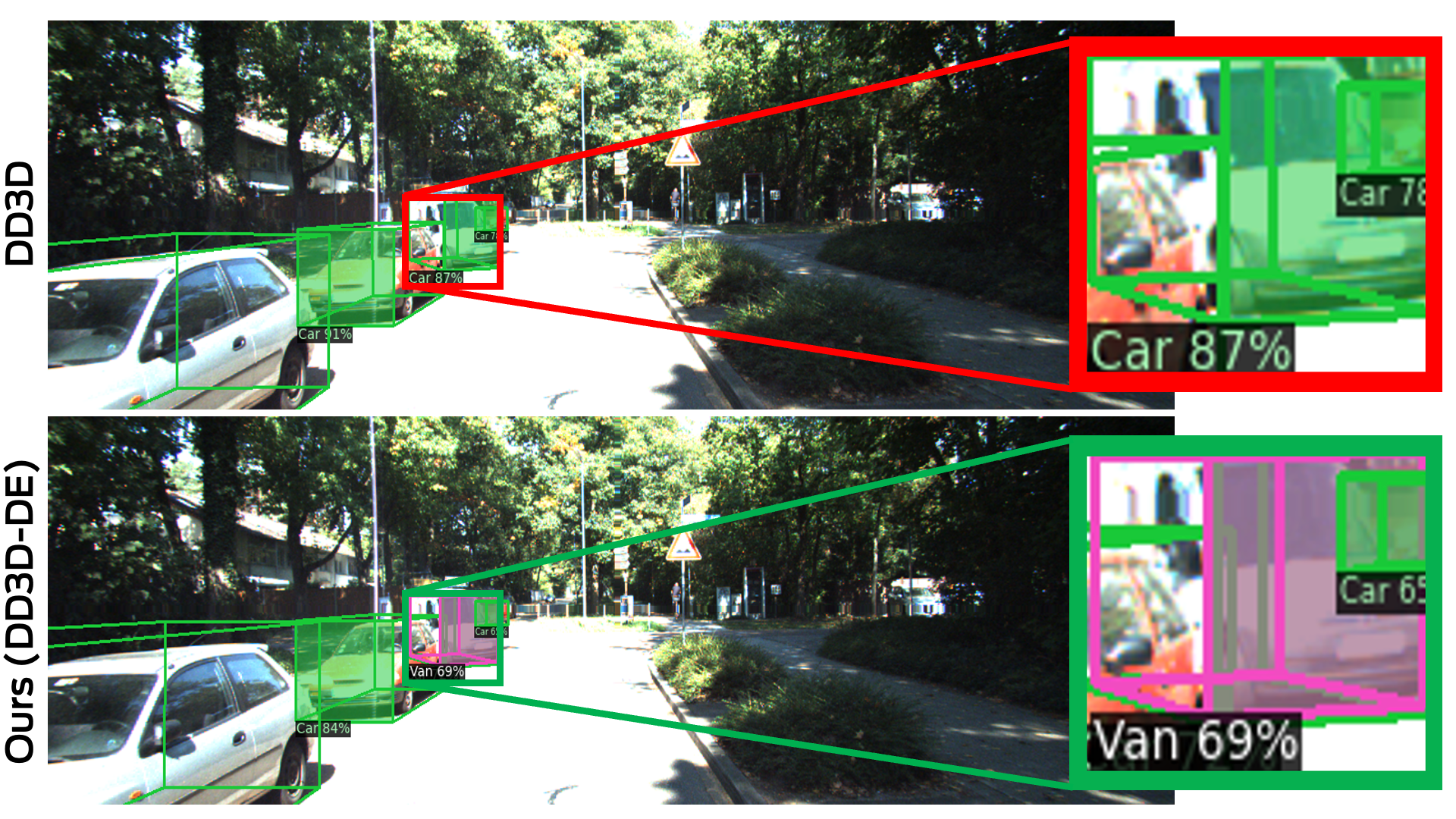
(a)

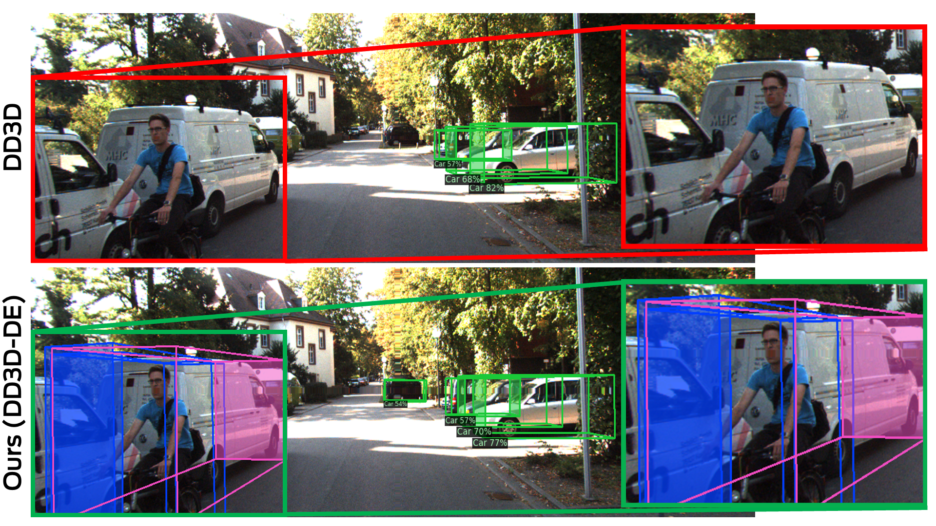
(b)

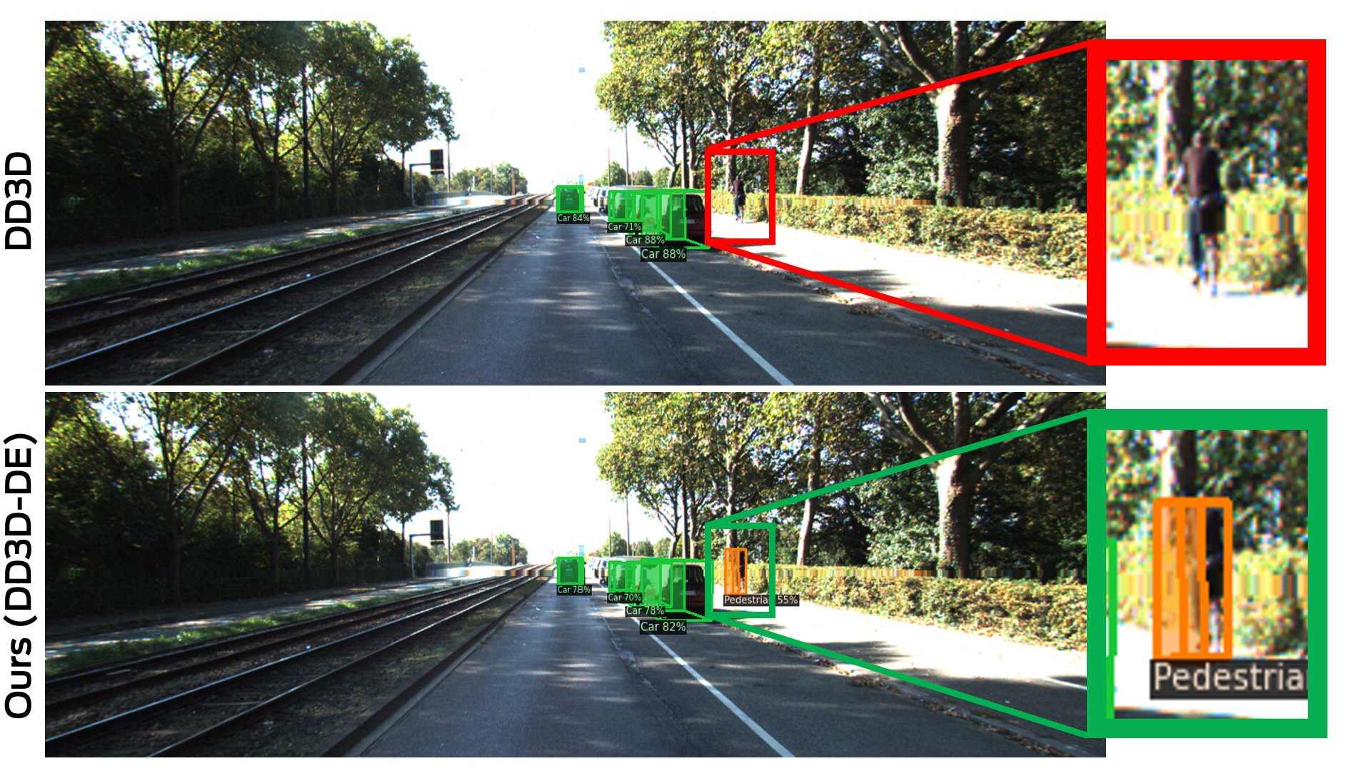
(c)

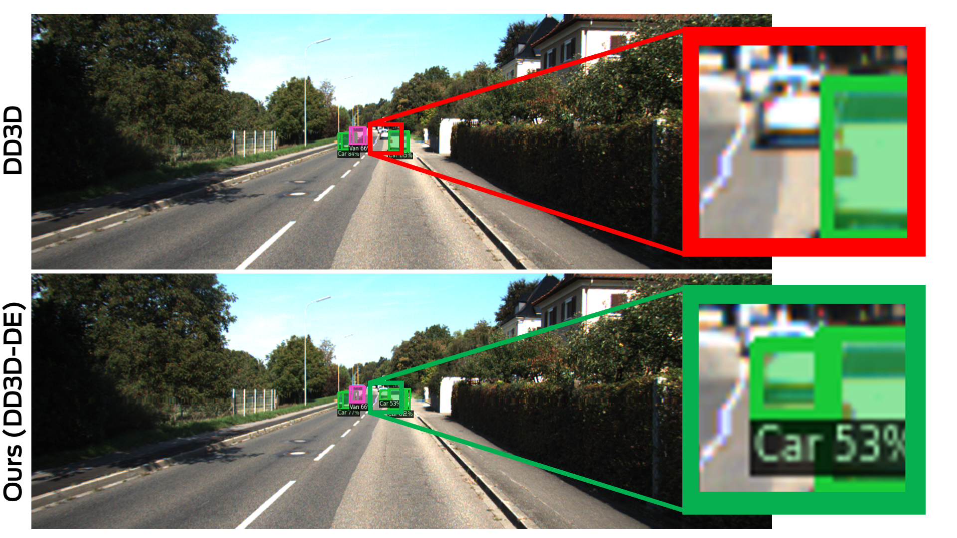
(d)

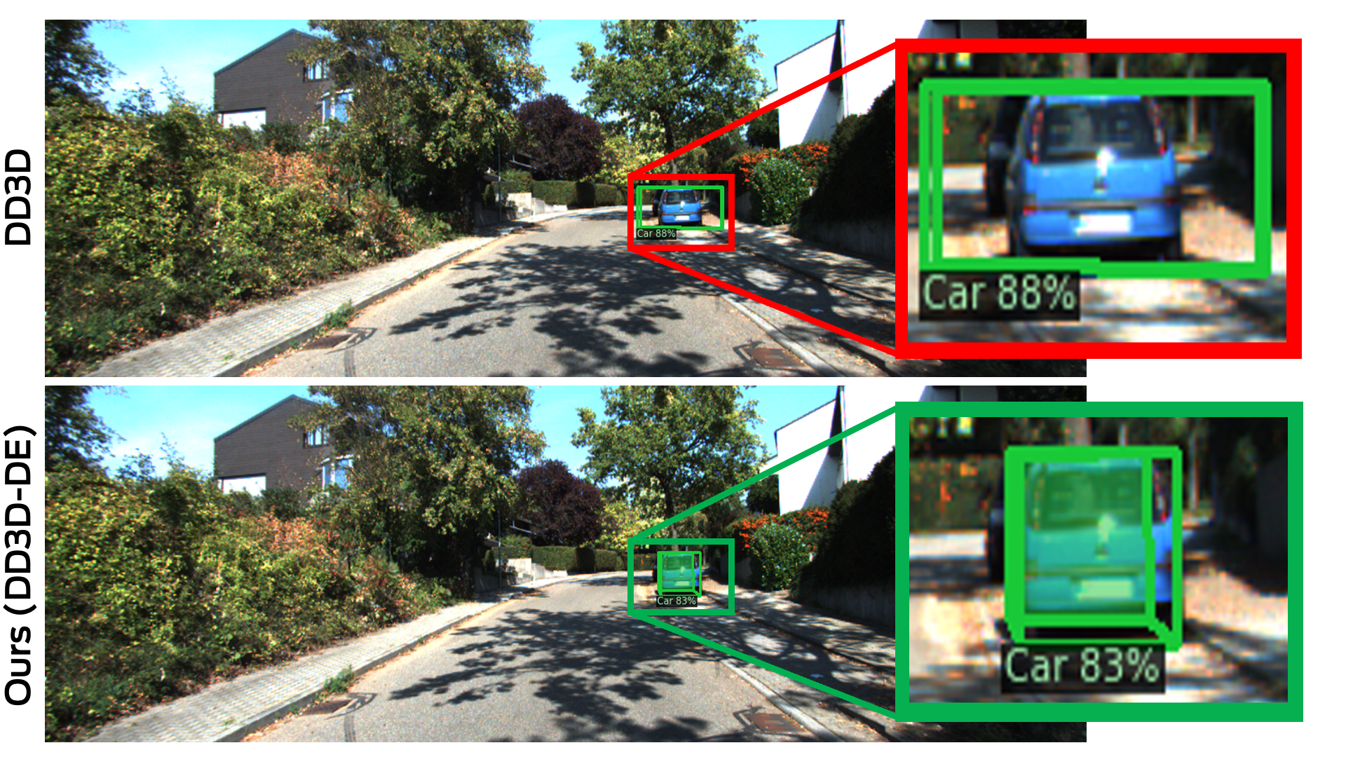
(e)

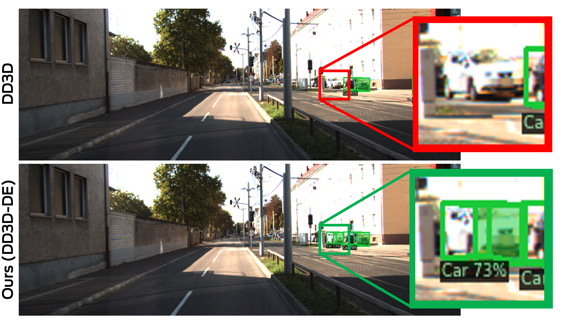
(f)

Figure 6: Qualitative analysis of predictions from the baseline DD3D model and our DD3D-DE model. The samples shown here were randomly drawn from the split of the KITTI test split. As shown in the images, DD3D-DE improves the performance over the baseline model on under-represented, and out-of-distribution samples containing objects such as Van, Cyclist, and occluded or far away Car

.

BEVFormer: Experiments with BEVFormer was done on with two different variants of the network architectures: (1) BEVFormer-base, and (2) BEVFormer-small. Both architectures used ResNet-101 [17] as the backbone network. With the official codebase , we were unable to reproduce the results reported in the paper, and hence, the baseline metrics reported in this paper were computed by retraining the models from scratch. These results are summarized in Tables 4 and 5.

Table 4: 3D detection results with DD3D on nuScenes test set. The suffix DE signifies our method of applying Generalized Focal Loss weights to each sample. R101 in the table is refers to the ResNet-101 backbone. Best NDS and mAP scores are highlighted in bold.

Method	Backbone	$\eta$	$\gamma$	NDS$\uparrow$	$\Delta$	mAP$\uparrow$	$\Delta$	mATE$\downarrow$	mASE$\downarrow$	mAOE$\downarrow$	mAVE$\downarrow$	mAAE$\downarrow$
FCOS3D [46]	R101	-	-	0.428	-	0.358	-	0.690	0.249	0.452	1.434	0.124
PGD [47]	R101	-	-	0.448	-	0.386	-	0.626	0.245	0.451	1.509	0.127
BEVFormer-base	R101	-	-	0.5196	-	0.4242	-	0.6351	0.2684	0.4219	0.4593	0.1406
BEVFormer-base-DE	R101	3.0	5.0	0.5198	(0.04%)	0.4303	(1.44%)	0.6369	0.2706	0.4418	0.4649	0.1388

Table 5: 3D detection results with BEVFormer on nuScenes val set. BEVFormer-sml stands for the BEVFormer-small variant, and the suffix DE signifies our method of applying Generalized Focal Loss weights to each sample. R101 in the table is refers to the ResNet-101 backbone. Best NDS and mAP scores are highlighted in bold.

Method	Backbone	$\eta$	$\gamma$	NDS$\uparrow$	$\Delta$	mAP$\uparrow$	$\Delta$	mATE$\downarrow$	mASE$\downarrow$	mAOE$\downarrow$	mAVE$\downarrow$	mAAE$\downarrow$
BEVFormer-sml	R101	-	-	0.3874	-	0.3516	-	0.787	0.2885	0.4981	1.169	0.3101
BEVFormer-sml-DE	R101	0.5	2.0	0.3907	(0.85%)	0.3544	(0.80%)	0.7687	0.2904	0.4952	1.174	0.3104
BEVFormer-sml-DE	R101	1.0	2.0	0.39	(0.67%)	0.3552	(1.02%)	0.7774	0.2925	0.4965	1.148	0.3094
FCOS3D [46]	R101	-	-	0.415	-	0.343	-	0.725	0.263	0.422	1.292	0.153
PGD [47]	R101	-	-	0.428	-	0.369	-	0.683	0.260	0.439	1.268	0.185
DETR3D [48]	R101	-	-	0.425	-	0.346	-	0.773	0.268	0.383	0.842	0.216
BEVFormer-base	R101	-	-	0.5056	-	0.4071	-	0.6843	0.278	0.3953	0.4241	0.1973
BEVFormer-base-DE	R101	3.0	5.0	0.5069	(0.26%)	0.4084	(0.32%)	0.6854	0.2775	0.3911	0.4225	0.1969

Table 6: 3D detection results with BEVFusion on nuScenes val set. BevFusion-C stands for the BevFusion-Camera only variant, BevFusion-C-NS stands for BevFusion-Camera Only No class balanced sampling. The suffix DE signifies our method of applying Generalized Focal Loss weights to each sample. SwinT in the table is refers to the Swin Transformer backbone. Best NDS and mAP scores are highlighted in bold.

Method	Backbone	$\eta$	$\gamma$	NDS $\uparrow$	$\Delta$	mAP $\uparrow$	$\Delta$	mATE$\downarrow$	mASE$\downarrow$	mAOE$\downarrow$	mAVE$\downarrow$	mAAE$\downarrow$
BEVFusion-C	Swin-T	-	-	0.3954	-	0.3253	-	0.6992	0.2778	0.6135	0.8205	0.2612
BEVFusion-C-DE	Swin-T	0.3	5.0	0.4008	(1.36%)	0.3287	(1.05%)	0.6709	0.2691	0.5958	0.8440	0.2558
BEVFusion-C-NC	Swin-T	-	-	0.3382	-	0.3196	-	0.7630	0.2791	0.7762	1.2526	0.3970
BEVFusion-C-NC-DE	Swin-T	0.3	5.0	0.3741	(10.61%)	0.3114	(-2.56%)	0.7760	0.2699	0.5314	0.9467	0.2918

BEVFusion camera only model has been trained from scratch as the baseline model, which uses Swin Transformer pretrained on nuImages as the backbone network. With the official code-base , we have been able to obtain similar baseline results ($0.3954$ NDS), and further improve them with Generalized Focal Loss. Detailed results are in Table 6.

For all experiments with BEVFormer, $16$ NVIDIA A100 GPUs were used, and the models were trained with a learning rate of $2\times 10^{-4}$ along with CosineAnnealing scheduler for a total of $24$ epochs. For BEVFusion, all experiments used 8 NVIDIA A100 GPUS trained for 20 epochs.

Dataset Bias Quantification: For Waymo Dataset Analysis, our experiments have been conducted on the front camera subset($200,000$) of the Waymo training set split(1 million images). Using resnet101 for feature extraction, followed by TSNE and DBSCAN to compute clusters for lower dimensional space. As indicated in Fig.2-(d), with the visualization on most likely clusters of dataset samples, several semantically meaningful clusters have formed, namely cluster $92$ of city crosswalk, cluster $62$ of the residential driving scene of palm trees, cluster $39$ of crowded driving scenes, and cluster 32 of construction vehicles and traffic cones. Similarly, the BDD100K dataset contains mostly two scenarios - daylight and nighttime( Fig.2 -(c) ).

5 Further Discussion

It is worth noting that the proposed generalized focal loss function has been tested end-to-end on two autonomous driving datasets and in the context of 3D object detection. Semantics-based dataset distribution has been analyzed and bias has been quantified for $2$ additional datasets, and the results demonstrate that those datasets could also benefit from our loss function. It is possible that this loss function may also be effective for other tasks, but this has not yet been explored. Parameters used in this paper for t-SNE and DBSCAN were chosen analytically by visualizing the cluster and samples from each of them.

6 Conclusion

While prior work tackles explicit class imbalance, this paper addresses the overlooked issue of implicit dataset bias caused by non-uniform sample likelihoods. By modeling raw image data instead of just categorical labels, the proposed likelihood computation and Generalized Focal Loss reweight training in a ground-truth agnostic manner. Experiments demonstrate improved rare and out-of-distribution sample modeling over state-of-the-art techniques relying solely on class frequencies. The consistent gains highlight the benefits of understanding dataset heterogeneity beyond class labels alone. This likelihood-based approach provides a useful complement to existing class-aware balancing methods. By countering biases in the raw visual distribution itself, it opens promising new directions for unsupervised analysis and optimization. The principles explored in this work can enable future research on minimizing implicit dataset imbalances.

Supplementary Materials
DatasetEquity: Are All Samples Created Equal?
In The Quest For Equity Within Datasets

Appendix A Dataset cluster visualization

Camera images from various datasets are first passed through a feature extractor, followed by a low-dimensional feature projection (t-SNE). These low-dimensional (3D) features are then clustered together to reveal frames with similar semantics and perceptual details. The relative size of each of these clusters is then used as a proxy for quantifying the likelihood of occurrence for each sample within those clusters. Figure S1 visualizes these clusters in 2D for the four datasets analyzed in this work.

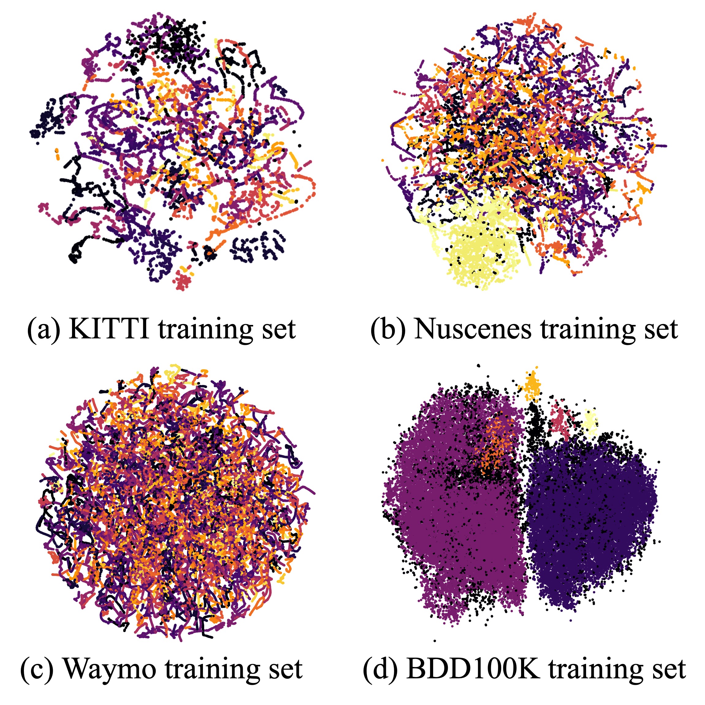
Figure S1: NuScenes, KITTI, Waymo, and BDD100k dataset samples projected onto a 3-dimensional t-SNE space and then clustered using DBSCAN (only first 2-dimensions are visualized). Each color represents a unique cluster ID. Only a single front camera image was used to compute these clusters.

Appendix B Dataset samples visualization

A few examples of samples from various clusters and their scaled likelihoods are shown in sections B.1, C, D, and E. These clusters were computed by first projecting $2048$-dimensional image embeddings onto a lower $3$-dimensional space using t-SNE, and then applying the DBSCAN algorithm. The likelihood of each sample is then computed as $\mathcal{L}_{s^{(i)}}=\frac{|C_{i}|}{\max_{i}(|C_{i}|)}$, where $C_{i}$ refers to the $i^{th}$ cluster, $|C_{i}|$ is the number of samples in the $i^{th}$ cluster, and $\mathcal{L}_{s^{(i)}}$ is the scaled likelihood of samples corresponding to the $i^{th}$ cluster. Corresponding to each row in the visualized samples below, we also provide the measure for corresponding likelihood values. All images in a certain row are taken from the same cluster.

B.1 KITTI training dataset

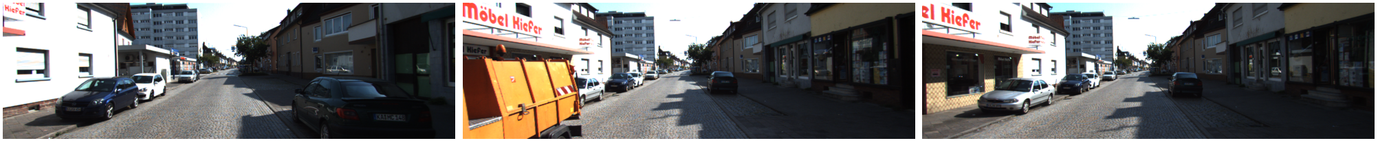
(a)

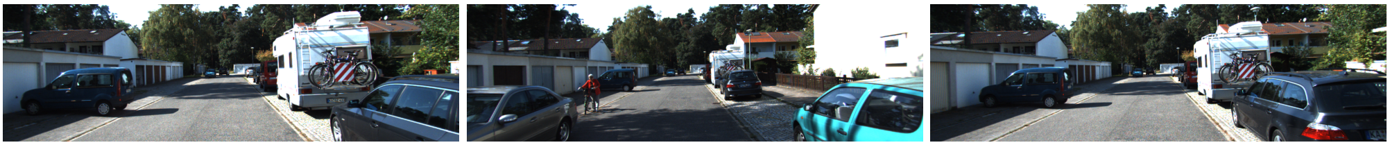
(b)

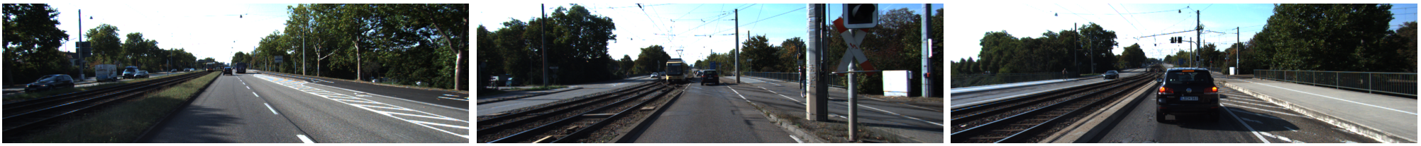
(c)

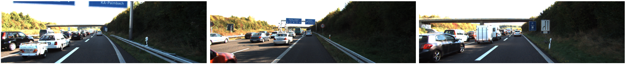
(d)

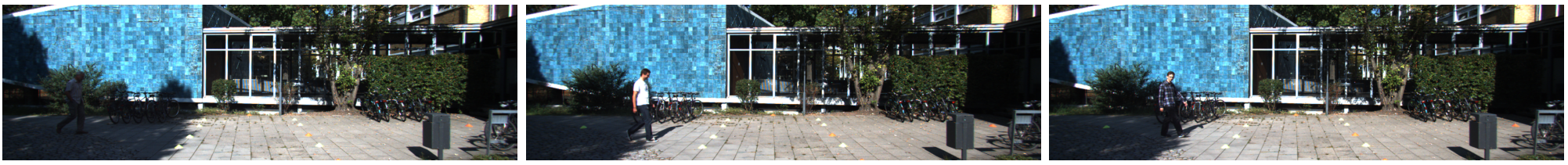
(e)

Figure S2: Samples from various clusters in KITTI training dataset, and their likelihoods relative to the largest cluster within the dataset. Samples shown in the last row come from a cluster of size $416$, and is the largest among all clusters.

Appendix C nuScenes training dataset

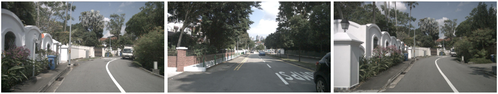
(a)

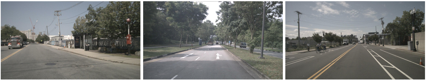
(b)

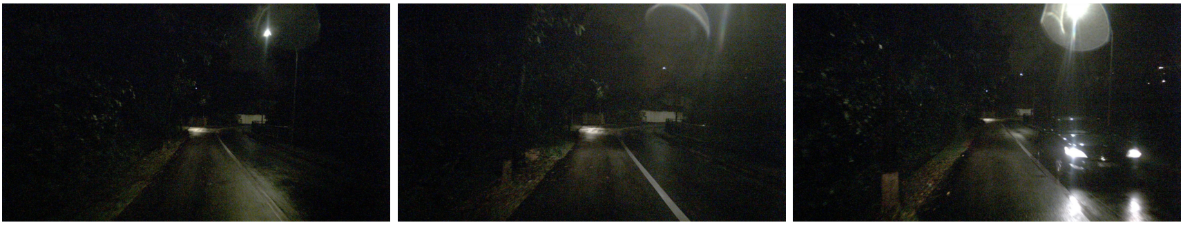
(c)

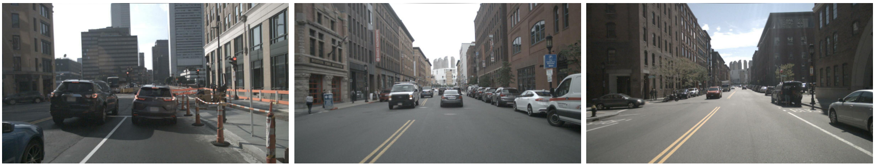
(d)

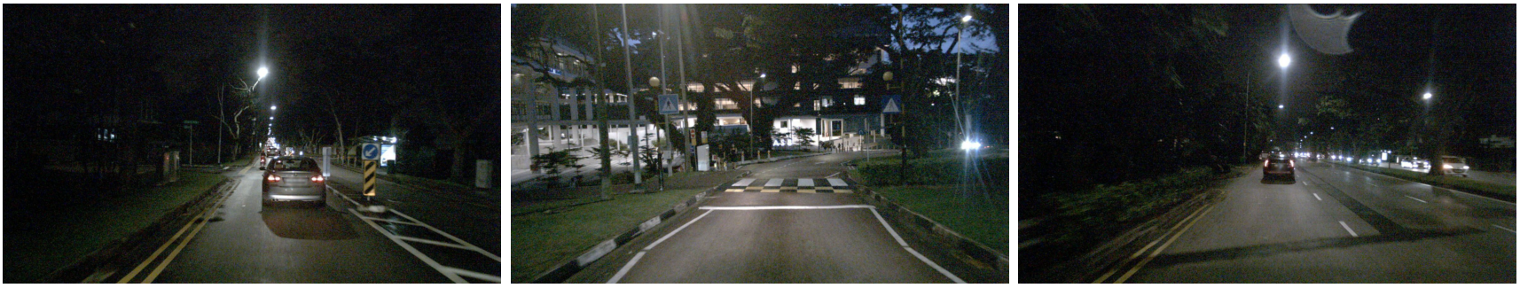
(e)

Figure S3: Samples from various clusters in nuScenes training dataset, and their likelihoods relative to the largest cluster within the dataset. Samples shown in the last row come from a cluster of size $2344$, and is the largest among all clusters.

Appendix D Waymo Open dataset

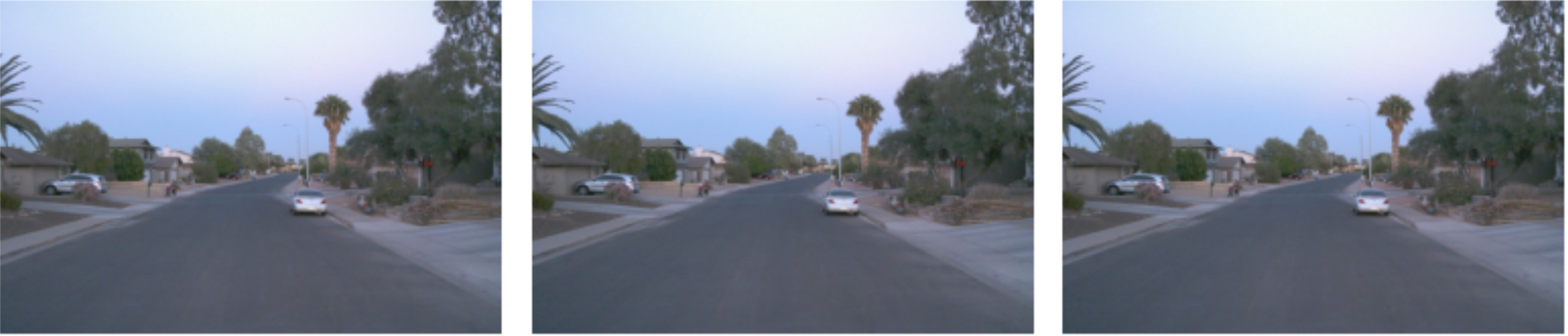
(a)

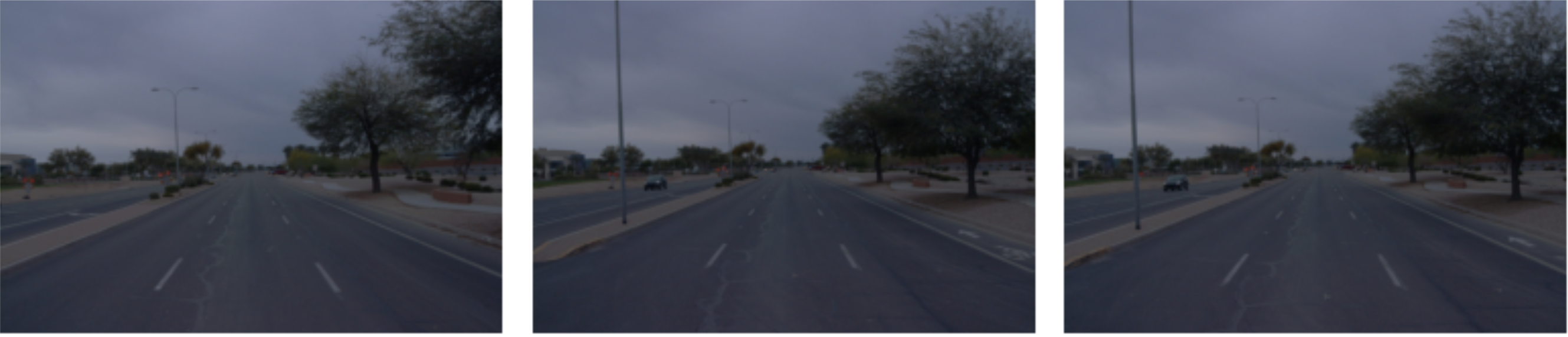
(b)

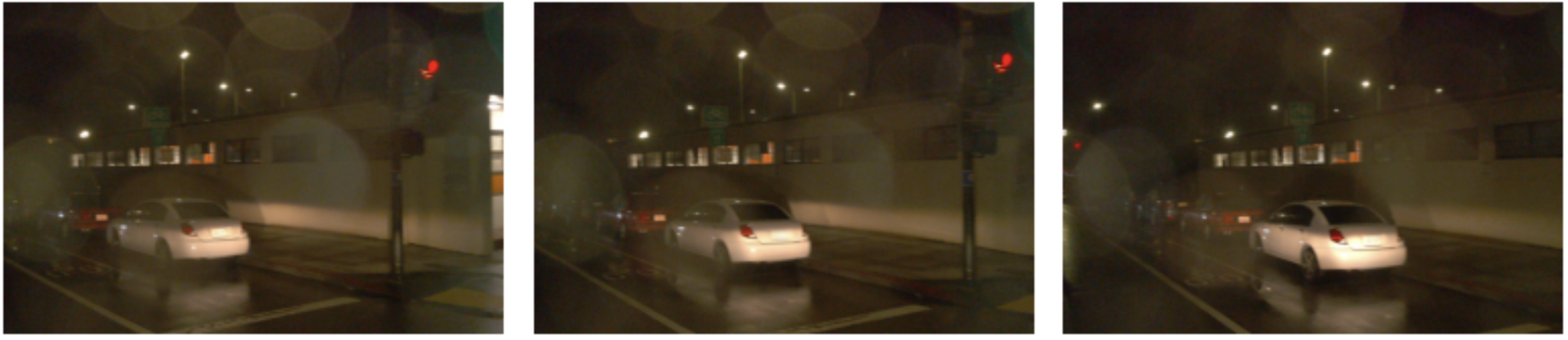
(c)

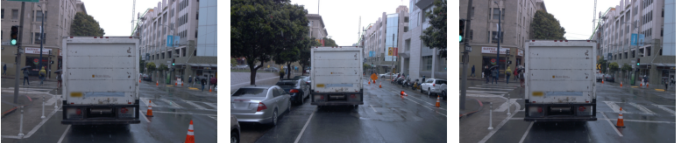
(d)

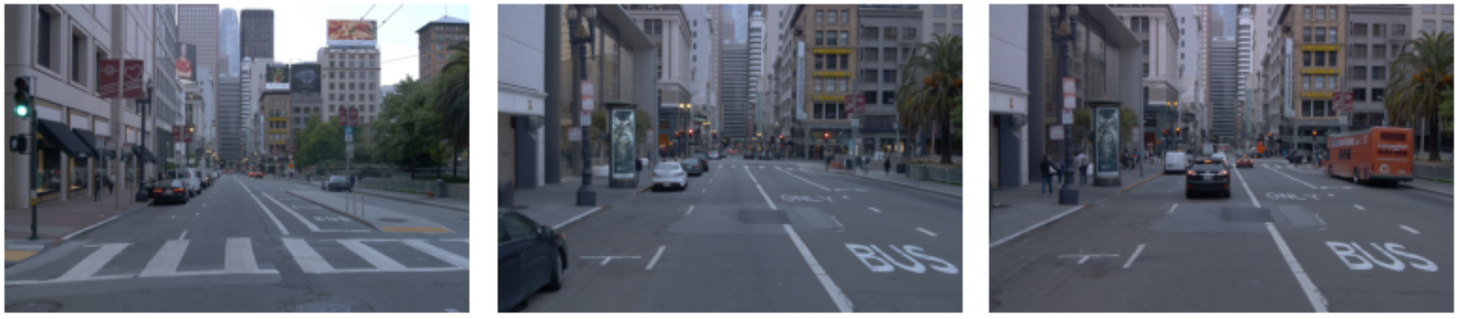
(e)

Figure S4: Samples from various clusters in Waymo training dataset, and their likelihoods relative to the largest cluster within the dataset. Totally, $1408$ clusters formed within the $200000$ training samples from the front camera. The rarest clusters contain (a) (b) and (c) of only 10 samples each in the empty residential driving scene, after-sunset scene, and high rainy scene respectively. Samples shown in the last row come from cluster $87$ of size $796$, and is the largest among all clusters. The rest top largest clusters share similar cluster sizes of $500$ to $700$ samples from urban city driving scenes, which indicates the Waymo training set is very well balanced.

Appendix E BDD100K training dataset

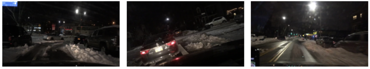
(a)

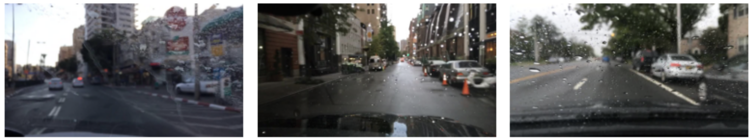
(b)

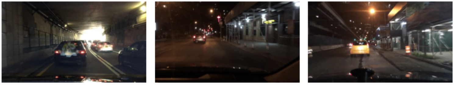
(c)

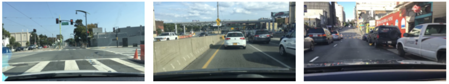
(d)

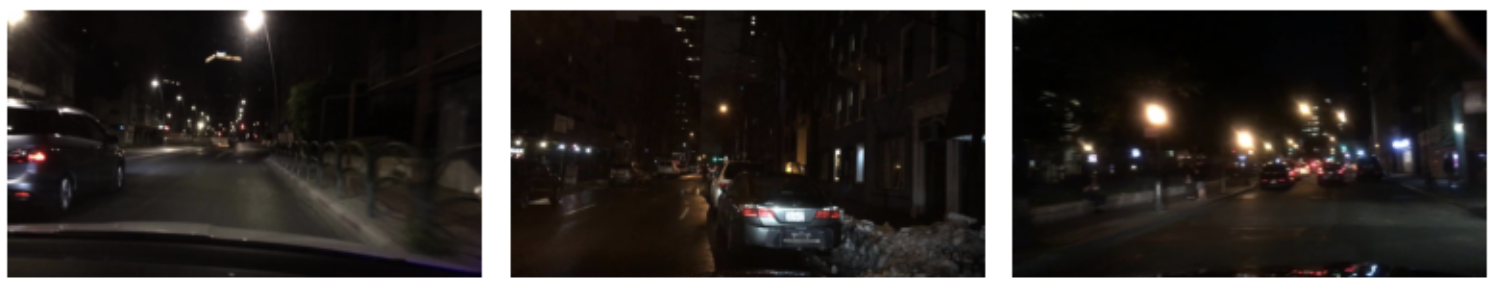
(e)

Figure S5: Samples from various clusters in BDD100K training dataset, and their likelihoods relative to the largest cluster within the dataset. Samples shown in the last row come from a cluster of size $23385$, and is the largest among all clusters. The smallest cluster shown in the top row contains only $116$ samples.

References

- [1] Björn Barz and Joachim Denzler. Hierarchy-based image embeddings for semantic image retrieval. In 2019 IEEE Winter Conference on Applications of Computer Vision (WACV), pages 638–647, 2019.
- [2] Paula Branco, Luís Torgo, and Rita P. Ribeiro. A survey of predictive modeling on imbalanced domains. ACM Comput. Surv., 49(2), aug 2016.
- [3] Garrick Brazil and Xiaoming Liu. M3d-rpn: Monocular 3d region proposal network for object detection. In Proceedings of the IEEE International Conference on Computer Vision, Seoul, South Korea, 2019.
- [4] Jonathon Byrd and Zachary C. Lipton. Weighted risk minimization & deep learning. CoRR, abs/1812.03372, 2018.
- [5] Holger Caesar, Varun Bankiti, Alex H. Lang, Sourabh Vora, Venice Erin Liong, Qiang Xu, Anush Krishnan, Yu Pan, Giancarlo Baldan, and Oscar Beijbom. nuscenes: A multimodal dataset for autonomous driving. In CVPR, 2020.
- [6] Ricardo JGB Campello, Davoud Moulavi, and Jörg Sander. Density-based clustering based on hierarchical density estimates. In Advances in Knowledge Discovery and Data Mining: 17th Pacific-Asia Conference, PAKDD 2013, Gold Coast, Australia, April 14-17, 2013, Proceedings, Part II 17, pages 160–172. Springer, 2013.
- [7] Mathilde Caron, Hugo Touvron, Ishan Misra, Hervé Jégou, Julien Mairal, Piotr Bojanowski, and Armand Joulin. Emerging properties in self-supervised vision transformers. In Proceedings of the International Conference on Computer Vision (ICCV), 2021.
- [8] Xiaozhi Chen, Kaustav Kundu, Yukun Zhu, Andrew G Berneshawi, Huimin Ma, Sanja Fidler, and Raquel Urtasun. 3d object proposals for accurate object class detection. In C. Cortes, N. Lawrence, D. Lee, M. Sugiyama, and R. Garnett, editors, Advances in Neural Information Processing Systems, volume 28. Curran Associates, Inc., 2015.
- [9] Yin Cui, Menglin Jia, Tsung-Yi Lin, Yang Song, and Serge Belongie. Class-balanced loss based on effective number of samples. In CVPR, 2019.
- [10] Martin Ester, Hans-Peter Kriegel, Jörg Sander, and Xiaowei Xu. A density-based algorithm for discovering clusters in large spatial databases with noise. In Proceedings of the Second International Conference on Knowledge Discovery and Data Mining, KDD’96, page 226–231. AAAI Press, 1996.
- [11] Pedro F. Felzenszwalb, Ross B. Girshick, and David McAllester. Cascade object detection with deformable part models. In 2010 IEEE Computer Society Conference on Computer Vision and Pattern Recognition, pages 2241–2248, 2010.
- [12] K. Ruwani M. Fernando and Chris P. Tsokos. Dynamically weighted balanced loss: Class imbalanced learning and confidence calibration of deep neural networks. IEEE Transactions on Neural Networks and Learning Systems, 33(7):2940–2951, 2022.
- [13] Siddhartha Gairola, Rajvi Shah, and P.J. Narayanan. Unsupervised image style embeddings for retrieval and recognition tasks. In 2020 IEEE Winter Conference on Applications of Computer Vision (WACV), pages 3270–3278, 2020.
- [14] Andreas Geiger, Philip Lenz, and Raquel Urtasun. Are we ready for autonomous driving? the kitti vision benchmark suite. In Conference on Computer Vision and Pattern Recognition (CVPR), 2012.
- [15] Haibo He and Edwardo A. Garcia. Learning from imbalanced data. IEEE Transactions on Knowledge and Data Engineering, 21(9):1263–1284, 2009.
- [16] Kaiming He, Xiangyu Zhang, Shaoqing Ren, and Jian Sun. Deep residual learning for image recognition. CoRR, abs/1512.03385, 2015.
- [17] Kaiming He, Xiangyu Zhang, Shaoqing Ren, and Jian Sun. Deep residual learning for image recognition. In 2016 IEEE Conference on Computer Vision and Pattern Recognition (CVPR), pages 770–778, 2016.
- [18] Junjie Huang, Guan Huang, Zheng Zhu, Ye Yun, and Dalong Du. Bevdet: High-performance multi-camera 3d object detection in bird-eye-view. arXiv preprint arXiv:2112.11790, 2021.
- [19] Nikita Jaipuria, Katherine Stevo, Xianling Zhang, Meghana L. Gaopande, Ian Calle Garcia, Jinesh Jain, and Vidya N. Murali. deeppic: Deep perceptual image clustering for identifying bias in vision datasets. In 2022 IEEE/CVF Conference on Computer Vision and Pattern Recognition Workshops (CVPRW), pages 4792–4801, 2022.
- [20] Nikita Jaipuria, Xianling Zhang, Rohan Bhasin, Mayar Arafa, Punarjay Chakravarty, Shubham Shrivastava, Sagar Manglani, and Vidya N. Murali. Deflating dataset bias using synthetic data augmentation. In Proceedings of the IEEE/CVF Conference on Computer Vision and Pattern Recognition (CVPR) Workshops, June 2020.
- [21] I.T. Jolliffe. Principal Component Analysis. Springer Verlag, 1986.
- [22] Akshay Krishnan, Amit Raj, Xianling Zhang, Alexandra Carlson, Nathan Tseng, Sandhya Sridhar, Nikita Jaipuria, and James Hays. Lane: Lighting-aware neural fields for compositional scene synthesis, 2023.
- [23] Youngwan Lee and Jongyoul Park. Centermask: Real-time anchor-free instance segmentation. 2020.
- [24] Yingwei Li, Adams Wei Yu, Tianjian Meng, Ben Caine, Jiquan Ngiam, Daiyi Peng, Junyang Shen, Yifeng Lu, Denny Zhou, Quoc V Le, et al. Deepfusion: Lidar-camera deep fusion for multi-modal 3d object detection. In Proceedings of the IEEE/CVF Conference on Computer Vision and Pattern Recognition, pages 17182–17191, 2022.
- [25] Zhiqi Li, Wenhai Wang, Hongyang Li, Enze Xie, Chonghao Sima, Tong Lu, Qiao Yu, and Jifeng Dai. Bevformer: Learning bird’s-eye-view representation from multi-camera images via spatiotemporal transformers, 2022.
- [26] Tsung-Yi Lin, Priya Goyal, Ross B. Girshick, Kaiming He, and Piotr Dollár. Focal loss for dense object detection. CoRR, abs/1708.02002, 2017.
- [27] George C Linderman and Stefan Steinerberger. Clustering with t-sne, provably. SIAM Journal on Mathematics of Data Science, 1(2):313–332, 2019.
- [28] Zhijian Liu, Haotian Tang, Alexander Amini, Xingyu Yang, Huizi Mao, Daniela Rus, and Song Han. Bevfusion: Multi-task multi-sensor fusion with unified bird’s-eye view representation. arXiv, 2022.
- [29] Leland McInnes, John Healy, and Steve Astels. hdbscan: Hierarchical density based clustering. Journal of Open Source Software, 2(11):205, 2017.
- [30] Su Pang, Daniel Morris, and Hayder Radha. Clocs: Camera-lidar object candidates fusion for 3d object detection. 2020.
- [31] Dennis Park, Rares Ambrus, Vitor Guizilini, Jie Li, and Adrien Gaidon. Is pseudo-lidar needed for monocular 3d object detection? In IEEE/CVF International Conference on Computer Vision (ICCV), 2021.
- [32] Alec Radford, Jong Wook Kim, Chris Hallacy, Aditya Ramesh, Gabriel Goh, Sandhini Agarwal, Girish Sastry, Amanda Askell, Pamela Mishkin, Jack Clark, et al. Learning transferable visual models from natural language supervision. In International Conference on Machine Learning, pages 8748–8763. PMLR, 2021.
- [33] Alec Radford, Jong Wook Kim, Chris Hallacy, Aditya Ramesh, Gabriel Goh, Sandhini Agarwal, Girish Sastry, Amanda Askell, Pamela Mishkin, Jack Clark, Gretchen Krueger, and Ilya Sutskever. Learning transferable visual models from natural language supervision. CoRR, abs/2103.00020, 2021.
- [34] Shaoqing Ren, Kaiming He, Ross Girshick, and Jian Sun. Faster r-cnn: Towards real-time object detection with region proposal networks. In C. Cortes, N. Lawrence, D. Lee, M. Sugiyama, and R. Garnett, editors, Advances in Neural Information Processing Systems, volume 28. Curran Associates, Inc., 2015.
- [35] Abhinav Shrivastava, Abhinav Gupta, and Ross B. Girshick. Training region-based object detectors with online hard example mining. CoRR, abs/1604.03540, 2016.
- [36] Shubham Shrivastava. Vr3dense: Voxel representation learning for 3d object detection and monocular dense depth reconstruction. arXiv preprint arXiv:2104.05932, 2021.
- [37] Shubham Shrivastava and Punarjay Chakravarty. Cubifae-3d: Monocular camera space cubification for auto-encoder based 3d object detection, 2020.
- [38] Andrea Simonelli, Samuel Rota Bulo, Lorenzo Porzi, Manuel López-Antequera, and Peter Kontschieder. Disentangling monocular 3d object detection. In Proceedings of the IEEE/CVF International Conference on Computer Vision, pages 1991–1999, 2019.
- [39] Andrea Simonelli, Samuel Rota Bulò, Lorenzo Porzi, Manuel López-Antequera, and Peter Kontschieder. Disentangling monocular 3d object detection. 2019 IEEE/CVF International Conference on Computer Vision (ICCV), pages 1991–1999, 2019.
- [40] Andrea Simonelli, Samuel Rota Bulò, Lorenzo Porzi, Manuel López Antequera, and Peter Kontschieder. Disentangling monocular 3d object detection: From single to multi-class recognition. IEEE Transactions on Pattern Analysis and Machine Intelligence, 44(3):1219–1231, 2022.
- [41] Pei Sun, Henrik Kretzschmar, Xerxes Dotiwalla, Aurelien Chouard, Vijaysai Patnaik, Paul Tsui, James Guo, Yin Zhou, Yuning Chai, Benjamin Caine, Vijay Vasudevan, Wei Han, Jiquan Ngiam, Hang Zhao, Aleksei Timofeev, Scott Ettinger, Maxim Krivokon, Amy Gao, Aditya Joshi, Yu Zhang, Jonathon Shlens, Zhifeng Chen, and Dragomir Anguelov. Scalability in perception for autonomous driving: Waymo open dataset. In Proceedings of the IEEE/CVF Conference on Computer Vision and Pattern Recognition (CVPR), June 2020.
- [42] Kah Kay Sung and Tomaso A. Poggio. Learning and Example Selection for Object and Pattern Detection. PhD thesis, USA, 1996. AAI0800657.
- [43] Laurens van der Maaten and Geoffrey Hinton. Visualizing data using t-sne. Journal of Machine Learning Research, 9(86):2579–2605, 2008.
- [44] P. Viola and M. Jones. Rapid object detection using a boosted cascade of simple features. In Proceedings of the 2001 IEEE Computer Society Conference on Computer Vision and Pattern Recognition. CVPR 2001, volume 1, pages I–I, 2001.
- [45] Lin Wang, Chaoli Wang, Zhanquan Sun, Shuqun Cheng, and Lei Guo. Class balanced loss for image classification. IEEE Access, 8:81142–81153, 2020.
- [46] Tai Wang, Xinge Zhu, Jiangmiao Pang, and Dahua Lin. Fcos3d: Fully convolutional one-stage monocular 3d object detection. In IEEE/CVF Conference on International Conference on Computer Vision Workshops, 2021.
- [47] Tai Wang, Xinge Zhu, Jiangmiao Pang, and Dahua Lin. Probabilistic and geometric depth: Detecting objects in perspective. In Conference on Robot Learning, 2021.
- [48] Yue Wang, Vitor Campagnolo Guizilini, Tianyuan Zhang, Yilun Wang, Hang Zhao, and Justin Solomon. DETR3d: 3d object detection from multi-view images via 3d-to-2d queries. In 5th Annual Conference on Robot Learning, 2021.
- [49] Fisher Yu, Haofeng Chen, Xin Wang, Wenqi Xian, Yingying Chen, Fangchen Liu, Vashisht Madhavan, and Trevor Darrell. Bdd100k: A diverse driving dataset for heterogeneous multitask learning. In Proceedings of the IEEE/CVF conference on computer vision and pattern recognition, pages 2636–2645, 2020.
- [50] Xianling Zhang, Nathan Tseng, Ameerah Syed, Rohan Bhasin, and Nikita Jaipuria. Simbar: Single image-based scene relighting for effective data augmentation for automated driving vision tasks. In Proceedings of the IEEE/CVF Conference on Computer Vision and Pattern Recognition (CVPR), pages 3718–3728, June 2022.
- [51] Yunpeng Zhang, Zheng Zhu, Wenzhao Zheng, Junjie Huang, Guan Huang, Jie Zhou, and Jiwen Lu. Beverse: Unified perception and prediction in birds-eye-view for vision-centric autonomous driving. arXiv preprint arXiv:2205.09743, 2022.
- [52] Benjin Zhu, Zhengkai Jiang, Xiangxin Zhou, Zeming Li, and Gang Yu. Class-balanced grouping and sampling for point cloud 3d object detection, 2019.