Tensor-Compressed Back-Propagation-Free Training for
(Physics-Informed) Neural Networks

Abstract

Backward propagation (BP) is widely used to compute the gradients in neural network training. However, it is hard to implement BP on edge devices due to the lack of hardware and software resources to support automatic differentiation. This has tremendously increased the design complexity and time-to-market of on-device training accelerators. This paper presents a completely BP-free framework that only requires forward propagation to train realistic neural networks. Our technical contributions are three-fold. Firstly, we present a tensor-compressed variance reduction approach to greatly improve the scalability of zeroth-order (ZO) optimization, making it feasible to handle a network size that is beyond the capability of previous ZO approaches. Secondly, we present a hybrid gradient evaluation approach to improve the efficiency of ZO training. Finally, we extend our BP-free training framework to physics-informed neural networks (PINNs) by proposing a sparse-grid approach to estimate the derivatives in the loss function without using BP. Our BP-free training only loses little accuracy on the MNIST dataset compared with standard first-order training. We also demonstrate successful results in training a PINN for solving a 20-dim Hamiltonian-Jacobi-Bellman PDE. This memory-efficient and BP-free approach may serve as a foundation for the near-future on-device training on many resource-constraint platforms (e.g., FPGA, ASIC, micro-controllers, and photonic chips).

1 Introduction

In neural network training, it is widely assumed that the gradient information can be computed via backward propagation (BP) (Rumelhart, Hinton, and Williams 1986) to perform SGD-type optimization. This is true on HPC and desktop computers, because they support Pytorch/Tensorflow backend and automatic differentiation (AD) packages (Bolte and Pauwels 2020) to compute exact gradients. However, performing BP is infeasible on many edge devices (e.g., FPGA, ASIC, photonic chips, embedded micro-processors) due to the lack of necessary computing and memory resources to support AD libraries. Manually calculating the gradient of a modern neural network on edge hardware is time-consuming due to the high complexity and lots of debug iterations. This can significantly delay the development and deployment of AI training accelerators. For instance, designing an FPGA inference accelerator may be done within one week via high-level synthesis by an experienced AI hardware expert, but designing an FPGA training accelerator can take one or two years due to the high complexity of implementing BP. Some analog edge computing platforms (e.g., photonic chips) even do not have scalable memory arrays to store the final or intermediate results of a chain rule-based gradient computation.

This paper investigates the end-to-end training of neural networks and physics-informed neural networks (PINNs) without using BP, which can potentially make on-device neural network training accelerator design as easy as designing an inference accelerator. The demand for edge-device training has been growing rapidly in recent years. One motivation is to ensure AI model performance under varying data stream and environment, as well as device parameter shift. Another motivation is the increasing concerns about data privacy, which requires end-to-end or incremental learning on edge devices based on local data (McMahan et al. 2017). In science and engineering, PINNs (Raissi, Perdikaris, and Karniadakis 2019; Lagaris, Likas, and Fotiadis 1998) have been increasingly used to solve the forward and inverse problems of high-dimensional partial differential equations (PDE). A PINN needs to be trained again once the PDE initial conditions, boundary conditions, or measurement data changes. Applications of such on-device PINN training include (but are not limited to) safety-aware verification and control of autonomous systems (Bansal and Tomlin 2021; Onken et al. 2021; Sun, Jha, and Fan 2020) and MRI-based electrical property tomography (Yu et al. 2023).

We intend to perform BP-free training via stochastic zeroth-order (ZO) optimization  (Duchi et al. 2015; Nesterov and Spokoiny 2017; Ghadimi and Lan 2013; Shamir 2017; Balasubramanian and Ghadimi 2022; Liu et al. 2020a), which uses a few forward evaluations with perturbed model parameters to approximate the true gradient. In the realm of deep learning, ZO optimization was primarily used for crafting black-box adversarial examples to assess neural network robustness (Chen et al. 2017; Liu et al. 2020b), and for parameter and memory-efficient model fine-tuning (Malladi et al. 2023; Zhang et al. 2022). Notably, ZO optimization has been rarely used in neural network training from scratch, because the variance of the ZO gradient estimation is large when the number of training variables increases.

Leveraging ZO optimization, we present a scalable BP-free approach for training both standard neural networks and PINNs from scratch. Our novel contributions include:

• A hybrid and tensor-compressed ZO training approach. We first reduce the gradient variance of ZO optimization significantly via a tensor-compressed dimension reduction in the training process. This variance reduction approach enables training realistic neural networks and PINNs which are beyond the capability of existing ZO training. Then we design a hybrid approach that combines the advantages of random ZO gradient estimation and finite-difference methods to reduce the number of forward evaluations in ZO training.

• A completely BP-free approach for training PINNs. The loss function of PINNs often involves differential operators, which complicates the loss evaluation and the training process on resource-constraint edge devices. To avoid using BP in the loss evaluation, we propose a sparse-grid method to implement the Stein estimator. This allows solving vast (high-dimensional) PDE problems on edge devices where the BP computing engines are not available.

• Numerical experiments. We validate our method on the MNIST image classification task and in solving a high-dim PDE. We show that the tensor-compressed method can greatly improve the scalability of ZO training, showing better performance than sparsity-based ZO training. Our BP-free approach also shows high accuracy in solving a 20-dim Hamiltonian-Jacobi-Bellman (HJB) PDE, which is a critical task in optimal control.

While our approach still needs improvement in order to train very large neural networks (e.g., transformers), it is good enough to enable on-device training for many image, speech and scientific computing problems.

2 Background

This section introduces the necessary background of ZO optimization and PINN.

2.1 Zeroth-Order (ZO) Optimization

We consider the minimization of a loss function $\mathcal{L}(\bm{\theta})$ by updating the model parameters $\bm{\theta}\in\mathbb{R}^{d}$ iteratively using a (stochastic) gradient descent method:

$$\bm{\theta}_{t}\leftarrow\bm{\theta}_{t-1}-\alpha\bm{g}$$ (1)

where $\bm{g}$ denotes the (stochastic) gradient of the loss $\mathcal{L}$ w.r.t. model parameters $\bm{\theta}$. In some cases it is hard or even impossible to exactly compute the gradient vector $\bm{\theta}$, therefore we consider ZO optimization, which uses some forward function queries to approximate the gradient $\bm{g}$:

$$\bm{g}\approx\hat{\nabla}_{\bm{\theta}}\mathcal{L}(\bm{\theta})=\sum_{i=1}^{N}\frac{1}{N\mu}\left[\mathcal{L}\left(\bm{\theta}+\mu\bm{\xi}_{i}\right)-\mathcal{L}(\bm{\theta})\right]\bm{\xi}_{i}.$$ (2)

Here $\{\bm{\xi}_{i}\}_{i=1}^{N}$ are some perturbation vectors and $\mu$ is the sampling radius, which is typically small. Two perturbation methods are commonly used:

• Random gradient estimators (RGE): $\{\bm{\xi}_{i}\}_{i=1}^{N}$ are $N$ i.i.d. samples drawn from a distribution $\rho(\bm{\xi})$ (e.g., a multivariate Gaussian distribution).

• Coordinate-wise gradient estimator (CGE) [or finite difference (FD)]: $N=d$ and $\bm{\xi}_{i}$ denotes the i-th elementary basis vector, with one at the i-th coordinate and zeros elsewhere.

In both cases, the expectation of $\hat{\nabla}_{\bm{\theta}}\mathcal{L}$ is unbiased w.r.t. the gradient of the smoothed function $f_{\mu}(\bm{x}):=\mathbb{E}_{\bm{\xi}\sim\rho(\bm{\xi})}[f(\bm{x}+\mu\bm{\xi})]$, however biased w.r.t. the true gradient $\nabla_{\bm{\theta}}\mathcal{L}$ (Berahas et al. 2022). In comparison to CGE, RGE is typically more query-efficient, requiring a less number of function evaluations $N$ compared to the number of optimization variables $d$. The variances of both RGE and CGE involve a dimension-dependent factor $O(d/N)$ given $\mu=O(1/\sqrt{N})$ (Liu et al. 2020a).

Since the MSE error increases quickly as $d$ increases, ZO optimization was mainly used in some small- or medium-size optimization problems, such as black-box adversarial attack generation and memory-efficient fine-tuning.

2.2 Physics-Informed Neural Networks (PINNs)

Consider a generic partial differential equation (PDE):

$$\mathcal{N}[\bm{u}(\bm{x},t)] =l(\bm{x},t),~{}\quad\bm{x}\in\Omega,~{}~{}t\in[0,T],$$ (3)

$$\mathcal{I}[\bm{u}(\bm{x},0)] =g(\bm{x}),~{}~{}~{}\quad\bm{x}\in\Omega,$$

$$\mathcal{B}[\bm{u}(\bm{x},t)] =h(\bm{x},t),\quad\boldsymbol{x}\in\partial\Omega,~{}~{}t\in[0,T],$$

where $\bm{x}$ and $t$ are the spatial and temporal coordinates; $\Omega\subset\mathbb{R}^{D}$, $\partial\Omega$ and $T$ denote the spatial domain, domain boundary and time horizon, respectively; $\mathcal{N}$ is a general nonlinear differential operator; $\mathcal{I}$ and $\mathcal{B}$ represent the initial (or terminal) and boundary condition; $\bm{u}\in\mathbb{R}^{n}$ is the solution for the PDE described above. In the contexts of PINNs (Raissi, Perdikaris, and Karniadakis 2019), a solution network $\bm{u}_{\bm{\theta}}(\bm{x},t)$, parameterized by $\bm{\theta}$, is substituted into PDE (3), resulting in a residual defined as:

$$r_{\bm{\theta}}(\bm{x},t):=\mathcal{N}[\bm{u}_{\bm{\theta}}(\bm{x},t)]-l(\bm{x},t).$$ (4)

The parameters $\bm{\theta}$ can be trained by minimizing the loss:

$$\mathcal{L}(\bm{\theta})=\mathcal{L}_{r}(\bm{\theta})+\lambda_{0}\mathcal{L}_{0}(\bm{\theta})+\lambda_{b}\mathcal{L}_{b}(\bm{\theta}).$$ (5)

Here

$$\mathcal{L}_{r}(\bm{\theta}) =\frac{1}{N_{r}}\sum_{i=1}^{N_{r}}\left\|r_{\bm{\theta}}(\bm{x_{r}}^{i},t_{r}^{i})\right\|_{2}^{2},$$ (6)

$$\mathcal{L}_{0}(\bm{\theta}) =\frac{1}{N_{0}}\sum_{i=1}^{N_{0}}\left\|\mathcal{I}[\bm{u}_{\bm{\theta}}(\bm{x_{0}}^{i},0)]-g(\bm{x_{0}}^{i})\right\|_{2}^{2},$$

$$\text{and}\quad\mathcal{L}_{b}(\bm{\theta}) =\frac{1}{N_{b}}\sum_{i=1}^{N_{b}}\left\|\mathcal{B}[\bm{u}_{\bm{\theta}}(\bm{x_{b}}^{i},t_{b}^{i})]-h(\bm{x_{b}}^{i},t_{b}^{i})\right\|_{2}^{2}$$

are the residuals of the PDE, the initial (or terminal) condition and boundary condition, respectively.

3 Scaling Up ZO Optimization for Neural Network Training

This section improves the ZO method to train real-size neural networks. We first present tensor-compressed approach to dramatically reduce the gradient error and improve the scalability of ZO training. Then we present a hybrid ZO training strategy that achieves a better trade-off between accuracy and function query complexity.

3.1 Tensor-Train (TT) Variance Reduction

Our goal is to develop a BP-free training framework based on ZO optimization. As explained before, the ZO gradient estimation error is dominated by $d$, which is the number of total trainable variables. In realistic neural network training, $d$ can easily exceed $10^{5}$ even for very simple image classification problems. This prevents the direct application of ZO optimization in end-to-end neural network training.

To improve the scalability of ZO training, we propose to significantly reduce the dimensionality and gradient MSE error via a low-rank tensor-compressed training. Let $\bm{W}\in\mathbb{R}^{M\times N}$ be a generic weight matrix in a neural network. We factorize its dimension sizes as $M=\prod^{L}_{i=1}m_{i}$ and $N=\prod^{L}_{j=1}n_{j}$, fold $\bm{W}$ into a $2L$-way tensor $\mathbfcal{W}\in\mathbb{R}^{m_{1}\times m_{2}\times\dots\times m_{L}\times n_{1}\times n_{2}\times\dots\times n_{L}}$, and parameterize $\mathbfcal{W}$ with the tensor-train (TT) decomposition (Oseledets 2011):

$${\mathbfcal{W}}(i_{1},i_{2},\dots,i_{L},j_{1},j_{2},\dots,j_{L})\approx\prod^{L}\limits_{k=1}\mathbf{G}_{k}(i_{k},j_{k})$$ (7)

Here $\mathbf{G}_{k}(i_{k},j_{k})\in\mathbb{R}^{r_{k-1}\times r_{k}}$ is the $(i_{k},j_{k})$-th slice of the TT-core $\mathbfcal{G}_{k}\in\mathbb{R}^{r_{k-1}\times m_{k}\times n_{k}\times r_{k}}$by fixing its $2$nd index as $i_{k}$ and $3$rd index as $j_{k}$. The vector $(r_{0},r_{1},\dots,r_{L})$ is called TT-ranks with the constraint $r_{0}=r_{L}=1$. This TT representation reduces the number of unknown variables from $\prod^{L}\limits_{k=1}m_{k}n_{k}$ to $\sum\limits_{k=1}^{L}r_{k-1}m_{k}n_{k}r_{k}$. The compression ratio can be controlled by the TT-ranks, which can be learnt automatically via the Bayesian tensor rank determination (Hawkins and Zhang 2021; Hawkins, Liu, and Zhang 2022).

In the ZO training process, we change the training variables from $\mathbf{W}$ to the TT factors $\{\mathbfcal{G}_{k}\}_{k=1}^{L}$. This reduces the problem dimensionality $d$ by several orders of magnitude, leading to dramatic reduction of the variance in the RGE gradient estimation and of the query complexity in the CGE gradient estimator. In the ZO training, we only need forward evaluations, where the original matrix-vector product is replaced with low-cost tensor-network contraction. This offers both memory and computing cost reduction in the ZO training process. While we assume $\bm{W}$ as a weight matrix, other model parameters like embedding tables and convolution filters can be compressed simulatenously in the same way (with adjustable ranks) in the ZO training process.

3.2 A Hybrid ZO Optimizer

With the above tensor-compressed variance reduction, we can employ either RGE or CGE for ZO gradient estimation and perform BP-free training. In practice, the RGE method converges very slowly in the late stage of training due to the large gradient error. CGE needs fewer training epochs due to more accurate gradient estimation, but it needs many more forward evaluations per gradient estimation since it only perturbs one model parameter in each forward evaluation.

To enhance both the accuracy and efficiency of the whole ZO training process, we employ a hybrid ZO training scheme that involves two stages:

• ZO-signRGE coarse training: The RGE method perturbs all model parameters simultaneously with a single random perturbation, requiring significantly fewer forward queries per epoch compared to the CGE method. However, the two-level stochasticity (in SGD and in the gradient estimation, respectively) of ZO via RGE (ZO-RGE) may cause a large gradient variance and lead to divergence in high-dimensional tasks. To address this issue, we adopt the concept from signSGD (Bernstein et al. 2018) and its ZO counterpart, ZO-signSGD (Liu et al. 2019), to de-noise the ZO gradient estimation by preserving only the sign for each update:

  $$\bm{\theta}_{t}\leftarrow\bm{\theta}_{t-1}-\alpha{\rm sign}\left[\sum_{i=1}^{N}\frac{1}{N\mu}\left[\mathcal{L}\left(\bm{\theta}_{t-1}+\mu\bm{\xi}_{i}\right)-\mathcal{L}(\bm{\theta}_{t-1})\right]\bm{\xi}_{i}\right].$$

  We refer to this method as ZO-signRGE. ZO-signRGE retains only the sign of each gradient estimation, mitigating the adverse effects of the high variance of RGE. As a result, it exhibits better robustness to gradient noise and demonstrates faster empirical convergence.

• ZO-CGE fine-tuning: The CGE method requires $d+1$ forward evaluations per gradient estimation. Therefore, the ZO training with CGE (ZO-CGE) requires many function queries in the whole training process. To accelerate training, we further adopt the idea of momentum (Polyak 1964). The momentum method accumulates a velocity vector in directions of persistent reduction in the objective across iterations (Sutskever et al. 2013). The descent direction $\bm{b}^{t}$ is given by an exponential moving average of the past gradients $\bm{b}^{t}\leftarrow m\bm{b}^{t-1}+\bm{g}^{t}$. Here $m$ is the momentum term, $\bm{g}^{t}$ is the estimated gradient vector at time $t$, and $\bm{b}^{0}=\bm{g}^{0}$.

The ZO-signRGE coarse training rapidly explores a roughly converged solution with a small number of loss evaluations. When the coarse training fails to learn (e.g., the training loss exhibits trivial updates for several epochs), the optimizer switches to ZO-CGE to fine-tune the model.

4 BP-free Training for PINN

In this section, we extend the proposed TT-compressed hybrid ZO training to PINNs. Training a PINN is more challenging because the loss function in (5) involves first or even high-order derivatives. We intend to also avoid BP computation in the loss evaluation.

4.1 Stein Gradient Estimation

Without loss of generality, for an input $\bm{x}\in\mathbb{R}^{D}$ and an approximated PDE solution $\bm{u}_{\bm{\theta}}(\bm{x})\in\mathbb{R}^{n}$ parameterized by $\bm{\theta}$, we consider the first-order derivative $\nabla_{\bm{x}}\bm{u}_{\bm{\theta}}$ and Laplacian $\Delta\bm{u}_{\bm{\theta}}$ involved in the loss function of a PINN training. Our implementation leverages the Stein estimator (Stein 1981). Specifically, we represent the PDE solution $\bm{u}_{\bm{\theta}}(\bm{x})$ via a Gaussian smoothed model:

$$\bm{u}_{\bm{\theta}}(\bm{x})=\mathbb{E}_{\bm{\delta}\sim\mathcal{N}\left(\bm{0},\sigma^{2}\bm{I}\right)}f_{\bm{\theta}}(\bm{x}+\bm{\delta}),$$ (8)

where $f_{\bm{\theta}}$ is a neural network with parameters $\bm{\theta}$; $\bm{\delta}\in\mathbb{R}^{D}$ is the random noise sampled from a multivariate Gaussian distribution ${\cal N}(\bm{0},\sigma^{2}\bm{I})$. With this special formulation, the first-order derivative and Laplacian of $\bm{u}_{\bm{\theta}}(\bm{x})$ can be reformulated as the expectation terms:

$$\nabla_{\bm{x}}\bm{u}_{\bm{\theta}}=\mathbb{E}_{\bm{\delta}\sim\mathcal{N}\left(\bm{0},\sigma^{2}\bm{I}\right)} \left[\frac{\bm{\delta}}{2\sigma^{2}}(f_{\bm{\theta}}(\bm{x}+\bm{\delta})-f_{\bm{\theta}}(\bm{x}-\bm{\delta}))\right],$$ (9)

$$\Delta\bm{u}_{\bm{\theta}}=\mathbb{E}_{\bm{\delta}\sim\mathcal{N}\left[\bm{0},\sigma^{2}\bm{I}\right)} \left[f_{\bm{\theta}}(\bm{x}+\bm{\delta})+f_{\bm{\theta}}(x-\bm{\delta})-2f_{\bm{\theta}}(\bm{x})\right]$$

$$\times\frac{\|\bm{\delta}\|^{2}-\sigma^{2}D}{2\sigma^{4}}.$$

In (He et al. 2023), the above expectation is computed by evaluating $f_{\bm{\theta}}(\bm{x}+\bm{\delta})$ and $f_{\bm{\theta}}(\bm{x}-\bm{\delta})$ at a set of i.i.d. Monte Carlo samples of $\bm{\delta}$. Compared with finite difference (Chiu et al. 2022; Xiang et al. 2022) which requires repeated calculations of gradients for each dimension, the Stein estimator can directly provide the vectorized gradients for all dimensions, allowing efficient parallel implementations. However, the Monte-Carlo Stein gradient estimator (He et al. 2023) needs a huge number of (e.g., $>10^{3}$) function queries even if variance reduction is utilized. Therefore, it is highly desirable to develop a more efficient BP-free method for evaluating the derivative terms in the loss function.

4.2 Sparse-Grid Stein Gradient Estimator

Now we leverage the sparse grid techniques (Garcke et al. 2006; Gerstner and Griebel 1998) to reduce the number of function queries in the Stein gradient estimator. Sparse grids have been extensively used in the uncertainty quantification (Nobile, Tempone, and Webster 2008) of stochastic PDEs, but they have not been used in PINN training.

To begin, we define a sequence of univariate quadrature rules $V=\left\{V_{l}:l\in\mathbb{N}\right\}$. Here $l$ denotes an accuracy level so that any polynomial function of order $\leq l$ can be exactly integrated with $V_{l}$. Each rule $V_{l}$ specifies $n_{l}$ nodes $N_{l}=\left\{\delta_{1},\dots,\delta_{n_{l}}\right\}$ and the corresponding weight function $w_{l}:N_{l}\rightarrow\mathbb{R}$. A univariate quadrature rule $V_{k}$ for a function $f$ of a random variable $\delta$, can be written as:

$$\int_{\mathbb{R}}f(\delta)p(\delta)\,d\delta\approx V_{k}[f]=\sum_{\delta_{j}\in N_{k}}w_{k}(\delta_{j})f(\delta_{j}).$$ (10)

Here $p(\delta)$ is the probability density function (PDF) of $\delta$.

Next, we consider the multivariate integration of a function $f$ over a random vector $\bm{\delta}=(\delta^{1},\dots,\delta^{D})$. We denote the joint PDF of $\bm{\delta}$ as $p(\bm{\delta})=\prod_{m=1}^{D}p(\delta^{m})$ and define the $D$-variate quadrature rule with potentially different accuracy levels in each dimension indicated by the multi-index $\bm{l}=(l_{1},l_{2},...,l_{D})\in\mathbb{N}^{D}$. The Smolyak algorithm (Gerstner and Griebel 1998) can be used to construct sparse grids by combining full tensor-product grids of different accuracy levels and removing redundant points. Specifically, for any non-negative integer $q$, define $\mathbb{N}_{q}^{D}=\left\{\bm{l}\in\mathbb{N}^{D}:\sum_{m=1}^{D}l_{m}=D+q\right\}$ and $\mathbb{N}_{q}^{D}=\emptyset$ for $q<0$. The level-$k$ Smolyak rule $A_{D,k}$ for $D$-dim integration can be written as (Wasilkowski and Wozniakowski 1995):

$$A_{D,k}[f]=\sum_{q=k-D}^{k-1} (-1)^{k-1-q}\left(\begin{array}[]{c}D-1\\ k-1-q\end{array}\right)\times$$ (11)

$$\sum_{\bm{l}\in\mathbb{N}_{q}^{D}}\left(V_{l_{1}}\otimes\cdots\otimes V_{l_{D}}\right)[f].$$

It follows that:

$$A_{D,k}[f]=\sum_{q=k-D}^{k-1}\sum_{\bm{l}\in\mathbb{N}_{q}^{D}}\sum_{\delta^{1}\in N_{l_{1}}}\cdots\sum_{\delta^{D}\in N_{l_{D}}}(-1)^{k-1-q}\times$$

$$\left(\begin{array}[]{c}D-1\\ k-1-q\end{array}\right)\prod_{m=1}^{D}w_{l_{m}}(\delta^{m})f(\delta^{1},\dots,\delta^{D}),$$

which is a weighted sum of function evaluations $f(\bm{\delta})$ for $\bm{\delta}\in\bigcup_{q=k-D}^{k-1}\bigcup_{\mathbf{l}\in\mathbb{N}_{q}^{D}}\left(N_{l_{1}}\times\cdots\times N_{l_{D}}\right)$. The corresponding weight is $(-1)^{k-1-q}\left(\begin{array}[]{c}D-1\\ k-1-q\end{array}\right)\prod_{m=1}^{D}w_{l_{m}}(\delta^{m})$. For the same $\bm{\delta}$ that appears multiple times for different combinations of values of $\bm{l}$, we only need to evaluate $f$ once and sum up the respective weights beforehand. The resulting level-$k$ sparse quadrature rule defines a set of $n_{L}$ nodes $S_{L}=\left\{\bm{\delta}_{1},\dots,\bm{\delta}_{n_{L}}\right\}$ and the corresponding weights $\left\{w_{1},\dots,w_{n_{L}}\right\}$. The $D$-dim integration can then be efficiently computed with the sparse grids as:

$$\int_{\mathbb{R}^{D}}f(\bm{\delta})p(\bm{\delta})d\bm{\delta}\approx A_{D,k}[f]=\sum_{j=1}^{n_{L}}w_{j}f(\bm{\delta}_{j}).$$ (12)

In practice, since the sparse grids and the weights do not depend on $f$, they can be pre-computed for the specific quadrature rule, dimension $D$, and accuracy level $k$.

Finally, we implement the Stein gradient estimator in (9) via the sparse-grid integration. Noting that $\bm{\delta}\sim\mathcal{N}\left(\bm{0},\sigma^{2}\bm{I}\right)$, we can use univariate Gaussian quadrature rules as basis to construct a level-$k$ sparse Gaussian quadrature rule $A_{D,k}^{*}$ for $D$-variate integration. Then the first-order derivative and Laplacian in (9) is approximated as:

$$\nabla_{\bm{x}}\bm{u}_{\bm{\theta}} \approx\sum_{j=1}^{n_{L}^{*}}w_{j}^{*}\left[\frac{\bm{\delta}_{j}^{*}}{2\sigma^{2}}(f_{\bm{\theta}}(\bm{x}+\bm{\delta}_{j}^{*})-f_{\bm{\theta}}(\bm{x}-\bm{\delta}_{j}^{*}))\right],$$ (13)

$$\Delta\bm{u}_{\bm{\theta}} \approx\sum_{j=1}^{n_{L}^{*}}w_{j}^{*}\left(\frac{\|\bm{\delta}_{j}^{*}\|^{2}-\sigma^{2}D}{2\sigma^{4}}\right)\times$$

$$\left(f_{\bm{\theta}}(\bm{x}+\bm{\delta}_{j}^{*})+f_{\bm{\theta}}(x-\bm{\delta}_{j}^{*})-2f_{\bm{\theta}}(\bm{x})\right),$$

where the node $\bm{\delta}_{j}^{*}$ and weight $w_{j}^{*}$ are defined by the sparse grid $A_{D,k}^{*}$. We remark that $n_{L}^{*}$ is usually significantly smaller than the number of Monte Carlo samples required to evaluate (9) when $D$ is small. For example, we only need $n_{L}^{*}=2D^{2}+2D+1$ nodes to approximate a $D$-dimensional integral ($D>1$) using a level-$3$ sparse Gaussian quadrature rule $A_{D,3}^{*}$.

5 Numerical Results

We test our tensor-compressed ZO training method on the MNIST dataset and a PDE benchmark. We compare our method with various baselines including standard first-order training and state-of-the-art BP-free training methods.

5.1 MNIST Image Classification

To evaluate our proposed tensor-train (TT) compressed hybrid ZO training method on realistic image classification tasks, we train a Multilayer Perceptron (MLP) network with two FC layers (768$\times$1024, 1024$\times$10) to classify the MNIST dataset. We compare our TT-compressed hybrid ZO training with four baseline methods: 1) first-order (FO) training using BP for accurate gradient evaluation, 2) ZO-RGE, 3) ZO-signRGE, and 4) ZO-CGE. We use SGD to update model parameters. We adopt a mini-batch size 64, an initial learning learning rate $\alpha$ as 1e-3 with exponential decaying rate of 0.9 every 10 epochs. All experiments run for 100 epochs.

Network	Neurons	Params	FO	ZO-signRGE	Hybrid ZO
MLP	1024	814090	97.43
MLP	10	7940	93.69	61.51	86.47
TT-MLP	1024	3962	97.16	88.48	96.64
SP-MLP	1024	4089	86.36	83.39	92.24

Table 1: Validation accuracy of MLPs, TT-MLPs, and SP-MLPs. Empty fields indicate no convergence.

(1) Effectiveness of TT Variance Reduction.

The proposed TT variance reduction is the key to ensure the success of ZO training on realistic neural networks. For the 2-layer MLP model, we fold the sizes of the input, hidden, and output layers as size $7\times 4\times 4\times 7$, $8\times 4\times 4\times 8$, $1\times 5\times 2\times 1$, respectively. We preset the TT-ranks as [1,$r$,$r$,$r$,1]. By varying $r$ we can control the compression ratio. We term this model as TT-MLP. As shown in Table 1, the TT-compressed approach can reduce the model parameters by $205\times$. Due to the huge parameter and variance reduction, a hybrid ZO training can achieve a high testing accuracy $96.64\%$, which is very close to the FO training results ($97.16\%$). We further compare our method with two other sets of baselines:

• FO and ZO training on the MLP model. As shown in Table 1, the original MLP model has a high testing accuracy of $97.43\%$ when trained with a FO SGD algorithm. Note that this accuracy is very close to that of our TT-compressed hybrid ZO training method. The ZO training methods cannot converge to a descent solution due to the large variance caused by the 814K model parameters.

• FO and ZO training with pruning. An alternative method of reducing model parameters and ZO gradient variance is pruning. To train a sparse-pruned MLP (termed SP-MLP), we adopted the Gradient Signal Preserving (GraSP) method (Wang, Zhang, and Grosse 2020) at the initialization, which targets preserving the training dynamics after pruning. To ensure a fair comparison, we constrained the total number of parameters to be at the same level of TT-MLP. Table 1 show that pruning can indeed improve the quality of ZO training, but it still under-performs our proposed TT-compressed hybrid ZO training by a $4.4\%$ accuracy drop.

We also investigate the impact of various compression ratios by changing $r$. In Table 2, a higher compression ratio leads to better validation accuracy in both ZO-RGE and ZO-signRGE due to the smaller gradient variance. However, compressing the model too much can lose model expressive power and testing accuracy in both FO training and hybrid ZO training, as shown in the bottom row of Table 2.

Network	Ratio	Params	FO-AD	ZO-RGE	ZO-signRGE	Hybrid ZO
FC-1024	1	814090	97.43
TT-MLP	0.01	8314	97.33	85.14	87.87	96.77
	0.005	3962	97.16	87.72	88.48	96.64
	0.003	2698	96.47	89.67	89.01	95.83

Table 2: Validation accuracy of TT-MLPs with different compression ratios. Empty fields indicate no convergence.

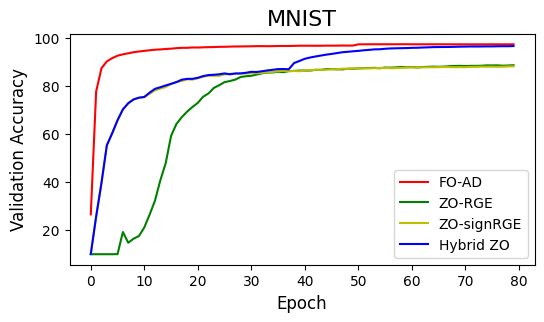
Figure 1: Validation accuracy of TT-MLPs trained by different optimizers on MNIST dataset. We set $N=10$ and $\mu=0.1$ in ZO-RGE, ZO-signRGE, and the coarse-tuning stage in hybrid ZO. We set $\mu=0.01$ and momentum $m=0.9$ in the fine-tuning stage in Hybrid ZO.

(2) Effectiveness of the Hybrid ZO Training.

Our hybrid ZO training was designed to achieve both good training accuracy and low function query complexity. To evaluate its effectiveness, we compare the hybrid ZO method with other baseline methods on the TT-MLP model with a compression ratio of $205\times$. Figure 1 shows the validation accuracy from different ZO optimizers. ZO-signRGE shows a more stable training than ZO-RGE at the beginning. However, both ZO-RGE and ZO-signRGE fail to achieve high accuracy in the late stage compared to the FO SGD baseline due to gradient estimation variance. With additional ZO-CGE fine-tuning, our hybrid ZO training strategy achieves a highly competitive result, comparable to the FO baseline. This hybrid ZO training optimizer balances the loss computation efficiency of ZO-signRGE and the accurate estimation capability of ZO-CGE. Specifically, to reach 85% accuracy in the early stage ZO-CGE needs 11 million forward evaluations while ZO-signRGE only needs 340K (32.75$\times$ fewer) forward evaluations. Table 2 presents the converged results of TT MLPs with different compression ratios. The advantage of the hybrid ZO over ZO-RGE and ZO-signRGE is consistent regardless of the compression ratio.

Method	Params	# of loss eval.	Best Acc.
Hybrid ZO Optimizer
HZO	814K	814K	83.58
TT-HZO (proposed)	4k	4K	96.64
SP-HZO	4k	4K	92.24
Sparse ZO Optimizer
FLOPS	814K	0.1K	83.50
STP	814K	24.4K	90.20*
SZO-SCD	814K	18.3K	93.50*
Forward Gradient
FG-W	272K	/	90.75
LG-FG-A	272K	/	96.76
FG-W	429K	/	91.44
LG-FG-A	429K	/	97.45
Feedback Alignment
FA	784K	/	97.90
DFA	1.26M	/	98.30

Table 3: Comparison of BP-free optimizers on the MNIST dataset. * means fine-tuning on a pre-trained model. In the Forward Gradient group, FG refers to forward gradient, LG refers to local objective functions added, -W refers to weight-perturbed, and -A refers to activity-perturbed.

(3) Comparison with other BP-free Training.

We further compare our TT-compressed hybrid ZO optimizer with three families of BP-free algorithms:

• Other ZO Optimizers: These methods use ZO optimization to estimate the gradients, and update model parameters with SGD iterations. Due to the dimension-dependent estimation error and loss computation complexity, most methods explore sparsity in training. FLOPS (Gu et al. 2020), STP (Bibi et al. 2020) and SZO-SCD (Gu et al. 2021a) assume a random pre-specified sparsity. We also extend the sparse method to ZO training.

• Forward Gradient (FG): Standard FG method uses forward-mode AD to evaluate the forward gradient and performs SGD-type iterations (Baydin et al. 2022). Ref. (Ren et al. 2022) further scales up this method by introducing activation perturbation and local loss to reduce the variance of forward gradient evaluation.

• Feedback Alignment (FA): Standard FA (Lillicrap et al. 2016) uses random and fixed backward weights. Direct feedback alignment (DFA) propagated the error through fixed random feedback connections directly from the output layer to each hidden layer. (Nøkland 2016).

The results are summarized in Table 3. For ZO optimizers, we also compare the number of loss computations needed for each iteration. Our method can achieve the best accuracy in weight perturbation-based methods. Compared with SOTA FG and FA algorithms, our method can also achieve comparable accuracy in the MNIST dataset. Note that our method contains over 107× fewer model parameters. This can greatly save the memory overhead for on-device training scenarios with restricted memory resources.

We remark that both FG and FA are not exactly black-box optimizers, since they rely on the computational graph of a given deep learning software. In practice, storing the computational graphs on an edge device can be expensive.

5.2 PINN for Solving High-Dim HJB PDE

We further use our BP-free method to train a PINN arising from high-dim optimal control of robots and autonomous systems. We consider the following 20-dim HJB PDE:

$$\partial_{t}u(\bm{x},t)+\Delta u(\bm{x},t)-0.05\left\|\nabla_{\bm{x}}u(\bm{x},t)\right\|_{2}^{2}=-2,$$ (14)

$$u(\bm{x},1)=\left\|\bm{x}\right\|_{1},\quad\bm{x}\in[0,1]^{20},~{}~{}t\in[0,1].$$

Here $\left\|\cdot\right\|_{p}$ denotes an $\ell_{p}$ norm. The exact solution is $u(\bm{x},t)=\left\|\bm{x}\right\|_{1}+1-t$. The baseline neural network is a 3-layer MLP ($21\times n,n\times n,n\times 1$, $n$ denotes the number of neurons in the hidden layer) with sine activation. We consider four options for computing derivatives in the loss: 1) finite-difference (FD) (Lim, Dutta, and Rotaru 2022), 2) Monte Carlo-based Stein Estimator (SE) (He et al. 2023), 3) our sparse-grid (SG) method, and 4) automatic differentiation (AD) as a golden reference. We approximate the solution $u_{\bm{\theta}}$ by a transformed neural network $f_{\bm{\theta}}^{{}^{\prime}}(\bm{x},t)=f_{\bm{\theta}}(\bm{x},t)+\left\|\bm{x}\right\|_{1}+1-t$, where $f_{\bm{\theta}}(\bm{x},t)$ is the base neural network or its TT-compressed version. Specifically, $u_{\bm{\theta}}(\bm{x},t)=f_{\bm{\theta}}^{{}^{\prime}}(\bm{x},t)$ for FD and AD, and $u_{\bm{\theta}}(\bm{x},t)=\mathbb{E}_{(\bm{\delta_{\bm{x}}},\delta_{t})\sim\mathcal{N}\left(\bm{0},\sigma^{2}\bm{I}\right)}f_{\bm{\theta}}^{{}^{\prime}}(\bm{x}+\bm{\delta_{\bm{x}}},t+\delta_{t})$ for SE and SG. Here the transformed network is designed to ensure that our approximated solution either exactly satisfies (FD, AD) or closely adheres to the terminal condition (SE, SG), allowing us to focus solely on minimizing the HJB residual during training.

In our hybrid ZO optimization, we set $\mu=0.1$ and $N=10$ in the ZO-signRGE coarse training stage. With greatly reduced variance by TT, ZO-signRGE can provide sufficiently accurate results, so fine-tuning is not necessary for this example. In the loss evaluation, we set the step size in FD to 0.01 and the noise level $\sigma$ to 0.1 in SE and SG. We use 1024 samples in SE and 925 samples in SG using a level-3 sparse Gaussian quadrature rule to approximate the expectations (8) and (9). Note that for most 2-dim or 3-dim PDEs, our SG method only requires $10\sim 30$ samples. Our results are summarized below:

• Effectiveness of BP-free loss computation: We compare our sparse-grid loss computation with those using AD, FD, and Monte Carlo-based Stein estimator, respectively. To evaluate different loss evaluations, we perform FO training and report the results in Table 4. The BP-free loss computation does not hurt the model performance, and our SG method is competitive compared to the original PINN training using AD for derivative computation.

• Evaluation of the BP-free PINN Training. Table 5 shows the MSE error of fully BP-free PINN training, using various BP-free loss computation and the proposed hybrid ZO training. By employing a tensor-train (TT) compressed model to reduce the variance, our method achieved a validation loss similar to standard FO training using AD. This observation clearly demonstrates that our method can bypass BP in both loss evaluation and model parameter updates with little accuracy loss.

• Comparison of dimensionality/variance reduction approaches. We compare our TT-compressed model with standard MLPs with dense fully connected (FC) layers and sparse-pruned (SP) MLPs in Table 6. For a fair comparison, all networks have similar model parameters. TT-compressed and SP model can reach better results than FC models as TT and SP can preserve the wide hidden layer. The SP model shows superior efficiency in FO training and achieves similar result with the TT model in ZO training. Note that the SP model only reduces the trainable parameters but not the model parameters, so TT models can achieve better memory and computation saving.

Network	Params	FO+AD	FO+FD	FO+SE	FO+SG
					(proposed)
MLP	608257	3.58E-04	5.97E-05	8.98E-04	4.27E-04
TT-MLP	7745	4.28E-05	4.90E-05	2.28E-04	7.14E-05
	3209	1.63E-05	4.56E-05	3.82E-04	4.49E-05

Table 4: FO training with different loss evaluations.

Network	Params	FO+AD	ZO+FD	ZO+SE	ZO+SG
					(proposed)
MLP	608257	3.58E-04	9.23E-02	diverge	1.62E-01
TT-MLP	7745	4.28E-05	3.79E-04	4.35E-04	4.79E-05
	3209	1.63E-05	3.82E-04	2.75E-04	1.44E-05

Table 5: ZO training results for 20-dim HJB PDE.

Network	Neurons	Params	FO-AD	ZO-SG
FC-3	768	608257	3.58E-04	1.62E-01
FC-3	78	7800	1.52E-02	4.35E-02
FC-2	320	7700	6.55E-04	1.00E-02
TT-3	768	7745	4.25E-05	4.79E-05
SP-3	768	7603	1.54E-09	6.29E-05

Table 6: Validation loss of various models for the HJB PDE

6 Relevant Work

Training on edge devices.

On-device inference has been well studied. However, training requires extra computation for BP and extra memory for intermediate results. Edge devices usually have tight memory and power budget, and run without an operating system, making it infeasible to implement modern deep learning frameworks that support automatic differentiation (Baydin et al. 2018). Most on-device training frameworks implemented BP by hand and only update within a small subspace (e.g., the last classifier layer (Donahue et al. 2014), biases (Zaken, Ravfogel, and Goldberg 2021), etc.), only capable of incremental learning or transfer learning by fine-tuning a pre-trained model. Some work leveraged pruning or sparse training to reduce the trainable parameter number(Lin et al. 2022; Gu et al. 2021b), but cannot achieve real memory savings. Recent work found tiny, trainable subspace exists in deep neural networks (Frankle and Carbin 2018; Li et al. 2022), but a pre-training is needed to identify such a subspace, which does not save the training overhead. Tensorized training  (Chen et al. 2021; Zhang et al. 2021) offers orders-of-magnitude memory reduction in the training process, enabling end-to-end neural network training on FPGA. However, it is non-trivial to implement this FO method to train larger models on edge devices due to the complex gradient computation.

Back-propagation-free training

Due to the complexity of performing BP on edge devices, several BP-free training algorithms have been proposed. These methods have gained more attentions in recent years as BP is also considered “biologically implausible”. ZO optimization (Ghadimi and Lan 2013; Duchi et al. 2015; Lian et al. 2016; Chen et al. 2019; Shamir 2017; Balasubramanian and Ghadimi 2022; Yang et al. 2020; Cai et al. 2021; Yang et al. 2023) plays an important role in tackling signal processing and machine learning problems, where actual gradient information is infeasible. For specific use cases, please refer to the survey by Liu et al. (2020a). ZO optimizations were also applied in on-device training for optical neural networks (ONN) (Gu et al. 2020, 2021a, 2021b). A ZO SGD-based method FLOPS (Gu et al. 2020) was proposed for end-to-end ONN training for vowel recognition, and a stochastic ZO sparse coordinate descent SZO-SCD (Gu et al. 2021a) was further proposed for efficient fine-tuning for ONN. But most ZO optimizations scale poorly when training real-size neural networks from scratch, due to their dimension-dependent gradient errors. Forward-forward algorithm was proposed for biologically plausible learning (Hinton 2022). Other BP-free training frameworks include the forward gradient method (Baydin et al. 2022), which updates the weights based on the directional gradient computed by forward-mode AD along a random direction. This method is further scaled up by leveraging activity perturbation and local loss for variance reduction(Ren et al. 2022). However, existing BP-free methods focus on training on HPC, lacking special concerns for the special challenges of on-device training. Furthermore, BP-free training of PINN remains an empty field.

7 Conclusion

Due to the high complexity and memory overhead of back propagations (BP) on edge devices, this paper has proposed a completely BP-free zeroth-order (ZO) approach to train real-size neural networks from scratch. Our method utilizes tensor compression to reduce the ZO gradient variance and a hybrid approach to improve the efficiency of ZO training. This has enabled highly accurate ZO training on the MNIST dataset, showing superior performance than sparse ZO approach. We have further extended this memory-efficient approach to train physics-informed neural networks (PINN) by developing a sparse-grid Stein gradient estimator for the loss evaluation. Our approach has been successfully solved a 20-dim HJB PDE, achieving similar accuracy with standard training using first-order optimization and automatic differentiation. Due to the huge memory reduction and the BP-free nature, our method can be easily implemented on various resource-constraint edge devices in the near future.

The ZO-CGE fine-tuning stage of our method requires many more function queries than the ZO-signRGE coarse-training stage. This prevents its applications in training large model (transformers) from scratch. We will address this issue in the future.

References

- Balasubramanian and Ghadimi (2022) Balasubramanian, K.; and Ghadimi, S. 2022. Zeroth-order nonconvex stochastic optimization: Handling constraints, high dimensionality, and saddle points. Foundations of Computational Mathematics, 1–42.
- Bansal and Tomlin (2021) Bansal, S.; and Tomlin, C. J. 2021. Deepreach: A deep learning approach to high-dimensional reachability. In 2021 IEEE International Conference on Robotics and Automation (ICRA), 1817–1824.
- Baydin et al. (2018) Baydin, A. G.; Pearlmutter, B. A.; Radul, A. A.; and Siskind, J. M. 2018. Automatic differentiation in machine learning: a survey. Journal of Marchine Learning Research, 18: 1–43.
- Baydin et al. (2022) Baydin, A. G.; Pearlmutter, B. A.; Syme, D.; Wood, F.; and Torr, P. 2022. Gradients without backpropagation. arXiv preprint arXiv:2202.08587.
- Berahas et al. (2022) Berahas, A. S.; Cao, L.; Choromanski, K.; and Scheinberg, K. 2022. A theoretical and empirical comparison of gradient approximations in derivative-free optimization. Foundations of Computational Mathematics, 22(2): 507–560.
- Bernstein et al. (2018) Bernstein, J.; Wang, Y.-X.; Azizzadenesheli, K.; and Anandkumar, A. 2018. signSGD: Compressed optimisation for non-convex problems. In International Conference on Machine Learning, 560–569. PMLR.
- Bibi et al. (2020) Bibi, A.; Bergou, E. H.; Sener, O.; Ghanem, B.; and Richtarik, P. 2020. A stochastic derivative-free optimization method with importance sampling: Theory and learning to control. In Proceedings of the AAAI Conference on Artificial Intelligence, volume 34, 3275–3282.
- Bolte and Pauwels (2020) Bolte, J.; and Pauwels, E. 2020. A mathematical model for automatic differentiation in machine learning. Advances in Neural Information Processing Systems, 33: 10809–10819.
- Cai et al. (2021) Cai, H.; Lou, Y.; McKenzie, D.; and Yin, W. 2021. A zeroth-order block coordinate descent algorithm for huge-scale black-box optimization. In International Conference on Machine Learning, 1193–1203. PMLR.
- Chen et al. (2017) Chen, P.-Y.; Zhang, H.; Sharma, Y.; Yi, J.; and Hsieh, C.-J. 2017. ZOO: Zeroth order optimization based black-box attacks to deep neural networks without training substitute models. In Proceedings of the 10th ACM workshop on artificial intelligence and security, 15–26.
- Chen et al. (2019) Chen, X.; Liu, S.; Xu, K.; Li, X.; Lin, X.; Hong, M.; and Cox, D. 2019. Zo-adamm: Zeroth-order adaptive momentum method for black-box optimization. Advances in neural information processing systems, 32.
- Chen et al. (2021) Chen, Y.; Hawkins, C.; Zhang, K.; Zhang, Z.; and Hao, C. 2021. 3U-EdgeAI: Ultra-low memory training, ultra-low bitwidth quantization, and ultra-low latency acceleration. In Proceedings of the 2021 on Great Lakes Symposium on VLSI, 157–162.
- Chiu et al. (2022) Chiu, P.-H.; Wong, J. C.; Ooi, C.; Dao, M. H.; and Ong, Y.-S. 2022. CAN-PINN: A fast physics-informed neural network based on coupled-automatic–numerical differentiation method. Computer Methods in Applied Mechanics and Engineering, 395: 114909.
- Donahue et al. (2014) Donahue, J.; Jia, Y.; Vinyals, O.; Hoffman, J.; Zhang, N.; Tzeng, E.; and Darrell, T. 2014. Decaf: A deep convolutional activation feature for generic visual recognition. In International conference on machine learning, 647–655. PMLR.
- Duchi et al. (2015) Duchi, J. C.; Jordan, M. I.; Wainwright, M. J.; and Wibisono, A. 2015. Optimal rates for zero-order convex optimization: The power of two function evaluations. IEEE Transactions on Information Theory, 61(5): 2788–2806.
- Frankle and Carbin (2018) Frankle, J.; and Carbin, M. 2018. The lottery ticket hypothesis: Finding sparse, trainable neural networks. arXiv preprint arXiv:1803.03635.
- Garcke et al. (2006) Garcke, J.; et al. 2006. Sparse grid tutorial. Mathematical Sciences Institute, Australian National University, Canberra Australia, 7.
- Gerstner and Griebel (1998) Gerstner, T.; and Griebel, M. 1998. Numerical integration using sparse grids. Numerical algorithms, 18(3-4): 209.
- Ghadimi and Lan (2013) Ghadimi, S.; and Lan, G. 2013. Stochastic first-and zeroth-order methods for nonconvex stochastic programming. SIAM Journal on Optimization, 23(4): 2341–2368.
- Gu et al. (2021a) Gu, J.; Feng, C.; Zhao, Z.; Ying, Z.; Chen, R. T.; and Pan, D. Z. 2021a. Efficient on-chip learning for optical neural networks through power-aware sparse zeroth-order optimization. In Proceedings of the AAAI Conference on Artificial Intelligence, volume 35, 7583–7591.
- Gu et al. (2020) Gu, J.; Zhao, Z.; Feng, C.; Li, W.; Chen, R. T.; and Pan, D. Z. 2020. FLOPS: EFficient On-Chip Learning for OPtical Neural Networks Through Stochastic Zeroth-Order Optimization. In 2020 57th ACM/IEEE Design Automation Conference (DAC), 1–6.
- Gu et al. (2021b) Gu, J.; Zhu, H.; Feng, C.; Jiang, Z.; Chen, R.; and Pan, D. 2021b. L2ight: Enabling on-chip learning for optical neural networks via efficient in-situ subspace optimization. Advances in Neural Information Processing Systems, 34: 8649–8661.
- Hawkins, Liu, and Zhang (2022) Hawkins, C.; Liu, X.; and Zhang, Z. 2022. Towards compact neural networks via end-to-end training: A bayesian tensor approach with automatic rank determination. SIAM Journal on Mathematics of Data Science, 4(1): 46–71.
- Hawkins and Zhang (2021) Hawkins, C.; and Zhang, Z. 2021. Bayesian tensorized neural networks with automatic rank selection. Neurocomputing, 453: 172–180.
- He et al. (2023) He, D.; Li, S.; Shi, W.; Gao, X.; Zhang, J.; Bian, J.; Wang, L.; and Liu, T.-Y. 2023. Learning physics-informed neural networks without stacked back-propagation. In International Conference on Artificial Intelligence and Statistics, 3034–3047. PMLR.
- Hinton (2022) Hinton, G. 2022. The forward-forward algorithm: Some preliminary investigations. arXiv preprint arXiv:2212.13345.
- Lagaris, Likas, and Fotiadis (1998) Lagaris, I. E.; Likas, A.; and Fotiadis, D. I. 1998. Artificial neural networks for solving ordinary and partial differential equations. IEEE transactions on neural networks, 9(5): 987–1000.
- Li et al. (2022) Li, T.; Tan, L.; Huang, Z.; Tao, Q.; Liu, Y.; and Huang, X. 2022. Low dimensional trajectory hypothesis is true: Dnns can be trained in tiny subspaces. IEEE Transactions on Pattern Analysis and Machine Intelligence, 45(3): 3411–3420.
- Lian et al. (2016) Lian, X.; Zhang, H.; Hsieh, C.-J.; Huang, Y.; and Liu, J. 2016. A comprehensive linear speedup analysis for asynchronous stochastic parallel optimization from zeroth-order to first-order. Advances in Neural Information Processing Systems, 29.
- Lillicrap et al. (2016) Lillicrap, T. P.; Cownden, D.; Tweed, D. B.; and Akerman, C. J. 2016. Random synaptic feedback weights support error backpropagation for deep learning. Nature communications, 7(1): 13276.
- Lim, Dutta, and Rotaru (2022) Lim, K. L.; Dutta, R.; and Rotaru, M. 2022. Physics informed neural network using finite difference method. In 2022 IEEE International Conference on Systems, Man, and Cybernetics (SMC), 1828–1833. IEEE.
- Lin et al. (2022) Lin, J.; Zhu, L.; Chen, W.-M.; Wang, W.-C.; Gan, C.; and Han, S. 2022. On-device training under 256kb memory. Advances in Neural Information Processing Systems, 35: 22941–22954.
- Liu et al. (2019) Liu, S.; Chen, P.-Y.; Chen, X.; and Hong, M. 2019. signSGD via zeroth-order oracle. In International Conference on Learning Representations.
- Liu et al. (2020a) Liu, S.; Chen, P.-Y.; Kailkhura, B.; Zhang, G.; Hero III, A. O.; and Varshney, P. K. 2020a. A primer on zeroth-order optimization in signal processing and machine learning: Principals, recent advances, and applications. IEEE Signal Processing Magazine, 37(5): 43–54.
- Liu et al. (2020b) Liu, S.; Lu, S.; Chen, X.; Feng, Y.; Xu, K.; Al-Dujaili, A.; Hong, M.; and O’Reilly, U.-M. 2020b. Min-max optimization without gradients: Convergence and applications to black-box evasion and poisoning attacks. In International conference on machine learning, 6282–6293. PMLR.
- Malladi et al. (2023) Malladi, S.; Gao, T.; Nichani, E.; Damian, A.; Lee, J. D.; Chen, D.; and Arora, S. 2023. Fine-Tuning Language Models with Just Forward Passes. arXiv preprint arXiv:2305.17333.
- McMahan et al. (2017) McMahan, B.; Moore, E.; Ramage, D.; Hampson, S.; and y Arcas, B. A. 2017. Communication-efficient learning of deep networks from decentralized data. In Artificial intelligence and statistics, 1273–1282. PMLR.
- Nesterov and Spokoiny (2017) Nesterov, Y.; and Spokoiny, V. 2017. Random gradient-free minimization of convex functions. Foundations of Computational Mathematics, 17: 527–566.
- Nobile, Tempone, and Webster (2008) Nobile, F.; Tempone, R.; and Webster, C. G. 2008. A sparse grid stochastic collocation method for partial differential equations with random input data. SIAM Journal on Numerical Analysis, 46(5): 2309–2345.
- Nøkland (2016) Nøkland, A. 2016. Direct feedback alignment provides learning in deep neural networks. Advances in neural information processing systems, 29.
- Onken et al. (2021) Onken, D.; Nurbekyan, L.; Li, X.; Wu Fung, S.; Osher, S.; and Ruthotto, L. 2021. A Neural Network Approach Applied to Multi-Agent Optimal Control. In European Control Conference.
- Oseledets (2011) Oseledets, I. V. 2011. Tensor-train decomposition. SIAM Journal on Scientific Computing, 33(5): 2295–2317.
- Polyak (1964) Polyak, B. T. 1964. Some methods of speeding up the convergence of iteration methods. Ussr computational mathematics and mathematical physics, 4(5): 1–17.
- Raissi, Perdikaris, and Karniadakis (2019) Raissi, M.; Perdikaris, P.; and Karniadakis, G. E. 2019. Physics-informed neural networks: A deep learning framework for solving forward and inverse problems involving nonlinear partial differential equations. Journal of Computational physics, 378: 686–707.
- Ren et al. (2022) Ren, M.; Kornblith, S.; Liao, R.; and Hinton, G. 2022. Scaling forward gradient with local losses. arXiv preprint arXiv:2210.03310.
- Rumelhart, Hinton, and Williams (1986) Rumelhart, D. E.; Hinton, G. E.; and Williams, R. J. 1986. Learning representations by back-propagating errors. nature, 323(6088): 533–536.
- Shamir (2017) Shamir, O. 2017. An optimal algorithm for bandit and zero-order convex optimization with two-point feedback. The Journal of Machine Learning Research, 18(1): 1703–1713.
- Stein (1981) Stein, C. M. 1981. Estimation of the mean of a multivariate normal distribution. The annals of Statistics, 1135–1151.
- Sun, Jha, and Fan (2020) Sun, D.; Jha, S.; and Fan, C. 2020. Learning certified control using contraction metric. arXiv preprint arXiv:2011.12569.
- Sutskever et al. (2013) Sutskever, I.; Martens, J.; Dahl, G.; and Hinton, G. 2013. On the importance of initialization and momentum in deep learning. In International conference on machine learning, 1139–1147. PMLR.
- Wang, Zhang, and Grosse (2020) Wang, C.; Zhang, G.; and Grosse, R. 2020. Picking winning tickets before training by preserving gradient flow. arXiv preprint arXiv:2002.07376.
- Wasilkowski and Wozniakowski (1995) Wasilkowski, G. W.; and Wozniakowski, H. 1995. Explicit cost bounds of algorithms for multivariate tensor product problems. Journal of Complexity, 11(1): 1–56.
- Xiang et al. (2022) Xiang, Z.; Peng, W.; Zhou, W.; and Yao, W. 2022. Hybrid finite difference with the physics-informed neural network for solving pde in complex geometries. arXiv preprint arXiv:2202.07926.
- Yang et al. (2023) Yang, Y.; Chen, L.; Zhou, P.; and Ding, X. 2023. Vflh: A following-the-leader-history based algorithm for adaptive online convex optimization with stochastic constraints. Available at SSRN 4040704.
- Yang et al. (2020) Yang, Y.; Xu, J.; Xu, Z.; Zhou, P.; and Qiu, T. 2020. Quantile context-aware social IoT service big data recommendation with D2D communication. IEEE Internet of Things Journal, 7(6): 5533–5548.
- Yu et al. (2023) Yu, X.; Serrallés, J. E.; Giannakopoulos, I. I.; Liu, Z.; Daniel, L.; Lattanzi, R.; and Zhang, Z. 2023. PIFON-EPT: MR-Based Electrical Property Tomography Using Physics-Informed Fourier Networks. arXiv preprint arXiv:2302.11883.
- Zaken, Ravfogel, and Goldberg (2021) Zaken, E. B.; Ravfogel, S.; and Goldberg, Y. 2021. Bitfit: Simple parameter-efficient fine-tuning for transformer-based masked language-models. arXiv preprint arXiv:2106.10199.
- Zhang et al. (2021) Zhang, K.; Hawkins, C.; Zhang, X.; Hao, C.; and Zhang, Z. 2021. On-FPGA training with ultra memory reduction: A low-precision tensor method. arXiv preprint arXiv:2104.03420.
- Zhang et al. (2022) Zhang, Y.; Yao, Y.; Jia, J.; Yi, J.; Hong, M.; Chang, S.; and Liu, S. 2022. How to Robustify Black-Box ML Models? A Zeroth-Order Optimization Perspective. In International Conference on Learning Representations.