SICO: Simulation for Infection Control Operations

https://www.frontiersin.org/articles/10.3389/fitd.2021.707865/full

Abstract

In response to the COVID-19 pandemic and the potential threat of future epidemics caused by novel viruses, we developed a flexible framework for modeling disease intervention effects. This tool is intended to aid decision makers at multiple levels as they compare possible responses to emerging epidemiological threats for optimal control and reduction of harm. The framework is specifically designed to be both scalable and modular, allowing it to model a variety of population levels, viruses, testing methods and strategies–including pooled testing–and intervention strategies. In this paper, we provide an overview of this framework and examine the impact of different intervention strategies and their impact on infection dynamics.

supp

[l1]organization=Matrix Research, addressline=3844 Research Blvd., city=Beavercreek, postcode=45430, state=OH,country=USA [l2]organization=Keystone Strategy LLC, addressline=116 Huntington Ave., city=Boston, state=MA, postcode=02116, country=USA [l3]organization=Möbius Logic, addressline=1775 Tysons Blvd., city=Tysons, state=VA, postcode=22102, country=USA

1 Introduction

COVID-19 emerged from obscurity and rapidly became the most destructive event of the century. The death toll currently stands at nearly 7 million lives lost [1]. The economic impact exceeds 3.9% of the median global GDP [2] and is expected to slow global economic recovery for the next several years. The societal costs of lockdowns and stay-at-home orders will be years manifesting. To achieve and maintain a sense of normalcy in the wake of COVID-19, we must find methods to surveil emerging variants and limit further transmission, thereby preventing additional waves of infection and potential lockdown situations. Moving forward from COVID-19, our goal is resiliency against future pandemics [3] with the development of flexible technologies that can be adapted to different disease and population characteristics. Expedient modeling of infectious disease transmission mitigation measures can inform decision makers in the critical early days of infection spread.

The work of Lyng et al. [4] and Augenblick et al. [5] has demonstrated the importance of modeling many combinations of testing and intervention strategies over time. Additionally, a dynamic approach to modeling is needed as infection rates and population characteristics fluctuate. In practice, the disease management problem is complex, with many possible population-dependent intervention alternatives. Therefore, it is necessary to model many aspects of infection and population dynamics to effectively determine an ideal disease control strategy. We address this need with the creation of our Simulation for Infection Control Operations (SICO) that allows users to explore alternative planning and testing scenarios, adapting situational parameters such as vaccination rate, isolation, and testing with customization based on the disease scenario being considered. The tool is built utilizing an agent-based model (ABM) which provides flexibility in specifying the disease dynamics, test availability, and economic constraints important for its application in the management of future pandemics [3]. The use of an ABM allows SICO to account for variations in agent behaviors, such as propensity to vaccinate and likelihood to self-isolate upon symptoms. Further, SICO uses a stochastic ABM to simulate various infectious disease intervention strategies—thus enabling a decision maker to choose an optimal strategy for long-term disease reduction which adheres to any physical constraints (e.g. test or vaccine availability) they face.

In introducing SICO, our contribution to the field is developing a hybrid epidemilogical ABM with a flexible, compartmentalized and modular design which allows it to be adapted and customized to fit a variety of infectious diseases, disease propagation scenarios and intervention strategies. Some noteworthy features of SICO include:

• Ability to model various vaccination strategies based on vaccine supply and individual agents’ propensity to vaccinate;

• Ability to model a large variety of testing strategies (including pooled testing strategies) based on test availability, test cost, and test accuracy and sensitivity;

• Option for a user to specify a custom stochastic viral load profile which is used to determine an exposed agent’s trajectory within the model;

• Separate vaccinated and unvaccinated susceptible states;

• Ability to separately track isolated agents based on whether they were isolated due to a false or true positive infection test;

• Ability to model loss of immunity by recovered agents; and

• Flexible agent trajectories (for example, an infectious agent does not need to be isolated before it can become recovered).

This paper is organized as follows: Related work expands on current designs in high-frequency and pooled testing, with primary emphasis given to work that combines both or acknowledges real-world limitations and complications of applied testing. Next, Model design elaborates on choices made in the model design, involving the disease model and propagation, implementation of testing procedures, the impact of immunization, and cost estimation. Then, Experimental setup and Results demonstrate the flexibility and utility of SICO by examining validation sims and their impact on model performance for multiple specific infectious disease transmission scenarios and corresponding mitigation strategies. We demonstrate reduced infection with more-rapid testing or test turnaround, diminished rates of false positives (and thus false isolation of healthy individuals) with pooled testing, and the robustness of these results under varied vaccination regimes. Finally, we conclude with suggested applications of SICO and potential avenues for future improvement.

2 Related work

In the monitoring of COVID-19, molecular assays are an important tool for detecting symptomatic and asymptomatic infections and have played a vital role [6, 7]. Quantitative real-time polymerase chain reaction (qRT-PCR) testing has been the gold standard for clinical diagnosis, due to the high sensitivity and specificity, but is expensive, requires highly-trained technicians, and incurs longer turn-around times [8]. The expense and skilled workers required for qRT-PCR testing inhibits its application in resource-limited settings and in large-scale population screening. The delay between testing and reporting allows presymptomatic or asymptomatic individuals to spread COVID-19 prior to isolation. Because of these difficulties, several studies have suggested methods for reducing cost or improving response time of testing [9, 10, 5, 4, 11, 12].

Suggestions for population-level screening have followed two prongs: high-frequency testing using low-cost tests [11, 12] or pooled testing to increase the cost ratio of qRT-PCR tests [10, 5]. A problem with antigen tests is lowered sensitivity [13], however, this is made up for by vastly reduced response time [11]. Pooled testing maintains the sensitivity of qRT-PCR, and increases the efficiency of testing in low-endemic scenarios [5], but is often accompanied by complicated pooling designs intended to optimize the one-shot throughput of testing [10, 14]. Two groups in particular [5, 4] have attempted to marry these two prongs—combining pooled testing with higher-frequency test application to combat costs and result turn-around time. While no method has been superior to all others under all constraints, this is a promising direction that combines the strengths of both methods and provides an opportunity to adapt testing protocols as infection rates fluctuate [15, 16].

Continued testing of large cohorts, such as schools and businesses, for surveillance and prevention of pandemics is complicated and potentially prohibitively expensive. Testing regimens must be designed to minimize spread and reduce infection rates while also being simple and cheap enough to maintain for weeks or months on end [17, 18]. Towards this end, several studies have explored methods for curbing COVID-19 spread in the face of social re-openings [19, 4, 12, 5, 9].

Most simulation studies have focused on one of two options for disease transmission mitigation: high-frequency testing or pooled testing. Proponents of high-frequency testing [11, 9, 20, 21] advocate for the distribution of antigen-based self-testing methods. These tests have lower sensitivity and specificity than qRT-PCR tests, but are significantly cheaper and have a turn-around time of minutes [22, 23, 24]. Proponents of pooled testing [10, 14, 25, 26, 27] devise methods to use the sensitivity of qRT-PCR as an advantage, increasing the efficiency of individual tests. These studies predominantly implement two-stage Dorfman testing [28] and generate complicated pooling designs. However, both options have shortcomings: the lack of sensitivity in antigen tests reduces their detection of asymptomatic or presymptomatic individuals, while complicated pooling designs are hard to adhere to in practice and ignore the repetitive nature of testing (frequent testing would make learning/implementing complicated pooling designs more robust).

Lyng et al. [4] and Augenblick et al. [5] demonstrate the importance of modeling intervention strategies in conjunction, finding a hybrid high-frequency pooled testing approach to be more effective than either strategy alone. The latter [5] takes a theoretical approach, demonstrating enhanced efficiency in pooling designs through reduction in disease prevalence over time. While highly compelling, their simplified disease model and lack of tool make it hard to apply their results in practice.  Lyng et al. [4] implement a stochastic, compartmental SIR disease model to explore pooling, frequency of testing, testing delays, as well as optimize for cost and sensitivity/specificity of tests. Both approaches demonstrate the benefits of a hybrid design, but suffer from simplistic disease models and time-invariant testing and pooling strategies.

SICO extends these works [4, 5] in several key ways. For a more complete simulation of the disease dynamics we extend the model to include other interventions, such as isolation and vaccination. This is reflected in a descriptive disease model, accounting for asymptomatic, presymptomatic, isolated, recovered, and imported infections using an agent-based model. Additionally, we implement custom viral load dynamics for all infected individuals, using methods from Cleary et al. [15] and Larremore et al. [11]. We maintain ideas from Lyng et al. [4] and explore the impact of test sensitivity, specificity, response time, and frequency. Finally, we provide all of this in a modular and computationally-efficient tool. These extensions provide users with the ability to simulate a much larger array of hybrid interventions on populations with a variety of characteristics. Additionally, the modularity allows expert users to adapt and extend our work to novel diseases [3] or population structures. The model’s efficiency allows for users to simulate many disease control scenarios quickly and update them as new information becomes available.

The epidemiological model SICO is based on is similar in concept to the Generalized SEIR model introduced by Liangrong Peng et al. in 2020 and added to the MATLAB code base later that same year by E. Cheynet [29, 30]. Despite the apparent similarities, SICO represents a significant extension of Generalized SEIR in terms of both flexibility and functionality. A summary comparison of SICO with Generalized SEIR is provided in E.

3 Model design

SICO is built on an agent-based model in which each agent is assigned a set of individual parameters to account for diversity in the population. This type of model provides flexibility to vary transitions between states based on individual characteristics such as vaccination status, viral load, and likelihood of self-isolation. States that agents can occupy are based on an enhanced SIR compartmental model. This set-up allows for the easy removal or addition of modules or compartments based on scenario characteristics. The currently implemented model includes modules to simulate testing, isolation, vaccination, and disease progression in terms of viral load and status of symptoms. All parameters associated with the various modules listed below are included in A.

3.1 Epidemiological model

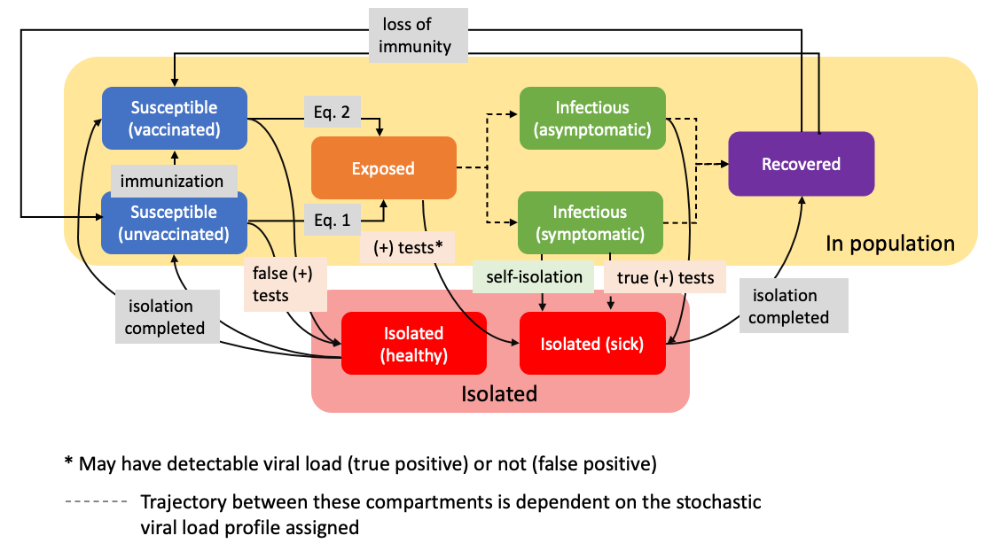
Figure 1: Compartmental model. Agents move between six compartments in the population (susceptible, exposed, infectious and recovered) and two compartments removed from the population (isolated while healthy or sick). The probability that a susceptible individual is exposed to the disease each day is given by Eq. 1 or Eq. 2, depending on their vaccination status. Once exposed, an individual’s disease trajectory is determined by their viral load profile. A positive test at any point places an agent in isolation with “healthy” or “sick” status determined by their infection status. Additionally, agents who are experiencing symptoms may choose to isolate based on their pre-designated propensity to isolation on symptoms.

Agents in the simulation move between six disjoint compartments following a variation of the SIR disease propagation model. We distinguish between when an agent is within the population versus when it is isolated from the population for easier computation of the disease propagation. Possible states within the population include:

• Susceptible (vaccinated, $S_{v}$, or unvaccinated, $S_{u}$): A susceptible agent has the ability to be infected. The number of susceptible agents is given by the sum of unvaccinated susceptible and vaccinated susceptible, $S=S_{v}+S_{u}$.

• Exposed, $E$: An agent is in the exposed category if it is infected but not yet infectious (based on a preset viral load infectiousness threshold).

• Infectious (symptomatic, $I_{s}$, or asymptomatic, $I_{a}$): An exposed agent becomes a infectious agent once its viral load surpasses the designated infectiousness threshold. An infectious agent can be either symptomatic or asymptomatic, $I=I_{s}+I_{a}$.

• Recovered, $R$: An agent has recovered once its viral load falls below the infectiousness threshold.

The total number of agents in the population (not in isolation) at a given time is given by $P=S+E+I+R$. Additionally, if an agent is isolated it is in either the isolated (healthy) or isolated (sick) state, where the isolated (healthy) state is comprised of agents who received a false positive test result.

3.1.1 Exposure

The probability that an unvaccinated susceptible agent is exposed to the disease on a given day is given by the sum of the probability an agent is exposed outside the population and the mass action probability of being exposed inside the population:

$$\mathbb{P}(S_{u}\rightarrow E)=\gamma+\beta\frac{I}{P},$$ (1)

where $\gamma$ is the probability of being infected outside the population and $\beta$ is the typical interaction parameter. We assume a well-mixed population and randomly choose $\mathbb{P}(S_{u}\rightarrow I)\cdot S_{u}$ of the $S_{u}$ susceptible agents to be exposed.

The exposure process for vaccinated susceptible agents is similar to (1), with the addition of a immunity discount factor, $\alpha$:

$$\mathbb{P}(S_{v}\rightarrow E)=\alpha\left(\gamma+\beta\frac{I}{P}\right).$$ (2)

As in the previous case, $\mathbb{P}(S_{v}\rightarrow E)\cdot S_{v}$ are randomly chosen from $S_{v}$ to become exposed.

3.1.2 Viral load progression

The progression of disease transmissibility and symptoms is characterized by the disease and can be highly variable between individuals [31]. For the COVID-19 based scenarios explored in Sections 4 and 5, we demonstrate SICO’s ability to utilize a user specified viral load evolution model by implementing one based on the work of Larremore et al. [11]. This models the viral load as having a hinge-function profile (consistent with Marc et al. [32]) with variations between asymptomatic and symptomatic individuals.

At the time of exposure, the newly exposed individuals are chosen to be symptomatic or asymptomatic with probability $\sigma_{s}$ (A.2: fractionSymptomatic). An agent is assigned a set of viral load parameters chosen from the corresponding distributions (described below and summarized in Table 1). The resulting viral load progression influences an agent’s progression from exposed $\rightarrow$ infectious (symptomatic or asymptomatic) $\rightarrow$ recovered. Additionally, an agent’s viral load directly affects the results of any testing that may take place during this period. The structure of this module and distribution of parameters can be modified to model the progression of a different disease.

Parameter	Distribution	Description
$\sigma_{s}$	0.5	Probability of an agent being symptomatic
$t_{0}$	$\text{uniform}(2.5,3.5)$	Time interval of viral load initialization
$V_{0}$	$10^{3}$ cp/ml	Initial viral load
$t_{P}$	$\Gamma(1.5,1)+0.5$	Time interval to achieve peak viral load
$V_{P}$	$\text{uniform}(10^{4},10^{7})$	Peak viral load
$t_{S}$	$\text{uniform}(0,3)$	Time interval for symptoms to begin
$t_{F}$	$\text{uniform}(4,9)$	Time interval for viral load to decline to $V_{F}$ level
$V_{F}$	$10^{3}$ cp/ml	Final viral load level
$V_{I}$	$10^{3}$ cp/ml	Minimum viral load for infectiousness

Table 1: Viral load parameters and their corresponding distributions.

The asymptomatic viral-load trajectory is a hinge-function defined by the (time (days), viral load (cp/ml)) coordinates:

$$(t_{0},V_{0})\rightarrow(t_{0}+t_{P},V_{P})\rightarrow(t_{0}+t_{P}+t_{F},V_{F}),$$ (3)

where each variable is drawn from the distributions in Table 1. The trajectory for a symptomatic individual is similar, with the addition of the appearance of symptoms $t_{S}$ days after achieving peak viral load. This also results in a prolonged decrease of viral load back to the initial baseline. The function coordinates are:

$$(t_{0},V_{0})\rightarrow(t_{0}+t_{P},V_{P})\rightarrow(t_{0}+t_{P}+t_{S}+t_{F},V_{F}).$$ (4)

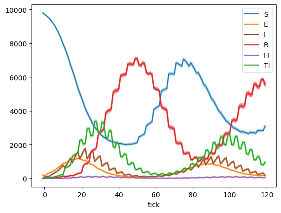
(c) 4 day testing interval, pool size 5.

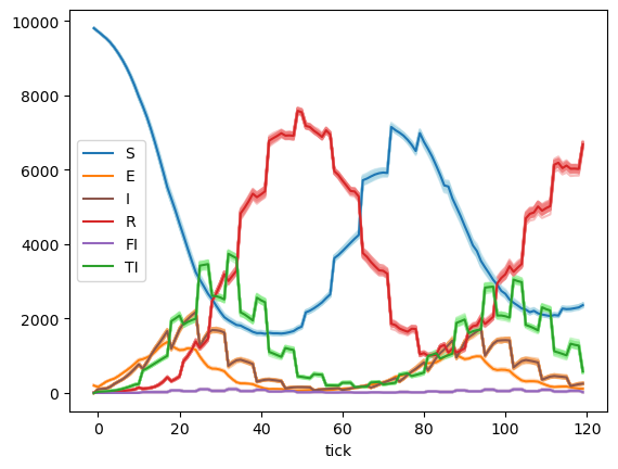
(d) 7 day testing interval, pool size 5.

Figure 2: Vaccination A (no vaccination) + Test A. Subfigures show the number of individuals in the population occupying each of the disease model compartments (susceptible, exposed, infectious, recovered, falsely isolated, and isolated while transmitting). Plots for all 50 runs of each scenario are overlayed on the corresponding subfigure with the average of each compartment over all runs shown in a darker shade.

This process along with fifty resulting viral load profiles is shown in Fig. 2.

Once an agent’s viral load reaches a user designated threshold for infectiousness (A.2: infectiousViralLoadCut ($V_{I}$)) it is moved from exposed to either infectious (symptomatic) or infectious (asymptomatic). Similarly, once an infectious agent’s viral load drops below the infectiousness threshold, the agent is moved to recovered. If $V_{0}=V_{F}=V_{I}$ the total time an asymptomatic (symptomatic) agent is infectious is $t_{0}+t_{P}+t_{F}$ ($t_{0}+t_{P}+t_{S}+t_{F}$).

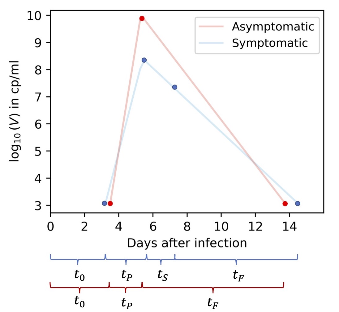
(a) Viral load model.

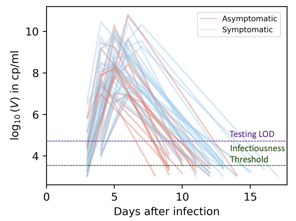
(b) Example viral load profiles.

Figure 2: Viral load model. Description and example trajectories associated with the viral load model based on that of Larremore et al. [11]. Note that although panel 2(a) shows the asymptomatic trajectory achieving a higher viral load than the symptomatic trajectory, in general this is not the case. These are two sample trajectories from the stochastic process based on the distributions in Table 1.

3.2 Population interventions

3.2.1 Testing

One of the most common types of interventions for infectious disease transmission mitigation is population testing. The numerous types of tests, schedules, and costs involved make this a key process for decision makers to optimize. These types of decisions often have multiple objectives as employers wish to limit the spread of disease while also limiting the cost and mental health impact associated with unnecessary isolation resulting from false positive tests. Our simulation is able to quickly compare many scenarios and can be used to inform disease control decisions.

We offer users the ability to specify parameters for test schedule (initial day of testing and testing frequency) and optionally for two-stage Dorfman pooling (pool size and function to use for determining pooled test outcome). Different types of tests can also be compared by setting the viral load threshold at which the disease can be detected, as well as a false negative rate, false positive rate, and delay for the return of test results. See the full list of testing parameters in A.3.

When testing is performed, all eligible individuals are split into pools of the designated size. If a pool consists of a single individual, then single testing is performed, otherwise we use a two-stage Dorfman pooled testing procedure [28].

In the single sample testing procedure, each individual $i$ is considered detectable if their viral load ($v_{i}$) is greater than test $m$’s limit of detection ($l_{m}$). The single sample testing result $t_{m}(i)$ of sample $i$ is then positive with probability:

$$\mathbb{P}\big{(}t_{m}(i)=+\big{)}=\begin{cases}\phi_{p}&v_{i}\leq l\\ 1-\phi_{n}&v_{i}>l\end{cases},$$ (5)

where $\phi_{p}$ and $\phi_{n}$ are the false positive and false negative rates associated with the test.

The two-stage Dorfman pooled testing procedure is similar to that of the single testing procedure, but proceeded by a test applied to each pool. We offer users two functions for determining the pooled test results, average pooling and exponential pooling. Both are defined in A.3:poolingType, but we limit the discussion here to the default option, average pooling. We use an apostrophe to distinguish the viral load and testing result of a pool ($v^{\prime}_{j}$, $t^{\prime}(j)$) from that of a single sample ($v_{i}$, $t(i)$).

In this case, the viral load content of a pool $j$ is defined as the average of the viral load of all samples in the pool. That is,

$$v^{\prime}_{j}=\displaystyle\sum_{i=1}^{N}v_{i}/N,$$ (6)

where $N$ is the size of the pool. As above, a pool is considered detectable if the viral load, $v^{\prime}_{j}$, is greater than the test’s limit of detection. The probability that pool $j$’s test result, $t^{\prime}_{m}(j)$, is positive is,

$$\mathbb{P}\big{(}t^{\prime}_{m}(j)=+\big{)}=\begin{cases}\phi_{p}&v^{\prime}_{j}\leq l\\ 1-\phi_{n}&v^{\prime}_{j}>l\end{cases}.$$ (7)

After testing each pool (stage 1), the second stage consists of applying single sample testing to every member of each positive pool.

3.2.2 Isolation

Isolation procedures and self-isolation play a key role in removing infectious individuals from a population. We consider two cases of isolation: isolation due to receipt of positive testing results or self-isolation due to experiencing symptoms. We assume agents in the first case are entirely compliant as this may be enforceable by an employer, testing official, etc. Isolation parameters in this simulation include length of isolation and the probability that agents self-isolate when symptoms are experienced. Additionally, users may choose to enact the withholding of tests for a set period of time after agents have exited isolation and recovered. The full list of isolation parameters are included in A.4.

In the case of an agent testing positive, if they are exposed or infectious at the time of testing positive, they are moved to the isolation (sick) compartment. If the agent is susceptible at the time of testing (i.e. they tested positive falsely), they are moved to the isolation (healthy) compartment. Additionally, when an agent experiences symptoms, they may choose to self-isolate based on the preset probability of self-isolation. These individuals are also moved to the isolation (sick) compartment.

After a set number of days, agents in the isolation (sick) compartment are moved to recovered. Likewise, individuals in the isolation (healthy) compartment are moved back to susceptible.

3.2.3 Vaccination

Once a vaccine has been developed for an infectious disease, immunization of a population is one of the most effective methods of reducing the impact of an infectious disease. In this simulation users are able to simulate the distribution of vaccines by specifying the rate at which vaccines are available to the population. Agents’ preferences can also be modeled by specifying a distribution of vaccine acceptance among agents. In this case agent $i$ is assigned a “willingness to vaccinate” probability, $\nu_{i}$, between 0 and 1 drawn from the distribution. At each time step, $t$, agents are labeled as “willing” to vaccinate with probability:

$$\mathbb{P}(\text{agent $i$ is willing to vaccinate during time step $t$})=\nu_{i}.$$ (8)

The vaccines that are available are distributed to the willing agents until all willing agents have been vaccinated. See A.5 for the full list of vaccination parameters.

3.3 Ordering of simulation procedures

All simulation processes are described above in detail, but for completeness, we also include here the order in which each of these processes takes place during a single simulation time step or “day.”

1. External exposure: The first stage of the simulation records exposure that occurred outside the population (the first term in Eqs. 1 and 2). Exposed agents are labeled as symptomatic or asymptomatic and assigned a set of viral load parameters according to Section 3.1.2. At this point the full viral load timeline is also saved for easy reference throughout the simulation.

2. Update agent status: This stage encompasses the bulk of agent movement between compartments and parameter updates. This includes:

   • Advancing the viral load of each exposed and infectious agent by one time step

   • Movement of agents between compartments based on any testing results received on this day

   • Agents’ exit from isolation if they have completed the designated number of days

   • Movement from exposed to infectious for any agents with viral load above the infectiousness threshold

   • Movement from recovered to susceptible based on the number of days since each agent’s recovery

3. Self-isolation: A subset of the agents which are symptomatic are placed into isolation based on the propensity to self-isolate parameter.

4. Testing: If the current time step is designated as a testing day, samples are pooled (if applicable) and testing is performed. Results are scheduled to be received in the future based on the parameter delaying test results.

5. Infection propagation: Agents are infected based on exposure in the population (second term of Eqs. 1 and 2). Again, agents are marked as symptomatic or asymptomatic and assigned a viral load timeline.

6. Vaccination: Eligible agents (not in isolation and not yet vaccinated) are chosen for vaccination based on the number of available vaccines and each agent’s propensity to vaccinate.

3.4 Implementation

SICO is implemented in Python and features scripts for duplicating results from this paper as well as creating new disease scenarios. Many parameters are dependent on the disease and population being modeled, and thus we leave their selection to the researchers and decision-makers with knowledge of the specifics. However, some general strategies for estimating population parameters such as “propensity to isolate” may be to provide a survey to employees or estimate from the general public. The simulations performed in Section 4 took around 6 seconds per scenario using a single CPU.

4 Experimental setup

Capabilities of SICO were demonstrated through a series of simulations. Our goal was to showcase scenarios where the tool could be used to evaluate alternative courses of action for management of a disease in a population. Disease dynamics for a simulated population of 10,000 agents were examined for a variety of vaccination and testing scenarios. To our knowledge, no non-healthcare business provided vaccines for COVID-19, and thus our simulations assume an exogenous application and uptake of vaccines in the population. Three different vaccination scenarios (Table 2) loosely represent dynamics in a population without any vaccination (Vaccination A), during vaccine rollout in an unvaccinated population (Vaccination B), or during continued vaccine distribution in a partially vaccinated population (Vaccination C).

Within each of these vaccination settings the effect of several testing schemes were evaluated. There are several types of tests available, thus it is within scope to assume that management would be considering which test to employ. For our simulations, two types of tests (Table 3) were considered. Test A had similar characteristics to a PCR test, with higher sensitivity but a longer turnaround time for results. Test B was more similar to an antigen test with lower sensitivity and shorter turnaround time. False positive and false negative rates for the tests were approximated by averaging over a subset of approved PCR and antigen tests [33, 34]. Example limits of detection (LOD) in number of genetic copies per milliliter (cp/mL) for each type of test were based on [35, 36] and verified with [33, 34].

For each vaccination scenario and test combination, simulations were run for different testing intervals (4 or 7 days) and pooled testing scenarios (5 sample pooling, no pooling). All other parameters (A) were held constant. Disease parameter $\beta$ was derived following B. Each unique simulation configuration was run 50 times to demonstrate consistency between runs.

Parameter	Vaccination A	Vaccination B	Vaccination C
initProportionVaccinated	0	0	0.5
vaccinesAvailablePerDay	0	50	50

Table 2: Vaccination scenarios. Three different vaccination scenarios were created to represent a population without any vaccination (Vaccination A), a population of unvaccinated individuals with some vaccine distribution (Vaccination B), and a partially-vaccinated population with vaccine distribution (Vaccination C).

Parameter	Test A	Test B
fprSingle	0.014	0.007
fnrSingle	0.06	0.15
detectionCut	100 cp/ml	$1.0\times 10^{6}$ cp/ml
daysDelayTestResults	3	0
cost	$100	$50

Table 3: Testing scenarios. Test A was modeled after a PCR test with sensitivity, specificity, and LOD estimated from [33] and [36]. Test B was modeled after an antigen test with values estimated from [34, 35]. We also assume test A is more expensive with a per test cost of $100 compared to a cost of $50 for each application of test B. These values are used to compare the total expense of implementing each testing scenario. Simulations were performed with either Test A or Test B and evaluated for testing intervals (daysBetweenTesting) of 4 or 7 days and pool size (poolSize) of 1 or 5 samples.

5 Results

We examine the simulated scenarios based on goals from a small-company or managerial perspective: maximal safety for our employees, as reflected by minimizing the total number of infections, minimal loss of effective time, as reflected by minimizing the number of falsely isolated individuals (e.g. healthy people placed in isolation), and minimal expense to the company. We first show results for a population without vaccination (Vaccination A) while discussing how they translate to the other vaccination scenarios (results included in D).

In order to visually demonstrate how testing choices impact the main compartments of interest, we directly compare the cumulative number of people who enter the exposed category (total infections) or are falsely isolated. We also compare the total cost of each scenario assuming a per test cost of $100 for test A and $50 for test B. More detailed disease dynamics showing the number of people occupying each compartment of the model (Fig. 1) over time can be found in C.

5.1 Reducing testing interval is the most effective way to reduce infections

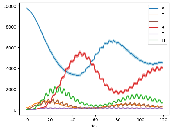
(a) 4 day testing interval, no pooling.

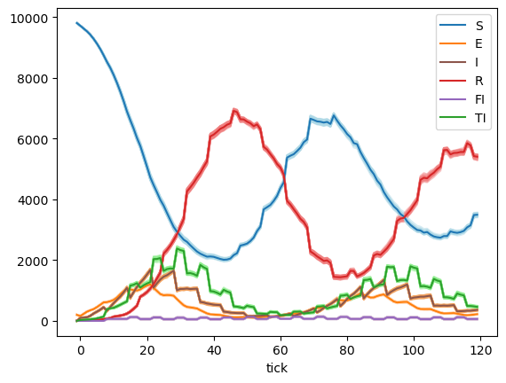
(b) 7 day testing interval, no pooling.

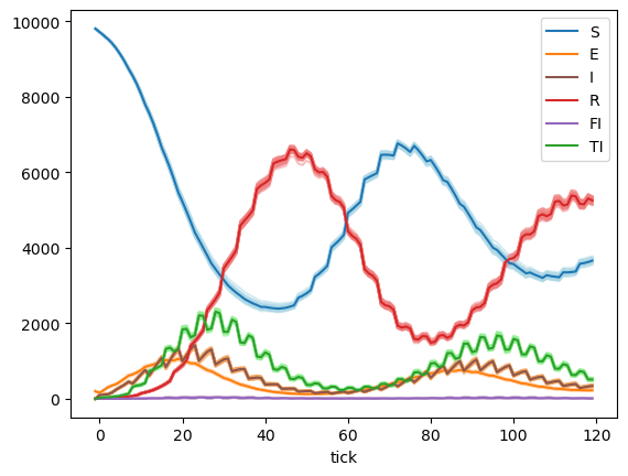
(c) 4 day testing interval, pool size 5.

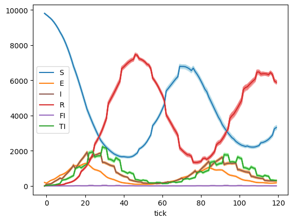
(d) 7 day testing interval, pool size 5.

Figure 3: Vaccination A (no vaccination) + Test B. Subfigures show the number of individuals in the population occupying each of the disease model compartments (susceptible, exposed, infectious, recovered, falsely isolated, and isolated while transmitting). Plots for all 50 runs of each scenario are overlayed on the corresponding subfigure with the average of each compartment over all runs shown in a darker shade.

The most important contribution of our tool is reduced harm to employees. We first demonstrate this in Fig. 3 in a population without vaccination (Vaccination A), while exploring the impact of pooling and/or reduced testing interval. Looking first at the application of test A, we see a decreased number of infections (orange) when testing every 4 days compared to weekly testing. It should be noted that this also comes with an increased cost, although that can be mitigated with pooling of samples (Section 5.3).

For comparison, under the same vaccination status but a faster test return (test B, Fig. 3), we see a similar reduction in the number of infected people between weekly testing scenarios and more frequent testing. In fact, even though test B has a higher rate of false negative, it is more effective at reducing infection (and cost) than test A in most scenarios compared due to its faster turnaround time. The most effective scenarios among test types and testing intervals involve both a faster test turnaround and more frequent testing.

These differences demonstrate that among the options explored, more frequent testing is the most consistent method for reducing disease incidence in a population. Additionally, using a test with faster turn-around can further add to these effects since results are known more quickly for rapid isolation of people who may transmit disease.

5.2 Pooled testing is more effective at reducing false isolation than testing interval

After ensuring the safety of workers, a company’s next concern is loss of productivity, indicated by total people hours lost to infections. Reduced unnecessary isolation also reduces the social impact of a pandemic on a society, improving the mental health of citizens and possibly increasing adherence to testing and quarantine regimes. Therefore, it is not only in a single business’ best interest to reduce false isolation, but there are additional benefits to society outside of work.

Figure 3 (false isolations, ‘PS 1’, ‘4 days’ vs. ‘7 days’), demonstrates the impact of testing interval on false isolation. Paradoxically, longer time between testing reduces the amount of healthy people isolated. This is an artifact of single tests, where the false-positive rate is independent for each test, and thus testing more results in increased false isolation.

In contrast, pooled testing provides a significant reduction in false isolation. Pooling tests reduces the false-positive rate of a pool through our two-stage application - the probability of two false positives is negligible. As such, the minimization of false isolation holds across longer testing regimes (Fig. 3, ‘7 days’) and even with reduced test efficacy (Fig. 3, ‘Test B’).

All of these results are directly compared in Fig. 3. Here, we see the importance of pooled testing, compared to individual testing, under all test efficacy and interval combinations that we explored. Test efficacy is more important than test interval, as test A scenarios generated significant false isolation compared to test B, but this effect is reduced when pooled testing is used. This demonstrates the large reduction in false isolation provided by pooled testing.

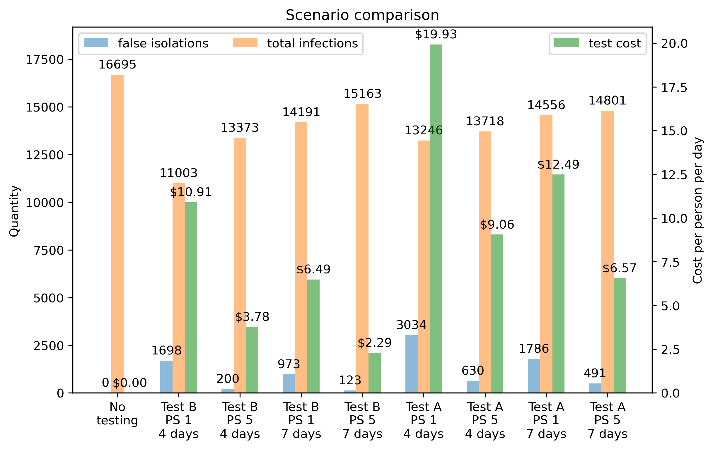
Figure 3: Comparison of testing scenarios in a population with no vaccination (Vaccination A). Scenario labels correspond to the type of test used, pool size (‘PS’) used for pooled testing, and testing interval, respectively. Left and center bars (number of false isolations and total infections) correspond to the y-axis on the left, while the right-most bars (test cost) correspond to the y-axis on the right. Testing scenario cost is based on a cost of $100 for test A and $50 test B. Total testing costs are divided by 120 days and 10,000 people in the population to get the cost per person per day.

5.3 Test cost is effectively reduced under pooling regimes

To be effective, companies must be aware of the bottom line. While ensuring the safety of our employees, it is important to acknowledge the costs of our decisions and, if possible in a safe and effective manner, reduce the expenditure of those actions. Our tool allows direct control over costs by allowing different tests to be provided to simulations. Additionally, a more indirect (but more effective) cost reduction is the application of fewer tests. While this cannot be planned a priori, we can explore which scenarios provide the greatest reduction in test usage as incorporated into reduced overall cost.

Figure 3 shows the total cost per person per day for the tests administered for each scenario. First, we find the obvious conclusion - increasing the testing interval reduces the cost of tests provided. However, we strongly recommend not taking this option, as previous sections have shown reduced testing to increase the incidence of disease in the population and have small benefits for reducing the amount of false isolation.

However, pooled testing also has a significant impact on the total cost of a testing strategy, even more than increasing the testing interval. This option has also been shown to significantly reduce the number of healthy people put into isolation. As such, we believe that pooled testing demonstrates the safest method for reducing the testing burden on a company.

5.4 The impacts of reduced test interval and pooled testing hold across vaccination regimes

We are no longer at the initial stages of the COVID-19 pandemic. At some point, there may be another pandemic, where we need surveillance of a naive population [3]. However, most nations have begun vaccinating their populations and we are now at a state of partial vaccination, with continued vaccine rollout, while we continue surveillance testing. Therefore, we have built our tool to integrate the current levels of employee vaccination within a company, as well as continued vaccination of employees, and we explored the impact of partial vaccination on testing regimes for improved incidence reduction (Table 2). The figures from vaccination scenarios B and C can be found in D.

It should be noted that overall, vaccination of the population does a more effective job at effectively reducing total infection than testing alone (Fig. 3 vs. Figs. 4 and 5). That being said, the results outlined in previous sections hold - the impacts of short versus long intervals between tests on incidence, individual vs pooled testing on false isolation, and across test efficacy. Although the absolute differences in testing regimes appears reduced due to the reduced size of the susceptible population, this does not diminish the trends for reducing infectious cases or false isolation. In fact, it improves the absolute impact of our testing regime, further reducing the amount of infected people or healthy people sent unnecessarily into isolation.

Interestingly, the effect of pooling on test expense is actually increased in a population with higher levels of vaccination. The cost per person associated with single testing increases with the size of the susceptible population, while the cost of pooled testing decreases based on the corresponding lower rate of incidence (test cost, Fig. 3 vs. Figs. 4 and 5). These observations demonstrate the utility of our tool at the early, middle, and through the later stages of a pandemic.

6 Conclusion

The COVID-19 pandemic spurred a need for creation and implementation of testing protocols, quarantine guidelines, and vaccine distribution. Knowledge gleaned from COVID-19 informed the creation of our disease management tool for rapid comparison of infection propagation and response scenarios. While management tools were limited at the beginning of the COVID-19 pandemic, the flexibility of this simulation allows for easy adaptation to different disease scenarios resulting in a shorter start-up time for future epidemics.

The ability to quickly compare the impact of disease interventions is invaluable in management of an epidemic. By integrating infection propagation, agent isolation, testing, and vaccination, this tool can provide non-trivial insights into the relative effectiveness of disease transmission mitigation strategies in a population. This work demonstrated the tool’s utility in the context of COVID-19 management in several populations representing stages of a pandemic. We show that in each of these stages, simulation can be useful for determining the relative effects of management decisions.

In the future, this work could be extended to account for the impact of relationships on disease propagation, with the implementation of social interaction networks [37]. This would provide the ability to simulate the effect of interventions such as varied work schedules. Additionally, we now know that there are several possible outcomes from COVID-19 infection, such as full recovery or partial recovery (“long-term COVID-19”). The model could be expanded to account for different recovery states, as well as death, as this is a more reliable metric for matching simulated outcomes against realized, real-world impacts.

Author contributions statement

K.P., R.V., and J.K. conceived the idea for the simulation tool. K.P. and R.V. developed the code and ran simulations. K.P., J.B., and J.K. assisted in writing the manuscript and preparing for publication.

Additional information

Competing interests

The authors declare no competing interests.

Appendix A Simulation parameters

The full list of parameters for the SICO are listed below by model category. The default values used for the experiments are included in parentheses (excepting those included in Tables 2 and 3). References linking these values to relevant research on the COVID-19 dynamics are included.

A.1 Run parameters

• popSize (10,000): Number of agents in the population

• timeHorizon (120): Length of the simulation in days

• initialInfected (200 or 2% of the population): Number of agents infected at the start of the simulation

• initProportionVaccinated: Proportion of the population initially vaccinated

A.2 Epidemiological model

• betaDaily (0.4): Beta ($\beta$) parameter for daily infection propagation (Eqs. 1 and 2)

• daysTilSusceptible (30): Number of days until an agent becomes susceptible after recovery [38]

• externalExposureProbDaily (0.005): Daily probability ($\gamma$) of being exposed outside of the population

• fractionSymptomatic (0.5): Proportion of infected individuals ($\sigma_{s}$) who develop symptoms [38, 39]

• infectiousViralLoadCut ($10^{3}$): Viral load, $V_{I}$, needed for an agent to become infectious (in cp/ml) [40, 36]

• Viral load model parameters [11]

  • t0 ($\text{uniform}(2.5,3.5)$): Time interval of viral load initialization

  • V0 ($10^{3}$): Initial viral load (cp/ml)

  • tP ($\Gamma(1.5,1)+0.5$): Time interval to achieve peak viral load

  • VP ($\text{uniform}(10^{4},10^{7})$): Peak viral load in cp/ml

  • tS ($\text{uniform}(0,3)$): Time interval for symptoms to begin

  • tF ($\text{uniform}(4,9)$): Time interval for viral load to decline to $V_{F}$ level

  • VF ($10^{3}$): Final viral load level in cp/ml

A.3 Testing

• daysBetweenTesting: Interval at which testing is performed for the population

• daysDelayTestResults: Number of days before a test result is received

• detectionCut: Viral load needed for detection by a test (in cp/ml)

• firstDayOfTesting (7): First day of the simulation to perform testing

• fprSingle: False positive rate for a single test

• fnrSingle: False negative rate for a single test

• poolingType (average): Function to use for computing pooled test results

  • average: Pool detectability is determined by the average of the viral load of all samples in the pool (i.e. a pool is detectable by test $m$ if $\sum_{i=1}^{N}v_{i}/N>l_{m}$, where $v_{i}$ is the viral load of sample $i$, $N$ is the size of the pool, and $l_{m}$ is the limit of detection of test $m$)

  • exponential: Pools are assigned a false positive and false negative testing rate based on the number ($k$) of detectable samples in the pool. The pooling false positive rate is equivalent to that of a single test ($\phi_{p}$), since in either case the viral load is below the detectable threshold. The false negative rate of a pool is equal to the false negative rate of a single test raised to $k$ ($\phi_{n}^{k}$) since each detectable sample contributes to the viral load of the pool and thus decreases the chance of a negative test. In summary, the probability of a pool testing positive is:

    $$p_{+}=\begin{cases}\phi_{p}&k=0\\ 1-\phi_{n}^{k}&k>0\end{cases}.$$

• poolSize: Pool size for test processing (a value of 1 corresponds to no pooled testing)

A.4 Isolation

• noTestingPostIsolationDays (0): Number of days to delay testing of an agent after release from isolation

• isolationLength (10): Number of days an agent is in isolation

• selfIsolationOnSymptomsProb (0.7): Probability that an agent self-isolates when they experience symptoms

A.5 Vaccination

• vaccineAcceptProbMean (0.7): Mean probability that agents are willing to vaccinate

• vaccineAcceptProbStd (0.05): Standard deviation in distribution of probability that agents are willing to vaccinate

• vaccinesAvailablePerDay: Number of vaccines available for distribution during each day of the simulation

• vaccineInfectionProb (0.3): Probability of exposure ($\alpha$) for vaccinated agents (average over the simulation duration based on values in [41])

Appendix B Determining $\beta$

One method for estimating the disease parameters associated with a novel infectious disease is to fit them to the basic reproductive number, $R_{0}$, associated with early stages of an epidemic. For the simulations in this paper, the $\beta$ model parameter representing the average daily number of transmissions made by each infectious agent was estimated using the basic reproductive number estimates associated with COVID-19. $R_{0}$ represents the expected number of exposures resulting from each infectious case in a population where all agents are susceptible. A variety of values for $R_{0}$ have been found for COVID-19 depending on the variant of interest, but generally vary from around 2.5 (ancestral strain) to as high as 7 (Delta strain) or 10 (Omicron strain) [42, 43]. For the experiments in this paper, we aim to simulate an $R_{0}$ around 5, representing a strain that is more transmissible than the ancestral strain but not as transmissible as Omicron or Delta.

The effective reproductive number, $R$, associated with an infectious disease scenario is the actual number of exposures resulting from an infectious agent. This will vary over time based on susceptibility of agents in the population and mitigation strategies employed. The effective reproductive number at the beginning of the epidemic when most agents are susceptible is equivalent to $R_{0}$.

To estimate the $\beta$ parameter, we first create a baseline scenario without intervention (no vaccination or testing). All other parameters (besides $\beta$) are fixed to their values in A. The estimated number of exposure-causing contacts associated with agents internal to the population is given by the second term of Eq. 1 (Eq. 2 can be ignored in this case since $S_{v}=0$). The number of new internal exposures at time step $t$ is then given by

$$E^{\prime}_{i}(t)=\beta\frac{I(t-1)}{P(t-1)}\cdot S_{u}(t-1).$$ (9)

It follows that the average number of exposure causing contacts at time step $t$ per infectious agent is equivalent to $\frac{E^{\prime}_{i}(t)}{I(t-1)}$. The effective reproductive number at time step $t$ can be estimated by

$$R_{t}=\frac{E^{\prime}_{i}(t)}{I(t-1)}\cdot\tau_{I},$$ (10)

where $\tau_{I}$ is the expected amount of time an agent is infectious. Following the model in Section 3.1.2 $\tau_{I}$ can be estimated as,

$$\tau_{I} =\sigma_{s}\;\mathbb{E}\left[t_{0}+t_{P}+t_{S}+t_{F}\right]+(1-\sigma_{s})\;\mathbb{E}\left[t_{0}+t_{P}+t_{F}\right]$$ (11)

$$=\mathbb{E}\left[t_{0}\right]+\mathbb{E}\left[t_{P}\right]+\mathbb{E}\left[t_{F}\right]+\sigma_{s}\;\mathbb{E}\left[t_{S}\right]$$ (12)

$$=3+(1.5+0.5)+6.5+(0.5)(1.5)=12.25.$$ (13)

This uses the fact that $\sigma_{s}=0.5$ and the mean of the Gamma distribution $\Gamma(k,\theta)=k\theta$. Plugging this value into Eq. 10 and simplifying factors gives

$$R_{t}=\frac{\beta S_{u}(t-1)}{P(t-1)}\cdot 12.25.$$ (14)

Assuming $S_{u}(t-1)/P(t-1)\approx 1$ and solving for $R_{t}=5$ gives a $\beta$ value around 0.4. The disease dynamics and effective $R$ value for the baseline scenario with $\beta=0.4$ are given in Fig. 1.

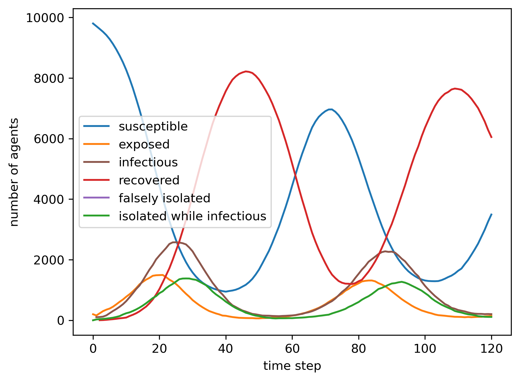
(a) Disease dynamics

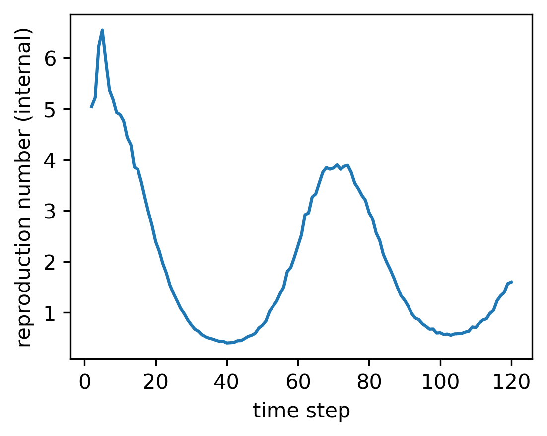
(b) Effective reproductive number

Figure 1: Baseline scenario with $\beta=0.4$.

Appendix C Simulation results: Supplemental figures for vaccination scenario A

(a) 4 day testing interval, no pooling.

(b) 7 day testing interval, no pooling.

Appendix D Simulation results: Vaccination scenarios B and C

For completeness, results of simulations associated with vaccination scenarios B and C (Table 2) are shown here. Figs. 4 and 5 provide comparisons across all scenarios associated with vaccination status B and C, respectively. Scenario labels correspond to the type of test used, pool size used for pooled testing, and testing interval, respectively. Testing scenario cost is based on a cost of $100 for test A and $50 test B. Total testing costs are divided by 120 days and 10,000 people in the population to get the cost per person per day.

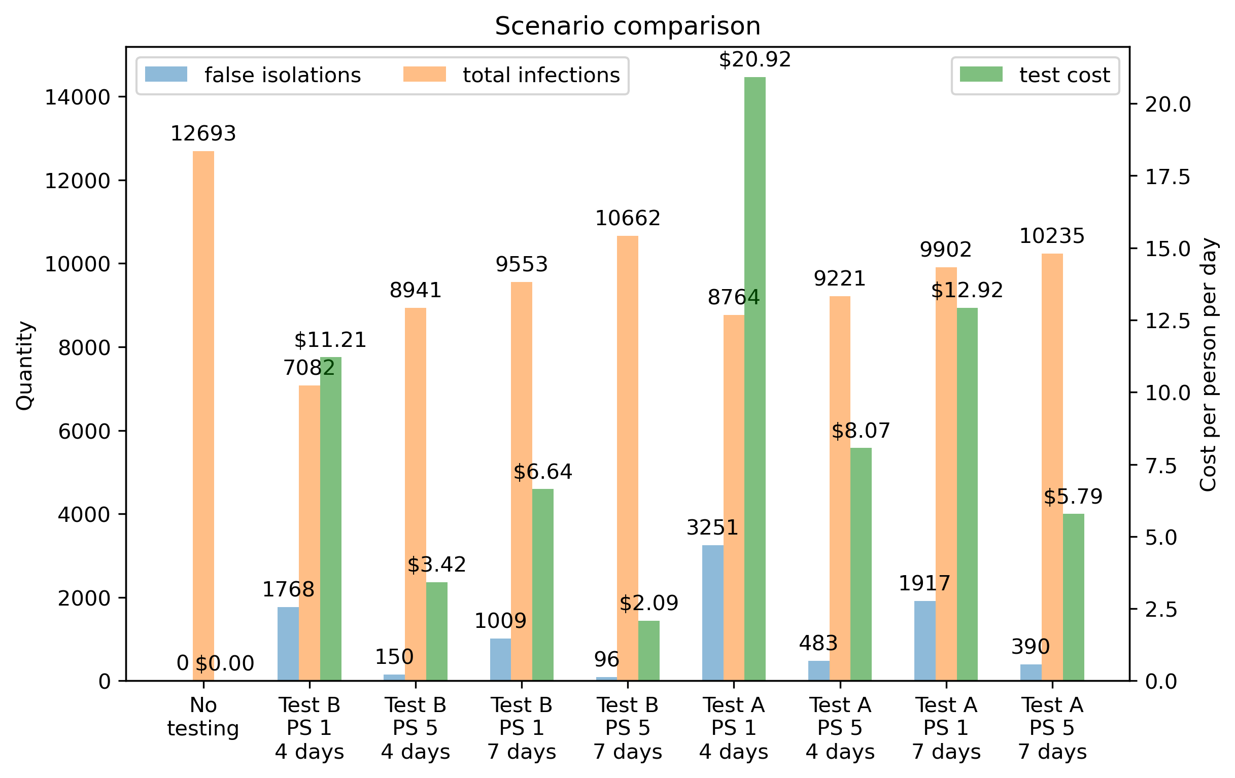
Figure 4: Comparison of testing scenarios in a population with initial vaccine rollout (Vaccination B). Left and center bars (number of false isolations and total infections) correspond to the y-axis on the left, while the right-most bars (test cost) correspond to the y-axis on the right.

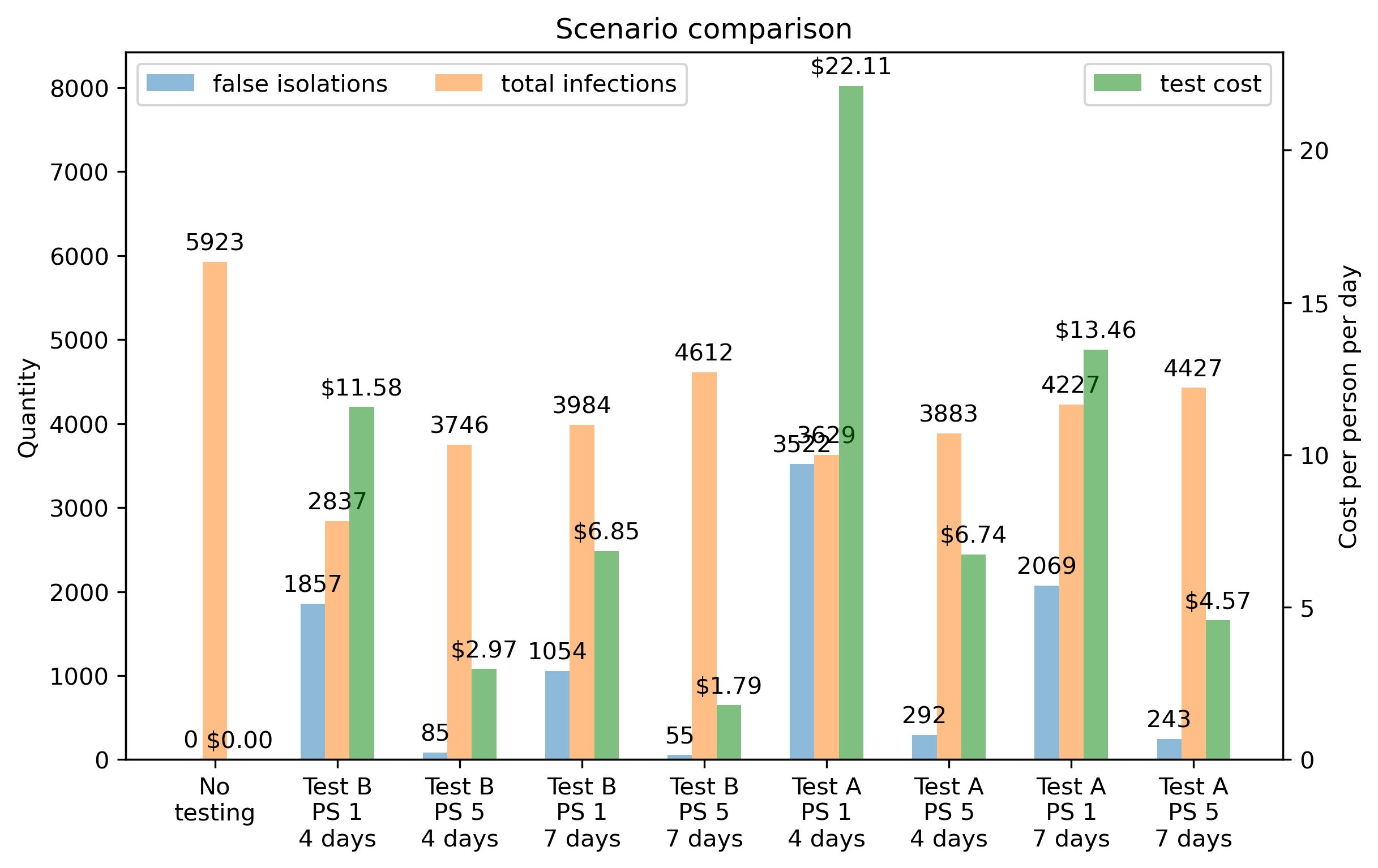
Figure 5: Comparison of testing scenarios in a partially immunized population with continued vaccination rollout (Vaccination C). Left and center bars (number of false isolations and total infections) correspond to the y-axis on the left, while the right-most bars (test cost) correspond to the y-axis on the right.

Appendix E Summary Comparision with the Generalized SEIR Model

In 2020, Liangrong Peng et al. introduced their Generalized SEIR model, which extended the classical SEIR model through the addition of 3 new states [29]. In particular, the Generalized SEIR model partitions a population of size $N$ into the following seven states:

• Susceptible cases

• Insusceptible (i.e. immune or vaccinated) cases

• Exposed, but not yet infectious, cases

• Infectious cases

• Quarantined cases

• Recovered cases

• Closed (i.e. deceased) cases

E. Cheynet added the Generalized SEIR model to the MATLAB code base in 2020 [30], and Felin Wilta et al. utilized Cheynet’s MATLAB implementation of the Generalized SEIR model in their 2022 paper on the death and recovery rates of COVID-19 [44]. SICO extends the functionality of the Generalized SEIR model in a number of noteworthy ways, including:

• The Generalized SEIR model is a dynamical (i.e. ODE) system which models overall trends for a large population. As an ABM, SICO models individual agents’ interactions giving it the flexibility to model a large variety of populations sizes and characteristics.

• SICO is able to separately model the impact of asymptomatic versus symptomatic infectious agents on the spread of an infectious disease.

• In the Generalized SEIR model, Insusceptible cases ($P(t)$) stay insusceptible indefinitely. Whereas instead of having a separate Insusceptible compartment, SICO has two Susceptible states, vaccinated and unvaccinated. Individual susceptible agents in the vaccinated compartment still have a (potentially) non-zero probability of becoming infectious when exposed to the disease. The probability of a vaccinated susceptible agent can be tuned to match a given scenario.

• Similarly, there is no term in the differential equation for $R(t)$ in the Generalized SEIR model to account for loss of immunity by recovered cases. Conversely, SICO is able to model loss of immunity by individual recovered agents.

• SICO can model a variety of disease testing scenarios (including pooled testing), and can model the impact of false negative and false positive tests.

• Under the Generalized SEIR model, only infectious cases can become quarantined cases, and only quarantined cases can become recovered or deceased. In comparison, infectious agents under SICO can become recovered without isolating. Infectious agents who test positive for the disease and healthy agents who receive a false positive for the disease can be moved to isolation. Infectious agents in isolation are moved to the recovered bin after their isolation period is complete, and healthy agents in isolation are moved to one of the two susceptible bins at the end of their isolation period.

• SICO allows a user to specify a stochastic viral load profile for a given disease.

References

- Organization [2023] W. H. Organization, Coronavirus disease (COVID-19), 2023. URL: https://www.who.int/emergencies/diseases/novel-coronavirus-2019. Accessed 27 July 2022.
- Stephanie Oum [2022] J. K. Stephanie Oum, Economic impact of COVID-19 on PEPFAR countries, 2022. URL: https://www.kff.org/global-health-policy/issue-brief/economic-impact-of-covid-19-on-pepfar-countries. Accessed 27 July 2023.
- Marani et al. [2021] M. Marani, G. G. Katul, W. K. Pan, A. J. Parolari, Intensity and frequency of extreme novel epidemics, Proceedings of the National Academy of Sciences 118 (2021) e2105482118. URL: https://www.pnas.org/doi/full/10.1073/pnas.2105482118. Accessed 28 July 2023. doi:10.1073/pnas.2105482118.
- Lyng et al. [2021] G. D. Lyng, N. E. Sheils, C. J. Kennedy, D. O. Griffin, E. M. Berke, Identifying optimal COVID-19 testing strategies for schools and businesses: Balancing testing frequency, individual test technology, and cost, PLOS ONE 16 (2021) e0248783. URL: https://journals.plos.org/plosone/article?id=10.1371/journal.pone.0248783. Accessed 28 July 2023. doi:10.1371/journal.pone.0248783.
- Augenblick et al. [2022] N. Augenblick, J. Kolstad, Z. Obermeyer, A. Wang, Pooled testing efficiency increases with test frequency, Proceedings of the National Academy of Sciences 119 (2022) e2105180119. URL: https://www.pnas.org/doi/abs/10.1073/pnas.2105180119. doi:10.1073/pnas.2105180119.
- Babiker et al. [2020] A. Babiker, C. W. Myers, C. E. Hill, J. Guarner, SARS-CoV-2 Testing: Trials and Tribulations, American Journal of Clinical Pathology 153 (2020) 706–708. URL: https://academic.oup.com/ajcp/article-pdf/153/6/706/33172402/aqaa052.pdf. Accessed 27 July 2023.
- Krause et al. [2021] P. R. Krause, T. R. Fleming, I. M. Longini, R. Peto, S. Briand, D. L. Heymann, V. Beral, M. D. Snape, H. Rees, A.-M. Ropero, R. D. Balicer, J. P. Cramer, C. Muñoz Fontela, M. Gruber, R. Gaspar, J. A. Singh, K. Subbarao, M. D. Van Kerkhove, S. Swaminathan, M. J. Ryan, A.-M. Henao-Restrepo, SARS-CoV-2 Variants and Vaccines, New England Journal of Medicine 385 (2021) 179–186. URL: https://doi.org/10.1056/NEJMsr2105280. Accessed 27 July 2023. doi:10.1056/NEJMsr2105280.
- Guglielmi [2020] G. Guglielmi, The explosion of new coronavirus tests that could help to end the pandemic, 2020. URL: https://www.nature.com/articles/d41586-020-02140-8. Accessed 23 July 2023. doi:10.1038/d41586-020-02140-8.
- Paltiel et al. [2020] A. D. Paltiel, A. Zheng, R. P. Walensky, Assessment of SARS-CoV-2 Screening Strategies to Permit the Safe Reopening of College Campuses in the United States, JAMA Network Open 3 (2020) e2016818. URL: https://doi.org/10.1001/jamanetworkopen.2020.16818. Accessed https://jamanetwork.com/journals/jamanetworkopen/fullarticle/2768923. doi:10.1001/jamanetworkopen.2020.16818.
- Shental et al. [2020] N. Shental, S. Levy, V. Wuvshet, S. Skorniakov, B. Shalem, A. Ottolenghi, Y. Greenshpan, R. Steinberg, A. Edri, R. Gillis, M. Goldhirsh, K. Moscovici, S. Sachren, L. M. Friedman, L. Nesher, Y. Shemer-Avni, A. Porgador, T. Hertz, Efficient high-throughput SARS-CoV-2 testing to detect asymptomatic carriers, Science Advances 6 (2020) eabc5961. URL: https://www.science.org/doi/10.1126/sciadv.abc5961. Accessed 28 July 2023. doi:10.1126/sciadv.abc5961.
- Larremore et al. [2021] D. B. Larremore, B. Wilder, E. Lester, S. Shehata, J. M. Burke, J. A. Hay, M. Tambe, M. J. Mina, R. Parker, Test sensitivity is secondary to frequency and turnaround time for COVID-19 screening, Science Advances 7 (2021). URL: https://www.science.org/doi/10.1126/sciadv.abd5393. Accessed 28 July 2023. doi:10/ghs8s7.
- Nash et al. [2021] B. Nash, A. Badea, A. Reddy, M. Bosch, N. Salcedo, A. R. Gomez, A. Versiani, G. C. D. Silva, T. M. I. L. d. Santos, B. H. G. A. Milhim, M. M. Moraes, G. R. F. Campos, F. Quieroz, A. F. N. Reis, M. L. Nogueira, E. N. Naumova, I. Bosch, B. B. Herrera, Validating and modeling the impact of high-frequency rapid antigen screening on COVID-19 spread and outcomes, 2021. URL: https://www.medrxiv.org/content/10.1101/2020.09.01.20184713v7. Accessed 28 July 2023. doi:10.1101/2020.09.01.20184713.
- Commissioner [2020] O. o. t. Commissioner, Coronavirus (COVID-19) update: FDA informs public about possible accuracy concerns with Abbott ID now point-of-care test, 2020. URL: https://www.fda.gov/news-events/press-announcements/coronavirus-covid-19-update-fda-informs-public-about-possible-accuracy-concerns-abbott-id-now-point. Accessed 27 July 2023.
- Hahn-Klimroth and Müller [2022] M. Hahn-Klimroth, N. Müller, Near optimal efficient decoding from pooled data, 2022. URL: http://arxiv.org/abs/2108.04342. Accessed 23 July 2023. doi:10.48550/arXiv.2108.04342. arXiv:2108.04342.
- Cleary et al. [2021] B. Cleary, J. A. Hay, B. Blumenstiel, M. Harden, M. Cipicchio, J. Bezney, B. Simonton, D. Hong, M. Senghore, A. K. Sesay, S. Gabriel, A. Regev, M. J. Mina, Using viral load and epidemic dynamics to optimize pooled testing in resource-constrained settings, Science Translational Medicine 13 (2021) eabf1568. URL: https://www.science.org/doi/10.1126/scitranslmed.abf1568. Accessed 28 July 2023. doi:10.1126/scitranslmed.abf1568.
- Jonnerby et al. [2020] J. Jonnerby, C. Bronk, D. Sridhar, Test and Contain: A Resource-Optimal Testing Strategy for COVID-19, 2020. URL: https://www.semanticscholar.org/paper/Test-and-Contain%3A-A-Resource-Optimal-Testing-for-Jonnerby-Bronk/0074ba3547f0b23f1d09e01d17ca0e84064d494b.
- sci [2020] Coronavirus antigen tests: Quick and cheap, but too often wrong?, 2020. URL: https://www.science.org/content/article/coronavirus-antigen-tests-quick-and-cheap-too-often-wrong. Accessed 27 July 2023.
- Corman et al. [2020] V. M. Corman, H. F. Rabenau, O. Adams, D. Oberle, M. B. Funk, B. Keller-Stanislawski, J. Timm, C. Drosten, S. Ciesek, SARS-CoV-2 asymptomatic and symptomatic patients and risk for transfusion transmission, Transfusion 60 (2020) 1119–1122. URL: https://onlinelibrary.wiley.com/doi/abs/10.1111/trf.15841. Accessed 28 July 2023. doi:10.1111/trf.15841.
- Asgary et al. [2021] A. Asgary, M. G. Cojocaru, M. M. Najafabadi, J. Wu, Simulating preventative testing of SARS-CoV-2 in schools: policy implications, BMC Public Health 21 (2021) 125. URL: https://bmcpublichealth.biomedcentral.com/articles/10.1186/s12889-020-10153-1. Accessed 28 July 2023. doi:10.1186/s12889-020-10153-1.
- Grassly et al. [2020] N. C. Grassly, M. Pons-Salort, E. P. K. Parker, P. J. White, N. M. Ferguson, K. Ainslie, M. Baguelin, S. Bhatt, A. Boonyasiri, N. Brazeau, L. Cattarino, H. Coupland, Z. Cucunuba, G. Cuomo-Dannenburg, A. Dighe, C. Donnelly, S. L. v. Elsland, R. FitzJohn, S. Flaxman, K. Fraser, K. Gaythorpe, W. Green, A. Hamlet, W. Hinsley, N. Imai, E. Knock, D. Laydon, T. Mellan, S. Mishra, G. Nedjati-Gilani, P. Nouvellet, L. Okell, M. Ragonnet-Cronin, H. A. Thompson, H. J. T. Unwin, M. Vollmer, E. Volz, C. Walters, Y. Wang, O. J. Watson, C. Whittaker, L. Whittles, X. Xi, Comparison of molecular testing strategies for COVID-19 control: a mathematical modelling study, The Lancet Infectious Diseases 20 (2020) 1381–1389. URL: https://www.thelancet.com/journals/laninf/article/PIIS1473-3099(20)30630-7/fulltext. Accessed 28 July 2023. doi:10.1016/S1473-3099(20)30630-7.
- Chin et al. [2020] E. T. Chin, B. Q. Huynh, L. A. C. Chapman, M. Murrill, S. Basu, N. C. Lo, Frequency of Routine Testing for Coronavirus Disease 2019 (COVID-19) in High-risk Healthcare Environments to Reduce Outbreaks, Clinical Infectious Diseases: An Official Publication of the Infectious Diseases Society of America 73 (2020) e3127–e3129. URL: https://www.ncbi.nlm.nih.gov/pmc/articles/PMC7797732/. Accessed 28 July 2023. doi:10.1093/cid/ciaa1383.
- Thi et al. [2020] V. L. D. Thi, K. Herbst, K. Boerner, M. Meurer, L. P. Kremer, D. Kirrmaier, A. Freistaedter, D. Papagiannidis, C. Galmozzi, M. L. Stanifer, S. Boulant, S. Klein, P. Chlanda, D. Khalid, I. B. Miranda, P. Schnitzler, H.-G. Kräusslich, M. Knop, S. Anders, A colorimetric RT-LAMP assay and LAMP-sequencing for detecting SARS-CoV-2 RNA in clinical samples, Science Translational Medicine 12 (2020) eabc7075. URL: https://www.science.org/doi/abs/10.1126/scitranslmed.abc7075. Accessed 28 July 2023. doi:10.1126/scitranslmed.abc7075.
- Butler et al. [2021] D. Butler, C. Mozsary, C. Meydan, J. Foox, J. Rosiene, A. Shaiber, D. Danko, E. Afshinnekoo, M. MacKay, F. J. Sedlazeck, N. A. Ivanov, M. Sierra, D. Pohle, M. Zietz, U. Gisladottir, V. Ramlall, E. T. Sholle, E. J. Schenck, C. D. Westover, C. Hassan, K. Ryon, B. Young, C. Bhattacharya, D. L. Ng, A. C. Granados, Y. A. Santos, V. Servellita, S. Federman, P. Ruggiero, A. Fungtammasan, C.-S. Chin, N. M. Pearson, B. W. Langhorst, N. A. Tanner, Y. Kim, J. W. Reeves, T. D. Hether, S. E. Warren, M. Bailey, J. Gawrys, D. Meleshko, D. Xu, M. Couto-Rodriguez, D. Nagy-Szakal, J. Barrows, H. Wells, N. B. O’Hara, J. A. Rosenfeld, Y. Chen, P. A. D. Steel, A. J. Shemesh, J. Xiang, J. Thierry-Mieg, D. Thierry-Mieg, A. Iftner, D. Bezdan, E. Sanchez, T. R. Campion, J. Sipley, L. Cong, A. Craney, P. Velu, A. M. Melnick, S. Shapira, I. Hajirasouliha, A. Borczuk, T. Iftner, M. Salvatore, M. Loda, L. F. Westblade, M. Cushing, S. Wu, S. Levy, C. Chiu, R. E. Schwartz, N. Tatonetti, H. Rennert, M. Imielinski, C. E. Mason, Shotgun transcriptome, spatial omics, and isothermal profiling of SARS-CoV-2 infection reveals unique host responses, viral diversification, and drug interactions, Nature Communications 12 (2021) 1660. URL: https://www.nature.com/articles/s41467-021-21361-7. Accessed 28 July 2023. doi:10.1038/s41467-021-21361-7.
- Meyerson et al. [2020] N. R. Meyerson, Q. Yang, S. K. Clark, C. L. Paige, W. T. Fattor, A. R. Gilchrist, A. Barbachano-Guerrero, S. L. Sawyer, A community-deployable SARS-CoV-2 screening test using raw saliva with 45 minutes sample-to-results turnaround, medRxiv (2020). URL: https://www.medrxiv.org/content/early/2020/07/17/2020.07.16.20150250. Accessed 28 July 2023. doi:10.1101/2020.07.16.20150250.
- Salcedo et al. [2021] N. Salcedo, A. Harmon, B. B. Herrera, Pooling of Samples for SARS-CoV-2 Detection Using a Rapid Antigen Test, Frontiers in Tropical Diseases 0 (2021). URL: https://www.frontiersin.org/articles/10.3389/fitd.2021.707865/full. Accessed 28 July 2023. doi:10.3389/fitd.2021.707865.
- Aldridge and Ellis [2021] M. Aldridge, D. Ellis, Pooled testing and its applications in the COVID-19 pandemic, 2021. URL: http://arxiv.org/abs/2105.08845. Accessed 28 July 2023. doi:10.48550/arXiv.2105.08845.
- Lock et al. [2022] E. Lock, F. Marmolejo-Cossío, E. Micha, A. D. Procaccia, Welfare-Maximizing Pooled Testing, 2022. URL: http://arxiv.org/abs/2206.10660. Accessed 28 July 2023. doi:10.48550/arXiv.2206.10660. arXiv:2206.10660, arXiv:2206.10660 [cs].
- Dorfman [1943] R. Dorfman, The Detection of Defective Members of Large Populations, The Annals of Mathematical Statistics 14 (1943) 436 – 440. URL: https://doi.org/10.1214/aoms/1177731363. Accessed 28 July 2023. doi:10.1214/aoms/1177731363.
- Peng et al. [2020] L. Peng, W. Yang, D. Zhang, C. Zhuge, L. Hong, Epidemic analysis of COVID-19 in China by dynamical modeling, 2020. arXiv:2002.06563.
- Cheynet [2020] E. Cheynet, Generalized SEIR Epidemic Model (fitting and computation), 2020. URL: https://zenodo.org/record/3911854. Accessed 28 July 2023. doi:10.5281/ZENODO.3911854.
- He et al. [2020] X. He, E. H. Y. Lau, P. Wu, X. Deng, J. Wang, X. Hao, Y. C. Lau, J. Y. Wong, Y. Guan, X. Tan, X. Mo, Y. Chen, B. Liao, W. Chen, F. Hu, Q. Zhang, M. Zhong, Y. Wu, L. Zhao, F. Zhang, B. J. Cowling, F. Li, G. M. Leung, Temporal dynamics in viral shedding and transmissibility of COVID-19, Nature Medicine 26 (2020) 672–675. URL: https://www.nature.com/articles/s41591-020-0869-5. Accessed 28 July 2023. doi:10.1038/s41591-020-0869-5.
- Marc et al. [2021] A. Marc, M. Kerioui, F. Blanquart, J. Bertrand, O. Mitjà, M. Corbacho-Monné, M. Marks, J. Guedj, Quantifying the relationship between SARS-CoV-2 viral load and infectiousness, eLife 10 (2021) e69302. URL: https://elifesciences.org/articles/69302. Accessed 28 July 2023. doi:10.7554/eLife.69302.
- mol [2023] In Vitro Diagnostics EUAs - Molecular Diagnostic Tests for SARS-CoV-2, 2023. URL: https://www.fda.gov/medical-devices/covid-19-emergency-use-authorizations-medical-devices/in-vitro-diagnostics-euas-molecular-diagnostic-tests-sars-cov-2. Accessed 2023-07-05.
- ant [2023] In Vitro Diagnostics EUAs - Antigen Diagnostic Tests for SARS-CoV-2, 2023. URL: https://www.fda.gov/medical-devices/covid-19-emergency-use-authorizations-medical-devices/in-vitro-diagnostics-euas-antigen-diagnostic-tests-sars-cov-2. Accessed 28 July 2023.
- Cubas-Atienzar et al. [2021] A. I. Cubas-Atienzar, K. Kontogianni, T. Edwards, D. Wooding, K. Buist, C. R. Thompson, C. T. Williams, E. I. Patterson, G. L. Hughes, L. Baldwin, C. Escadafal, J. A. Sacks, E. R. Adams, Limit of detection in different matrices of 19 commercially available rapid antigen tests for the detection of SARS-CoV-2, Scientific Reports 11 (2021) 18313. URL: https://www.nature.com/articles/s41598-021-97489-9. Accessed 27 July 2023. doi:10.1038/s41598-021-97489-9.
- Arnaout et al. [2020] R. Arnaout, R. A. Lee, G. R. Lee, C. Callahan, C. F. Yen, K. P. Smith, R. Arora, J. E. Kirby, SARS-CoV2 Testing: The Limit of Detection Matters, preprint, Microbiology, 2020. URL: http://biorxiv.org/lookup/doi/10.1101/2020.06.02.131144. Accessed 28 July 2023. doi:10.1101/2020.06.02.131144.
- Pine et al. [2023] K. Pine, J. Klipfel, J. Bennett, N. Bade, C. Manasseh, Social Network Analysis and Validation of an Agent-Based Model, 2023. arXiv:2308.05256.
- Layton and Sadria [2022] A. T. Layton, M. Sadria, Understanding the dynamics of SARS-CoV-2 variants of concern in Ontario, Canada: a modeling study, Scientific Reports 12 (2022) 2114. URL: https://www.nature.com/articles/s41598-022-06159-x. Accessed 28 July 2023. doi:10.1038/s41598-022-06159-x.
- Ma et al. [2021] Q. Ma, J. Liu, Q. Liu, L. Kang, R. Liu, W. Jing, Y. Wu, M. Liu, Global Percentage of Asymptomatic SARS-CoV-2 Infections Among the Tested Population and Individuals With Confirmed COVID-19 Diagnosis: A Systematic Review and Meta-analysis, JAMA network open 4 (2021) e2137257. URL: https://jamanetwork.com/journals/jamanetworkopen/fullarticle/2787098. Accessed 28 July 2023. doi:10.1001/jamanetworkopen.2021.37257.
- Aspinall [2021] M. G. Aspinall, Viral load and Ct values - How do we use quantitative PCR quantitatively?, 2021. URL: https://chs.asu.edu/diagnostics-commons/blog/how-do-we-use-quantitative-tests-quantitatively. Accessed 28 July 2023.
- hal [2022] Protection against SARS-CoV-2 after Covid-19 Vaccination and Previous Infection, New England Journal of Medicine 386 (2022) 1207–1220. URL: https://www.nejm.org/doi/10.1056/NEJMoa2118691. Accessed 23 July 2023. doi:10.1056/NEJMoa2118691.
- Khandia et al. [2022] R. Khandia, S. Singhal, T. Alqahtani, M. A. Kamal, N. A. El-Shall, F. Nainu, P. A. Desingu, K. Dhama, Emergence of SARS-CoV-2 Omicron (B.1.1.529) variant, salient features, high global health concerns and strategies to counter it amid ongoing COVID-19 pandemic, Environmental Research 209 (2022) 112816. URL: https://www.ncbi.nlm.nih.gov/pmc/articles/PMC8798788/. Accessed 28 July 2023. doi:10.1016/j.envres.2022.112816.
- Burki [2022] T. K. Burki, Omicron variant and booster COVID-19 vaccines, The Lancet. Respiratory Medicine 10 (2022) e17. URL: https://www.ncbi.nlm.nih.gov/pmc/articles/PMC8683118/. Accessed 11 July 2023. doi:10.1016/S2213-2600(21)00559-2.
- Wilta et al. [2022] F. Wilta, A. L. C. Chong, G. Selvachandran, K. Kotecha, W. Ding, Generalized Susceptible-Exposed-Infectious-Recovered model and its contributing factors for analysing the death and recovery rates of the COVID-19 pandemic, Applied Soft Computing 123 (2022) 108973. URL: https://www.sciencedirect.com/science/article/pii/S1568494622003106. Accessed 28 July 2023. doi:10.1016/j.asoc.2022.108973.
Acknowledgements
Work on this research has been funded by the Air Force Research Laboratory (AFRL) Autonomy Capability Team 3 (ACT3) under contracts FA8650-20-C-1121 (K.P., J.K.) and FA8649-20-C-0130 (R.V., J.B.). The authors would like to thank Dr. Michael Mendenhall, Dr. Jared Culbertson, and Dr. Scott Clouse for their assistance.