A finitely convergent circumcenter method for the Convex Feasibility Problem

Abstract

In this paper, we present a variant of the circumcenter method for the Convex Feasibility Problem (CFP), ensuring finite convergence under a Slater assumption. The method replaces exact projections onto the convex sets with projections onto separating halfspaces, perturbed by positive exogenous parameters that decrease to zero along the iterations. If the perturbation parameters decrease slowly enough, such as the terms of a diverging series, finite convergence is achieved. To the best of our knowledge, this is the first circumcenter method for CFP that guarantees finite convergence.

49M27, 65K05, 65B99, 90C25

1 Introduction

The convex feasibility problem (CFP) aims at finding a point in the intersection of $m$ closed and convex sets $C_{i}\subset\mathds{R}^{n}$, $i=1,\ldots,m$, i.e.,

$$\text{find }x^{\star}\in C\coloneqq\bigcap_{i=1}^{m}C_{i}.$$

Convex feasibility represents a modeling paradigm for solving numerous engineering and physics problems, such as image recovery [27], wireless sensor networks localization [33], gene regulatory network inference [45], and many others.

Projection-reflection based methods are widely recognized and effective schemes for solving a diverse range of feasibility problems, including Section 1. These kinds of methods continue to gain popularity due to their ability to strike a balance between high performance and simplicity, as evidenced by their extensive utilization (see, e.g., [11]). Among these methods, two particularly renowned and widely adopted methods are the classical Douglas-Rachford method (DRM) and its modifications (see, e.g., [8, 32, 2]), and the famous method of alternating projections (MAP) (see, e.g., [10, 9]). The elementary Euclidean concept of circumcenter has recently been employed to improve the convergence of those classical projection-reflection methods for solving the CFP (1). The circumcentered-reflection method (CRM) was first presented in [20] as an acceleration technique for DRM for the two set affine CFP. Since then, CRM has been shown as a valid and powerful new tool for solving (non)convex structured feasibility problems because of its ability to minimize the inherent zig-zag behavior of projection-reflection based methods, in particular. In [22], for instance, CRM was connected to the classical MAP. Moreover, CRM obviates the spiraling behavior for the classical DRM [30, 37, 29]. as an acceleration technique for DRM for the two set affine CFP. Since then, CRM has been shown as a valid and powerful new tool for solving (non)convex structured feasibility problems because of its ability to minimize the inherent zig-zag behavior of projection-reflection based methods. In [22], for instance, CRM was connected to the classical MAP. Moreover, CRM was used to obviate the spiraling behavior of the classical DRM [30, 37, 29]. CRM was further studied in [4, 6, 7, 22, 24, 17, 19, 18, 12, 13, 14, 15, 16, 38, 42, 39, 40, 41, 3, 5].

The circumcenter of three points $x,y,z\in\mathds{R}^{n}$, denoted as $\operatorname{circ}(x,y,z)$, is the point in $\mathds{R}^{n}$ that lies in the affine manifold spanned by $x,y$ and $z$ and is equidistant to these three points. Given two closed convex sets $A,B\subset\mathds{R}^{n}$, the CRM iterates by means of the operator ${\mathscr{C}}_{A,B}:\mathds{R}^{n}\to\mathds{R}^{n}$ defined as

$${\mathscr{C}}_{A,B}(x)\coloneqq\operatorname{circ}(x,R_{A}(x),R_{B}(R_{A}(x)),$$

where $P_{A}:\mathds{R}^{n}\to A,P_{B}:\mathds{R}^{n}\to B$ are the orthogonal projections onto $A,B$ respectively, $R_{A}=2P_{A}-\operatorname{Id}$, $R_{B}=2P_{B}-\operatorname{Id}$ (i.e., $R_{A},R_{B}$ are the reflections onto $A$, $B$, respectively), and $\operatorname{Id}$ is the identity operator in $\mathds{R}^{n}$. Hence, the sequence generated by CRM is defined as

$$x^{k+1}={\mathscr{C}}_{A,B}(x^{k}).$$

If $x^{k}\in A\cap B$, then the sequence stops at iteration $k$, in which case, we say that the algorithm has finite convergence.

One limitation of CRM is that its convergence theory requires one of the sets to be an affine manifold. In [20], it was pointed out that the iteration defined in Section 1 may fail to be well-defined or to approach $A\cap B$. Subsequently, a specific counterexample was presented in [1] where CRM does not converge for two general convex sets. However, CRM can be used to solve the general CFP with $m$ general arbitrary closed convex sets by employing Pierra’s product space reformulation, as presented in [43].

Define $\mathbf{C}\coloneqq C_{1}\times\cdots\times C_{m}\subset\mathds{R}^{nm}$ and $\mathbf{D}\coloneqq\{(x,x,\ldots,x)\in\mathds{R}^{nm}\mid x\in\mathds{R}^{n}\}$. $\mathbf{D}$ is said to be the diagonal subspace in $\mathds{R}^{nm}$. One can easily see that

$$x^{\star}\in C\Leftrightarrow\mathbf{z}^{\star}\coloneqq(x^{\star},x^{\star},\ldots,x^{\star})\in\mathbf{C}\cap\mathbf{D}.$$

Due to Section 1, solving Section 1 corresponds to solving

$$\text{find }\mathbf{z}^{\star}\in\mathbf{C}\cap\mathbf{D}.$$

Since $\mathbf{D}$ is an affine manifold, CRM can be applied to finding a point in $\mathbf{C}\cap\mathbf{D}$ in the product space $\mathds{R}^{nm}$.

In [6], it was proven that the Circumcenter Reflected Method (CRM) with Pierra’s product space reformulation achieves a superior convergence rate compared to the Method of Alternating Projections (MAP) [10, 9]. The iteration operator of MAP is simply the composition of alternating projections, $P_{A}\circ P_{B}$. Furthermore, in the same paper, it was shown that for certain special cases, circumcenter schemes such as CRM attain a superlinear rate of convergence [6, 18], and even linear convergence in the absence of an error bound. Notably, no other known method utilizing individual projections achieves such complexity even for these particular cases.

More recently, an extension of CRM, called cCRM (acronym for centralized circumcentered-reflection method), was introduced in [19] to overcome the drawback of CRM, namely the requirement that one of the sets be an affine manifold. The cCRM can solve the CFP for any pair of closed and convex sets and converges linearly under an error-bound condition (similar to a transversality hypothesis), and superlinearly if the boundaries of the convex sets are smooth. Still, for solving the CFP with $m$ sets, it is necessary to go through the Pierra reformulation in the product space.

To solve the CFP with $m$ sets more efficiently, a successive extension of cCRM, called ScCRM, was developed in [17]. ScCRM avoids the product space reformulation and inherits from cCRM the linear and superlinear convergence rates under the error-bound and smoothness hypothesis, respectively.

All the aforementioned methods require several exact orthogonal projections onto some of the convex sets in each iteration. However, determining the exact orthogonal projection is computationally expensive in practice, except in some very special cases. This limitation was overcome in [4], where an approximate version of CRM, called CARM, is proposed. CARM replaces the exact projections onto the original sets with projections onto sets containing them (e.g., halfspaces or Cartesian products of halfspaces), which are easily computable.

In this paper, we improve upon the aforementioned methods by introducing an algorithm in the product space that uses projections onto perturbed halfspaces, referred to as PACA (Perturbed Approximate Circumcenter Algorithm). PACA’s iteration reads as follows

$$\mathbf{x}^{k+1}={\mathscr{C}}_{\mathbf{S}^{k},\mathbf{D}}(\mathbf{x}^{k})=\operatorname{circ}(\mathbf{x}^{k},R_{\mathbf{S}^{k}}(\mathbf{x}^{k}),R_{\mathbf{D}}(R_{\mathbf{S}^{k}}(\mathbf{x}^{k}))).$$

For any $\mathbf{x}^{0}\in\mathbf{D}$, we will be able to obtain a circumcenter sequence in $\mathbf{D}$ generated by means of Section 1 converging in finitely many steps to a point in $\mathbf{C}\cap\mathbf{D}$, if the Slater condition holds. This is possible by strategically building the perturbed halfspaces $\mathbf{S}^{k}$ (see Sections 3 and 4).

The paper is organized as follows: In Section 2, we present some definitions and preliminary material. In Section 3, we state our algorithm, PACA, Section 4, shows the development of the convergence analysis. Finally, Section 5 shows the linear convergence rate of the sequence generated by our algorithm. Finite convergence is proved in Section 6 under additional assumptions on the perturbation parameters. Finally, Section 7 presents numerical experiments to solve ellipsoids intersection comparing PACA with CARM (in the product space), the Simultaneous (Cimmino [26]) subgradient projection method (SSPM) by [34], and the Modified Cyclic (Kaczmarz [35]) subgradient projection method (CSPM) from [28].

2 Preliminary results

In this paper, we consider the CFP as in Section 1, assuming that the sets $C_{i}$ are given as:

$$C_{i}=\{x\in\mathds{R}^{n}\mid f_{i}(x)\leq 0\}$$

where $f_{i}:\mathds{R}^{n}\rightarrow\mathds{R}$ is a convex function for $i=1,\ldots,m$.

This formulation does not impose any limitations in principle, as we can always choose $f_{i}(x)=\left\|P_{C_{i}}(x)-x\right\|$. However, this choice is not consistent with the later imposition of the Slater hypothesis. Nevertheless, in most instances of the CFP, it is possible to formulate them as in Section 2 using suitable functions $f_{i}$.

A basic assumption for our finite convergence result is the Slater condition, defined as follows:

Definition 2.1 (Slater condition).

There exists $\hat{x}\in\mathds{R}^{n}$ such that

$$f_{i}(\hat{x})<0,$$

for all $i=1,\ldots,m$.

We continue by recalling the explicit formula of the orthogonal projection onto a halfspace.

Proposition 2.2.

If $H=\{y\in\mathds{R}^{n}\mid a^{\top}y\leq\alpha\}$, with $a\in\mathds{R}^{n}$, $\alpha\in R$, then the orthogonal projection onto $H$ is given by

$$P_{H}(x)=x-\frac{\max\{0,\alpha-a^{\top}x\}}{\|a\|^{2}}a.$$

Proof 2.3.

The result follows from the definition of orthogonal projection after an elementary calculation.

The following proposition is a key result concerning the circumcenter operator ${\mathscr{C}}_{A,B}$, as defined in Section 1. It represents the only result pertaining to circumcenter steps that will be used in our convergence analysis.

Proposition 2.4.

Let $A$ and $B$ be closed convex subsets of $\mathds{R}^{n}$. Consider the circumcenter operator ${\mathscr{C}}_{A,B}$ defined in Section 1. Suppose that $B$ is an affine manifold. Then, for all $x\in B$ there exists a closed and convex set $H(x)\subset\mathds{R}^{n}$ such that, for all $x\in\mathds{R}^{n}$,

1. $A\subset H(x)$;

2. ${\mathscr{C}}_{A,B}(x)=P_{H(x)\cap B}(x)$;

3. ${\mathscr{C}}_{A,B}(x)$ belongs to $B$;

4. $\left\lVert{\mathscr{C}}_{A,B}(x)-s\right\rVert^{2}\leq\left\lVert x-s\right\rVert^{2}-\left\lVert{\mathscr{C}}_{A,B}(x)-x\right\rVert^{2}$ for all $s\in A$.

Proof 2.5.

The result follows from Lemma 3 in [20]; cf. also Lemma 3.3 and Lemma 3.4 in [4]. In fact $H(x)$ is a halfspace containing $A$, with an explicit formula, which ensures that item (i) holds, but this is irrelevant for our purposes. We also mention that item (ii) is the essential result, while items (iii) and (iv) follow immediately from it.

A useful concept for analyzing the convergence of projection-based algorithms is the notion of Fejér monotonicity. A sequence $\{y^{k}\}\subset\mathds{R}^{n}$ is said to be Fejér monotone with respect to a set $M\subset\mathds{R}^{n}$ if $\lVert y^{k+1}-y\rVert\leq\lVert y^{k}-y\rVert$ for all $y\in M$ and all $k\in\mathbb{N}$. It is known that if $\{y^{k}\}$ is Fejér monotone with respect to $M$, then $\{y^{k}\}$ is bounded, and if it has a cluster point $y^{\star}\in M$, then the entire sequence $\{y^{k}\}$ converges to $y^{\star}$. In our analysis, we require a slightly weaker notion and also need to handle cases where $M$ is open, and the cluster points of $\{y^{k}\}$ belong to the boundary of $M$. We now introduce the appropriate tools to address this situation.

Definition 2.6 (Fejér* monotonicity).

Let $M\subset\mathds{R}^{n}$ and consider a sequence $\{y^{k}\}\subset\mathds{R}^{n}$. We say that $\{y^{k}\}$ is Fejér* monotone with respect to $M$ if for any point $y\in M$, there exists $N(y)\in\mathds{N}$ such that

$$\left\lVert y^{k+1}-y\right\rVert\leq\left\lVert y^{k}-y\right\rVert$$

for all $k\geq N(y)$.

Note that the difference with the usual Fejér monotonicity notion lies in the fact that now the decreasing distance property holds for the tail of the sequence, starting at some index which depends on the point $s$. Next we present the extension of the Fejér monotonicity results needed for our analysis. We recall first the notions of R-linear and Q-linear convergence. A sequence $\{y^{k}\}\subset\mathds{R}^{n}$ converges Q-linearly to $y^{\star}\in\mathds{R}^{n}$ if

$$\limsup_{k\to\infty}\frac{\left\lVert y_{k+1}-y^{\star}\right\rVert}{\left\lVert y^{k}-y^{\star}\right\rVert}=\eta<1,$$

and R-linearly if

$$\limsup_{k\to\infty}\left\lVert y^{k}-y^{\star}\right\rVert^{1/k}=\eta<1.$$

The value $\eta$ is said to be the asymptotic constant. It is well known that Q-linear convergence implies R-linear convergence with the same asymptotic constant.

Theorem 2.7 (Characterization of Fejér* monotonicity).

Suppose that $M\subset\mathds{R}^{n}$ is a closed and convex set with nonempty interior and $\{y^{k}\}\subset\mathds{R}^{n}$ is Fejér* monotone with respect to $\operatorname{int}(M)$ (the interior of $M$). Then,

1. the sequence $\{y^{k}\}$ is bounded;

2. if there exists a cluster point $\bar{y}$ of $\{y^{k}\}$ which belongs to $M$, then the whole sequence $\{y^{k}\}$ converges to $\bar{y}$;

3. if $\{y^{k}\}$ converges to $y^{\star}\in M$ and $\{\operatorname{dist}(y^{k},M)\}$ converges Q- or R-linearly to $0$ with asymptotic constant $\eta$, then $\{y^{k}\}$ converges R-linearly to $y^{\star}$ with the same asymptotic constant.

Proof 2.8.

To prove (i), take any point $y\in M$. From the definition of Fejér* monotonicity, we conclude that $y^{k}$ belongs to the ball with center at $y$ and radius $\left\lVert y^{N(y)}-y\right\rVert$ for all $k\geq N(y)$. Consequently, $\{y^{k}\}$ is bounded.

The item (ii) follows after let $\bar{y}\in M$ be a cluster point of $\{y^{k}\}$ and $\{y^{\ell_{k}}\}$ be a subsequence of $\{y^{k}\}$ such that $\lim_{k\to\infty}y^{\ell_{k}}=\bar{y}\in M$. Take any $\hat{y}\in\operatorname{int}(M)$. Since $M$ is convex and $\bar{y}\in M$, the whole open segment between $\hat{y}$ and $\bar{y}$ is contained in $\operatorname{int}(M)$. Given any $\gamma>0$, take now any $y$ in such open segment such that $\left\lVert y-\bar{y}\right\rVert\leq\frac{\gamma}{4}$. Since $\{y^{k}\}$ is Fejér* monotone to $\operatorname{int}(M)$, there exists $N(y)$ such that for all $k\geq N(y)$, we have

$$\left\lVert y^{k+1}-y\right\rVert\leq\left\lVert y^{k}-y\right\rVert.$$

Take $K\in\mathds{N}$ such that $\ell_{K}\geq N(y)$ and $\left\lVert y^{\ell_{K}}-\bar{y}\right\rVert\leq\frac{\gamma}{4}$. Hence, we get from 2.8

$$\left\lVert y^{k}-y\right\rVert\leq\left\lVert y^{\ell_{K}}-y\right\rVert\leq\left\lVert y^{\ell_{K}}-\bar{y}\right\rVert+\left\lVert\bar{y}-y\right\rVert\leq\frac{\gamma}{4}+\frac{\gamma}{4}\leq\frac{\gamma}{2},$$

for all $k\geq\ell_{K}$. Therefore, in view of 2.8,

$$\left\lVert y^{k}-\bar{y}\right\rVert\leq\left\lVert y^{k}-y\right\rVert+\left\lVert y-\bar{y}\right\rVert\leq\frac{\gamma}{2}+\frac{\gamma}{4}\leq\gamma$$

for all $k\geq\ell_{K}$. Since $\gamma$ is an arbitrary positive number, we conclude that $\bar{y}=\lim_{k\to\infty}y^{k}$.

For proving (iii) note again that Fejér* monotonicity of $\{y^{k}\}$ implies that for each $\hat{y}\in\operatorname{int}(M)$ there exists $N(\hat{y})$ such that $\left\lVert y^{k+m}-\hat{y}\right\rVert\leq\left\lVert y^{k}-\hat{y}\right\rVert$ for all $k\geq N(\hat{y})$ and all $m\in\mathds{N}$. Hence,

$$\|y^{k+m}-y^{k}\|\leq\|y^{k+m}-\hat{y}\|+\|y^{k}-\hat{y}\|\leq 2\|y^{k}-\hat{y}\|,$$

for all $\hat{y}\in\operatorname{int}(M)$, all $k\geq N(\hat{y})$ and all $m\in\mathds{N}$. Taking limits in 2.8 with $m\to\infty$, we get

$$\left\lVert y^{k}-y^{\star}\right\rVert\leq 2\left\lVert y^{k}-\hat{y}\right\rVert$$

for all $\hat{y}\in\operatorname{int}(M)$. Let $z^{k}=P_{M}(y^{k})$, so that $z^{k}\in M$. As in item (ii), convexity of $M$ ensures the existence of $\hat{y}\in\operatorname{int}(M)$ such that $\left\lVert\hat{y}-z^{k}\right\rVert\leq\left\lVert y^{k}-z^{k}\right\rVert$. Hence, in view of 2.8,

(1) $$\left\lVert y^{k}-y^{\star}\right\rVert \leq 2\left\lVert y^{k}-\hat{y}\right\rVert\leq 2\left\lVert y^{k}-\hat{y}\right\rVert$$

(2) $$\leq 2\left\lVert y^{k}-z^{k}\right\rVert+2\left\lVert\hat{y}-z^{k}\right\rVert$$

(3) $$\leq 2\left\lVert y^{k}-z^{k}\right\rVert+2\left\lVert y^{k}-z^{k}\right\rVert$$

(4) $$=4\left\lVert y^{k}-z^{k}\right\rVert=4\,\operatorname{dist}(y^{k},M).$$

Taking $k$-th roots in both sides of the last inequality, we get

$$\left\lVert y^{k}-y^{\star}\right\rVert^{1/k}\leq 4^{1/k}\operatorname{dist}(y^{k},M)^{1/k}.$$

In view of the relation between Q-linear and R-linear convergence,

$$\limsup_{k\to\infty}\left\lVert y^{k}-y^{\star}\right\rVert^{1/k}\leq\limsup_{k\to\infty}\operatorname{dist}(y^{k},M)^{1/k}=\eta<1.$$

3 Statement of the algorithm

We are now ready to introduce the Perturbed Approximate Circumcenter Algorithm (PACA) for the CFP defined in Section 2. Let us assume that the sets $C_{i}$, $i=1,\ldots,m$ in the CFP Section 1 take the form described in Section 2. Given an arbitrary initial point $x^{0}\in\mathds{R}^{n}$ and a decreasing sequence of perturbation parameters $\{\epsilon_{k}\}$ which converges to $0$, the PACA scheme for solving CFP is defined as follows:

• Initialization.

  Take $x^{0}\in\mathds{R}^{n}$.

• Iterative step.

  Given $x^{k}$, take $u^{ik}\in\partial f_{i}(x^{k})$, the subdifferential of $f_{i}$ at $x^{k}$ (so, $u^{ik}$ is a subgradient of $f_{i}$ at $x^{k}$), and define:

  $$v^{ik}\coloneqq\left[\frac{\max\{0,f_{i}(x^{k})+\epsilon_{k}\}}{\left\lVert u^{ik}\right\rVert^{2}}\right]u^{ik},$$

  $$w^{k}\coloneqq\frac{1}{m}\sum_{i=1}^{m}v^{ik}.$$

  If $w^{k}=0$, then take $x^{k+1}=x^{k}$ and proceed to the $(k+1)$-th iteration. Otherwise, define

  $$\alpha_{k}\coloneqq\frac{\frac{1}{m}\sum_{i=1}^{m}\left\lVert v^{ik}\right\rVert^{2}}{\left\lVert w^{k}\right\rVert^{2}},$$

  $$x^{k+1}\coloneqq x^{k}-\alpha_{k}w^{k}.$$

• Stopping criterion.

  If $x^{k}\in C\coloneqq\cap_{i=1}^{m}C_{i}$, then stop (in this case, we say that PACA has finite convergence).

We now provide a somewhat informal explanation of several properties of the sequence $\{x^{k}\}$ genarating by PACA. By examining 2) with $\epsilon_{k}=0$, and considering Proposition 2.2, it becomes evident that $x^{k}-v^{ik}$ represents the orthogonal projection of $x^{k}$ onto a halfspace containing $C_{i}$, while $x^{k}-w^{k}$ is a convex combination of such projections. With the presence of perturbation parameters $\epsilon_{k}$, $x^{k}-v^{ik}$ corresponds to the projection of $x^{k}$ onto the perturbed set $S^{k}_{i}$, defined as:

$$S_{i}^{k}=\begin{dcases*}C_{i}^{k},&if $x^{k}\in C_{i}^{k}$,\\ \{z\in\mathds{R}^{n}\mid(u^{i})^{\top}(z-x^{k})+f_{i}(x^{k})+\epsilon_{k}\leq 0\},&otherwise,\end{dcases*}$$

which contains the perturbed convex set

$$C_{i}^{k}\coloneqq\{x\in\mathds{R}^{n}\mid f_{i}(x)+\epsilon_{k}\leq 0\},$$

as we will prove in Proposition 4.1. We mention that, depending on the value of $\epsilon_{k}$, the set $C^{k}_{i}$ may be empty. On the other hand, $S^{k}_{i}$ is always nonempty, so that the sequence $\{x^{k}\}$ is always well-defined, independently of the value of $\epsilon_{k}$. However, the set $S^{k}\coloneqq\cap_{i=1}^{m}S^{k}_{i}$ may still be empty, in which case the sequence $\{x^{k}\}$ may exhibit an erratic behavior. It could even happen that $w^{k}=0$, in which case, as stated in the Iterative Step, we get $x^{k+1}=x^{k}$. This only occurs if, by chance, $x^{k}$ minimizes the function $\sum_{i=1}^{m}\left\lVert x-P_{S^{k}_{i}}(x)\right\rVert^{2}$. In this case the sequence does not stop: it proceeds to the next iteration, with perturbation parameter $\epsilon_{k+1}<\epsilon_{k}$. For large enough $k$, however, the set $S^{k}$ will become nonempty; this is ensured to happen when the Slater point $\hat{x}$ gets inside $S^{k}$ (more precisely, when $k$ is large enough so that $\epsilon_{k}<\min_{1\leq i\leq m}\{\left\lvert f_{i}(\hat{x})\right\rvert\}$). At that point, the sequence starts moving toward $S^{k}$, and a fortiori toward $C^{k}\coloneqq\cap_{i=1}^{m}C^{k}_{i}\subset S^{k}$, so that eventually it converges to a point in $C$.

We also observe that $x^{k}-w^{k}$ is a convex combination, with equal weights, of the projections onto the perturbed sets $S^{k}_{i}$. The factor $\alpha_{k}$ in the definition of $x^{k+1}$ (i.e., in 2)) encapsulates the contribution of the circumcentered-reflection approach, as we will discuss in the next section.

It is easy to verify that if $\epsilon_{k}=0$ for all $k$, then the PACA sequence coincides with the CARM sequence in [4], using the separating operator given in Example 2.7 of [4]. If we remove the factor $\alpha_{k}$ in 2), PACA reduces to Algorithm 4 in [34] with relaxation parameters equal to $1$. In this case, $x^{k+1}$ is simply a convex combination of perturbed approximate projections of $x^{k}$ onto the sets $C_{i}$. We mention that this algorithm also enjoys finite convergence, under the same assumptions as in Theorem 6.3 in this paper.

Proposition 3.1.

Consider the PACA sequence defined by 2), 2), 2), and 2). Then, $\alpha_{k}\geq 1$ for all $k$.

Proof 3.2.

The result follows directly from 2) and 2), and the convexity of the function $\left\lVert\cdot\right\rVert^{2}$.

Proposition 3.1 indicates that the PACA sequence can be seen as an overrelaxed version of the sequence given by $x^{k+1}=x^{k}-w^{k}$, studied in [34]. We comment that the particular value of $\alpha_{k}$ determined in 2), related to the circumcenter approach, has special consequences in terms of the performance of the method.

4 Convergence Analysis

For the convergence analysis, it is necessary to establish a connection between PACA and the CRM method applied to a CFP in the product space $\mathds{R}^{nm}$. This allows us to utilize Pierra’s formulation, which transforms a CFP with $m$ sets in $\mathds{R}^{n}$ into a CFP with only two sets in $\mathds{R}^{nm}$, with one of them being a linear subspace.

Consider $C^{k}_{i}$ as defined in Section 3 (once again, we recall that $C^{k}_{i}$ may be empty for some values of $\epsilon_{k}$) and $S_{i}^{k}$, as defined in Section 3. Using Proposition 2.2, the projection of $x^{k}$ onto $S_{i}^{k}$ is given by:

$$P_{S_{i}^{k}}(x^{k})=x^{k}-\frac{\max\{0,f_{i}(x^{k})+\epsilon_{k}\}}{\|u^{ik}\|^{2}}u^{ik},$$

with $u^{ik}\in\partial f_{i}(x^{k})$. i.e., $u^{ik}$ is a subgradient of $f_{i}$ at $x^{k}$. We remark that Section 4 also works when $x^{k}$ belongs to $C^{k}_{i}$, in which case $S_{i}^{k}$ is not a halfspace, but just the set $C^{i}_{k}$, and $P_{S_{i}^{k}}(x^{k})=x^{k}$.

Now we introduce the appropriate sets in $\mathds{R}^{nm}$ for using Pierra’s formulation. Define:

$$\mathbf{S}^{k}=S_{1}^{k}\times\dots\times S_{m}^{k},$$

and

$$\mathbf{C}^{k}=C_{1}^{k}\times\dots\times C_{m}^{k}.$$

We need an elementary result on the relation between $\mathbf{C}^{k}$ and $\mathbf{S}^{k}$.

Proposition 4.1.

Take $\mathbf{S}^{k},\mathbf{C}^{k}\subset\mathds{R}^{nm}$ as defined in Sections 4 and 4, respectively. Then,

$$\mathbf{C}^{k}\subset\mathbf{S}^{k}.$$

Proof 4.2.

The result holds trivially if $\mathbf{C}^{k}$ is empty (i.e., if $C_{i}^{k}=\emptyset$ for some $i$). Otherwise, it suffices to prove that $C_{i}^{k}\subset S_{i}^{k}$ for all $i$. Take any point $z\in C_{i}^{k}$, so that $f_{i}(z)+\epsilon_{k}\leq 0$. If $x^{k}\in C_{i}^{k}$, then the result is satisfied by the definition of $S_{i}^{k}$. If $x^{k}\notin S_{i}^{k}$, since the $f_{i}$’s are convex, then we have

$$(u^{ik})^{\top}(z-x^{k})+f_{i}(x^{k})+\epsilon_{k}\leq f_{i}(z)+\epsilon^{k}\leq 0,$$

for all $z\in\mathds{R}^{n}$, using Section 3 and the definition of subgradient. The result follows from 4.2 and the definition of $S^{k}_{i}$ (i.e., Section 3), since $z\in S_{i}^{k}$ for all $i$.

Recall that $\mathbf{D}\subset\mathds{R}^{nm}$ is the diagonal subspace in $\mathds{R}^{nm}$. In the next lemma, we will prove that the sequence $\{\mathbf{x}^{k}\}\subset\mathds{R}^{nm}$ generated by CRM with the sets $\mathbf{S}^{k}$ and $\mathbf{D}$ is related to the sequence $\{x^{k}\}\subset\mathds{R}^{n}$ generated by PACA with the sets $C^{k}_{i}$. In fact, we will get that $\mathbf{x}^{k}=(x^{k},x^{k},\dots,x^{k})$ for all $k$.

Lemma 4.3.

Assume that $C_{i}\subset\mathds{R}^{n}$ is in the form of Section 2 and $f_{i}:\mathds{R}^{n}\to\mathds{R}$ is convex for all $i$. Consider the set $\mathbf{S}^{k}$ as defined in Section 3 and the sequence $\{\mathbf{x}^{k}\}\subset\mathds{R}^{nm}$ generated by CRM starting from $\mathbf{x}^{0}\in\mathds{R}^{nm}$ using the sets $\mathbf{S}^{k}$ and ${\mathbf{D}}$ at iteration $k$ as given in Section 1, i.e.,

$$\mathbf{x}^{k+1}\coloneqq{\mathscr{C}}_{\mathbf{S}^{k},\mathbf{D}}(\mathbf{x}^{k})=\operatorname{circ}(\mathbf{x}^{k},R_{\mathbf{S}^{k}}(\mathbf{x}^{k}),R_{\mathbf{D}}(R_{\mathbf{S}^{k}}(\mathbf{x}^{k}))),$$

where $R_{\mathbf{S}^{k}}\coloneqq 2P_{\mathbf{S}^{k}}-\operatorname{Id}$, $R_{\mathbf{D}}\coloneqq 2P_{\mathbf{D}}-\operatorname{Id}$. Let $\{x^{k}\}\subset\mathds{R}^{n}$ be generated by PACA as in 2) starting from $x^{0}\in\mathds{R}^{n}$. If $\mathbf{x}^{0}=(x^{0},\ldots,x^{0})$, then $\mathbf{x}^{k}=(x^{k},\ldots,x^{k})$ for all $k\geq 1$. Also, PACA stops at iteration $k$ iff CRM does so.

Proof 4.4.

Since $\mathbf{x}^{0}\in\mathbf{D}$, and $\mathbf{D}$ is an affine subspace, we get that $\mathbf{x}^{k}\in\mathbf{D}$ by Proposition 2.4(ii), for all $k\geq 0$. Therefore, we suppose that $\mathbf{x}^{k}=(y^{k},\ldots,y^{k})$ with $y^{k}\in\mathds{R}^{n}$. Since $\mathbf{x}^{0}=(x^{0},\dots,x^{0})$, we assume inductively that $y^{k}=x^{k}$, and we must prove that $\mathbf{x}^{k+1}=(x^{k+1},\dots,x^{k+1})$. We proceed to compute the arguments of the right-hand side of Lemma 4.3 in order to get ${\mathscr{C}}_{\mathbf{S}^{k},\mathbf{D}}(\mathbf{x}^{k})$. By Section 4, we get

$$P_{\mathbf{S}^{k}}(\mathbf{x}^{k})=\left(P_{S^{k}_{1}}(x^{k}),\dots,P_{S^{k}_{m}}(x^{k})\right).$$

Moreover, Section 4 and 2) yields

$$P_{S_{i}^{k}}(x^{k})=x^{k}-\frac{\max\{0,f_{i}(x^{k})+\epsilon_{k}\}}{\left\lVert u^{ik}\right\rVert^{2}}u^{ik}=x^{k}-v^{ik},$$

with $u^{ik}\in\partial f_{i}(x^{k})$. It follows from 4.4 and 4.4 that

$$P_{\mathbf{S}^{k}}(\mathbf{x}^{k})=\left(x^{k}-v^{1k},\dots,x^{k}-v^{mk}\right).$$

In view of 4.4 and of the definition of the reflection operator, we have

$$R_{\mathbf{S}^{k}}(\mathbf{x}^{k})=\left(x^{k}-2v^{1k},\dots,x^{k}-2v^{mk}\right).$$

It follows from the definition of the diagonal subspace $\mathbf{D}$ that $P_{\mathbf{D}}(x^{1},\dots,x^{m})=(z,\dots,z)$ with $z=(1/m)\sum_{i=1}^{m}x^{i}$. Hence, in view of 2),

$$P_{\mathbf{D}}(\mathbf{x}^{k})=(x^{k}-2w^{k},\dots,x^{k}-2w^{k}).$$

Finally, in view of 4.4,

$$R_{\mathbf{D}}\left(R_{\mathbf{S}^{k}}(\mathbf{x}^{k})\right)=(x^{k}-4w^{k},\dots,x^{k}-4w^{k}).$$

Now, by the definition of circumcenters, ${\mathscr{C}}_{\mathbf{S}^{k},\mathbf{D}}(\mathbf{x}^{k})$ must be equidistant to $\mathbf{x},\mathbf{y}$ and $\mathbf{z}$, with $\mathbf{y}\coloneqq R_{\mathbf{S}^{k}}(\mathbf{x})$ as in 4.4 and $\mathbf{z}\coloneqq R_{\mathbf{D}}\left(R_{\bf S^{k}}(\mathbf{x}^{k})\right)$ as in 4.4. An elementary but somewhat lengthy calculation using 4.4 and 4.4 shows that any vector of the form ${\bf e}(\alpha)=(x^{k}-\alpha w^{k},\dots,x^{k}-\alpha w^{k})$ with $\alpha\in\mathds{R}$ is equidistant from $\mathbf{y}$ and $\mathbf{z}$.

Note that the equation $\left\lVert{\bf e}(\alpha)-\mathbf{x}\right\rVert^{2}=\left\lVert{\bf e}(\alpha)-\mathbf{z}\right\rVert^{2}$, leads, after some elementary calculations, to a linear equation in $\alpha$, whose solution is $\alpha=\alpha_{k}$, with $\alpha_{k}$ as in 2). Hence, taking into account 2), we get

$$\mathbf{x}^{k+1}={\mathscr{C}}_{\mathbf{S}^{k},\mathbf{D}}(\mathbf{x}^{k})=(x^{k}-\alpha_{k}w^{k},\dots,x^{k}-\alpha_{k}w^{k})=(x^{k+1},\dots,x^{k+1}),$$

completing the inductive step. The equivalence between the stopping criteria of both algorithms is immediate.

Another useful result is the quasi-nonexpansiveness of the CRM operator ${\mathscr{C}}_{\mathbf{S}^{k},\mathbf{D}}$, with respect to $\mathbf{C}^{k}$.

Lemma 4.5 (Quasi-nonexpansiveness of ${\mathscr{C}}_{\mathbf{S}^{k},\mathbf{D}}$).

Let $\mathbf{S}^{k},\mathbf{C}^{k}\subset\mathds{R}^{nm}$ be defined as in Sections 4 and 4, respectively. Consider the operator ${\mathscr{C}}_{\mathbf{S}^{k},\mathbf{D}}$ as defined in Section 1 and assume that $\mathbf{C}^{k}\neq\emptyset$. Then,

$$\left\lVert{\mathscr{C}}_{\mathbf{S}^{k},\mathbf{D}}(\mathbf{x})-{\bf s}\right\rVert^{2}\leq\left\lVert\mathbf{x}-{\bf s}\right\rVert^{2}-\left\lVert{\mathscr{C}}_{\mathbf{S}^{k},\mathbf{D}}(\mathbf{x})-\mathbf{x}\right\rVert^{2}$$

for all $\mathbf{x}\in\mathds{R}^{nm}$ and all ${\bf s}\in\mathbf{C}^{k}$.

Proof 4.6.

Since $S_{i}^{k}$ is closed and convex by definition, then $\mathbf{S}^{k}$ is also closed and convex. The result follows immediately from Proposition 2.4(iii) and Proposition 4.1, with $\mathbf{S}^{k}$ playing the role of $A$ and $\mathbf{D}$, the role of $B$.

Next, we prove that the sequence generated by PACA is Fejér* monotone with respect to $\operatorname{int}(C)$.

Lemma 4.7.

Consider CFP with the $C^{i}$’s of the form Section 2. Suppose that $\{x^{k}\}\subset\mathds{R}^{n}$ is the sequence generated by PACA starting at $x^{0}\in R^{n}$. If the sequence $\{x^{k}\}$ is infinite, then,

1. $\{x^{k}\}$ is Fejér* monotone with respect to $\operatorname{int}(C)$;

2. $\lim_{k\to\infty}\left\lVert x^{k+1}-x^{k}\right\rVert=0$;

3. The sequence $\{x^{k}\}$ is bounded.

Proof 4.8.

For item (i), let $\{\mathbf{x}^{k}\}\subset\mathds{R}^{nm}$ be the sequence generated by CRM as in Lemma 4.3 starting at $\mathbf{x}^{0}=(x^{0},\ldots,x^{0})$. By definition of $\mathbf{x}^{0}$, it belongs to $\mathbf{D}\subset\mathds{R}^{nm}$. By Proposition 2.4(ii) and Lemma 4.3, $\mathbf{x}^{k}\in\mathbf{D}$ for all $k$. Define

$$C^{k}\coloneqq\bigcap_{i=1}^{m}C_{i}^{k}.$$

From Lemma 4.5 and Lemma 4.3, we get

$$\left\lVert\mathbf{x}^{k+1}-{\bf s}\right\rVert^{2}\leq\left\lVert\mathbf{x}^{k}-{\bf s}\right\rVert^{2}-\left\lVert\mathbf{x}^{k+1}-\mathbf{x}^{k}\right\rVert^{2},$$

for all ${\bf s}\in\mathbf{C}^{k}\cap\mathbf{D}$. Since $\{\mathbf{x}^{k}\}\subset\mathbf{D}$ and ${\bf s}\in\mathbf{D}$, we have, in view of Lemma 4.3, $\mathbf{x}^{k}=(x^{k},\dots,x^{k})$, $\mathbf{x}^{k+1}=(x^{k+1},\dots,x^{k+1})$ and ${\bf s}=(s,\dots,s)$ with $s\in C^{k}\subset\mathds{R}^{n}$ as defined in 4.8, so that $\left\lVert\mathbf{x}^{k+1}-{\bf s}\right\rVert^{2}=m\left\lVert x^{k+1}-s\right\rVert^{2}$, $\left\lVert\mathbf{x}^{k}-{\bf s}\right\rVert^{2}=m\left\lVert x^{k}-s\right\rVert^{2}$ and $\left\lVert\mathbf{x}^{k+1}-\mathbf{x}^{k}\right\rVert^{2}=m\left\lVert x^{k+1}-x^{k}\right\rVert^{2}$. Hence, it follows from 4.8 that

$$\left\lVert x^{k+1}-s\right\rVert^{2}\leq\left\lVert x^{k}-s\right\rVert^{2}-\left\lVert x^{k+1}-x^{k}\right\rVert^{2},$$

for all $s\in C^{k}$ as defined in 4.8. The Slater condition implies that $\operatorname{int}(C)\neq\emptyset$. Take any $s\in\operatorname{int}(C)$, so that $f_{i}(s)<0$ for all $i$. Since $\{\epsilon_{k}\}$ converges to $0$, there exists $N(s)\in\mathds{N}$, such that $\epsilon_{k}<\min_{1\leq i\leq m}\left\lvert f_{i}(s)\right\rvert$ for all $k>N(s)$. Therefore, we have $s\in\mathbf{C}^{k}$ for all $k>N(s)$. Hence, in view of 4.8

$$\left\lVert x^{k+1}-s\right\rVert^{2}\leq\left\lVert x^{k}-s\right\rVert^{2},$$

for all $s\in\operatorname{int}(C)$ and all $k\geq N(s)$. In view of the definition of Fejér* monotonicity, $\{x^{k}\}$ is Fejér* monotone with respect to $\operatorname{int}(C)$.

To prove (ii) note that 4.8 implies that $\left\{\left\lVert x^{k}-s\right\rVert\right\}$ is decreasing and nonnegative. Hence, $\left\{\left\lVert x^{k}-s\right\rVert\right\}$ is convergent, and also

$$\left\lVert x^{k+1}-x^{k}\right\rVert^{2}\leq\left\lVert x^{k}-s\right\rVert^{2}-\left\lVert x^{k+1}-s\right\rVert^{2},$$

which immediately implies the result.

For item (iii) notice that the Slater condition implies that $\operatorname{int}(C)\neq\emptyset$. Then the result follows from item (i) and Theorem 2.7(i).

Next we prove that the cluster points of the sequence generated by PACA solve the CFP Section 1.

Proposition 4.9.

Let $\{x^{k}\}$ be the sequence generated by PACA. If $\{x^{k}\}$ is infinite and $\bar{x}$ is a cluster point of $\{x^{k}\}$, then $\bar{x}\in C$.

Proof 4.10.

First, note that the existence of cluster points of $\{x^{k}\}$ follows from Lemma 4.7. Let $\hat{x}$ be a Slater point for the CFP. Since all the $f_{i}$’s are convex and $f_{i}(\hat{x})<0$ for all $i$, we get from the definition of subgradient that

$$(u^{ik})^{\top}(\hat{x}-x^{k})\leq f_{i}(\hat{x})-f_{i}(x^{k})\leq-f_{i}(x^{k}),$$

Let $\{x^{\ell_{k}}\}$ be a subsequence of $\{x^{k}\}$ which converges to the cluster point $\bar{x}$. By 2),

$$x^{k}-x^{k+1}=\alpha_{k}w^{k}.$$

Multiplying both sides of 4.10 by $\hat{x}-x^{k}$, we get

(5) $$(x^{k}-x^{k+1})^{\top}(\hat{x}-x^{k}) =\alpha_{k}(w^{k})^{\top}(\hat{x}-x^{k})$$

(6) $$=\frac{\alpha_{k}}{m}\sum_{i=1}^{m}\frac{\max\{0,f_{i}(x^{k})+\epsilon_{k}\}}{\|u^{ik}\|^{2}}(u^{ik})^{\top}(\hat{x}-x^{k})$$

(7) $$\leq-\frac{\alpha_{k}}{m}\sum_{i=1}^{m}\frac{\max\{0,f_{i}(x^{l_{k}})+\epsilon_{k}\}}{\|u^{ik}\|^{2}}f_{i}(x^{k}),$$

where the inequality holds by 4.10. Rearranging the last inequality, we get

(8) $$(x^{k+1}-x^{k})^{\top}(\hat{x}-x^{k}) \geq\frac{\alpha_{k}}{m}\sum_{i=1}^{m}\frac{\max\{0,f_{i}(x^{k})+\epsilon_{k}\}}{\|u^{ik}\|^{2}}f_{i}(x^{k})$$

(9) $$\geq\frac{1}{m}\sum_{i=1}^{m}\frac{\max\{0,f_{i}(x^{k})+\epsilon_{k}\}}{\|u^{ik}\|^{2}},$$

using Proposition 3.1. Since $\{x^{k}\}$ is bounded by Theorem 2.7(i) and the subdifferential is locally bounded (see. e.g., Theorem 3 in [44]), we refine the subsequence $\{x^{\ell_{k}}\},$ if needed, in order to ensure that for each $i$, $\{u^{i\ell_{k}}\}$ converges, say to $\bar{u}^{i}$. Let $I\coloneqq\{i:f_{i}(\bar{x})\geq 0\}$. We take limits with $k\to\infty$ on both sides of Eq. 9 along the refined subsequence $\{x^{\ell_{k}}\}$, getting

(10) $$0\geq\frac{1}{m}\sum_{1\leq i\leq m}\frac{\max\{0,f_{i}(\bar{x})\}f_{i}(\bar{x})}{\left\lVert\bar{u}^{i}\right\rVert^{2}}=\frac{1}{m}\sum_{i\in I}\left(\frac{f_{i}(\bar{x})}{\left\lVert\bar{u}^{i}\right\rVert}\right)^{2}$$

because $\lim_{k\to\infty}\epsilon_{k}=0$ and $\lim_{k\to\infty}(x^{k+1}-x^{k})=0$ by Lemma 4.7(ii). It follows from (10) that $f_{i}(\bar{x})=0$ for all $i\in I$. Since, by the definition of $I$, $f_{i}(\bar{x})<0$ for all $i\notin I$, we get that $f_{i}(\bar{x})\leq 0$ for $i=1,\ldots,m$. Therefore, we conclude that $\bar{x}\in C$.

We close this section by establishing convergence of the full sequence generated by PACA to a solution of the CFP Section 1.

Theorem 4.11.

Let $\{x^{k}\}$ be the sequence generated by PACA starting from an arbitrary point $x^{0}\in\mathds{R}^{n}$. If $\{x^{k}\}$ is infinite, then it converges to some $x^{\star}\in C$.

Proof 4.12.

By Lemma 4.7(iii), $\{x^{k}\}$ is bounded, so that it has cluster points. Proposition 4.9 yields that its cluster points belong to $C$. Finally, Theorem 2.7(ii) implies that $\{x^{k}\}$ converges to some $x^{\star}\in C$.

5 Linear convergence rate

In this section we will prove that if the sequence generated by PACA is infinite, then under the Slater condition it enjoys a linear convergence rate. It is worth mentioning that in other papers addressing circumcentered-reflection methods, such as [18, 6, 21, 4], a linear rate of the generated sequence was proved under an error bound (or transversality) assumption [36, 23]. This assumption is somewhat weaker than our Slater condition (see Proposition 3.2, Theorem 3.3 and the last paragraph of Subsection 3.1 in [18]) but under the Slater condition we can achieve a better result, namely finite convergence. In the above-mentioned references the asymptotic constant related to the linear convergence depends on some constants linked to the error bound assumption; as it could be expected, our asymptotic constant is given in terms of the Slater point.

Proposition 5.1.

Let $\{x^{k}\}$ be the sequence generated by PACA. If $\{x^{k}\}$ is infinite, then there exist $N\in\mathds{N}$ such that

$$\operatorname{dist}^{2}(x^{k+1},C^{k})\leq\operatorname{dist}^{2}(x^{k},C^{k})-\left\lVert x^{k+1}-x^{k}\right\rVert^{2},$$

for all $k>N$

Proof 5.2.

We have proved in 4.8 that

$$\left\lVert x^{k+1}-s\right\rVert^{2}\leq\left\lVert x^{k}-s\right\rVert^{2}-\left\lVert x^{k+1}-x^{k}\right\rVert^{2},$$

and all $k>N$ and all $s\in C^{k}$. The result follows by taking minimum with $s\in C^{k}$ in both sides of 5.2.

Proposition 5.3.

Let $\{x^{k}\}$ be the sequence generated by PACA. If $\{x^{k}\}$ is infinite, then there exist $N\in\mathds{N}$, $\beta\in\mathds{R}$ and an index $\ell(k)\in\{1,\ldots,m\}$ such that

$$\operatorname{dist}^{2}(x^{k},C^{k})\leq\beta^{2}(f_{\ell(k)}(x^{k})+\epsilon_{k})^{2},$$

for all $k\geq N$.

Proof 5.4.

Let $\hat{x}$ be a Slater point. Define:

$$I_{k}\coloneqq\{i\mid f_{i}(x^{k})+\epsilon_{k}>0\},$$

$$\gamma_{i}^{k}\coloneqq 1-\frac{f_{i}(x^{k})+\epsilon_{k}}{f_{i}(x^{k})-f_{i}(\hat{x})}=-\frac{f_{i}(\hat{x})+\epsilon_{k}}{f_{i}(x^{k})-f_{i}(\hat{x})},$$

$$\ell(k)\coloneqq\operatorname*{arg\,min}_{i\in I_{k}}\{\gamma_{i}^{k}\},$$

$$y^{ik}\coloneqq(1-\gamma_{i}^{k})\hat{x}+\gamma_{i}^{k}x^{k},$$

$$\gamma^{k}\coloneqq\gamma_{\ell(k)}^{k}$$

and

$$y^{k}\coloneqq(1-\gamma^{k})\hat{x}+\gamma^{k}x^{k}.$$

First, we claim that for large enough $k$ and $i\in I_{k}$, we have $0<\gamma_{i}^{k}<1$. Define

$$\xi\coloneqq\frac{1}{2}\min_{1\leq i\leq m}\left\lvert f_{i}(\hat{x})\right\rvert,$$

and take $N\in\mathds{N}$ such that

$$\epsilon_{k}\leq\xi$$

for all $k\geq N$. It follows from 5.4 and 5.4 that $\hat{x}\in C^{k}$. Then, $f_{i}(\hat{x})+\epsilon_{k}\leq 0$ for all $i$. Therefore

$$f_{i}(x^{k})-f_{i}(\hat{x})\geq f_{i}(x^{k})+\epsilon_{k}>0.$$

Observe that, for $i\in I_{k}$, $0<\gamma_{k}<1$. We claim that $y^{k}$ belongs to $C^{k}=\cap_{i=1}^{m}C_{i}^{k}$. By convexity of $f_{i}$, 5.4, and 5.4, for $i\in I_{k}$,

$$f_{i}(y^{ik})\leq(1-\gamma_{i}^{k})f_{i}(\hat{x})+\gamma_{i}^{k}f_{i}(x^{k})=-\epsilon_{k}.$$

So $y^{ik}\in C_{i}^{k}$. By convexity of $C^{k}_{i}$, if $\mu\leq\gamma_{i}^{k}$, the point $y(\mu)=(1-\mu)\hat{x}+\mu x^{k}$ also belongs to $C^{k}_{i}$. It follows that if

$$\mu\leq\gamma^{k}_{i}$$

for all $i\in I_{k}$, then $y(\mu)$ belongs to $C^{k}_{i}$ for all $i\in I_{k}$. By 5.4 and 5.4, $\mu=\gamma^{k}=\gamma_{\ell(k)}^{k}$ satisfies 5.4 and so, in view of 5.4, $y^{k}=y(\mu)\in C^{k}_{i}$ for all $i\in I_{k}$.

For $i\notin I_{k}$, both $x^{k}$ and $\hat{x}$ belong to $C_{i}^{k}$ and $y^{k}$ is in the segment between them. It follows that $y^{k}\in C_{i}^{k}$ for $i\in\{1,\ldots,m\}$ and the claim is established. Hence,

(11) $$\operatorname{dist}^{2}(x^{k},C^{k}) \leq\left\lVert x^{k}-y^{k}\right\rVert^{2}=(1-\gamma_{k})^{2}\|x^{k}-\hat{x}\|^{2}$$

(12) $$=(f_{\ell(k)}(x^{k})+\epsilon_{k})^{2}\frac{\|x^{k}-\hat{x}\|^{2}}{(f_{\ell(k)}(x^{k})-f_{\ell(k)}(\hat{x}))^{2}}.$$

Now we look for an appropriate lower bound for the denominator in the rightmost expression in Eq. 12, namely $(f_{\ell(k)}(x^{k})-f_{\ell(k)}(\hat{x}))^{2}$. Since $\ell(k)\in I_{k}$ by 5.4, we have that $f_{\ell(k)}(x^{k})\geq\epsilon_{k}$, so that

$$f_{\ell(k)}(x^{k})-f_{\ell(k)}(\hat{x})\geq-\epsilon_{k}-f_{\ell(k)}(\hat{x})=-\epsilon_{k}+\left\lvert f_{\ell(k)}(\hat{x})\right\rvert\geq-\epsilon_{k}+2\xi\geq-\xi+2\xi=\xi,$$

using the fact that $f_{\ell(k)}(\hat{x})<0$ in the first equality, 5.4 in the second inequality and 5.4 in the third one. It follows from 5.4 that $(f_{\ell(k)}(x^{k})-f_{\ell(k)}(\hat{x}))^{2}\geq\xi^{2}$ and hence, in view of 5.4

$$\operatorname{dist}^{2}(x^{k},C^{k})\leq(f_{\ell(k)}(x^{k})+\epsilon_{k})^{2}\frac{\|x^{k}-\hat{x}\|^{2}}{\xi^{2}}.$$

Since $\{x^{k}\}$ is bounded there exists $\theta>0$ such that $\left\lVert x^{k}-\hat{x}\right\rVert\leq\theta$ for all $k$, so that 5.4 implies

$$\operatorname{dist}^{2}(x^{k},C^{k})\leq\beta^{2}(f_{\ell(k)}(x^{k})+\epsilon_{k})^{2},$$

with $\beta=\theta/\xi$.

Proposition 5.5.

Let $\{x^{k}\}$ be the sequence generated by PACA, starting from $x^{0}\in\mathds{R}^{n}$. If $\{x^{k}\}$ is infinite, then there exists $N\in\mathds{N}$ and $\sigma>0$ such that

$$\operatorname{dist}^{2}(x^{k},C^{k})\leq m(\beta\sigma)^{2}\left\lVert x^{k+1}-x^{k}\right\rVert^{2},$$

for all $k\geq N$.

Proof 5.6.

Since $\{x^{k}\}$ is bounded, and the subdifferential of a convex function defined on the whole $\mathds{R}^{n}$ is locally bounded (see, e.g., Theorem 3 in [44]), we can take $\sigma\in\mathds{R}$ such that

$$\left\lVert u^{ik}\right\rVert\leq\sigma$$

for all $k$ and all $i$. If needed, we also take $\sigma$ large enough so that $m(\beta\sigma)^{2}>1$.

Let $\{\mathbf{x}^{k}\}\subset\mathds{R}^{nm}$ be the sequence generated by CRM as in Lemma 4.3 starting at $\mathbf{x}^{0}=(x^{0},\ldots,x^{0})$. Then,

(13) $$2\left\lVert\mathbf{x}^{k}-P_{\mathbf{S}^{k}}(\mathbf{x}^{k})\right\rVert =\left\lVert\mathbf{x}^{k}-R_{\mathbf{S}^{k}}(\mathbf{x}^{k})\right\rVert\leq\left\lVert\mathbf{x}^{k}-\mathbf{x}^{k+1}\right\rVert+\left\lVert\mathbf{x}^{k+1}-R_{\bf S^{k}}(\mathbf{x}^{k})\right\rVert$$

(14) $$=2\left\lVert\mathbf{x}^{k+1}-\mathbf{x}^{k}\right\rVert,$$

using the definition of reflection in the first equality, and the definition of circumcenter, together with Section 1 and Section 1, in the second one. It follows from Eq. 14 that

$$\left\lVert\mathbf{x}^{k+1}-\mathbf{x}^{k}\right\rVert^{2}\geq\left\lVert\mathbf{x}^{k}-P_{\mathbf{S}^{k}}(\mathbf{x}^{k})\right\rVert^{2}.$$

In view of Lemma 4.3, we pass from $\mathds{R}^{nm}$ to $\mathds{R}^{n}$ in 5.6, obtaining

$$m\left\lVert x^{x+1}-x^{k}\right\rVert^{2}\geq\sum_{i=1}^{m}\left\lVert x^{k}-P_{S_{i}^{k}}(x^{k})\right\rVert^{2}=\sum_{i=1}^{m}\left\lVert\frac{\max\{0,f_{i}(x^{k})+\epsilon_{k}\}}{\|u^{ik}\|^{2}}u^{ik}\right\rVert^{2}$$

$$=\sum_{i=1}^{m}\left[\frac{\max\{0,f_{i}(x^{k})+\epsilon_{k}\}}{\left\lVert u^{ik}\right\rVert}\right]^{2}=\sum_{i\in I_{k}}\left[\frac{f_{i}(x^{k})+\epsilon_{k}}{\left\lVert u^{ik}\right\rVert}\right]^{2}\geq\left[\frac{f_{\ell(k)}+\epsilon_{k}}{\sigma}\right]^{2},$$

with $I_{k}$ and $\ell(k)$ as defined in 5.4 and 5.4 respectively. The first equality in 5.6 holds by Section 4, the third equality by 5.4, and the second inequality follows from 5.4 ($\ell(k)$ belongs to $I_{k}$), and 5.6.

Take $N$ as in Proposition 5.3. Combining 5.6 with Proposition 5.3, we obtain

$$\operatorname{dist}^{2}(x^{k},C^{k})\leq\beta^{2}(f_{\ell(k)}(x^{k})+\epsilon_{k})^{2}\leq m(\beta\sigma)^{2}\left\lVert x^{k+1}-x^{k}\right\rVert^{2}$$

for all $k>N$, completing the proof.

Proposition 5.7.

Let $\{x^{k}\}$ be the sequence generated by PACA. If $\{x^{k}\}$ is infinite, then the sequence $\{\operatorname{dist}(x^{k},C^{k})\}$ converges Q-linearly to $0$.

Proof 5.8.

By Proposition 5.1, there exists $N\in\mathds{N}$ such that

$$\operatorname{dist}^{2}(x^{k+1},C^{k})\leq\operatorname{dist}^{2}(x^{k},C^{k})-\left\lVert x^{k+1}-x^{k}\right\rVert^{2}$$

for all $k\geq N$. Since $\{\epsilon_{k}\}$ is monotonically decreasing, we have $C^{k}\subset C^{k+1}$, so that we get from 5.8,

$$\operatorname{dist}^{2}(x^{k+1},C^{k+1})\leq\operatorname{dist}^{2}(x^{k},C^{k})-\left\lVert x^{k+1}-x^{k}\right\rVert^{2}.$$

Using Proposition 5.5 and 5.8, we get

$$\operatorname{dist}(x^{k+1},C^{k+1})\leq\sqrt{1-\frac{1}{m(\beta\sigma)^{2}}}\,\operatorname{dist}(x^{k},C^{k}),$$

completing the proof.

Next we prove that the sequence $\{\operatorname{dist}(x^{k},C)\}$ converges R-linearly to $0$.

Proposition 5.9.

Let $\{x^{k}\}$ be the sequence generated by PACA. If $\{x^{k}\}$ is infinite, then the sequence $\{dist(x^{k},C)\}$ converges R-linearly to $0$.

Proof 5.10.

Let

$$\lambda=\sqrt{1-\frac{1}{m(\beta\sigma)^{2}}}$$

with $\beta,\sigma$ as in Proposition 5.7. By Proposition 5.7, there exists $N\in\mathds{N}$ such that, for $k>N$,

$$\operatorname{dist}(x^{k},C^{k})\leq\lambda^{k-1-N}\operatorname{dist}(x^{N},C^{N}).$$

Since $C^{k}\subset C$ for all $k$, we get from 5.10,

$$\operatorname{dist}(x^{k},C)\leq\operatorname{dist}(x^{k},C^{k})\leq\lambda^{k-1-N}\operatorname{dist}(x^{N},C^{N})$$

for all $k\geq N$. Taking $k$-th roots in 5.10 and then limits with $k\to\infty$, we get

$$\lim_{k\to\infty}[\operatorname{dist}(x^{k},C)]^{1/k}=\lim_{k\to\infty}\lambda^{1-(N+1)/k}[\operatorname{dist}(x^{N},C^{N})]^{1/k}=\lambda.$$

Since $\lambda<1$ by 5.10, we conclude that $\{\operatorname{dist}(x^{k},C)\}$ converges R-linearly to $0$.

Theorem 5.11.

Let $\{x^{k}\}$ be the sequence generated by PACA starting from an arbitrary point $x^{0}\in\mathds{R}^{n}$. If $\{x^{k}\}$ is infinite, then $\{x^{k}\}$ converges R-linearly to some point $x^{\star}\in C$.

Proof 5.12.

The result is a direct consequence of Proposition 5.9 and Theorem 2.7(iii).

6 Finite Convergence

In this section we will prove that under an additional assumption on the sequence of perturbation parameters $\{\epsilon_{k}\}$, PACA enjoys finite convergence, i.e., $x^{k}$ solves the CFP for some value of $k$.

Our next result is somewhat remarkable, because it states that if the sequence $\{x^{k}\}$ is infinite then the sequence $\{\epsilon_{k}\}$ of perturbation parameters must be summable. Now, the sequence $\{\epsilon_{k}\}$ is an exogenous one, which can be freely chosen as long as it decreases to $0$. If we select it so that it is not summable, then it turns out that the sequence $\{x^{k}\}$ cannot be infinite, and hence, in view of the stopping criterion, there exists some $k\in\mathds{N}$ such that $x^{k}$ solves CFP.

We give now an informal argument which explains this phenomenon. We have proved that $x^{k}$ approaches the perturbed set $C^{k}$ at a certain speed (say, linearly), independently of how fast $\epsilon_{k}$ decreases to zero. On the other hand, the perturbed sets $C^{k}$ keep increasing, approaching the target set $C$ from the inside, with a speed determined by the $\epsilon_{k}$’s. If $\epsilon_{k}$ goes to $0$ slowly (say, sublinearly), then, at a certain point, $x^{k}$ will get very close to $C^{k}$, while $C^{k}$ is still well inside $C$. At this point, $x^{k}$ gets trapped in $C$, so that it solves CFP, the algorithm suddenly stops, and we get finite convergence. Fig. 1 depicts such behavior.

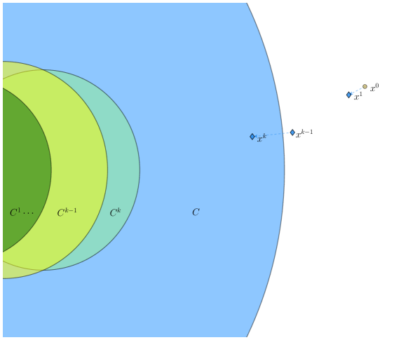
Figure 1: Sketch of PACA finite convergence.

We mention that, as far as we know, this is the first circumcenter-based method which is proved to be finitely convergent. The methods introduced in [18, 17] achieve superlinear convergence assuming that the convex sets have smooth boundaries; our convergence analysis requires no smoothness hypothesis.

Lemma 6.1.

Let $\{x^{k}\}$ be the sequence generated by PACA. Under the Slater condition given in Definition 2.1, if the sequence $\{x^{k}\}$ is infinite, then $\sum_{k=0}^{\infty}\epsilon_{k}<\infty$.

Proof 6.2.

Let $\delta_{k}\coloneqq\operatorname{dist}(x^{k},C^{k})$. By 5.8 in Proposition 5.7 and 5.10, we have

$$\delta_{k+1}\leq\lambda\delta_{k}\leq\dots\leq\lambda^{k-N}\delta_{N}$$

for all $k>N$. Let $z^{k}$ be the closest point to $x^{k}$ in $C^{k}$, so that $\delta_{k}=\left\lVert x^{k}-z^{k}\right\rVert$. Since $\{x^{k}\}$ is infinite, for all $k$ there exists $j(k)\in\{1,\ldots,m\}$ such that $f_{j(k)}(x^{k})>0$. On the other hand, $f_{j(k)}(z^{k})+\epsilon_{k}\leq 0$, because $z^{k}\in C^{k}$. Using the subgradient inequality, we have

$$f_{j(k)}(z^{k})\geq f_{j(k)}(x^{k})+\left(u^{j(k)k}\right)^{\top}(z^{k}-x^{k}).$$

Adding $\epsilon_{k}$ on both sides of 6.2, we obtain

$$0\geq f_{j(k)}(z^{k})+\epsilon_{k}\geq f_{j(k)}(x^{k})+\epsilon_{k}+\left(u^{j(k)k}\right)^{\top}(z^{k}-x^{k}),$$

Since $f_{j(k)}(x^{k})>0$, we get from 6.2

$$-\epsilon_{k}\geq\left(u^{j(k)k}\right)^{\top}(z^{k}-x^{k}),$$

because $f_{j(k)}(x^{k})>0$. In view of 6.2,

$$\epsilon_{k}\leq\left\lvert\left(u^{j(k)k}\right)^{\top}(z^{k}-x^{k})\right\rvert\leq\left\lVert u^{j(k)k}\right\rVert\,\left\lVert z^{k}-x^{k}\right\rVert=\left\lVert u^{j(k)k}\right\rVert\delta_{k}.$$

From 6.2 and 5.6, we get

$$\delta_{k}\geq\frac{\epsilon_{k}}{\left\lVert u^{j(k)k}\right\rVert}\geq\frac{\epsilon_{k}}{\sigma}.$$

Now 6.2 and 6.2 imply

$$\epsilon_{k}\leq\sigma\delta_{N}\lambda^{k-N},$$

for all $k>N$. Let $\zeta=\sum_{k=0}^{N-1}\epsilon_{k}$. From 6.2, we obtain

$$\sum_{k=0}^{\infty}\epsilon_{k}=\zeta+\sum_{k=N}^{\infty}\epsilon_{k}\leq\zeta+\sigma\delta_{N}\sum_{k=N}^{\infty}\lambda^{k-N}=\zeta+\frac{\sigma\delta_{N}}{1-\lambda}<\infty,$$

establishing the result.

Theorem 6.3.

Let $\{x^{k}\}$ be the sequence generated by PACA. Under the Slater condition given in Definition 2.1, if the sequence $\{\epsilon_{k}\}$ decreases to $0$ and $\sum_{k=0}^{\infty}\epsilon_{k}=\infty$, then PACA has finite termination, i.e., there exists some index $k$ such that $x^{k}$ solves CFP.

Proof 6.4.

Immediate from Lemma 6.1.

We observe that there are many choices for the sequence $\{\epsilon_{k}\}$ which satisfy the assumptions of Theorem 6.3, for instance, $\epsilon_{k}=\nu k^{-r}$, for any $\nu>0$ and any $r\in(0,1]$.

7 Numerical experiments

In order to investigate the behavior of PACA, we compare our proposed algorithm with two other approximate projections based algorithms: CRM on the Pierra’s reformulation with approximate projection (denoted as CARMprod) (see [4]), the Simultaneous subgredient projection method (SSPM) of [34], and the Modified Cyclic subgradient projection (MCSP) by [28].

Taking into account Theorem 6.3, we set the perturbation parameter for PACA defining $\epsilon_{k}\coloneqq\hat{\epsilon}(k)=\frac{1}{k}$ (algorithm PACA1) and $\epsilon_{k}\coloneqq\bar{\epsilon}(k)=\frac{1}{\sqrt{k}}$ (algorithm PACA2). Therefore, we ensure that PACA1 and PACA2 have finite termination.

We comment that SSPM is somehow similar to PACA: the difference relies on the way one set $\alpha_{k}$, instead of the one PACA uses. For PACA, $\alpha_{k}$ given in 2), which arises from a circumcenter (see Lemma 4.3). For SSPM, we set $\alpha_{k}=1$ and for MCSP, $\alpha_{k}=\frac{1}{k}$. Meanwhile, MCSP just computes its iterates visiting all sets by means of perturbed subgradients computed as in 2).

Likewise to PACA, SSPM and MCSP also enforce a perturbation parameter, and thus SSPM1 and MCSP1 employ $\epsilon_{k}\coloneqq\hat{\epsilon}(k)$, while SSPM2 and MCSP1 use $\epsilon_{k}\coloneqq\bar{\epsilon}(k)$.

These methods are applied to the problem of finding a point in the intersection of $m$ ellipsoids, i.e, in Section 1, each $C_{i}\coloneqq\xi_{i}$ is regarded as an ellipsoid given by

$$\xi_{i}\coloneqq\left\{x\in\mathds{R}^{n}\mid f_{i}(x)\leq 0,\text{ for }i=1,2,\ldots,m\right\},$$

with $f_{i}:\mathds{R}^{n}\rightarrow\mathds{R}$ defined as $f_{i}(x)\coloneqq x^{\top}A_{i}x+2x^{\top}b^{i}-c_{i}.$ For each $i=1,\ldots,m$, $A_{i}\in\mathds{R}^{n\times n}$ is symmetric positive definite, $b^{i}$ is a vector, and $c_{i}$ is a positive scalar.

The ellipsoids are generated in accordance to [17, Section 5], so that the sets have not only nonempty intersection, but also a Slater point. Moreover, the subdifferential of each $f_{i}$ is a singleton given by $\partial f_{i}(x)=\{2(A_{i}x+b^{i})\}$, since each $f_{i}$ is differentiable.

The computational experiments were performed on an Intel Xeon W-2133 3.60GHz with 32GB of RAM running Ubuntu 20.04 using Julia v1.9 [25], and are fully available at https://github.com/lrsantos11/CRM-CFP.

Figures 2, 1, and 2 summarize the results for different number of ellpsoids ($m$) and dimensions ($n$). Figure 2 is a Dolan and Moré [31] performance profile that depict benchmark different methods on a set of problems with respect to a performance measure, CPU Time in our case. Table 1 shows the average CPU Time per dimension and number of ellipsoids. Table 2 shows the statistics of all the experiments with Ellipsoids intersection considering CPU Time. Our numerical results indicate the PACA framework as the winner, with PACA2 being the fastest algorithm.

Note that the numerical experiments also portray the finite convergence inherent to PACA, MCSP and SSPM, as the solutions found by all the algorithms PACA1, PACA2, MCSP1, MCSP2, SSPM1 and SSPM2 are interior.

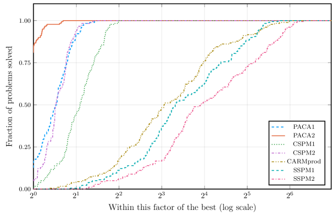
Figure 2: Performance profile of the experiments Ellipsoids intersection considering CPU Time ().

Table 1: The average of CPU Time ($\times\qty{e-4}{}$) per dimension ($n$) and number of Ellipsoids ($m$).

$n$	$m$	PACA1	PACA2	CSPM1	CSPM2	CARMprod	SSPM1	SSPM2
20	5	$0.000\,174\,969$	$0.000\,130\,767$	$0.000\,229\,563$	$0.000\,284\,64$	$0.001\,003\,89$	$0.000\,657\,018$	$0.000\,802\,294$
20	10	$0.000\,149\,423$	$0.000\,116\,902$	$0.000\,249\,496$	$0.000\,182\,543$	$0.001\,720\,9$	$0.001\,145\,04$	$0.001\,732\,75$
20	20	$0.000\,451\,726$	$0.000\,329\,275$	$0.000\,744\,147$	$0.000\,517\,616$	$0.006\,185\,17$	$0.004\,964\,54$	$0.007\,860\,01$
50	5	$0.000\,177\,545$	$0.000\,180\,787$	$0.000\,254\,27$	$0.000\,276\,673$	$0.000\,791\,727$	$0.000\,738\,637$	$0.000\,929\,345$
50	10	$0.000\,358\,364$	$0.000\,304\,642$	$0.000\,561\,542$	$0.000\,467\,513$	$0.002\,103\,98$	$0.002\,367\,45$	$0.003\,454\,41$
50	20	$0.001\,050\,21$	$0.000\,717\,103$	$0.001\,378\,14$	$0.000\,984\,226$	$0.009\,027\,02$	$0.010\,613\,9$	$0.016\,144\,6$
100	5	$0.002\,067\,47$	$0.002\,021\,06$	$0.002\,694\,07$	$0.002\,171\,55$	$0.005\,549\,36$	$0.008\,651\,19$	$0.009\,481\,01$
100	10	$0.004\,647\,27$	$0.003\,732\,48$	$0.004\,506\,96$	$0.003\,561\,53$	$0.022\,821\,5$	$0.024\,529\,5$	$0.031\,684\,6$
100	20	$0.033\,966\,9$	$0.027\,872\,8$	$0.028\,340\,4$	$0.036\,367\,3$	$0.881\,335$	$0.344\,371$	$0.375\,855$

Table 2: Statistics of all the experiments with Ellipsoids intersection considering CPU Time ($\times\qty{e-4}{}$).

	mean	median	min	max
PACA1	$0.004\,782\,65$	$0.000\,380\,431$	$2.321\,51\text{\times}{10}^{-5}$	$0.544\,721$
PACA2	$0.003\,933\,98$	$0.000\,294\,468$	$2.956\,95\text{\times}{10}^{-5}$	$0.434\,008$
MCSPM1	$0.004\,328\,74$	$0.000\,611\,745$	$5.084\,08\text{\times}{10}^{-5}$	$0.409\,626$
MCSPM2	$0.004\,979\,29$	$0.000\,405\,281$	$4.128\,74\text{\times}{10}^{-5}$	$0.558\,935$
CARMprod	$0.103\,393$	$0.002\,194\,81$	$0.000\,211\,971$	$16.0615$
MSSPM1	$0.044\,226\,5$	$0.003\,042\,16$	$0.000\,106\,17$	$5.322\,59$
MSSPM2	$0.049\,771\,6$	$0.004\,124\,24$	$0.000\,156\,793$	$5.416\,55$

8 Concluding remarks

In this work, we introduced a novel algorithm called Perturbed Approximate Circumcenter Algorithm (PACA) to address the Convex Feasibility Problem (CFP). The proposed algorithm ensures finite convergence under a Slater condition, making it unique in the landscape of circumcenter schemes for CFP. In addition to yieding fininte convergence, this method leverages projections onto perturbed halfspaces, which are explicitly computed in contrast to obtaining general orthogonal projections onto convex set. Numerical experiments further showcase PACA’s efficiency compared to existing methods.

References

- [1] F. J. Aragón Artacho, R. Campoy, and M. K. Tam, The Douglas–Rachford algorithm for convex and nonconvex feasibility problems, Math Meth Oper Res, 91 (2020), https://doi.org/10.1007/s00186-019-00691-9.
- [2] F. J. Aragón Artacho, Y. Censor, and A. Gibali, The cyclic Douglas–Rachford algorithm with r-sets-Douglas–Rachford operators, Optimization Methods and Software, 34 (2018), pp. 875–889, https://doi.org/10.1080/10556788.2018.1504049.
- [3] G. H. M. Araújo, Circumcentering outer-approximate projections and reflections for the convex feasibility problem, master’s thesis, EMAp/Fundação Getúlio Vargas, Rio de Janeiro, BR, Mar. 2021.
- [4] G. H. M. Araújo, R. Arefidamghani, R. Behling, Y. Bello-Cruz, A. Iusem, and L.-R. Santos, Circumcentering approximate reflections for solving the convex feasibility problem, Fixed Point Theory and Algorithms for Sciences and Engineering, 2022 (2022), p. 30, https://doi.org/10.1186/s13663-021-00711-6, https://arxiv.org/abs/2105.00497.
- [5] R. Arefidamghani, Circumcentered-Reflection Methods for the Convex Feasibility Problem and the Common Fixed-Point Problem for Firmly Nonexpansive Operators, PhD thesis, IMPA, Rio de Janeiro, 2022.
- [6] R. Arefidamghani, R. Behling, Y. Bello-Cruz, A. N. Iusem, and L.-R. Santos, The circumcentered-reflection method achieves better rates than alternating projections, Comput. Optim. Appl., 79 (2021), pp. 507–530, https://doi.org/10.1007/s10589-021-00275-6, https://arxiv.org/abs/2007.14466.
- [7] R. Arefidamghani, R. Behling, A. N. Iusem, and L.-R. Santos, A circumcentered-reflection method for finding common fixed points of firmly nonexpansive operators, Journal of Applied and Numerical Optimization, (to appear) (2023), https://arxiv.org/abs/2203.02410.
- [8] H. H. Bauschke, J.-Y. Bello-Cruz, T. T. A. Nghia, H. M. Phan, and X. Wang, The rate of linear convergence of the Douglas–Rachford algorithm for subspaces is the cosine of the Friedrichs angle, Journal of Approximation Theory, 185 (2014), pp. 63–79, https://doi.org/10.1016/j.jat.2014.06.002.
- [9] H. H. Bauschke, J.-Y. Bello-Cruz, T. T. A. Nghia, H. M. Phan, and X. Wang, Optimal Rates of Linear Convergence of Relaxed Alternating Projections and Generalized Douglas-Rachford Methods for Two Subspaces, Numer. Algorithms, 73 (2016), pp. 33–76, https://doi.org/10.1007/s11075-015-0085-4.
- [10] H. H. Bauschke and J. M. Borwein, On the convergence of von Neumann’s alternating projection algorithm for two sets, Set-Valued Analysis, 1 (1993), pp. 185–212, https://doi.org/10.1007/BF01027691.
- [11] H. H. Bauschke and J. M. Borwein, On Projection Algorithms for Solving Convex Feasibility Problems, SIAM Review, 38 (1996), pp. 367–426, https://doi.org/10.1137/S0036144593251710.
- [12] H. H. Bauschke, H. Ouyang, and X. Wang, On circumcenters of finite sets in Hilbert spaces, Linear and Nonlinear Analysis, 4 (2018), pp. 271–295, https://arxiv.org/abs/1807.02093.
- [13] H. H. Bauschke, H. Ouyang, and X. Wang, Circumcentered methods induced by isometries, Vietnam Journal of Mathematics, 48 (2020), pp. 471–508, https://doi.org/10.1007/s10013-020-00417-z, https://arxiv.org/abs/1908.11576.
- [14] H. H. Bauschke, H. Ouyang, and X. Wang, On circumcenter mappings induced by nonexpansive operators, Pure and Applied Functional Analysis, 6 (2021), pp. 257–288, https://arxiv.org/abs/1811.11420.
- [15] H. H. Bauschke, H. Ouyang, and X. Wang, On the linear convergence of circumcentered isometry methods, Numer Algor, 87 (2021), pp. 263–297, https://doi.org/10.1007/s11075-020-00966-x, https://arxiv.org/abs/1912.01063.
- [16] H. H. Bauschke, H. Ouyang, and X. Wang, Best approximation mappings in Hilbert spaces, Math. Program., 195 (2022), pp. 855–901, https://doi.org/10.1007/s10107-021-01718-y, https://arxiv.org/abs/2006.02644.
- [17] R. Behling, Y. Bello-Cruz, A. Iusem, D. Liu, and L.-R. Santos, A successive centralized circumcenter reflection method for the convex feasibility problem, Comp. Appl. Math., (2023), https://doi.org/10.1007/s10589-023-00516-w, https://arxiv.org/abs/2212.06911.
- [18] R. Behling, Y. Bello-Cruz, A. N. Iusem, and L.-R. Santos, On the centralization of the circumcentered-reflection method, Math. Program., (2023), https://doi.org/10.1007/s10107-023-01978-w, https://arxiv.org/abs/2111.07022.
- [19] R. Behling, Y. Bello-Cruz, H. Lara-Urdaneta, H. Oviedo, and L.-R. Santos, Circumcentric directions of cones, Optim. Lett., 17 (2023), pp. 1069–1081, https://doi.org/10.1007/s11590-022-01923-4, https://arxiv.org/abs/2112.08314.
- [20] R. Behling, Y. Bello-Cruz, and L.-R. Santos, Circumcentering the Douglas–Rachford method, Numer. Algorithms, 78 (2018), pp. 759–776, https://doi.org/10.1007/s11075-017-0399-5, https://arxiv.org/abs/1704.06737.
- [21] R. Behling, Y. Bello-Cruz, and L.-R. Santos, On the linear convergence of the circumcentered-reflection method, Oper. Res. Lett., 46 (2018), pp. 159–162, https://doi.org/10.1016/j.orl.2017.11.018, https://arxiv.org/abs/1711.08651.
- [22] R. Behling, Y. Bello-Cruz, and L.-R. Santos, The block-wise circumcentered–reflection method, Comput. Optim. Appl., 76 (2020), pp. 675–699, https://doi.org/10.1007/s10589-019-00155-0, https://arxiv.org/abs/1902.10866.
- [23] R. Behling, Y. Bello-Cruz, and L.-R. Santos, Infeasibility and error bound imply finite convergence of alternating projections, SIAM J. Optim., 31 (2021), pp. 2863–2892, https://doi.org/10.1137/20M1358669, https://arxiv.org/abs/2008.03354.
- [24] R. Behling, Y. Bello-Cruz, and L.-R. Santos, On the Circumcentered-Reflection Method for the Convex Feasibility Problem, Numer. Algorithms, 86 (2021), pp. 1475–1494, https://doi.org/10.1007/s11075-020-00941-6, https://arxiv.org/abs/2001.01773.
- [25] J. Bezanson, A. Edelman, S. Karpinski, and V. B. Shah, Julia: A Fresh Approach to Numerical Computing, SIAM Review, 59 (2017), pp. 65–98, https://doi.org/10.1137/141000671.
- [26] G. Cimmino, Calcolo approssimato per le soluzioni dei sistemi di equazioni lineari, La Ricerca Scientifica, 9 (1938), pp. 326–333.
- [27] P. L. Combettes, The Convex Feasibility Problem in Image Recovery, in Advances in Imaging and Electron Physics, P. W. Hawkes, ed., vol. 95, Elsevier, San Diego, Jan. 1996, pp. 155–270, https://doi.org/10.1016/S1076-5670(08)70157-5.
- [28] A. R. De Pierro and A. N. Iusem, A finitely convergent “row-action” method for the convex feasibility problem, Appl Math Optim, 17 (1988), pp. 225–235, https://doi.org/10.1007/BF01448368.
- [29] N. Dizon, J. Hogan, and S. Lindstrom, Circumcentered reflections method for wavelet feasibility problems, ANZIAMJ, 62 (2022), pp. C98–C111, https://doi.org/10.21914/anziamj.v62.16118, https://arxiv.org/abs/2005.05687.
- [30] N. D. Dizon, J. A. Hogan, and S. B. Lindstrom, Circumcentering Reflection Methods for Nonconvex Feasibility Problems, Set-Valued Var. Anal, 30 (2022), pp. 943–973, https://doi.org/10.1007/s11228-021-00626-9.
- [31] E. D. Dolan and J. J. Moré, Benchmarking optimization software with performance profiles, Mathematical Programming, 91 (2002), pp. 201–213, https://doi.org/10.1007/s101070100263.
- [32] J. Douglas and H. H. Rachford Jr., On the numerical solution of heat conduction problems in two and three space variables, Transactions of the American Mathematical Society, 82 (1956), pp. 421–421, https://doi.org/10.1090/S0002-9947-1956-0084194-4.
- [33] Y. Hu, C. Li, and X. Yang, On Convergence Rates of Linearized Proximal Algorithms for Convex Composite Optimization with Applications, SIAM J. Optim., 26 (2016), pp. 1207–1235, https://doi.org/10.1137/140993090.
- [34] A. N. Iusem and L. Moledo, A finitely convergent method of simultaneous subgradient projections for the convex feasibility problem, Matemática Aplicada e Computacional, 5 (1986), pp. 169–184.
- [35] S. Kaczmarz, Angenäherte Auflösung von Systemen linearer Gleichungen, Bull. Int. Acad. Pol. Sci. Lett. Class. Sci. Math. Nat. A, 35 (1937), pp. 355–357.
- [36] A. Y. Kruger, D. R. Luke, and N. H. Thao, Set regularities and feasibility problems, Math. Program., 168 (2018), pp. 279–311, https://doi.org/10.1007/s10107-016-1039-x.
- [37] S. B. Lindstrom, Computable centering methods for spiraling algorithms and their duals, with motivations from the theory of Lyapunov functions, Comput Optim Appl, 83 (2022), pp. 999–1026, https://doi.org/10.1007/s10589-022-00413-8, https://arxiv.org/abs/2001.10784.
- [38] H. Ouyang, Circumcenter operators in Hilbert spaces, master’s thesis, University of British Columbia, Okanagan, CA, 2018, https://doi.org/10.14288/1.0371095.
- [39] H. Ouyang, Circumcentered Methods and Generalized Proximal Point Algorithms, PhD thesis, University of British Columbia, Kelowna, BC, 2022, https://doi.org/10.14288/1.0416335.
- [40] H. Ouyang, Finite convergence of locally proper circumcentered methods, Journal of Convex Analysis, 29 (2022), pp. 857–892, https://arxiv.org/abs/2011.13512.
- [41] H. Ouyang, Bregman circumcenters: Monotonicity and forward weak convergence, Optim Lett, 17 (2023), pp. 121–141, https://doi.org/10.1007/s11590-022-01881-x, https://arxiv.org/abs/2105.02308.
- [42] H. Ouyang and X. Wang, Bregman Circumcenters: Basic Theory, J Optim Theory Appl, 191 (2021), pp. 252–280, https://doi.org/10.1007/s10957-021-01937-5, https://arxiv.org/abs/2104.03234.
- [43] G. Pierra, Decomposition through formalization in a product space, Mathematical Programming, 28 (1984), pp. 96–115, https://doi.org/10.1007/BF02612715.
- [44] L. Qi, Complete Closedness of Maximal Monotone Operators, Mathematics of OR, 8 (1983), pp. 315–317, https://doi.org/10.1287/moor.8.2.315.
- [45] J. Wang, Y. Hu, C. Li, and J.-C. Yao, Linear convergence of CQ algorithms and applications in gene regulatory network inference, Inverse Problems, 33 (2017), p. 055017, https://doi.org/10.1088/1361-6420/aa6699.