Enumerating Safe Regions in Deep Neural Networks
with Provable Probabilistic Guarantees

Abstract

Identifying safe areas is a key point to guarantee trust for systems that are based on Deep Neural Networks (DNNs). To this end, we introduce the AllDNN-Verification problem: given a safety property and a DNN, enumerate the set of all the regions of the property input domain which are safe, i.e., where the property does hold. Due to the #P-hardness of the problem, we propose an efficient approximation method called $\epsilon$-ProVe. Our approach exploits a controllable underestimation of the output reachable sets obtained via statistical prediction of tolerance limits, and can provide a tight —with provable probabilistic guarantees— lower estimate of the safe areas. Our empirical evaluation on different standard benchmarks shows the scalability and effectiveness of our method, offering valuable insights for this new type of verification of DNNs.

Introduction

Deep Neural Networks (DNNs) have emerged as a groundbreaking technology revolutionizing various fields ranging from autonomous navigation (Tai, Paolo, and Liu 2017; Marzari et al. 2022) to image classification (O’Shea and Nash 2015) and robotics for medical applications (Corsi et al. 2023). However, while DNNs can perform remarkably well in different scenarios, their reliance on massive data for training can lead to unexpected behaviors and vulnerabilities in real-world applications. In particular, DNNs are often considered ”black-box” systems, meaning their internal representation is not fully transparent. A crucial DNNs weakness is the vulnerability to adversarial attacks (Szegedy et al. 2013; Amir et al. 2023), wherein small, imperceptible modifications to input data can lead to wrong and potentially catastrophic decisions when deployed.

To this end, Formal Verification (FV) of DNNs (Katz et al. 2017; Liu et al. 2021) holds great promise to provide assurances on the safety aspect of these functions before the actual deployment in real scenarios. In detail, the decision version of the DNN-Verification problem takes as input a trained DNN $\mathcal{N}$ and a safety property, typically expressed as an input-output relationship for $\mathcal{N}$, and aims at determining whether there exists at least an input configuration which results in a violation of the safety property. It is crucial to point out that due to the fact that the DNN’s input is typically defined in a continuous domain any empirical evaluation of a safety property cannot rely on testing all the (infinitely many) possible input configurations.

In contrast, FV can provide provable assurances on the DNNs’ safety aspect. However, despite the considerable advancements made by DNN-verifiers over the years (Katz et al. 2019; Wang et al. 2021; Liu et al. 2021), the binary result (safe or unsafe) provided by these tools is generally not sufficient to gain a comprehensive understanding of these functions. For instance, when comparing two neural networks and employing a FV tool that yields a unsafe answer for both (i.e., indicating the existence of at least one violation point) we cannot distinguish whether one model exhibits only a small area of violation around the identified counterexample, while the other may have multiple and widespread violation areas.

To overcome this limitation, a quantitative variant of FV, asking for the number of violation points, has been proposed and analyzed, first in (Baluta et al. 2019) for the restricted class of Binarized Neural Networks (BNNs) and more recently in (Marzari et al. 2023) for general DNNs. Following (Marzari et al. 2023) we will henceforth refer to such counting problem as #DNN-Verification. Due to the #P-Completeness of the #DNN-Verification, both studies in (Baluta et al. 2019; Marzari et al. 2023), focus on efficient approximate solutions, which allow the resolution of large-scale real-world problems while providing provable (probabilistic) guarantees regarding the computed count.

Solutions to the #DNN-Verification problem allow to estimate the probability that a DNN violates a given property but they do not provide information on the actual input configurations that are safe or violations for the property of interest.

On the other hand, knowledge of the distribution of safe and unsafe areas in the input space is a key element to devise approaches that can enhance the safety of DNNs, e.g., by patching unsafe areas through re-training.

To this aim, we introduce the AllDNN-Verification problem , which corresponds to computing the set of all the areas that do not result in a violation for a given DNN and a safety property (i.e., enumerating all the safe areas of a property’s input domain). The AllDNN-Verification is at least as hard as #DNN-Verification, i.e., it is easily shown to be #P-Hard.

Hence, we propose $\epsilon$-ProVe, an approximation approach that provides provable (probabilistic) guarantees on the returned areas. $\epsilon$-ProVe is built upon interval analysis of the DNN output reachable set and the iterative refinement approach (Wang et al. 2018b), enabling efficient and reliable enumeration of safe areas.

Notice that state-of-the-art FV methods typically propose an over-approximated output reachable set, thereby ensuring the soundness of the result. Nonetheless, the relaxation of the nonlinear activation functions employed to compute the over-approximate reachable set has non-negligible computational demands. In contrast, $\epsilon$-ProVe provides a scalable solution based on an underestimation of the output reachable set that exploits the Statistical Prediction of Tolerance Limits (Wilks 1942). In particular, we demonstrate how, with a confidence $\alpha$, our underestimation of the reachable set computed with $n$ random input configurations sampled from the initial property’s domain $A$ is a correct output reachable set for at least a fraction $R$ of an indefinitely large further sample of points. Broadly speaking, this result tells us that if all the input configurations obtained in a random sample produce an output reachable set that does not violate the safety property (i.e., a safe output reachable set) then, with probability $\alpha$, at least a subset of $A$ of size $R\cdot|A|$ is safe (i.e., $R$ is a lower bound on the safe rate in $A$ with confidence $\alpha$).

In summary, the main contributions of this paper are the following:

• We initiate the study of the AllDNN-verification problem, the enumeration version of the DNN-Verification

• Due to the #P-hardness of the problem, we propose $\epsilon$-ProVe a novel polynomial approximation method to obtain a provable (probabilistic) lower bound of the safe zones within a given property’s domain.

• We evaluate our approach on FV standard benchmarks, showing that $\epsilon$-ProVe is scalable and effective for real-world scenarios.

Preliminaries

In this section, we discuss existing FV approaches and related key concepts on which our approach is based. In contrast to the standard robustness and adversarial attack literature (Carlini and Wagner 2017; Madry et al. 2017; Zhang et al. 2022b), FV of DNNs seeks formal guarantees on the safety aspect of the neural network given a specific input domain of interest. Broadly speaking, if a DNN-Verification tool states that the region is provably verified, this implies that there are no adversarial examples – violation points – in that region. We recall in the next section the formal definition of the satisfiability problem for DNN-Verification (Katz et al. 2017).

DNN-Verification

Figure 1: A counterexample for a toy DNN-Verification problem.

In the DNN-Verification, we have as input a tuple $\mathcal{T}=\langle\mathcal{N},\mathcal{P},\mathcal{Q}\rangle$, where $\mathcal{N}$ is a DNN, $\mathcal{P}$ is precondition on the input, and $\mathcal{Q}$ a postcondition on the output. In particular, $\mathcal{P}$ denotes a particular input domain or region for which we require a particular postcondition $\mathcal{Q}$ to hold on the output of $\mathcal{N}$. Since we are interested in discovering a possible counterexample, $\mathcal{Q}$ typically encodes the negation of the desired behavior for $\mathcal{N}$. Hence, the possible outcomes are SAT if there exists an input configuration that lies in the input domain of interest, satisfying the predicate $\mathcal{P}$, and for which the DNN satisfies the postcondition $\mathcal{Q}$, i.e., at least one violation exists in the considered area, UNSAT otherwise.

To provide the reader with a better intuition on the DNN-Verification problem, we discuss a toy example.

Example 1.

(DNN-Verification) Suppose we want to verify that for the toy DNN $\mathcal{N}$ depicted in Fig. 1 given an input vector $x=(x_{1},x_{2})\in[0,1]\times[0,1]$, the resulting output should always be $y\geq 0$. We define $\mathcal{P}$ as the predicate on the input vector $x=(x_{1},x_{2})$ which is true iff $x\in[0,1]\times[0,1]$, and $\mathcal{Q}$ as the predicate on the output $y$ which is true iff $y=\mathcal{N}(x)<0,$ that is, we set $\mathcal{Q}$ to be the negation of our desired property. As reported in Fig. 1, given the vector $x=(1,0)$ we obtain $y<0$, hence the verification tool returns a SAT answer, meaning that a specific counterexample exists and thus the original safety property does not hold.

#DNN-Verification

Despite the provable guarantees and the advancement that formal verification tools have shown in recent years (Liu et al. 2021; Katz et al. 2019; Wang et al. 2021; Zhang et al. 2022a), the binary nature of the result of the DNN-Verification problem may hide additional information about the safety aspect of the DNNs. To address this limitation in (Marzari et al. 2023) the authors introduce the #DNN-Verification, i.e., the extension of the decision problem to its counting version. In this problem, the input is the same as the decision version, but we denote as $\Gamma(\mathcal{T})$ the set of all the input configurations for $\mathcal{N}$ satisfying the property defined by $\mathcal{P}$ and $\mathcal{Q},$ i.e.

$$\Gamma(\mathcal{T})=\Bigg{\{}x\;\big{|}\;\mathcal{P}(x)\wedge\mathcal{Q}(\mathcal{N}(x))\Bigg{\}}$$ (1)

Then, the #DNN-Verification consists of computing $|\Gamma(\mathcal{T})|$.

The approach (reported in Fig.2) solves the problem in a sound and complete fashion where any state-of-the-art FV tool for the decision problem can be employed to check each node of the Branch-and-Bound (Bunel et al. 2018) tree recursively. In detail, each node produces a partition of the input space into two equal parts as long as it contains both a point that violates the property and a point that satisfies it. The leaves of this recursion tree procedure correspond to partitioning the input space into parts where we have either complete violations or safety. Hence, the provable count of the safe areas is easily computable by summing up the cardinality of the subinput spaces in the leaves that present complete safety.

Clearly, by using this method, it is possible to exactly count (and even to enumerate) the safe points. However, due to the necessity of solving a DNN-Verification instance at each node (an intractable problem that might require exponential time), this approach becomes soon unfeasible and struggles to scale on real-world scenarios. In fact, it turns out that under standard complexity assumption, no efficient and scalable approach can return the exact set of areas in which a DNN is provably safe (as detailed in the next section).

To address this concern, after formally defining the AllDNN-Verification problem and its complexity, we propose first of all a relaxation of the problem, and subsequently, an approximate method that exploits the analysis of underestimated output reachable sets obtained using statistical prediction of tolerance limits (Wilks 1942) and provides a tight underapproximation of the safe areas with strong probabilistic guarantees.

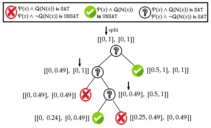
Figure 2: Explanatory image execution of exact count for a particular $\mathcal{N}$ and safety property.

The AllDNN-Verification Problem

The AllDNN-Verification problem asks for the set of all the safe points for a particular tuple $\langle\mathcal{N},\mathcal{P},\mathcal{Q}\rangle$.

Formally:

Definition 1 (AllDNN-Verification Problem).

abc

Input: A tuple $\mathcal{T}=\langle\mathcal{N},\mathcal{P},\mathcal{Q}\rangle$.

Output: the set of safe points $\Gamma(\mathcal{T}),$ as given in (1).

Considering the example of Fig. 2 solving the AllDNN-Verification problem for the safe areas consists in returning the set: $\displaystyle{\Gamma=\Bigg{\{}\big{[}[0.5,1],[0,1]\big{]}\cup\big{[}[0,0.24],[0,0.49]\big{]}\Bigg{\}}}.$

Hardness of AllDNN-Verification

From the #P-completeness of the #DNN-Verification problem proved in (Marzari et al. 2023) and the fact that exact enumeration also provides exact counting it immediately follows that the AllDNN-Verification is #P-hard, which essentially states that no polynomial algorithm is expected to exists for the AllDNN-Verification problem.

$\epsilon$-ProVe: a Provable (Probabilistic) Approach

In view of the structural scalability issue of any solution to the AllDNN-Verification problem, due to its #P-hardness, we propose to resort to an approximate solution. More precisely, we define the following approximate version of the AllDNN-Verification problem:

Definition 2 ($\epsilon$-Rectilinear Under-Approximation of safe areas for DNN ($\epsilon$-RUA-DNN)).

abc

Input: A tuple $\mathcal{T}=\langle\mathcal{N},\mathcal{P},\mathcal{Q}\rangle$.

Output: a family ${\cal R}=\{r_{1},\dots,r_{m}\}$ of disjoint rectilinear $\epsilon$-bounded hyperrectangles such that $\bigcup_{i}r_{i}\subseteq\Gamma({\cal T})$ and $|\Gamma({\cal T})\setminus\bigcup_{i}r_{i}|$ is minimum.

A rectilinear $\epsilon$-bounded hyperrectangle is defined as the cartesian product of intervals of size at least $\epsilon.$ Moreover, for $\epsilon>0,$ we say that a rectilinear hyperrectangle $r=\times_{i}[\ell_{i},u_{i}]$ is $\epsilon$-aligned if for each $i,$ both extremes $\ell_{i}$ and $u_{i}$ are a multiple of $\epsilon.$

The rational behind this new formulation of the problem is twofold: on the one hand, we are relaxing the request for the exact enumeration of safe points; on the other hand, we are requiring that the output is more concisely representable by means of hyperrectangles of some significant size.

Note that for $\epsilon\to 0$, $\epsilon$-RUA-DNN and AllDNN-Verification become the same problem. More generally, whenever the solution $\Gamma({\cal T})$ to an instance ${\cal T}$ of AllDNN-Verification can be partitioned into a collection of rectilinear $\epsilon$-bounded hyperrectangles, $\Gamma({\cal T})$ can be attained by an optimal solution for the $\epsilon$-RUA-DNN. This allows as to tackle the AllDNN-Verification problem via an efficient approach with strong probabilistic approximation guarantee to solve the $\epsilon$-RUA-DNN problem.

Our method is based on two main concepts: the analysis of an underestimated output reachable set with probabilistic guarantees and the iterative refinement approach (Wang et al. 2018b). In particular, in Fig. 3 we report a schematic representation of the approach that can be set up through reachable set analysis. Let us consider a possible domain for the safety property, i.e., the polygon highlighted in light blue in the upper left corner of Fig. 3.

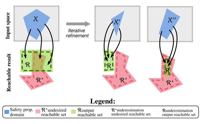
Figure 3: Explanatory image of how to exploit reachable set result for solving the AllDNN-Verification problem.

Suppose that the undesired output reachable set is the one highlighted in red called $\mathcal{R^{*}}$ in the bottom left part of the image, i.e., this set describes all the unsafe outcomes the DNN should never output starting from $\mathcal{X}$. Hence, in order to formally verify that the network respects the desired safety property, the output reachable set computed from the domain of the property (i.e., the green $\mathcal{R}$ area of the left side of the image) should have an empty intersection with the undesired reachable set (the red one). If this condition is not respected, as, e.g., in the left part of the figure, then there exists at least an input configuration for which the property is not respected.

To find all the portions of the property’s domain where either the undesired reachable set and the output reachable set are disjoint, i.e., $\mathcal{R^{*}}\bigcap\mathcal{R}=\emptyset$, or, dually, discover the unsafe areas where the condition $\mathcal{R}\subseteq\mathcal{R^{*}}$ holds (as shown in the right part of Fig. 3) we can exploit the iterative refinement approach (Wang et al. 2018b). However, given the nonlinear nature of DNNs, computing the exact output reachable set is infeasible. To address this issue, the reachable set is typically over-approximated, thereby ensuring the soundness of the result. Still, the relaxation of the nonlinear activation functions used to compute the over-approximated reachable set is computationally demanding.

In contrast, we propose a computationally efficient solution that uses underestimation of the reachable set and construct approximate solutions for the $\epsilon$-RUA-DNN problem with strong probabilistic guarantees.

Probabilistic Reachable Set

Given the complexity of computing the exact minimum and maximum of the function computed by a DNN, we propose to approximate the output reachable set using a statistical approach known as Statistical Prediction of Tolerance Limits (Wilks 1942).

We use a Monte Carlo sampling approach: for an appropriately chosen $n$, we sample $n$ input points and take the smallest and the greatest value achieved in the output node as the lower and the upper extreme of our probabilistic estimate of the reachable set. The choice of the sample size is based on the results of (Wilks 1942) that allow us to choose $n$ in order to achieve a given desired guarantee on the probability $\alpha$ that our estimate of the output reachable set holds for at least a fixed (chosen) fraction $R$ of a further possibly infinitely large sample of inputs. Crucially, this statistical result is independent of the probability function that describes the distribution of values in our function of interest and thus also applies to general DNNs. Stated in terms more directly applicable to our setting, the main result of (Wilks 1942) is as follows.

Lemma 1.

For any $R\in(0,1)$ and integer $n$, given a sample of $n$ values from a (continuous) set $X$ the probability that for at least a fraction $R$ of the values in a further possibly infinite sequence of samples from $X$ are all not smaller (respectively larger) than the minimum value (resp. maximum value) estimated with the first $n$ samples is given by the $\alpha$ satisfying the following equation

$$n\cdot\int_{R}^{1}x^{n-1}\;dx=\alpha$$ (2)

Computation of Safe Regions

We are now ready to give a detailed account of our algorithm $\epsilon$-ProVe.

Our approximation is based on the analysis of an underestimated output reachable set obtained by sampling a set of $n$ points $P_{A}$ from a domain of interest $A$. We start by observing that, it is possible to assume without loss of generality that the network has a single output node on whose reachable set we can verify the desired property (Liu et al. 2021). For networks not satisfying this assumption, we can enforce it by adding one layer. For example, consider the network in the example of Fig. 4 and suppose we are interested in knowing if, for a given input configuration in a domain $A=[0,1]\times[0,1]$, the output $y_{1}$ is always less than $y_{2}$. By adding a new output layer with a single node $y^{*}$ connected to $y_{1}$ by weight $-1$ and to $y_{2}$ with weight $1$ the condition required reduces to check that all the values in the reachable set for $y^{*}$ are positive.

In general, from the analysis of the underestimated reachable set of the output node computed as $\mathcal{R}=[min(y_{i}),max(y_{i})]\;\forall i=1,\dots,n$ we can obtain one of these three conditions:

$$\begin{cases}\text{$A$ is unsafe}\quad&\text{upper bound of }\mathcal{R}<0\\ \text{$A$ is safe}\quad&\text{lower bound of }\mathcal{R}\geq 0\\ unknown\quad&\text{otherwise}\end{cases}$$ (3)

Figure 4: Example of computation single reachable set for a DNN with two outputs.

With reference to the toy example in Figure 4, assuming we sample only $n=2$ input configurations, $(1,0)$ and $(0,1)$ which when propagated through $\mathcal{N}$ produce as a result in the new output layer the vector $y^{*}=[8,5]$. This results in the estimated reachable set $\mathcal{R}=[5,8]$. Since the lower bound of this interval is positive, we conclude that the region $A$, under consideration, is completely safe.

To confirm the correctness of our construction, we can check the partial values of the original output layer and notice that no input generates $y_{1}\geq y_{2}$. Specifically, if all inputs result in $y_{1}\geq y_{2}$ (violating the specification we are trying to verify), then the reachable set must have, by construction, a negative upper bound, leading to the correct conclusion that the area is unsafe. On the other hand, if only some inputs produce $y_{1}\geq y_{2}$, then we obtain a reachable set with a negative lower bound and a positive upper bound, thus we cannot state whether the area is unsafe or not, and we should proceed with an interval refinement process. Hence, this approach allows us to obtain the situations shown to the right of Fig. 3, that is, a situation in which the reachable set is either completely positive ($A$ safe) or completely negative ($A$ unsafe).

We present the complete pipeline of $\epsilon$-ProVe in Algorithm 1. Our approach receives as input a standard tuple for the DNN-Verification and creates the augmented DNN $\mathcal{N}^{\prime}$ (line 3) following the intuitions provided above. Moreover, we initialize respectively the set of safe regions as an empty set and the unchecked regions as the entire domain of the safety specification encoded in $\mathcal{P}$ (line 5).

Algorithm 1 $\epsilon$-ProVe

1:  Input: $\mathcal{T}=\langle\mathcal{N},\mathcal{P},\mathcal{Q}\rangle$, $n$ ($\#$ of samples to compute $\mathcal{R}$)

2:  Output: lower bound of the set of safe regions in $\mathcal{P}$.

3:  $\mathcal{N^{\prime}}\leftarrow\texttt{CreateAugmentedDNN}(\mathcal{N},\mathcal{P},\mathcal{Q})$

4:  safe_regions $\leftarrow\emptyset$

5:  unknown $\leftarrow\texttt{GetDomain}(\mathcal{P})$

6:  while (unknown $\neq\emptyset$) or $(\epsilon-precision$ not reached) do

7:     $A\leftarrow\texttt{GetAreaToVerify}$(unknown)

8:     $\mathcal{R}_{A}\leftarrow\texttt{ComputeReachableSet}(\mathcal{N}^{\prime},\;A,\;n)$

9:     if $\texttt{lower}(\mathcal{R}_{A})\geq 0$ then

10:        safe_regions $\leftarrow$ safe_regions $\cup\;A$

11:     else if $\texttt{upper}(\mathcal{R}_{A})<0$ then

12:        continue

13:     else

14:        unknown $\leftarrow$ unknown $\cup\;\texttt{IntervalRefinement}(A)$

15:     end if

16:  end while

17:  return safe_regions

Inside the loop (line 6), our approximation iteratively considers one area $A$ at the time and begins computing the reachable set, as shown above. We proceed with the analysis of the interval computed, where in case we obtain a positive reachable set, i.e., the lower bound is positive (lines 9-10), then the area under consideration is deemed as safe and stored in the set of safe regions we are enumerating. On the other hand, if the interval is negative, that is, the upper bound is negative, then we ignore the area and proceed (lines 11-12). Finally, if we are not in any of these cases, we cannot assert any conclusions about the nature of the region we are checking, and therefore we must proceed with splitting the area according to the heuristic we prefer (lines 13-14).

The loop ends when either we have checked all areas of the domain of interest, or we have reached the $\epsilon-precision$ on the iterative refinement. In detail, given the continuous nature of the domain, it is always possible to split an interval into two subparts, that is, the process could continue indefinitely in the worst case. For this reason, as is the case of other state-of-the-art FV methods that are based on this approach, we use a parameter to decide when to stop the process. This does not affect the correctness of the output since our goal is to (tightly) underapproximate the safe regions, and thus in case the $\epsilon-precision$ is reached, the area under consideration would not be considered in the set that the algorithm returns, thus preserving the correctness of the result. Although the level of precision can be set arbitrarily, it does have an effect on the performance of the method. In the supplementary material, we discuss the impact that different heuristics and different setting of hyper-parameters have on the resulting approximation.

Theoretical Guarantees

In this section, we analyze the theoretical guarantees that our approach can provide. We assume that the IntervalRefinement procedure consists of iteratively choosing one of the dimensions of the input domain and splitting the area into two halves of equal size as in (Wang et al. 2018b). The theoretical guarantee easily extends to any other heuristic provided that each split produces two parts both at least a fixed constant fraction $\beta$ of the subdivided area. Moreover, we assume that reaching the $\epsilon$ precision is implemented as testing that the area has reached size $\epsilon^{d},$ i.e., it is the cartesian product of $d$ intervals of size $\epsilon.$ It follows that, by definition, the areas output by $\epsilon$-ProVe are $\epsilon$-bounded and $\epsilon$-aligned.

The following proposition is the basis of the approximation guarantee (in terms of the size of the safe area returned) on the solution output by $\epsilon$-ProVe on an instance of the $\epsilon$-RUA-DNN problem.

Proposition 2.

Fix a real number $\epsilon>0,$ an integer $k\geq 3,$ and a real $\gamma>k\epsilon.$ Let $\cal T$ be an instance of the $\epsilon$-RUA-DNN problem. Then for any solution ${\cal R}=\{r_{1},\dots,r_{m}\}$ such that for each $i=1,\dots,m,$ $r_{i}$ is $\gamma$-bounded, there is a solution ${\cal R}^{(\epsilon)}=\{r_{1}^{(\epsilon)},\dots,r_{m}^{(\epsilon)}\}$ such that each $r_{i}^{(\epsilon)}$ is $\epsilon$-aligned and $||{\cal R}^{(\epsilon)}||\geq\left(\frac{k-2}{k}\right)^{d}||{\cal R}||,$ where $d$ is the number of dimensions of the input space, and for every solution ${\cal R}^{\prime}$, $||{\cal R}^{\prime}||=|\cup_{i}r_{i}|$ is the total area covered by the hyperrectangles in ${\cal R}^{\prime}$.

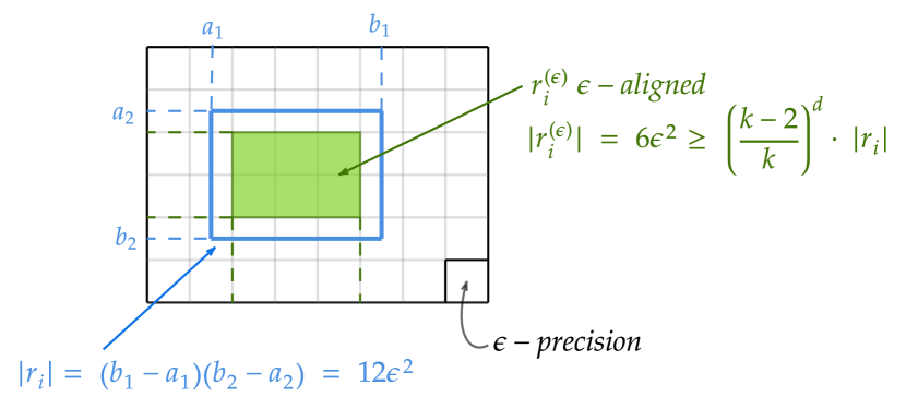
Figure 5: An Example of applying Lemma 3 with $k=3$.

The result is obtained by applying the following lemma to each hyperrectangle of the solution ${\cal R}.$

Lemma 3.

Fix a real number $\epsilon>0$ and an integer $k\geq 3.$ For any $\gamma>k\epsilon$ and any $\gamma$-bounded rectilinear hyperrectangle $r\subseteq\mathbb{R}^{d},$ there is a $\epsilon$-aligned rectilinear hyperrectangle $r^{(\epsilon)}$ such that: (i) $r^{(\epsilon)}\subseteq r$; and (ii) $|r^{(\epsilon)}|\geq\left(\frac{k-2}{k}\right)^{d}|r|.$

Fig. 5 gives a pictorial explanation of the lemma. In the example shown, $k=3$ and the parameter $\epsilon$ is the unit of the grid, which we can imagine superimposed to the bidimensional ($d=2$) space in which the hyperrectangles live. Hence $\gamma=3\epsilon.$ The non-$\epsilon$-aligned $r_{i}$ (depicted in blue) is $\gamma$-bounded, since its width $w=(b_{1}-a_{1})=4\epsilon$ and its height $h=(b_{2}-a_{2})=3\epsilon$ are both $\geq 3\epsilon.$ Hence, it covers completely at least $w-2$ columns and $h-2$ rows of the grid. These rows and columns define the green $\epsilon$-aligned hyperrectangle $r_{i}^{(\epsilon)},$ of dimension

$$\geq(w-2)\cdot(h-2)\geq\frac{k-2}{k}w\cdot\frac{k-2}{k}h=\left(\frac{k-2}{k}\right)^{d}|r_{i}|.$$

The following theorem summarizes the coverage approximation guarantee and the confidence guarantee on the safety nature of the areas returned by $\epsilon$-ProVe.

Theorem 4.

Fix a positive integer $d$ and real values $\epsilon,\alpha,R\in(0,1),$ with $R>1-\epsilon^{d}.$ Let ${\cal T}$ be an instance of the AllDNN-Verification with input in $[0,1]^{d},$ and let $k$ be the largest integer such that $\Gamma({\cal T})$ can be partitioned into $k\epsilon$-bounded rectilinear hyperrectangle. Let ${\cal R}^{(\epsilon)}=\{r_{i}^{(\epsilon)}\mid i=1,\dots,m\}$ be the set of areas returned by $\epsilon$-ProVe using $n$ samples at each iteration, with $n\geq\log_{R}(1-\alpha^{1/m}).$ Then,

1. (coverage guarantee) with probability $1-R^{n}$ the solution ${\cal R}^{(\epsilon)}$ is a $\left(\frac{k-2}{k}\right)^{d}$ approximation of $\Gamma({\cal T}),$ i.e., $||{\cal R}^{(\epsilon)}||\geq\left(\frac{k-2}{k}\right)^{d}|\Gamma({\cal T})|$;

2. (safety guarantee) with probability at least $\alpha$, in each hyperrectangle $r\in{\cal R}^{(\epsilon)}$ at most $(1-R)\cdot|r|$ points are not safe.

This theorem gives two types of guarantees on the solution returned by $\epsilon$-ProVe. Specifically, point 2. states that for any $R<1$ and $\alpha<1$, $\epsilon$-ProVe can guarantee that with probability $\alpha$ no more than $(1-R)$ of the points classified as safe can, in fact, be violations. Moreover, point 1. guarantees that, provided the space of safety points is not too scattered—formalized by the existence of some representation in $k\epsilon$-bounded hyperrectangles— the total area returned by $\epsilon$-ProVe is guaranteed to be close to the actual $\Gamma({\cal T}).$

Finally, the theorem shows that the two guarantees are attainable in an efficient way, providing a quantification of the size $n$ of the sample needed at each iteration. Note that the value of $m$ needed in defining $n$ can be either estimated, e.g., by a standard doubling technique, or it could be set using the upper limit $2^{d\log(1/\epsilon)}$, which is the maximum number of possible split operations performed before reaching the $\epsilon$ precision limit.

Proof.

(Sketch) The safety guarantee (item 2.) is a direct consequence of Lemma 1. In fact, an hyperrectangle $r$ is returned as safe if all the $n$ sampled points from $r$ are not violations, i.e., their output is $\geq 0$ (see (3)). By Lemma 1, at most $(1-R)$ of the points in $r$ can give an output $<0$, i.e., can be a violation, where, from the solution of (2),

$$\hat{\alpha}=(1-R^{n}).$$ (4)

Since samples are chosen independently in different hyperrectangles, this bound on the number of violations in a hyperrectangle of $\cal R^{(\epsilon)}$ holds simultaneously for all $m$ of them with probability ${\hat{\alpha}}^{m}.$ Taking $\alpha={\hat{\alpha}}^{m},$ and solving (4) for $n$ we get $n\geq\log_{R}(1-\alpha^{1/m})$ as desired.

For the coverage guarantee, we start by noticing that under the hypotheses on $k$, Proposition 2 guarantees the existence of a solution ${\cal R}^{\epsilon}_{1}$ made of $\epsilon$-bounded and $\epsilon$-aligned rectilinear hyperrectangles. Let ${\cal R}^{\epsilon}_{2}$ be a solution obtained from ${\cal R}^{\epsilon}_{1}$ by partitioning each hyperrectangle into pieces of minimum possible size $\epsilon^{d},$ each one $\epsilon$-aligned.

The first observation is that, being the solution produced by $\epsilon$-ProVe made of $\epsilon$-bounded and $\epsilon$-aligned rectilinear hyperrectangles, also ${\cal R}^{\epsilon}_{2}$ is among the solutions possibly returned by the algorithm.

We now observe that with probability $1-R^{n}$ each hyperrectangle $r^{\prime}$ in ${\cal R}^{\epsilon}_{2}$ must be contained in some hyperrectangle $r$ in the solution ${\cal R}^{(\epsilon)}$ returned by $\epsilon$-ProVe.

First note that if in the iterations of the execution of $\epsilon$-ProVe, $r^{\prime}$ keeps on being contained in an area where both safe and violation points are sampled, then eventually $r^{\prime}$ will become itself an area to analyze. At such a step, clearly every sample in $r^{\prime}$ will be safe and $r^{\prime}$ will be included in ${\cal R}^{(\epsilon)},$ as desired.

Therefore, the only possibility for $r^{\prime}$ not to be contained in any $r\in{\cal R}^{(\epsilon)}$ is that at some iteration an area $A\supseteq r^{\prime}$ is analyzed and all the $n$ points sampled in $A$ are violation points, so that the whole $A$ (including $r^{\prime}$) is discarded (as unsafe) by $\epsilon$-ProVe. However, by Lemma 1 with probability $(1-R^{n})$ this can happen only if $\epsilon^{d}=|r^{\prime}|<(1-R)|A|,$ which contradicts the hypotheses. Hence, with probability $(1-R^{n})$, the $r^{\prime}$ must be contained in a hyperrectangle of ${\cal R}^{(\epsilon)},$ concluding the argument. ∎

Instance	$\epsilon$-ProVe ($\alpha_{TOT}=99.9\%$)			Exact count or MC sampling		Und-estimation (% distance)
	# Safe regions	Safe rate	Time	Safe rate	Time
Model_2_20	335	78.50%	0.4s	79.1%	234min	0.74%
Model_2_56	251	43.69%	0.3s	44.46%	196min	1.75%
Model_MN_1	545	64.72%	60.6s	67.59%	0.6s	4.24%
Model_MN_2	1	100%	0.4s	100%	0.4s	-
$\phi_{2}$ ACAS Xu_2.1	2462	97.47%	26.9s	99.25%	0.6s	1.81%
$\phi_{2}$ ACAS Xu_3.3	1	100%	0.4s	100%	0.5s	-

Table 1: Comparison of $\epsilon$-ProVe and Exact count or Monte Carlo (MC) sampling approach on different benchmark setups. Full results and other different experiments are reported in the supplementary material.

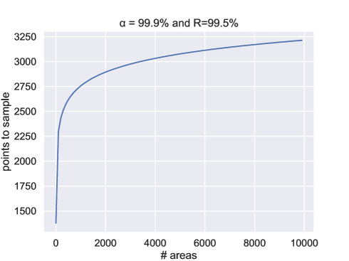
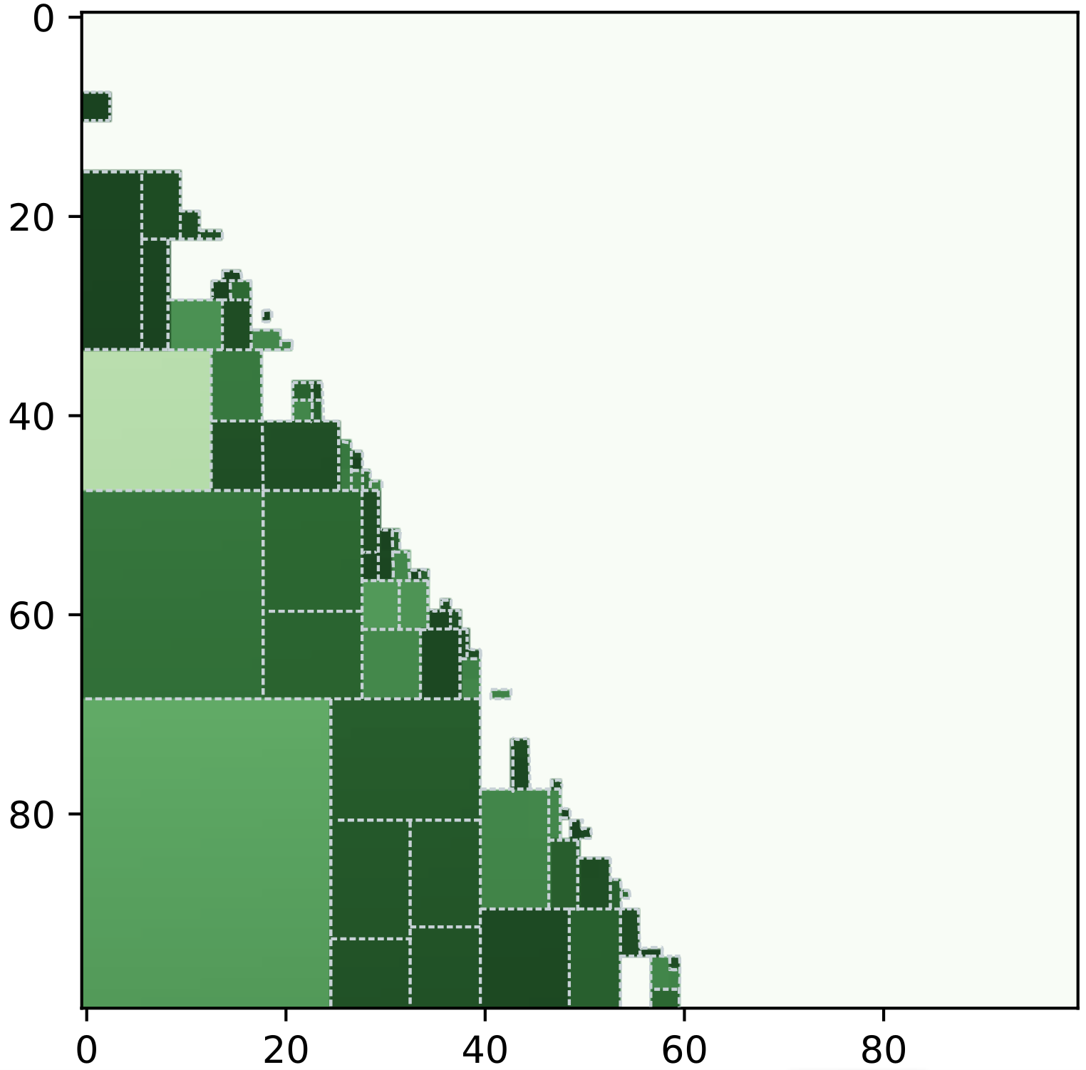
Figure 6: Left: Correlation point to sample and # of (un)safe areas using $\epsilon$-ProVe to obtain a confidence $\alpha=99.9\%$ and a lower bound $R=99.5\%$. Right: example of a set of safe regions (in green) returned by $\epsilon$-ProVe (scaled x100).

Fig. 6 (left) shows the correlation between the number of points to be sampled based on the number of areas obtained by $\epsilon$-ProVe if we want to obtain a total confidence of $\alpha=99.9\%$ and a lower bound $R=99.5\%$. As we can notice from the plot, if we compute our output reachable set sampling $n=3250$ points, we are able to obtain the desired confidence and lower bound if the number of regions is in $[1,10000]$. For this reason, in all our empirical evaluations, we use $n=3500$ to compute $\mathcal{R}$. An explanatory example of the possible result achievable using our approach is depicted in Fig. 6 (right).

Empirical Evaluation

In this section, we evaluate the scalability of our approach, and we validate the theoretical guarantees discussed in the previous section. Our analysis considers both simple DNNs to analyze in detail the theoretical guarantees and two real-world scenarios to evaluate scalability. The first scenario is the ACAS xu (Julian et al. 2016), an airborne collision avoidance system for aircraft, which is a well-known standard benchmark for formal verification of DNNs (Liu et al. 2021; Katz et al. 2017; Wang et al. 2018a). The second scenario considers DNN trained and employed for autonomous mapless navigation tasks in a Deep Reinforcement Learning (DRL) context (Tai, Paolo, and Liu 2017; Marzari, Marchesini, and Farinelli 2023; Marchesini et al. 2023).

All the data are collected on a commercial PC equipped with an M2 Apple silicon. The code used to collect the results and several additional experiments and discussions on the impact of different heuristics for our approximation are available in the supplementary material.

Correctness and Scalability Experiments

These experiments aim to estimate the correctness and scalability of our approach. Specifically for each model tested, we used $\epsilon$-ProVe to return the set of safe regions in the domain of the property under consideration. All data are collected with parameters $\alpha_{TOT}=99.9\%$ and $R=99.5\%$ and $n=3500$ points to compute the reachable set used for the analysis. The results are presented in Table 1. For all experiments, we report the number of safe regions returned by $\epsilon$-ProVe (for which we also know the hyperrectangles position in the property domain), the percentage of safe areas relative to the total starting area (i.e., the safe rate), and the computation time. Moreover, we include a comparison, measured as percentage distance, of the safe rate computed with alternative methods, such as an exact enumeration method (whenever feasible due to the scalability issue discussed above) and a Monte Carlo (MC) Sampling approach using a large number of samples (i.e., 1 million). It’s important to note that the MC sampling only provides a probabilistic estimate of the safe rate, lacking information about the location of safe regions in the input domain.

The first block of Table 1 involves two-dimensional models with two hidden layers of 32 nodes activated with ReLU. The safety property consists of all the intervals of $\mathcal{P}$ in the range $[0,1]$ and a postcondition $\mathcal{Q}$ that encodes a strictly positive output. Notably, $\epsilon$-ProVe is able to return the set of safe regions in a fraction of a second, and the safe rate returned by our approximation deviates at most a $1.75\%$ from the one computed by an exact count, which shows the tightness of the bound returned by our approach. In the second block of Tab. 1, the Mapless Navigation (MN) DNNs are composed of 22 inputs, two hidden layers of 64 nodes activated with $ReLU$, and finally, an output space composed of five nodes, which encode the possible actions of the robot. We test a behavioral safety property where $\mathcal{P}$ encodes a potentially unsafe situation (e.g., there is an obstacle in front), and the postcondition $\mathcal{Q}$ specifies the unsafe action that should not be selected ($\bigvee_{i=2,3}y_{1}<y_{i}$ if $y_{1}$ encodes a forward movement). The table illustrates how increasing input space and complexity affects computation time. Nevertheless, the proposed approximation remains efficient even for ACAS xu tests, returning results within seconds. Crucially, focusing on $Model\_MN\_2$ and $\phi_{2}$ ACAS Xu_3.3, $\epsilon$-ProVe states that all the property’s domain is safe (i.e., no violation points). The correctness of the results was verified by employing VeriNet (Henriksen et al. 2021), a state-of-the-art FV tool.

Discussion

We studied the AllDNN-Verification, a novel problem in the area of FV of DNNs asking for the set of all the safe regions for a given safety property. Due to the #P-hardness of the problem, we proposed an approximation approach, $\epsilon$-ProVe, which is, to the best of our knowledge, the first method able to efficiently approximate the safe regions with some guarantees on the tightness of the solution returned. We believe $\epsilon$-ProVe is an important step to provide consistent and effective tools for analyzing safety in DNNs.

An interesting future direction could be testing the enumeration of the unsafe regions for subsequent patching or a safe retrain on the areas discovered by our approach.

Appendix A Supplementary Material

Full Proof of Theorem 4

Theorem 4.

Fix a positive integer $d$ and real values $\epsilon,\alpha,R\in(0,1),$ with $R>1-\epsilon^{d}.$ Let ${\cal T}$ be an instance of the AllDNN-Verification with input in $[0,1]^{d},$ and let $k$ be the largest integer such that $\Gamma({\cal T})$ can be partitioned into $k\epsilon$-bounded rectilinear hyperrectangle. Let ${\cal R}^{(\epsilon)}=\{r_{i}^{(\epsilon)}\mid i=1,\dots,m\}$ be the set of areas returned by $\epsilon$-ProVe using $n$ samples at each iteration, with $n\geq\log_{R}(1-\alpha^{1/m}).$ Then,

1. (coverage guarantee) with probability $1-R^{n}$ the solution ${\cal R}^{(\epsilon)}$ is a $\left(\frac{k-2}{k}\right)^{d}$ approximation of $\Gamma({\cal T}),$ i.e., $||{\cal R}^{(\epsilon)}||\geq\left(\frac{k-2}{k}\right)^{d}|\Gamma({\cal T})|$;

2. (safety guarantee) with probability at least $\alpha$, in each hyperrectangle $r\in{\cal R}^{(\epsilon)}$ at most $(1-R)\cdot|r|$ points are not safe.

Proof.

We start showing the safety guarantee (item 2.).
Each hyperrectangle $r_{i}\in\mathcal{R}^{(\epsilon)},\;\forall i=1,\dots,m$, returned by $\epsilon$-ProVe is deemed as safe if all the $n$ sampled points when propagated through the DNN $\mathcal{N}$ produce a strictly positive output reachable set, as shown in (3). By lemma 1, we have that the probability that a least a fraction $R$ in a further indefinitely larger sample exceeds the minimum value estimated in the first sample using $n$ sample is given by:

$$n\cdot\int_{R}^{1}x^{n-1}\;dx =\hat{\alpha}$$

$$x^{n}\Big{|}_{R}^{1} =\hat{\alpha}$$

$$(1-R^{n}) =\hat{\alpha}$$ (5)

which tells us that if all the $n$ input configurations sampled produce a positive reachable set, with probability $\hat{\alpha}$ at least a subset of $A$ of size $R\cdot|A|$ is safe, i.e., $R$ is a correct lower bound on the safe rate in $A$ with confidence $\hat{\alpha}$. Hence, since $R<1$, we have for the same lemma, and with the same probability $\hat{\alpha}$, that at most $(1-R)\cdot|A|$ is not safe. Moreover, since samples are chosen independently in different $r_{i}$, this bound on the unsafe rate in a hyperrectangle of $\mathcal{R}^{(\epsilon)}$ holds simultaneously for all $m$ of them with a probability equal to $\alpha=\prod_{i=1}^{m}\hat{\alpha}=\hat{\alpha}^{m}$. Solving equation (5) for $n$, we precisely get $n\geq\log_{R}(1-\alpha^{1/m})$ as desired.

We proceed to show the coverage guarantee (item 1.). Recalling the hypotheses on $k\geq 3$ of proposition 2, we have that given any solution for a tuple $\mathcal{T}$, $\mathcal{R}$ composed by $\gamma$-aligned hyperrectangles there also exists a solution $\mathcal{R}_{1}^{(\epsilon)}$ made of $r_{1},\dots,r_{m}$ $\epsilon$-aligned and $\epsilon$-bounded rectilinear hyperrectangles. In addition, applying lemma 3 to each $r_{i}$, we have that $||{\cal R}_{1}^{(\epsilon)}||\geq\left(\frac{k-2}{k}\right)^{d}||{\cal R}||,$ where $d$ is the number of dimensions of the input space. To show that this inequality holds, suppose to create a partition of each $r_{i}\in\mathcal{R}_{1}^{(\epsilon)}$ into pieces of minimum possible size, i.e., $|r_{i}^{{}^{\prime}}|=\epsilon^{d},\forall i=1,\dots,m$ and let us call this new set of $r_{i}^{{}^{\prime}}$, $\mathcal{R}_{2}^{(\epsilon)}$. The first observation is that this set, obtained by a solution produced by $\epsilon$-ProVe of $\epsilon$-bounded and $\epsilon$-aligned rectilinear hyperrectangles, is also among the possible solutions returned by the algorithm. More precisely, for each hyperrectangle $r_{i}^{{}^{\prime}}\in\mathcal{R}_{2}^{(\epsilon)}$, $\exists\;r_{i}$ of $\mathcal{R}_{1}^{(\epsilon)}$, such that $r_{i}^{{}^{\prime}}\subseteq r_{i}$. This relation holds since if in the iterations of $\epsilon$-ProVe, $r_{i}^{{}^{\prime}}\subseteq A$, where $A$ contains both safe and violation points, then eventually $r_{i}^{{}^{\prime}}$ will become itself, after the interval refinement process, an area to analyze. At such a step, since $r_{i}^{{}^{\prime}}$ is obtained from an original hyperrectangle $r_{i}$ deemed as safe, every sample in $r_{i}^{{}^{\prime}}$ will produce a positive reachable set, also deeming $r_{i}^{{}^{\prime}}$ safe and including it in ${\cal R}_{2}^{(\epsilon)}$, as desired.

Hence, the only possibility for $r_{i}^{{}^{\prime}}$ not to be contained in any $r_{i}\in{\cal R}_{1}^{(\epsilon)}$ is that, at some iteration, an area $A\supseteq r_{i}^{{}^{\prime}}$ is analyzed and all the $n$ points sampled in $A$ are violation points, so that the whole $A$ (including $r_{i}^{{}^{\prime}}$) is discarded (as unsafe) by $\epsilon$-ProVe. However, by lemma 1 with probability $(1-R^{n})$ this can happen only if $|r_{i}^{{}^{\prime}}|<(1-R)|A|,$ which, since we set $|r_{i}^{{}^{\prime}}|=\epsilon^{d}$, contradicts the hypotheses on $R$. Hence, with probability $(1-R^{n})$, $r_{i}^{{}^{\prime}}$ must be contained in a hyperrectangle of ${\cal R}_{1}^{(\epsilon)}$ showing that the following general inequality holds $||{\cal R}^{(\epsilon)}||\geq\left(\frac{k-2}{k}\right)^{d}|\Gamma({\cal T})|$.

∎

Impact of Heuristics on $\epsilon$-ProVe Performances

Although the correctness of the approximation does not depend on the heuristic chosen to split the input space under consideration (as shown in Theorem 4), we performed an additional experiment to understand its impact on the quality of the estimation. In particular, as shown in Alg. 1, the loop ends when either $\epsilon$-ProVe explores all the unknown regions, or it reaches a specific $\epsilon-precision$. Regarding the latter, all our results are given for the case of a maximum number of splits equal to $s=18$, since, in preliminary testing, this value has shown to give the best trade-off between efficiency and accuracy. Hence, with respect to theoretical analysis in Theorem 4), with this choice, we expect the solution returned by $\epsilon$-ProVe to be $\epsilon$-bounded, for some $\epsilon\in[2^{1/s},2^{d/s}]$ considering the maximum and the expected number of times that a split happens on the same dimension.

Moreover, another key aspect when using iterative refinement is the choice of the dimension (input coordinate) and the position where to perform the split. To this end, our sampling-based approach to estimating the reachable set also allows us to obtain some useful statistical measures, such as the mean and median of the samples in each dimension, that can be useful for the heuristics. More specifically, we tested the following five heuristics:

• H1: split the node along the bigger dimension, i.e., $d=argmax_{i=1}^{m}u_{i}-\ell_{i}$, with $u_{i}$ and $\ell_{i}$ the upper and lower bound of each interval, respectively. The split is performed in correspondence with the median value of the samples that result safe after the propagation through the DNN.

• H2: as H1, but the split is performed along the mean value of the safe samples.

• H3: select one dimension randomly, and the split is performed along the median value of the safe samples.

• H4: as H3, but the split is performed along the mean value of the safe samples.

• H5: select the dimension and the position to split based on the distribution of the safe and violation points, i.e., partitioning the input space into parts where we have as many as possible violation points in one part and safety in the other. We report a simplified example of this heuristic in Fig. 7. More specifically, let us suppose to have only two dimensions and to have sampled $n$ points that result in the situation depicted in Fig. 7. Hence, for each dimension, the heuristic seeks to find the splitting point that better divides the safe points from the unsafe (violation) ones. In this situation, the dimension chosen will be $x_{2}$ as it allows a better partition of the input space, splitting in correspondence with the dotted line, which represents the maximum value of the safe points along $x_{2}$.

  

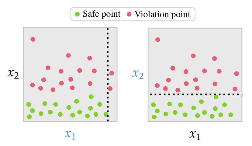
  Figure 7: Example of single test split on each dimension $x_{1},x_{2},$ (highlighted in blue) using $H5$ in a specific situation.

Instance	H1
	# Safe regions	Safe rate	Time
Model_2_20	731	78.91%	0.5s
Model_MN_3	1196	53.14%	1m21s
$\phi_{2}$ ACAS Xu_2.1	3540	97.32%	29.1s
	H2
	# Safe regions	Safe rate	Time
Model_2_20	678	79.01%	1.2s
Model_MN_3	739	53.08%	1m42s
$\phi_{2}$ ACAS Xu_2.1	1613	97.24%	39s
	H3
	# Safe regions	Safe rate	Time
Model_2_20	2319	78.63%	1.9s
Model_MN_3	-	-	-
$\phi_{2}$ ACAS Xu_2.1	22853	83%	4m20s
	H4
	# Safe regions	Safe rate	Time
Model_2_20	1757	78.8%	2.9s
Model_MN_3	-	-	-
$\phi_{2}$ ACAS Xu_2.1	31515	78.09%	5m
	H5
	# Safe regions	Safe rate	Time
Model_2_20	355	78.5%	0.4s
Model_MN_3	845	52.95%	1m15s
$\phi_{2}$ ACAS Xu_2.1	2462	97.47%	26.9s

Table 2: Comparison of different heuristic on $\epsilon$-Prove. ’-’ indicates a heuristic that requires more than 5 minutes. The target safe rates obtained using either an exact enumeration method (when possible) or a Monte Carlo estimation are: for model_2_20 79.1%, for model_MN_3 55.93% and finally for $\phi_{2}$ ACAS Xu_2.1 99.25%.

We have noticed that all these heuristics have roughly the same computational cost on a single split, and thus an improvement in the computation time of the complete execution of $\epsilon$-ProVe translates directly into the choice of better heuristics. We tested each heuristic on three different models with $\alpha=99.9\%,R=99.5\%$, and $n=3500$ samples. For each heuristic tested, we collected: the number of safe regions, the safe rate, and the computation time, respectively. Ideally, for a similar safe rate, the best heuristic should return the fewest regions (i.e., the best compact solution of the safe regions) in the lowest possible time. In Tab.2, we report the results obtained. As we can see, H5 is the best heuristic as it yields the best trade-off between the efficiency and compactness of the solution for all the models tested. We can notice that for $model\_MN\_3$ the improvement between $H2$ and $H5$ is not significant, we think this is due to the larger cardinality of the input space w.r.t the other models. Further experiments should be performed to devise better heuristics for these types of DNNs.

Full Results $\epsilon$-ProVe on Different Benchmarks

We report in Tab 4 the full results comparing $\epsilon$-ProVe on different benchmarks. As stated in the main paper, we consider three different setups: the first one is a set of small DNNs, the second one is a realistic set of Mapless Navigation (MN) DNNs, used in a DRL context, and finally, we used the standard FV benchmark ACAS xu(Julian et al. 2016). For the latter, we consider only a subset of the original 45 models. More precisely, based on the result of the second international Verification of Neural Networks (VNN) competition (Bak, Liu, and Johnson 2021), we test part of the models for which the property $\phi_{2}$ does not hold (i.e., the models that present at least one single input configuration that violates the safety property) and one single model ($\phi_{2}$ ACAS Xu_3.3) for which the property holds (i.e., 100% provable safe).

Hyperrectangle $r$	ProVe
	Violation rate
[[0.6999231, 1], [0, 0.2563121]]	0%
[[0.6999231, 1],[0.2563121, 0.40074086]]	0%
[[0.48361894, 0.6999231], [0, 0.18614466]]	0%
[[0.23474114, 0.34573981],[0, 0.09308449]]	0%
[[0.39214072, 0.39503244],[0.245827, 0.25156769]]	0.031%
[[0.95905697, 0.95924747], [0.60187447, 0.60229677]]	0.0488%

Table 3: Partial results of Prove (Corsi, Marchesini, and Farinelli 2021) on each single hyperrectangle $r$ returned as solution for the $\epsilon$-RUA-DNN for $model\_2\_68$. The csv file with full results is available in the supplementary material folder.

Instance	$\epsilon$-ProVe ($\alpha_{TOT}=99.9\%$)			Exact count or MC sampling		Und-estimation (% distance)
	# Safe regions	Safe rate	Time	Safe rate	Time
Model_2_20	335	78.50%	0.4s	79.1%	234min	0.74%
Model_2_56	251	43.69%	0.3s	44.46%	196min	1.75%
Model_2_68	252	31.07%	0.3s	31.72%	210min	2.07%
Model_MN_1	545	64.72%	60.6s	67.59%	0.6s	4.24%
Model_MN_2	1	100%	0.4s	100%	0.4s	-
Model_MN_3	845	52.95%	75.5s	55.93%	0.4s	5.33%
$\phi_{2}$ ACAS Xu_2.1	2462	97.47%	26.9s	99.25%	0.6s	1.81%
$\phi_{2}$ ACAS Xu_2.2	1990	97.12%	21.7s	98.66%	0.5s	1.56%
$\phi_{2}$ ACAS Xu_2.3	2059	96.77%	20.0s	98.22%	0.5s	1.47%
$\phi_{2}$ ACAS Xu_2.4	2451	97.97%	17.5s	99.09%	0.5s	1.13%
$\phi_{2}$ ACAS Xu_2.5	2227	95.72%	23.6s	98.19%	0.5s	2.51%
$\phi_{2}$ ACAS Xu_2.6	1745	97.46%	19.2s	98.79%	0.5s	1.34%
$\phi_{2}$ ACAS Xu_2.7	2165	95.69%	23.6s	97.35%	0.5s	1.7%
$\phi_{2}$ ACAS Xu_2.8	1101	97.52%	9.0s	98.06%	0.5s	0.55%
$\phi_{2}$ ACAS Xu_2.9	767	99.24%	6.7s	99.7%	0.5s	0.47%
$\phi_{2}$ ACAS Xu_3.1	1378	97.37%	13.1s	98.15%	0.5s	0.79%
$\phi_{2}$ ACAS Xu_3.3	1	100%	0.4s	100%	0.5s	-
$\phi_{2}$ ACAS Xu_3.4	1230	99.03%	9.3s	99.53%	0.5s	0.49%
$\phi_{2}$ ACAS Xu_3.5	1166	98.39%	8.0s	98.9%	0.5s	0.51%
$\phi_{2}$ ACAS Xu_3.6	1823	96.34%	20.8s	98.17%	0.4s	1.86%
$\phi_{2}$ ACAS Xu_3.7	1079	98.16%	11.1s	99.82%	0.5s	0.66%
$\phi_{2}$ ACAS Xu_3.8	1854	97.97%	17.0s	99.09%	0.5s	1.12%
$\phi_{2}$ ACAS Xu_3.9	1374	95.96%	17.6s	97.34%	0.5s	1.43%
$\phi_{2}$ ACAS Xu_4.1	1205	98.91%	10.1s	99.6%	0.5s	0.67%
$\phi_{2}$ ACAS Xu_4.3	2395	97.38%	18.9s	98.56%	0.5s	1.2%
$\phi_{2}$ ACAS Xu_4.4	2693	97.99%	17.7s	99%	0.5s	1.04%
$\phi_{2}$ ACAS Xu_4.5	1733	97.24%	16.2s	98.2%	0.5s	1.01%
$\phi_{2}$ ACAS Xu_4.6	1843	96.72%	17.0s	97.74%	0.5s	1.04%
$\phi_{2}$ ACAS Xu_4.7	1923	96.34%	25.7s	98.17%	0.5s	1.86%
$\phi_{2}$ ACAS Xu_4.8	1996	95.53%	22.3s	98.14%	0.5s	1.64%
$\phi_{2}$ ACAS Xu_4.9	601	99.62%	4.3s	99.85%	0.5s	0.23%
$\phi_{2}$ ACAS Xu_5.1	2530	97.77%	16.5s	98.72%	0.5s	0.97%
$\phi_{2}$ ACAS Xu_5.2	2496	96.59%	27.7s	98.92%	0.5s	2.36%
$\phi_{2}$ ACAS Xu_5.4	2875	97.83%	21.6s	99.13%	0.5s	1.31%
$\phi_{2}$ ACAS Xu_5.5	1660	97.07%	15.1s	98.03%	0.5s	0.97%
$\phi_{2}$ ACAS Xu_5.6	1909	97.06%	14.7s	97.94%	0.5s	0.89%
$\phi_{2}$ ACAS Xu_5.7	1452	96.15%	16.2s	97.2%	0.5s	1.09%
$\phi_{2}$ ACAS Xu_5.8	2357	95.15%	27.5s	97.74%	0.5s	2.65%
$\phi_{2}$ ACAS Xu_5.9	1494	97.13%	10.9s	97.83%	0.5s	0.71%
$\phi_{3}$ ACAS Xu_1.3	1	100%	0.7s	100%	0.6s	-
$\phi_{3}$ ACAS Xu_1.4	1	100%	0.7s	100%	0.6s	-
$\phi_{3}$ ACAS Xu_1.5	1	100%	0.7s	100%	0.6s	-
						Mean: 1.27%

Table 4: Comparison of $\epsilon$-ProVe and Exact count or Monte Carlo (MC) sampling approach on different benchmark setups.

Moreover, to further validate the correctness of our approximation, we also performed a final experiment on property $\phi_{3}$ of the same benchmark. This property is particularly interesting as it holds for most of the 45 models (as shown in (Bak, Liu, and Johnson 2021)). In particular, in this scenario we tested only models for which the property holds, i.e., we expect a 100% of safe rate for each model tested. For simplicity, in Tab. 4, we report only the first three models tested for $\phi_{3}$ since the results were similar for all the DNNs evaluated. As expected, we empirically confirmed that also for this particular situation, $\epsilon$-ProVe returns a correct solution.

From the results of Tab 4, we can see that our approximation returns a tight, safe rate (mean of underestimation 1.27%) for each model tested in at most half a minute, confirming the effectiveness and correctness of our approach.

#DNN-Verification on $\epsilon$-ProVe Result

We performed an empirical experiment using an exact count method to confirm the safety probability guarantee of Theorem 4. Specifically, theorem 4 proves that$\epsilon$-ProVe returns with probability $\alpha$ a set of safe areas ${\cal R}^{(\epsilon)}$, where for each hyperrectangle $r\in{\cal R}^{(\epsilon)}$ at most $(1-R)\cdot|r|$ points are not safe. This experiment aims to empirically verify this safety guarantee with a formal method. To this end, we rely on ProVe (Corsi, Marchesini, and Farinelli 2021), an exact count method that returns the violation rate, i.e., the portion of the area that presents violation points in a given domain of interest.

Due to scalability issues of exact counters, discussed in detail in the main paper, we only perform this evaluation on each of the $252$ hyperrectangles returned by $\epsilon$-ProVe for the $model\_2\_68$. The formal results are reported in Tab. 3.

The exact count method used on each hyperrectangle $r$ returned by $\epsilon$-ProVe confirms the correctness of our approach. Since we set $R=99.5\%$ as a provable safe lower bound guaranteed, we expected at most a $0.05\%$ violation rate on each hyperrectangle $r_{i}$. Crucially, we notice that for only $2$ of $252$ hyperrectangles tested, we have a violation rate over the $0\%$, and this value is strictly less than $0.05\%$. Hence, also this experiment confirms the strong probabilistic guarantee presented in point 2. of Theorem 4.

References

- Amir et al. (2023) Amir, G.; Corsi, D.; Yerushalmi, R.; Marzari, L.; Harel, D.; Farinelli, A.; and Katz, G. 2023. Verifying learning-based robotic navigation systems. In 29th International Conference, TACAS 2023, 607–627. Springer.
- Bak, Liu, and Johnson (2021) Bak, S.; Liu, C.; and Johnson, T. 2021. The second international verification of neural networks competition (vnn-comp 2021): Summary and results. arXiv preprint arXiv:2109.00498.
- Baluta et al. (2019) Baluta, T.; Shen, S.; Shinde, S.; Meel, K. S.; and Saxena, P. 2019. Quantitative Verification of Neural Networks and Its Security Applications. In Proceedings of the 2019 ACM SIGSAC Conference on Computer and Communications Security.
- Bunel et al. (2018) Bunel, R. R.; Turkaslan, I.; Torr, P.; Kohli, P.; and Mudigonda, P. K. 2018. A unified view of piecewise linear neural network verification. Advances in Neural Information Processing Systems, 31.
- Carlini and Wagner (2017) Carlini, N.; and Wagner, D. 2017. Towards evaluating the robustness of neural networks. In 2017 ieee symposium on security and privacy (sp), 39–57. Ieee.
- Corsi, Marchesini, and Farinelli (2021) Corsi, D.; Marchesini, E.; and Farinelli, A. 2021. Formal verification of neural networks for safety-critical tasks in deep reinforcement learning. In Uncertainty in Artificial Intelligence, 333–343. PMLR.
- Corsi et al. (2023) Corsi, D.; Marzari, L.; Pore, A.; Farinelli, A.; Casals, A.; Fiorini, P.; and Dall’Alba, D. 2023. Constrained reinforcement learning and formal verification for safe colonoscopy navigation. In 2023 IEEE/RSJ International Conference on Intelligent Robots and Systems (IROS). IEEE.
- Henriksen et al. (2021) Henriksen, P.; et al. 2021. DEEPSPLIT: An Efficient Splitting Method for Neural Network Verification via Indirect Effect Analysis. In IJCAI, 2549–2555.
- Julian et al. (2016) Julian, K. D.; Lopez, J.; Brush, J. S.; Owen, M. P.; and Kochenderfer, M. J. 2016. Policy compression for aircraft collision avoidance systems. In 2016 IEEE/AIAA 35th Digital Avionics Systems Conference (DASC), 1–10. IEEE.
- Katz et al. (2017) Katz, G.; Barrett, C.; Dill, D. L.; Julian, K.; and Kochenderfer, M. J. 2017. Reluplex: An efficient SMT solver for verifying deep neural networks. In International conference on computer aided verification, 97–117. Springer.
- Katz et al. (2019) Katz, G.; Huang, D. A.; Ibeling, D.; Julian, K.; Lazarus, C.; Lim, R.; Shah, P.; Thakoor, S.; Wu, H.; Zeljić, A.; et al. 2019. The marabou framework for verification and analysis of deep neural networks. In International Conference on Computer Aided Verification.
- Liu et al. (2021) Liu, C.; Arnon, T.; Lazarus, C.; Strong, C.; Barrett, C.; Kochenderfer, M. J.; et al. 2021. Algorithms for verifying deep neural networks. Foundations and Trends® in Optimization, 4(3-4): 244–404.
- Madry et al. (2017) Madry, A.; Makelov, A.; Schmidt, L.; Tsipras, D.; and Vladu, A. 2017. Towards deep learning models resistant to adversarial attacks. arXiv preprint arXiv:1706.06083.
- Marchesini et al. (2023) Marchesini, E.; Marzari, L.; Farinelli, A.; and Amato, C. 2023. Safe Deep Reinforcement Learning by Verifying Task-Level Properties. In nternational Conference on Autonomous Agents and Multiagent Systems (AAMAS).
- Marzari et al. (2023) Marzari, L.; Corsi, D.; Cicalese, F.; and Farinelli, A. 2023. The #DNN-Verification problem: Counting Unsafe Inputs for Deep Neural Networks. In International Joint Conference on Artificial Intelligence (IJCAI).
- Marzari et al. (2022) Marzari, L.; Corsi, D.; Marchesini, E.; and Farinelli, A. 2022. Curriculum learning for safe mapless navigation. In Proceedings of the 37th ACM/SIGAPP Symposium on Applied Computing, 766–769.
- Marzari, Marchesini, and Farinelli (2023) Marzari, L.; Marchesini, E.; and Farinelli, A. 2023. Online Safety Property Collection and Refinement for Safe Deep Reinforcement Learning in Mapless Navigation. In International Conference on Robotics and Automation (ICRA).
- O’Shea and Nash (2015) O’Shea, K.; and Nash, R. 2015. An introduction to convolutional neural networks. arXiv preprint arXiv:1511.08458.
- Szegedy et al. (2013) Szegedy, C.; Zaremba, W.; Sutskever, I.; Bruna, J.; Erhan, D.; Goodfellow, I.; and Fergus, R. 2013. Intriguing properties of neural networks. arXiv preprint arXiv:1312.6199.
- Tai, Paolo, and Liu (2017) Tai, L.; Paolo, G.; and Liu, M. 2017. Virtual-to-real DRL: Continuous control of mobile robots for mapless navigation. In IROS.
- Wang et al. (2018a) Wang, S.; Pei, K.; Whitehouse, J.; Yang, J.; and Jana, S. 2018a. Efficient formal safety analysis of neural networks. Advances in Neural Information Processing Systems, 31.
- Wang et al. (2018b) Wang, S.; Pei, K.; Whitehouse, J.; Yang, J.; and Jana, S. 2018b. Formal security analysis of neural networks using symbolic intervals. In 27th USENIX Security Symposium (USENIX Security 18), 1599–1614.
- Wang et al. (2021) Wang, S.; Zhang, H.; Xu, K.; Lin, X.; Jana, S.; Hsieh, C.-J.; and Kolter, J. Z. 2021. Beta-crown: Efficient bound propagation with per-neuron split constraints for neural network robustness verification. Advances in Neural Information Processing Systems, 34: 29909–29921.
- Wilks (1942) Wilks, S. S. 1942. Statistical prediction with special reference to the problem of tolerance limits. The annals of mathematical statistics, 13(4): 400–409.
- Zhang et al. (2022a) Zhang, H.; Wang, S.; Xu, K.; Li, L.; Li, B.; Jana, S.; Hsieh, C.-J.; and Kolter, J. Z. 2022a. General cutting planes for bound-propagation-based neural network verification. Advances in Neural Information Processing Systems, 35: 1656–1670.
- Zhang et al. (2022b) Zhang, H.; Wang, S.; Xu, K.; Wang, Y.; Jana, S.; Hsieh, C.-J.; and Kolter, Z. 2022b. A branch and bound framework for stronger adversarial attacks of relu networks. In International Conference on Machine Learning, 26591–26604. PMLR.