Achieving quantum metrological performance and exact Heisenberg limit precision through superposition of $s$-spin coherent states

Résumé

In quantum phase estimation, the Heisenberg limit provides the ultimate accuracy over quasi-classical estimation procedures. However, realizing this limit hinges upon both the detection strategy employed for output measurements and the characteristics of the input states. This study delves into quantum phase estimation using $s$-spin coherent states superposition. Initially, we delve into the explicit formulation of spin coherent states for a spin $s=3/2$. Both the quantum Fisher information and the quantum Cramer–Rao bound are meticulously examined. We analytically show that the ultimate measurement precision of spin cat states approaches the Heisenberg limit, where uncertainty decreases inversely with the total particle number. Moreover, we investigate the phase sensitivity introduced through operators $e^{i\zeta{S}_{z}}$, $e^{i\zeta{S}_{x}}$ and $e^{i\zeta{S}_{y}}$, subsequently comparing the resultants findings. In closing, we provide a general analytical expression for the quantum Cramer-Rao boundary applied to these three parameter-generating operators, utilizing general $s$-spin coherent states. We remarked that attaining Heisenberg-limit precision requires the careful adjustment of insightful information about the geometry of $s$-spin cat states on the Bloch sphere. Additionally, as the number of $s$-spin increases, the Heisenberg limit decreases, and this reduction is inversely proportional to the $s$-spin number.

I Introduction

Quantum metrology holds a pivotal role across a spectrum of technological domains [1, 2, 3, 4, 5, 6, 7, 8, 9, 10]. Within the realm of quantum information, metrology strives to achieve heightened precision measurements utilizing quantum resources in quantum states such as coherent states, entangled states, and compressed states [11, 12]. Its primary objective lies in refining the precision available for estimating physical parameters and transcending the confines of the standard quantum limit. This field has illuminated the potential of quantum metrology in devising measurement techniques that outperform classical counterparts in terms of precision [13, 14, 15]. As a consequence, leveraging quantum effects like quantum entanglement leads to a reduction in fluctuations by a factor proportional to $1/N$, referred to as the Heisenberg limit. In essence, the Heisenberg limit defines the ultimate precision threshold attainable through measurement [16, 34]. Consequently, advancements in precision can be realized through the utilization of exquisitely sensitive interferometric setups, such as the Mach-Zehnder interferometer involving $N$ entangled particles [18, 19]. Furthermore, non-classical states like entangled coherent states (ECS) and generalized NOON states exhibit analogous enhancements in accuracy [20, 21, 22, 23]. The Heisenberg limit can similarly be approached through the application of spin compressed states and spin coherent states [24, 25]. Spin coherent states emerge as crucial entities in quantum metrology, offering a means to measure physical quantities with superior precision compared to classical methodologies. These states confer numerous benefits to quantum metrology, including heightened sensitivity to external fields, diminished measurement noise, and the potential for meticulous preparation with high coherence [26, 27, 28]. These advantages collectively render spin coherent states a valuable asset for the precise measurement of diverse physical quantities across a wide array of applications.

Quantum metrology with coherent state superposition represents an advanced technique that enables more precise measurements compared to those achieved using simple coherent states [29, 30]. This method leverages the quantum properties of particles to make exceedingly accurate measurements. By employing spin coherent state superposition, it becomes feasible to ascertain magnetic fields with heightened precision compared to classical techniques. Similarly, these states find utility in quantifying phase parameters, such as rotation angles or polarizations. Within the realm of estimation theory, resolving a parameter estimation challenge entails the discovery of an estimator, denoted as $\hat{\zeta}$. This estimator functions as an operation that furnishes a collection of measurement outcomes within the parameter space. Furthermore, the attainment of utmost precision hinges on the quantum Fisher information, a critical factor for establishing the quantum Cramer-Rao bound [31, 32]. The most effective estimators are those that reach the limit set by this Cramer-Rao inequality:

$${\rm Var}(\hat{\zeta})\geq\frac{1}{nF(\zeta)},$$ (1)

where ${\rm Var}(\cdot)$ represents the variance, $n$ denotes the number of repeated experiments, $\hat{\zeta}$ is the estimator for the parameter $\zeta$, and $F(\zeta)$ stands for the Quantum Fisher Information (QFI). The QFI of a state $\rho_{\zeta}$ is defined as [31, 32]

$$F(\zeta)=Tr[\rho_{\zeta}L_{\zeta}^{2}].$$ (2)

Here, the operator denoted as $L_{\zeta}$ is commonly referred to as the symmetric logarithmic derivative operator, and its explicit determination is established through the following relation

$$\frac{\partial{\rho}_{\zeta}}{\partial{\zeta}}=\frac{{L_{\zeta}}{\rho_{\zeta}}+{\rho_{\zeta}}{L_{\zeta}}}{2}.$$ (3)

Certainly, the QFI plays a pivotal role within the realm of quantum metrology. Its utility extends to extracting insights about parameters that are not directly measurable, as indicated in [32]. Notably, this metric serves as a gauge for quantifying the phase sensitivity of quantum systems, as demonstrated in [33, 34, 35]. Importantly, it’s worth noting that this metric can be directly derived when the explicit calculation of the symmetric logarithmic derivative operator is performed. For mixed states [36, 37], the QFI can be expressed by utilizing the spectral decomposition of the output state $\rho_{\zeta}=\sum_{i=1}^{s}p_{i}{{|\Psi_{i}\rangle}{\langle{\Psi_{i}|}}}$, where $s$, $p_{i}$, and $|{\Psi_{i}}\rangle$ represent the dimension of the support for the matrix, the eigenvalues, and the eigenstates of $\rho_{\zeta}$, respectively. Then the QFI can be expressed by

$$F(\zeta)=\sum_{i=1}^{s}{\frac{1}{p_{i}}}(\partial_{\zeta}p_{i})^{2}+{\sum_{i=1}^{s}{4p_{i}\langle{\partial_{\zeta}\Psi_{i}|\partial_{\zeta}\Psi_{i}}\rangle}}-{\sum_{i,j=1}^{s}{\frac{8p_{i}p_{j}}{p_{i}+p_{j}}}{|\langle{\Psi_{i}|\partial_{\zeta}\Psi_{j}}\rangle}|^{2}}.$$ (4)

For the unitary parameterization process $\rho_{\zeta}=e^{-i{\zeta}H}{\rho}e^{+i{\zeta}H}$, with $H$ a Hermitian operator, the expression of the QFI reduces to

$$F(\zeta)={\sum_{i=1}^{s}{4p_{i}\langle{\Psi_{i}|H^{2}|\Psi_{i}}\rangle}}-{\sum_{i,j=1}^{s}{\frac{8p_{i}p_{j}}{p_{i}+p_{j}}}{|\langle{\Psi_{i}|H|\Psi_{j}}\rangle}|^{2}}.$$ (5)

Furthermore, for pure quantum states $\rho_{\zeta}=|{\Psi_{\zeta}}\rangle{\langle}\Psi_{\zeta}|$, the QFI is given by

$$F(\rho_{\zeta})=4[\langle{\Psi}|H^{2}|{\Psi}\rangle-|\langle{\Psi}|H|{\Psi\rangle}|^{2}]=4\Delta^{2}H,$$ (6)

where $H$ is the Hamiltonian that generates the interaction between the probe and the object being measured.

In this paper, we focus on the phase estimation protocol in quantum metrology, specifically centered around the task of estimating an unknown parameter $\zeta$ in the context of a $3/2$-spin system that involves the superposition of spin coherent states. We commence our exploration in Section (II) by establishing the groundwork through the introduction of spin coherent states. Subsequently, in Section (III), we delve into the calculation of both the quantum Fisher information and the quantum Cramer–Rao bound. We initiate our calculations by determining the quantum Fisher information and the quantum Cramer–Rao bound for scenarios wherein the system accumulates a phase via operations $e^{i\zeta{S}_{z}}$, $e^{i\zeta{S}_{x}}$, and $e^{i\zeta{S}_{y}}$. Specifically, we explore circumstances where optimal estimation of the phase shift parameter can be attained. Additionally, we showcase the substantial enhancement in measurement precision achievable through the utilization of a superposition of spin coherent states. Moving forward to Section (IV), we offer a comprehensive analytical expression for Fisher’s quantum information linked to the Cramer-Rao boundary of an unknown parameter, applicable to coherent states of any $s$-spin. Finally, our insights culminate in Section (V) where we provide our concluding remarks.

II A brief review on spin coherent states

Spin coherent states play a pivotal role in the characterization and utilization of the quantum properties exhibited by spin systems. These distinctive states, often labeled as Bloch states, embody a coherent superposition of diverse spin states within Hilbert space [38, 39, 40]. They furnish an elegant and potent mathematical portrayal of a particle’s spin orientation, thereby facilitating a deeper comprehension of the quantum intricacies underlying spin precession and evolution. Notably, the hallmark of spin-coherent states lies in their capacity to minimize the uncertainty inherent in measuring spin orientation. Their coherently structured essence engenders distributional attributes that evenly encompass the entirety of the Bloch sphere, bestowing heightened sensitivity to even the slightest deviations in spin angles. This feature makes them exceptionally suitable for applications in the realm of quantum metrology, where high-precision measurements are needed to accurately estimate unknown parameters. Broadly, coherent states exhibit numerous intriguing properties that have positioned them as the ”classical states” of the harmonic oscillator [41, 42, 43]. The coherent state $|\alpha{\rangle}$ of a quantum harmonic oscillator, characterized by the complex number $\alpha$, is given by

$$|{\alpha}\rangle=\exp{\left(-\frac{1}{2}|\alpha|^{2}\right)}\sum_{n=0}^{+\infty}{\frac{{\alpha}^{n}}{\sqrt{n!}}|n\rangle}$$ (7)

The fundamental goals of this study encompass the exploration of spin coherent states (SU(2) coherent states) and their associated quantum metrological capabilities. Here, we elucidate the key characteristics inherent to spin coherent states. These states [44], alternatively referred to as Bloch coherent states or atomic states, are defined by

$$\begin{split}|\theta,\varphi,s\rangle&=R(\theta,\varphi)|s,-s\rangle\\ &=\exp{[}\frac{-\theta}{2}(S_{+}e^{-i{\varphi}}-S_{-}e^{i{\varphi}})]|s,-s\rangle\\ &=\sum_{m=-s}^{s}C_{m}(\theta)e^{-{i(s+m)\varphi}}|s,m\rangle.\end{split}$$ (8)

with ${C_{m}(\theta)=\sqrt{\frac{2s!}{(s+m)!(s-m)!}}{\cos^{s-m}({\frac{\theta}{2}})}\sin^{s+m}({\frac{\theta}{2}})}$, ${|s,m\rangle}$ denotes the Dicke state; symmetric superpositions of states involving $N$ spins, with $s+m$ particles in one state and $s-m$ particles in the other, where $s=N/2$, $m=-s,-s+1,...,s-1,s$, and $R(\theta,\varphi)$ represents the rotation operator. The overlap between two spin coherent states is given by

$$\langle{\theta_{1},\varphi_{1},s}|{\theta_{2},\varphi_{2},s}\rangle=\Bigl{(}\cos{(\frac{\theta_{1}}{2})}\cos{(\frac{\theta_{2}}{2})}+e^{i({\varphi_{1}}-{{\varphi_{2}}})}\sin{(\frac{\theta_{1}}{2})}\sin{(\frac{\theta_{2}}{2})}\Bigl{)}^{2s}.$$ (9)

The parameters $\varphi$ and $\theta$ are, respectively, the azimuthal and polar coordinates on the Bloch sphere, $S_{-}$ and $S_{+}$ are often called lowering and raising operators. A collection of $N$ two-state bosons, symmetrical by particle exchange, is analogous to a system with $N/2$ angular momentum. Within this framework, the link between the basis of two-mode bosonic harmonic oscillators and the Dicke basis becomes apparent through an examination of the Schwinger representation of the $SU(2)$ algebra within the context of the two-mode Hilbert space, given by

$$S_{+}=\hat{a}^{\dagger}\hat{b},\hskip 28.45274ptS_{-}=\hat{b}^{\dagger}\hat{a},\hskip 28.45274ptS_{z}=\frac{1}{2}\left(\hat{a}^{\dagger}\hat{a}-\hat{b}^{\dagger}\hat{b}\right),$$ (10)

satisfying the commutation relations

$$[{S_{+},S_{-}}]=2S_{z},\hskip 28.45274pt[{S_{z},S_{\pm}}]={\pm}S_{\pm},$$ (11)

where $\hat{a}$ and $\hat{b}$ denote the annihilation operators corresponding to the first and second modes of the bosonic harmonic oscillator. This realization, which finds applicability in diverse scenarios, leads us to refer to these operators as the photon annihilation operators. When the combined photon count in the two modes $\hat{a}$ and $\hat{b}$ totals $N$, with $s=N/2$ and $m=\left(N_{a}-N_{b}\right)/2$, the Dicke basis can be represented as $\left|N_{a}\right\rangle\left|N_{b}\right\rangle\equiv\left|s,m\right\rangle$ (with $N=N_{a}+N_{b}$). These generators act on an irreducible unitary representation as follows

$$S_{\pm}|s,m\rangle=\sqrt{s(s+m)-m(m{\pm}1)}|s,m{\pm}1\rangle,\hskip 28.45274ptS_{z}|s,m\rangle=m|s,m\rangle,$$ (12)

and the Casimir operator is the quadratic operator $S^{2}$ which commutes with the operators $S_{\pm}$ and $S_{z}$. From $S_{\pm}$ ($S_{\pm}=S_{x}\pm iS_{y}$), the self-adjoint operator can be defined as

$$S_{x}=\frac{S_{+}+S_{-}}{2},\hskip 28.45274ptS_{y}=\frac{S_{+}-S_{-}}{2i}.$$ (13)

Besides, in the case where all photons are confined to a single mode, we encounter two distinct scenarios: $|0\rangle\otimes|N\rangle$ (equivalent to $|s,-s\rangle$) and $|N\rangle\otimes|0\rangle$ (equivalent to $|s,s\rangle$). To emphasize the importance of spin-coherent states in quantum metrology, it’s worth pointing out that the superposition of these two special cases yields the N00N state in the form of $|NOON\rangle=\left(|N,0\rangle+|0,N\rangle\right)/\sqrt{2}$. Hence, within the Dicke basis, the NOON state can be interpreted as a superposition encompassing the north and south poles on the Bloch sphere as $|NOON\rangle=\left(|s,s\rangle+|s,-s\rangle\right)/\sqrt{2}$. These states represent a distinct category of entangled quantum states that enhance precision in the estimation of physical parameters and enable measurements to be made beyond the standard quantum limits [45, 46].

III Phase estimation with $3/2$-spin cat states

In this section, we shall examine quantum phase estimation using a superposition of $3/2$-spin coherent states, considering scenarios where the phase accumulates through operations involving $e^{i\zeta{S}_{z}}$, $e^{i\zeta{S}_{x}}$ and $e^{i\zeta{S}_{y}}$. To begin, we express the coherent state for a $3/2$-spin system as follows

$$|\theta,\varphi,s\rangle= \cos^{3}(\frac{\theta}{2})\Big{|}\frac{3}{2},\frac{-3}{2}\Bigr{\rangle}+\sqrt{3}e^{-i\varphi}\cos^{2}(\frac{\theta}{2})\sin(\frac{\theta}{2})\Big{|}\frac{3}{2},\frac{-1}{2}\Bigr{\rangle}$$

$$+\sqrt{3}e^{-2i\varphi}\cos(\frac{\theta}{2})\sin^{2}(\frac{\theta}{2})\Big{|}\frac{3}{2},\frac{1}{2}\Bigr{\rangle}+e^{-3i\varphi}\sin^{3}(\frac{\theta}{2})\Big{|}\frac{3}{2},\frac{3}{2}\Bigr{\rangle}.$$ (14)

Hence, the superposition of two coherent states of a $3/2$-spin system can be expressed as

$$|cat,3/2\rangle=N_{c}(|\theta_{1},\varphi_{1},3/2\rangle+|\theta_{2},\varphi_{2},3/2\rangle).$$ (15)

Thus, the states given by equation (15) can also be reformulated in the Dicke basis as

$$|cat,3/2\rangle=N_{c}\Bigl{(}A\Big{|}\frac{3}{2},\frac{-3}{2}\Bigr{\rangle}+B\Big{|}\frac{3}{2},\frac{-1}{2}\Bigr{\rangle}+C\Big{|}\frac{3}{2},\frac{1}{2}\Bigr{\rangle}+D\Big{|}\frac{3}{2},\frac{3}{2}\Bigr{\rangle}\Bigl{)},$$ (16)

with the normalization factor $N_{c}$ is given by

$$N_{c}=\frac{1}{\sqrt{A^{2}+3B\bar{B}+3C\bar{C}+D\bar{D}}},$$ (17)

in terms of the coefficients $A$, $B$, $C$ and $D$ given by:

$$A=\cos^{3}(\frac{\theta_{1}}{2})+\cos^{3}(\frac{\theta_{2}}{2}),\hskip 28.45274ptB=e^{-i\varphi_{1}}\cos^{2}(\frac{\theta_{1}}{2})\sin(\frac{\theta_{1}}{2})+e^{-i\varphi_{2}}\cos^{2}(\frac{\theta_{2}}{2})\sin(\frac{\theta_{2}}{2}),$$

$$C=e^{-2i\varphi_{1}}\cos(\frac{\theta_{1}}{2})\sin^{2}(\frac{\theta_{1}}{2})+e^{-2i\varphi_{2}}\cos(\frac{\theta_{2}}{2})\sin^{2}(\frac{\theta_{2}}{2}),\hskip 28.45274ptD=e^{-3i\varphi_{1}}\sin^{3}(\frac{\theta_{1}}{2})+e^{-3i\varphi_{2}}\sin^{3}(\frac{\theta_{2}}{2}),$$ (18)

where the coefficients $\bar{B}$, $\bar{C}$ and $\bar{D}$ are the conjugates of the coefficients $B$, $C$ and $D$, respectively. Our inquiry here pertains to how the spin coherent states would react under the influence of parameters introduced through operators like $e^{i{\zeta}S_{x}}$, $e^{i{\zeta}S_{y}}$ and $e^{i{\zeta}S_{z}}$. While it may initially appear as a mere mathematical curiosity, this question yields profound insights upon closer scrutiny. Notably, within the framework of the Schwinger representation of spin operators, $e^{i{\zeta}S_{x}}$ and $e^{i{\zeta}S_{y}}$ adopt the characteristics of beam-splitting operators, where the transmittance of the beam splitter is determined by the parameter $\zeta$. On the other hand, $e^{i{\zeta}S_{z}}$ assumes the role of a phase shift within an interferometer. Consequently, parameter estimation involving the first pair is concerned with discerning the beam splitter’s transmittance, rather than achieving precision of phase shift within an interferometric setup.

III.1 The phase shift in $3/2$-spin states induced by the operator $S_{z}$

Now, we will delve into the analysis of the phase sensitivity introduced by $e^{i{\zeta}S_{z}}$, aiming to assess the quantum performance of the state $|Cat,3/2\rangle$ outlined in equation (16). Within this context, we encounter the following scenario

$$|Cat,3/2\rangle_{\zeta}=N_{c}\Bigl{(}Ae^{-i{\zeta}\frac{3}{2}}\Big{|}\frac{3}{2},\frac{-3}{2}\Bigr{\rangle}+Be^{-i\frac{\zeta}{2}}\Big{|}\frac{3}{2},\frac{-1}{2}\Bigr{\rangle}+Ce^{i\frac{\zeta}{2}}\Big{|}\frac{3}{2},\frac{1}{2}\Bigr{\rangle}+De^{i{\zeta}\frac{3}{2}}\Big{|}\frac{3}{2},\frac{3}{2}\Bigr{\rangle}\Bigl{)}.$$ (19)

As a result, the density matrix characterizing the system is provided by

$$\rho_{\zeta}=N_{C}^{2}\begin{pmatrix}A^{2}&\sqrt{3}BAe^{i\zeta}&\sqrt{3}CAe^{2i\zeta}&DAe^{3i\zeta}\\ \sqrt{3}A\bar{B}e^{-i\zeta}&3B\bar{B}&3C\bar{B}e^{i\zeta}&\sqrt{3}D\bar{B}e^{2i\zeta}\\ \sqrt{3}A\bar{C}e^{-2i\zeta}&3B\bar{C}e^{-i\zeta}&3C\bar{C}&\sqrt{3}D\bar{C}e^{i\zeta}\\ A\bar{D}e^{-3i\zeta}&\sqrt{3}B\bar{D}e^{-2i\zeta}&\sqrt{3}C\bar{D}e^{-i\zeta}&D\bar{D}\end{pmatrix}.$$ (20)

We should note that the density matrix $\rho_{\zeta}=|Cat,3/2\rangle_{\zeta\leavevmode\nobreak\ {\zeta}}\langle{Cat,3/2}|$ represents a pure state. In this particular scenario, the QFI pertaining to the operator $S_{z}$ simplifies to

$$F(\rho_{\zeta},S_{z})=4\Bigr{[}\leavevmode\nobreak\ _{\zeta}\langle{Cat,3/2}|S_{z}^{2}|{Cat,3/2}\rangle_{\zeta}-\bigr{|}\leavevmode\nobreak\ _{\zeta}\langle{Cat,3/2}|S_{z}|{Cat,3/2\rangle}_{\zeta}\leavevmode\nobreak\ \bigr{|}^{2}\leavevmode\nobreak\ \Bigr{]}.$$ (21)

By substituting equations (19) and (21) into equation (1), the expression of the quantum Cramer-Rao bound for the density matrix (20) takes the form

$$\Delta{\zeta}^{S_{z}}=\Bigl{\{}12\leavevmode\nobreak\ N_{c}^{4}\leavevmode\nobreak\ {\Bigr{[}{A^{2}(B\bar{B}+4\leavevmode\nobreak\ C\bar{C}+3\leavevmode\nobreak\ D\bar{D})+B\bar{B}\leavevmode\nobreak\ (3\leavevmode\nobreak\ C\bar{C}+4\leavevmode\nobreak\ D\bar{D})+C\bar{C}\leavevmode\nobreak\ D\bar{D}}}\Bigr{]}\Bigl{\}}^{-\frac{1}{2}}.$$ (22)

As it can be expected from this result, $\Delta{\zeta}^{S_{z}}$ is symmetric in terms of $\theta_{1}$ and $\theta_{2}$. If we select $\theta_{1}=0$ and $\theta_{2}=\pi$ or vice versa, we achieve the Heisenberg limit, resulting in $\Delta{\zeta}^{S_{z}}=0.333$. From Figure 1($a$), it is clear that $\Delta{\zeta}^{S_{z}}$ diverges when $\theta_{1}=\theta_{2}=0$ and $\theta_{1}=\theta_{2}=\pi$. While the Cramer-Rao bound equals the standard quantum limit for $\theta_{1}=\theta_{2}=\frac{\pi}{2}$, which gives $\Delta{\zeta}^{S_{z}}=0.5773$. Now, considering the case where $\theta_{1}=\theta_{2}\neq{\frac{\pi}{2}}$, the Cramer-Rao bound surpasses the standard quantum limit, indicating that the state does not guarantee maximum precision in the estimation protocol. Subsequently, it becomes evident that heightened sensitivity is conferred along this axis when $\theta_{2}=\pi-\theta_{1}$.

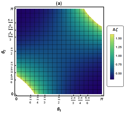
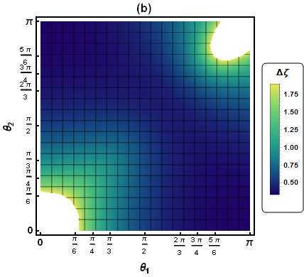
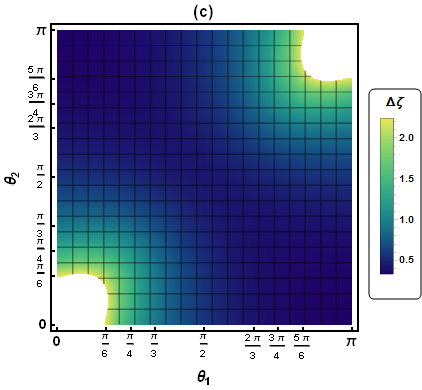
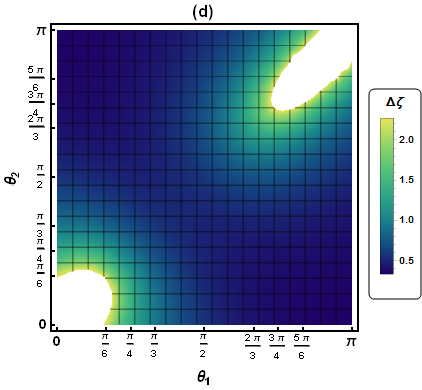
Figure 1: Density of the Cramer-Rao bound $\Delta{\zeta}_{\Phi}^{S_{z}}$ versus $\theta_{1}$ and $\theta_{2}$ with $\varphi_{1}=0$. Fig.(a) is obtained for $\varphi_{2}=0$. Fig.(b) is for $\varphi_{2}=\pi/2$. Fig.(c) is for $\varphi_{2}=4\pi/3$ and Fig.(d) is for $\varphi_{2}=\pi$.

In Figure 1($b$), we display the behavior of $\Delta{\zeta}_{\Phi}^{S_{z}}$ versus $\theta_{1}$ and $\theta_{2}$ with ${\Phi=\frac{\pi}{2}}$ (see the appendix A). When $\Phi=\frac{\pi}{2}$, the best performance is achieved for $\theta_{1}=0$ and $\theta_{2}=\pi$ or vice versa. By contrast, the quantum Cramer-Rao bound diverges for $\theta_{1}=\theta_{2}=0$ and $\theta_{1}=\theta_{2}=\pi$. The other interesting situation would be to consider $\Delta{\zeta}$ along the line $\theta_{2}={\pi}-\theta_{1}$. In this case, the value of quantum Cramer-Rao bound is between the Heisenberg limit and the standard quantum limit.

In Figure 1($c$), we examine the performance of the density $\Delta{\zeta}$ with ${\Phi=\frac{4\pi}{3}}$ (in this scenario, the analytical expression for the quantum Cramer-Rao bound is given in the appendix A). The density $\Delta{\zeta}$ exhibits symmetry with respect to $\theta_{1}$ and $\theta_{2}$. Notably, when one of these angles is set to $0$ and the other to $\pi$, the state achieves Heisenberg limit sensitivity, resulting in $\Delta{\zeta}=1/3$. Hence, $\Delta{\zeta}=0.4236$ holds for $\theta_{1}=\theta_{2}$, while it deviates for $\theta_{1}=0,\pi$. Another intriguing scenario involves considering $\Delta{\zeta}_{\Phi=\frac{4\pi}{3}}^{S_{z}}$ along the line $\theta_{1}=\pi-\theta_{2}$. In this instance, the Cramer-Rao bound assumes values within the range of Heisenberg limit and standard quantum limit (i.e. ${\rm HL}\leq\Delta{\zeta}_{\Phi=\frac{4\pi}{3}}^{S_{z}}\leq{\rm SQL}$).

Finally, when we set $\Phi=\varphi_{1}-\varphi_{2}={\pi}$ as depicted in Figure 1($d$) (see the appendix A), the Cramer-Rao bound reached the Heisenberg limit when $\theta_{1}=0$ and $\theta_{2}=\pi$ or vice versa. Conversely, it diverges for $\theta_{1}=\theta_{2}=0$ and $\theta_{1}=\theta_{2}=\pi$. The other interesting scenario would be to consider $\Delta{\zeta}$ along the line $\theta_{2}=\pi-\theta_{1}$. As a result, the Cramer-Rao bound takes values between the Heisenberg limit and the standard quantum limit. As a consequence, in all these plots, where $\theta_{1}=0$, $\theta_{2}=\pi$ or else $\theta_{1}=\pi$, $\theta_{2}=0$, the phase estimate is optimal. This phenomenon arises due to the fact that, in these instances, the cat state represents a superposition of two antipodal states on the Bloch sphere. Indeed, the superposition of spin coherent states situated antipodally on the Bloch sphere exhibits behaviors akin to NOON states within quantum metrology [46]. Thus, the explicit expression of the cat state is reduced to

$$|Cat,3/2\rangle=N(|\theta_{1},\varphi,3/2\rangle+|\pi-\theta_{1},\varphi,3/2\rangle),$$ (23)

where, in this scenario, $\varphi_{1}$ and $\varphi_{2}$ lose their significance at the poles, resulting in phase sensitivity becoming independent of them. Based on the above results, we deduce that the Heisenberg limit is inversely proportional to the $s$-spin according to the relationship $\Delta\zeta_{HL}=1/2s$.

III.2 Quantum metrological performance of $3/2$-spin cat states under the influence of generator $S_{x}$

In this second scenario, we examine the metrological performance of $3/2$-spin cat states that accumulates a phase through $e^{i{\zeta}S_{x}}$. The analytical expression for the quantum Cramer–Rao bound is given by

$$\Delta{\zeta}^{S_{x}}=\Bigr{[}{3N_{c}^{2}{(A^{2}+D\bar{D}+7B\bar{B}+7C\bar{C}+2AC+2A\bar{C}+2B\bar{D}+2D\bar{B})}-{9N_{c}^{4}(AB+A\bar{B}+2C\bar{B}+2B\bar{C}+C\bar{D}+D\bar{C})^{2}}}\Bigr{]}^{\frac{-1}{2}},$$ (24)

The general expression of $\Delta{\zeta}^{S_{x}}$ is contingent upon $\varphi_{1}$, $\varphi_{2}$, $\theta_{1}$ and $\theta_{2}$. Consequently, by fixing $\varphi_{1}$ at $0$, we plot $\Delta{\zeta}^{S_{x}}$ in terms of $\theta_{1}$ and $\theta_{2}$ for various values of $\varphi_{2}$, aiming to identify cases of enhanced accuracy. Accordingly, based on the outcomes depicted in Figure (2), optimal precision is achieved when $\Delta{\zeta}^{S_{x}}$ lies within or equates the range between the standard and Heisenberg quantum limits.

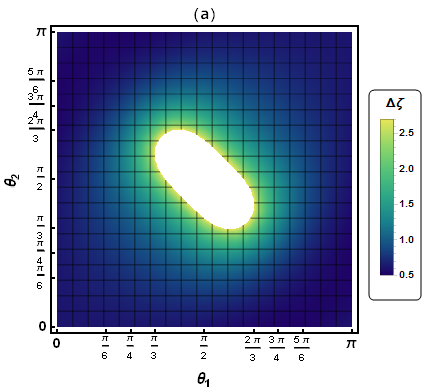
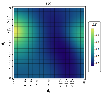
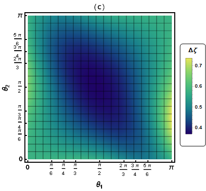
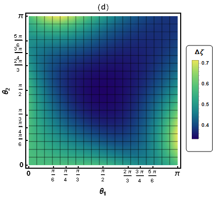
Figure 2: Density of the Cramer-Rao bound $\Delta{\zeta}_{\Phi}^{S_{x}}$ versus $\theta_{1}$, $\theta_{2}$ and ${\Phi}=\varphi_{1}-\varphi_{2}$ with $\varphi_{1}=0$. Fig.(a) is obtained for $\varphi_{2}=0$. Fig.(b) is for $\varphi_{2}=\pi/2$. Fig.(c) is for $\varphi_{2}=3\pi/4$ and Fig.(d) is for $\varphi_{2}=\pi$.

In Figure 2($a$), we have explored the scenario with $\varphi_{2}=0$, resulting in minimal $\Delta{\zeta}^{S_{x}}$ values occurring at $\theta_{1}=\theta_{2}=0,\pi$, with $\Delta{\zeta}^{S_{x}}=0.577$. On the other hand, the highest value of $\Delta{\zeta}^{S_{x}}$ is observed for $\theta_{2}=\pi-\theta_{1}$ within the region of $\frac{\pi}{3}\leq\theta_{2}\leq{\frac{2\pi}{3}}$. In the second case (Fig. 2(b)) with ${\varphi_{2}}=\frac{\pi}{2}$, $\Delta{\zeta}^{S_{x}}$ reaches an optimum within the dark blue-shaded region, approximately at the value of $0.4$. For instance, at $\theta_{1}=0$ and $\theta_{1}=\frac{3\pi}{4}$, $\Delta{\zeta}^{S_{x}}=0.479$.

The behavior of quantum Cramer-Rao bound as a function of $\theta_{1}$ and $\theta_{2}$, with $\Phi=\frac{3\pi}{4}$ is illustrated in Figure 2($c$). Based on this outcome, it is evident that the estimation is most precise in the region where $\theta_{1}=\theta_{2}=\frac{\pi}{2}$, as the phase measurement error approaches approximately $0.3693$. Furthermore, there exist regions in which $\Delta{\zeta}^{S_{x}}$ provides a better sensitivity: $\frac{\pi}{3}\leq{\theta_{1}}\leq{\frac{3\pi}{4}}$ and $\frac{\pi}{3}\leq{\theta_{2}}\leq{\frac{3\pi}{4}}$. For instance, by selecting $\theta_{1}=\frac{2\pi}{3}$ and $\theta_{1}=\frac{\pi}{3}$, we obtain $\Delta{\zeta}^{S_{x}}\simeq{0.3985}$.

The identical plot with $\varphi_{2}=\pi$ is depicted in Figure 2(d). Consequently, $\Delta{\zeta}^{S_{x}}$ is optimized within the region where $\frac{\pi}{3}\leq\theta_{1}=\theta_{2}\leq\frac{5\pi}{6}$. Another noteworthy scenario in this context involves considering $\theta_{2}=\pi-\theta_{1}$. From Figure 2(d) , we can see that $\Delta{\zeta}^{S_{x}}$ provides a better sensitivity along this line in the region where $\frac{\pi}{3}\leq\theta_{1}=\theta_{2}\leq\frac{2\pi}{3}$. While, if $\theta_{1}=\theta_{2}=\frac{\pi}{2}$, we immediately attain the Heisenberg limit sensitivity (see the appendix B).

III.3 Quantum metrological performance of $3/2$-spin cat states with the parameter-generating operator $S_{y}$

Finally, we will explore the scenario in which the system accumulates a phase through $e^{i\zeta{S_{y}}}$. Employing a similar approach as described earlier, the Cramer–Rao bound reduces to

$$\Delta{\zeta}^{S_{y}}=\Bigr{[}{3N_{c}^{2}{(A^{2}+D\bar{D}+7B\bar{B}+7C\bar{C}-2AC-2A\bar{C}-2B\bar{D}-2D\bar{B})}+{9N_{c}^{4}(AB-A\bar{B}+2C\bar{B}-2B\bar{C}-C\bar{D}+D\bar{C})^{2}}}\Bigr{]}^{\frac{-1}{2}},$$ (25)

and the associated ultimate parameter estimation limit, for the phase difference $\Phi=0$ and $\Phi=\frac{\pi}{2}$, are given by

$$\Delta{\zeta}_{\Phi=0}^{S_{y}}=\frac{1}{\sqrt{9-\frac{12}{3-2\cos{\left(\frac{\theta_{1}-\theta_{2}}{2}\right)+\cos{\left(\theta_{1}-\theta_{2}\right)}}}}},\hskip 42.67912pt\Delta{\zeta}_{\Phi=\frac{\pi}{2}}^{S_{y}}=\frac{2\sqrt{2}[-2+\Sigma\cos(\frac{\theta_{1}}{2})\cos(\frac{\theta_{2}}{2})]}{\sqrt{3\Bigr{[}{\varPi+\Upsilon+\Omega-\Lambda+36}\Bigr{]}}},$$ (26)

where

$$\Sigma=1+\cos(\theta_{1})\Bigl{[}-2+\cos(\theta_{2})\Bigl{]}-2\cos(\theta_{2}),\hskip 28.45274pt\varPi=8\cos(\theta_{1})\cos^{2}(\theta_{2})+4\cos(2\theta_{1})\Bigl{[}1+3\cos^{2}{(\frac{\theta_{1}}{2})}\cos^{3}({\theta_{2}})\Bigl{]},$$

$$\Upsilon=\cos^{2}{(\frac{\theta_{1}}{2})}\Bigl{\{}\cos(\theta_{2})\Bigr{[}13-16\cos(\theta_{1})\cos(2\theta_{2})\Bigr{]}+7\cos(3\theta_{2})\Bigl{\}},\hskip 28.45274pt\Lambda=8\sin^{2}{(\theta_{1})}\cos(2\theta_{2}),$$

$$\Omega=2\cos(\frac{\theta_{1}}{2})\Bigl{\{}2\cos(\frac{\theta_{2}}{2})\Bigl{[}-3+\cos(\theta_{1})\Bigl{(}18-5\cos(\theta_{2})+2\cos(2\theta_{2})+\cos(3\theta_{2})\Bigl{)}\Bigl{]}+8\cos(\frac{3\theta_{2}}{2})-2\cos(\frac{7\theta_{2}}{2})\Bigl{\}},$$ (27)

and for $\Phi=\frac{\pi}{3}$ and $\Phi=\pi$ are

$$\Delta{\zeta}_{\Phi=\frac{\pi}{3}}^{S_{y}}=\frac{32+\Sigma^{{}^{\prime}}}{\sqrt{3\Bigr{[}\varPi^{{}^{\prime}}(32+\Sigma^{{}^{\prime}})+(-1)^{\frac{2}{3}}12\Upsilon^{{}^{\prime}}\Bigr{]}}},\hskip 56.9055pt\Delta{\zeta}_{\Phi=\pi}^{S_{y}}=\Delta{\zeta}_{\Phi=0}^{S_{y}},$$ (28)

where

$$\begin{split}\Sigma^{{}^{\prime}}&=9\cos\bigl{(}\frac{\theta_{1}-3\theta_{2}}{2}\bigl{)}+9\cos\bigl{(}\frac{3\theta_{1}-\theta_{2}}{2}\bigl{)}+15\cos\bigl{(}\frac{\theta_{1}+\theta_{2}}{2}\bigl{)}-\cos\bigl{(}\frac{3\theta_{1}+3\theta_{2}}{2}\bigl{)},\\ \varPi^{{}^{\prime}}&=44+3\cos\bigl{(}\frac{\theta_{1}-3\theta_{2}}{2}\bigl{)}+27\cos\bigl{(}\frac{3\theta_{1}-\theta_{2}}{2}\bigl{)}-12\cos(2\theta_{2})+5\cos\bigl{(}\frac{\theta_{1}+\theta_{2}}{2}\bigl{)}-3\cos\bigl{(}\frac{3\theta_{1}+\theta_{2}}{2}\bigl{)},\\ \Upsilon^{{}^{\prime}}&=[1+(-1)^{\frac{1}{3}}]^{2}\sin^{2}\bigl{(}{\frac{\theta_{2}}{2}}\bigl{)}\Bigr{[}{\cos\bigl{(}\frac{\theta_{1}}{2}\bigl{)}+3\cos\bigl{(}\frac{3\theta_{1}}{2}\bigl{)}+3\cos\bigl{(}\frac{3\theta_{1}}{2}-\theta_{2}\bigl{)}+8\cos\bigl{(}\frac{\theta_{2}}{2}\bigl{)}+\cos\bigl{(}\frac{\theta_{1}}{2}+\theta_{2}\bigl{)}}\Bigr{]}^{2}.\end{split}$$ (29)

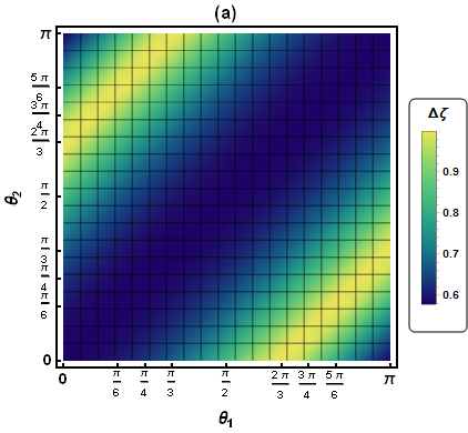
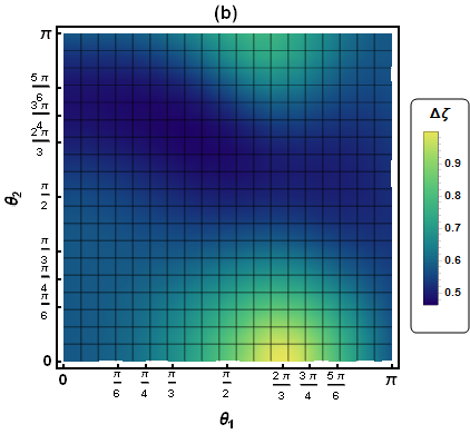
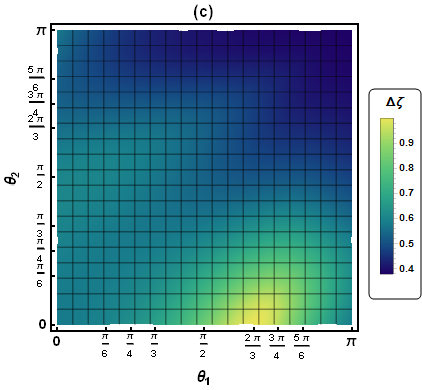
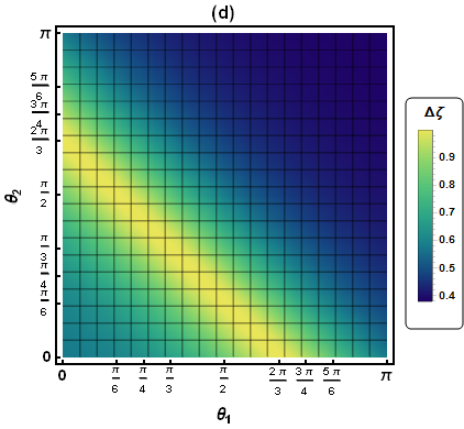
Figure 3: Density of the Cramer-Rao bound $\Delta{\zeta}_{\Phi}^{S_{y}}$ versus $\theta_{1}$, $\theta_{2}$ and ${\Phi}=\varphi_{1}-\varphi_{2}$ with $\varphi_{1}=0$. Fig.(a) is obtained for $\varphi_{2}=0$. Fig.(b) is for $\varphi_{2}=\pi/2$. Fig.(c) is for $\varphi_{2}=\pi/3$ and Fig.(d) is for $\varphi_{2}=\pi$.

From Figure 3($a$), it is evident that the minimum sensitivity occurs when $\theta_{1}=\theta_{2}$, which corresponds to the standard quantum limit. Moreover, the same sensitivity is obtained for cases where $\theta_{1}=0$ and $\theta_{2}=\pi$ or $\theta_{1}=\pi$ and $\theta_{2}=0$. Moving to the second scenario (depicted in Figure 3($b$)), $\Delta{\zeta}^{S_{y}}$ reaches its minimum when $\theta_{1}=0$ and $\theta_{2}=\pi$ or $\theta_{1}=\pi$ and $\theta_{2}=0$, resulting in $\Delta{\zeta}^{S_{y}}=0.471$, a value between the standard quantum limit and the Heisenberg limit. Furthermore, the density Cramer–Rao bound falls below the quantum standard limit within certain regions, such as $0\leq\theta_{1}\leq{\frac{5\pi}{6}}$ and ${\frac{2\pi}{3}}\leq\theta_{2}\leq{\frac{5\pi}{6}}$ simultaneously. As an illustration, for $\theta_{1}=\pi/6$ and $\theta_{2}=5\pi/6$, the density $\Delta{\zeta}^{S_{y}}$ is approximately $0.361$. In the case where $\Phi=\frac{\pi}{3}$ (depicted in Figure 3($c$)), the density Cramer–Rao bound offers improved sensitivity when $\theta_{1}=\theta_{2}=\pi$, as well as in the region surrounding this point. Finally, considering $\Phi=0$ (refer to Figure 3($d$)), we find that $\Delta{\zeta}^{S_{y}}$ equals $0.377964$ when $\theta_{1}=\theta_{2}=\pi$. Clearly, this value approaches the Heisenberg limit $1/3$.

IV Quantum phase estimations via $s$-spin cat states

Here, we present a comprehensive analytical expression for the quantum Fisher information, facilitating the computation of the Cramer-Rao bound for an unknown parameter within the coherent states superposition of any spin $s$. To investigate the metrological power of a generic superposition of spin coherent states, we derive a general formulation of the QFI for situations where the system accumulates phases via $e^{i\zeta{S}_{x}}$, $e^{i\zeta{S}_{y}}$ and $e^{i\zeta{S}_{z}}$. Notably, we aim to ascertain the precision limitations in each scenario. To achieve this objective, we consider that the states described by (8) can be alternatively expressed in a more general form as [47, 48, 49, 50]

$$\begin{split}|\theta,\varphi,s\rangle&=\left(1+|z|^{2}\right)^{-s}\sum_{m=-s}^{s}{\binom{2s}{s+m}}^{\frac{1}{2}}{z}^{s+m}|s,m\rangle,\end{split}$$ (30)

where $z=e^{-i\varphi}\tan{(\frac{\theta}{2})}$ and the overlap of two SCSs is

$$\begin{split}\langle{\theta_{1},\varphi_{1},s}|\theta_{2},\varphi_{2},s\rangle&=\frac{(1+\bar{z_{1}}z_{2})^{2s}}{(1+|z_{1}|^{2})^{s}(1+|z_{2}|^{2})^{s}},\end{split}$$ (31)

here, $z_{1}=e^{-i\varphi_{1}}\tan{(\frac{\theta_{1}}{2})}$ and $z_{2}=e^{-i\varphi_{2}}\tan{(\frac{\theta_{2}}{2})}$. Therefore, the general form of the superposition of two spin coherent states could be written as

$$\begin{split}|cat,s\rangle&={\cal N}_{c}\left(|\theta_{1},\varphi_{1},s\rangle+|\theta_{2},\varphi_{2},s\rangle\right),\\ &={\cal N}_{c}\sum_{m=-s}^{s}{\binom{2s}{s+m}}^{\frac{1}{2}}\left[{\frac{{z_{1}}^{s+m}}{(1+|z_{1}|^{2})^{s}}+\frac{{z_{2}}^{s+m}}{(1+|z_{2}|^{2})^{s}}}\right]|s,m\rangle,\end{split}$$ (32)

in termes of $z_{1},z_{2}$, and the normalization factor ${\cal N}_{c}$ given by

$${\cal N}_{c}=\left[{2+\frac{(1+\bar{z_{1}}z_{2})^{2s}+(1+\bar{z_{2}}z_{1})^{2s}}{(1+|z_{1}|^{2})^{s}(1+|z_{2}|^{2})^{s}}}\right]^{\frac{-1}{2}}.$$ (33)

The analytical expressions of the quantum Fisher information for $s$-spin coherent states, in three parameter-generating operators $H=S_{z}$, $H=S_{x}$ and $H=S_{y}$, are proved in appendix C. In the following, we illustrate the behavior of the quantity $\Delta\zeta$ when the dynamics of the generalized state (30) is governed by the spin operators $S_{x}$, $S_{y}$, and $S_{z}$. It is noteworthy that in Figures 4 and 5, we have taken $\theta=\theta_{1}=\theta_{2}\in[0,\pi]$. For the other figures, specifically Fig.6, Fig.7 and Fig.8, we have kept $\theta_{2}$ fixed ($\theta_{2}=\frac{\pi}{2}$) while allowing $\theta_{1}$ to vary within the range $[0,\pi]$ for all three cases.

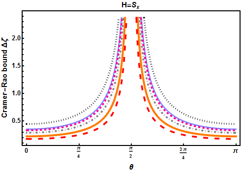
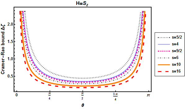
Figure 4: Density of the Cramer-Rao bound versus $\theta$ for different values of $s$, with ${\Phi}$=$\varphi_{1}-\varphi_{2}=0$.

Figure 4 depicts the Cramer-Rao bound plotted against $\theta$ for $\Phi=\phi_{1}-\phi_{2}=0$ and various spin values. When undergoing a unitary evolution along the $x$-direction $(i.e.H=S_{x})$, the Cramer-Rao bound exhibits a minimum within the intervals $[0,\pi/4]$ and $[3\pi/4,\pi]$. If $\theta$ take the values 0 and $\pi$, the Cramer-Rao bound attains the standard quantum limit. For instance, $\Delta{\zeta}=0.44$ for $s=5/2$, $\Delta{\zeta}=0.35$ for $s=4$ and $\Delta{\zeta}=0.33$ for $s=9/2$ and so forth. Furthermore, the Cramer-Rao bound rises to a maximum value within the ranges $\theta\in[\pi/4,\pi/2[$ and $\theta\in]\pi/2,3\pi/4]$, while it diverges at $\theta=\pi/2$. When experiencing a unitary evolution along the $y$-direction $(i.e.H=S_{y})$, the Cramer-Rao bound density maintains a constant value for each spin, which aligns with the standard quantum limit. Conversely, in the case of a unitary evolution along the $z$-direction $(i.e.H=S_{z})$, maximum precision is achieved for each spin when $\theta=\pi/2$.

Based on the outcomes, we observe a consistent pattern in the Cramer-Rao bound density resembling that of a spin $3/2$ across all three directions, with only the Heisenberg limit changing when $s$ changes. Moreover, the figures unmistakably illustrate that the estimation with $S_{y}$ is better, as Cramer-Rao bound remains stable for various values of $s$. Nevertheless, in scenarios where $H=S_{x}$ and $H=S_{z}$, $\Delta{\zeta}$ diverges at $\theta=\pi/2$ and $\theta=0,\pi$, respectively.

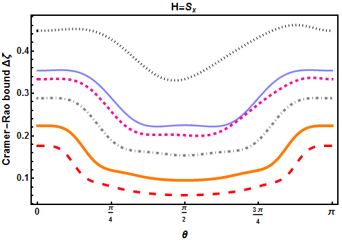
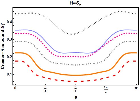
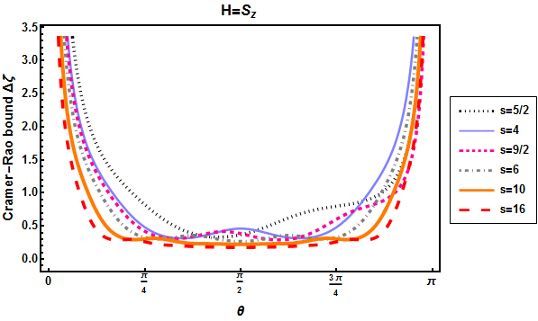
Figure 5: Density of the Cramer-Rao bound versus $\theta$ for different values of s. ${\Phi}$=$\varphi_{1}-\varphi_{2}$=$\pi/2$ in these plots.

Figure (5) presents similar plots, but this time, we consider ${\Phi}=\varphi_{1}-\varphi_{2}=\pi/2$. It is easily seen that the density of the Cramer-Rao bound $\Delta{\zeta}$ behaves along the $x$-direction in a manner akin to its behavior along the $y$-direction. In this scenario, the highest accuracy is attained when $\theta$ falls within the interval $[\pi/4,3\pi/4]$. However, in the case of the $z$-direction, the Cramer-Rao bound density is minimum when $\theta=\pi/2$ for $s=16,10,6$. While, the minimum sensitivity happens for $\theta=\pi/3,3\pi/4$ when $s=4$ yielding $\Delta{\zeta}\approx{0.32}$. When considering $s=5/2$, the density of Cramer-Rao bound is maximal for ${\theta}\in{]{\pi/3,\pi/2}[}$ and it gives $\Delta{\zeta}\approx{0.34}$. Finally, in the case of $s=9/2$, $\Delta{\zeta}$ provides a better sensitivity when ${\theta}\in[{\pi/4,\pi/3}]$ and ${\theta}\in]\pi/2,2\pi/3[$, then $\Delta{\zeta}=0.3$ and $\Delta{\zeta}=0.28$ respectively.

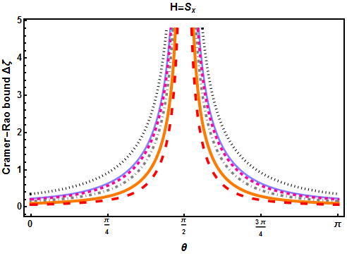
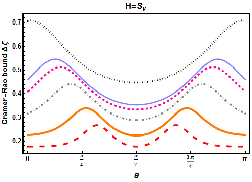
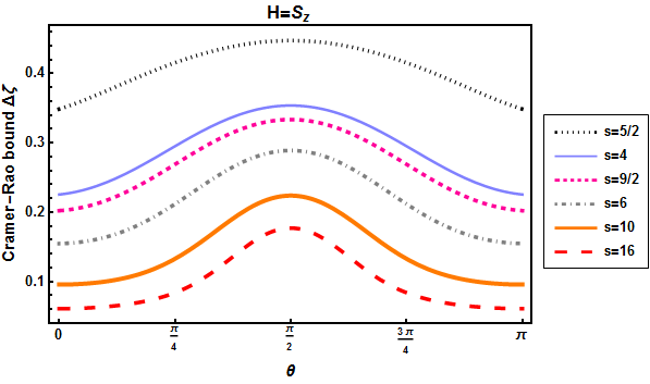
Figure 6: Density of the Cramer-Rao bound versus $\theta$ for different values of $s$, with ${\Phi}=0$, $\theta=\theta_{1}$ and $\theta_{2}=\pi/2$.

Notably, in Figures (6), it is striking to observe that the Cramer-Rao bound density under the influence of the Hamiltonian $H=S_{x}$ attains its minimum at $\theta=0,\pi$, with $\Delta\zeta$ values falling between the Heisenberg Limit and the Standard Quantum Limit for the various chosen spin values. However, at $\theta=\pi/2$, $\Delta\zeta$ diverges. For the case of $H=S_{y}$, the Cramer-Rao bound density exhibits a noticeable minimum when $\theta=\pi/2$ across the specified spin values. Nonetheless, when $\theta=0,\pi$, $\Delta{\zeta}$ reaches a minimum solely for $s=4,9/2,6,10,16$. By contrast, the density of the Cramer-Rao bound when the Hamiltonian $H=S_{z}$ is optimal where $\theta=0,\pi$ for differents values of $s$-spin, and $\Delta{\zeta}$ is between SQL and HL. For instance, considering the case of spin $s=4$, we have ${\rm SQL}=0.44\leq{\Delta{\zeta}}\approx{0.35}\leq{\rm HL}=0.2$. This outcome parallels the results for other $s$-spin values.

However, the situation is slightly different for ${\Phi}=\pi$ (see Fig.7). When the input state evolves along the $x$-direction $(H=S_{x})$, the phase estimation becomes minimal in the interval $\theta{\in}[{\pi/4,3\pi/4}]$ and especially for $\theta=\pi/2$. In the situation where $H=S_{y}$, the function $\Delta{\zeta}$ decreases to attain the minimum values at an angle $\theta=\pi$ for half-integer values of spin $s=5/2$ and $s=9/5$, but it’s different for the integer spin $s=4,6,10,16$. On the one hand, we can see from figure, that after an initial decreasing, the density of Cramer-Rao bound increases for $s=4,6$ and the best estimation of the phase shift parameter is achieved for $\theta=\pi/2$. On the other hand, for $s=10,16$, the value of $\Delta{\zeta}$ remains constant in the interval $[0,\pi]$ and lies between SQL and HL. Finally, in the case where $H=S_{z}$, the best accuracy is obtained when $\theta=0$ or $\theta=\pi$.

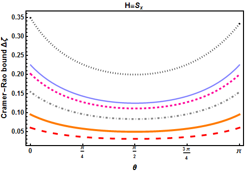
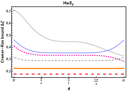
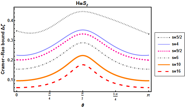
Figure 7: Density of the Cramer-Rao bound versus $\theta$ for different values of $s$ with ${\Phi}=\pi$, $\theta=\theta_{1}$ and $\theta_{2}=\pi/2$.

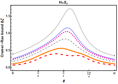
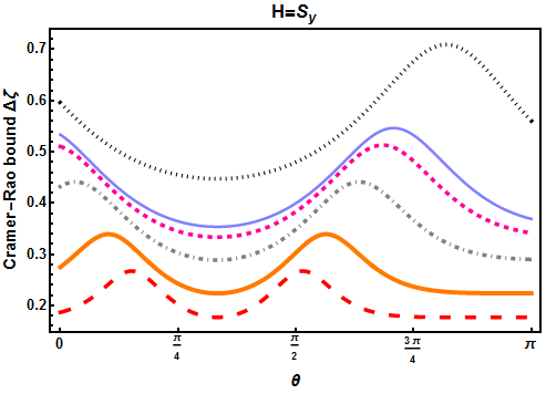
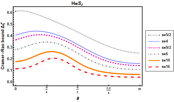
Figure 8: Density of the Cramer-Rao bound versus $\theta$ for different values of $s$ with ${\Phi}=0$, $\theta=\theta_{1}$ and $\theta_{2}=\pi/3$.

Figures 8 depict the Cramer-Rao bound as a function of $\theta$ for various $s$ values with ${\Phi}=0$, $\theta=\theta_{1}$, and $\theta_{2}=\pi/3$. It is evident that, for $H=S_{x}$, the behavior of the Cramer-Rao bound is similar of that seen in 6 and we again observe a minimum value of $\Delta{\zeta}$ at angles $\theta=0,\pi$ for different $s$ values, along with a maximum value at $\theta=0,\pi/2$. When considering a unitary evolution along the y-direction $(H=S_{y})$, the Cramer-Rao bound attains its minimum at approximately the midpoint of the interval $[\pi/4,\pi/2]$, as well as at $\theta=\pi$, for various $s$ values. Now, let us turn our attention to the case where $H=S_{z}$. The optimal estimation is achieved when $\theta=\pi$, and even when $\theta$ is in close proximity to $\pi$, across different $s$ values.

In Figures (9), (10), and (11), we have graphed the CRB density as a function of $\theta_{1}$ and $\theta_{2}$ for the x-direction ($H=S_{x}$), y-direction ($H=S_{y}$), and z-direction ($H=S_{Z}$), respectively. These plots consider phase differences $\Phi=\varphi_{1}-\varphi_{2}=0,\pi/2$, and $\Phi=\pi$. The primary aim of these plots is to compare the behavior of the density $\Delta{\zeta}$ for different $s$ values (specifically $s=5/2,4,9/2,16$) with the earlier results obtained for spin $s=3/2$ and to examine how $\Delta{\zeta}$ evolves with increasing $s$. Furthermore, these plots are designed to illustrate scenarios where the Cramer-Rao bound approaches the Heisenberg limit.

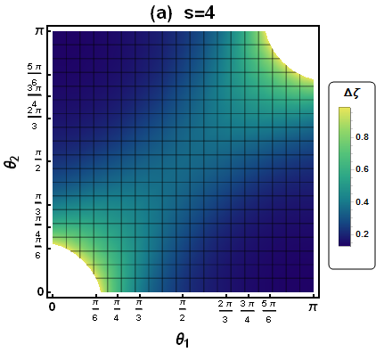
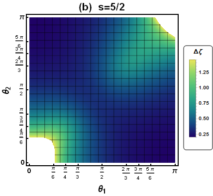
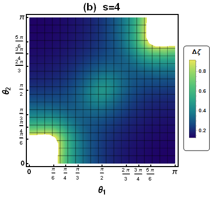
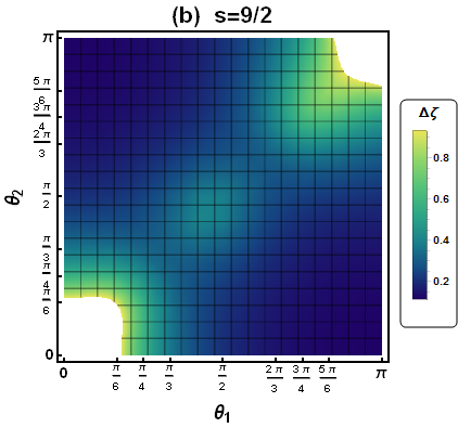
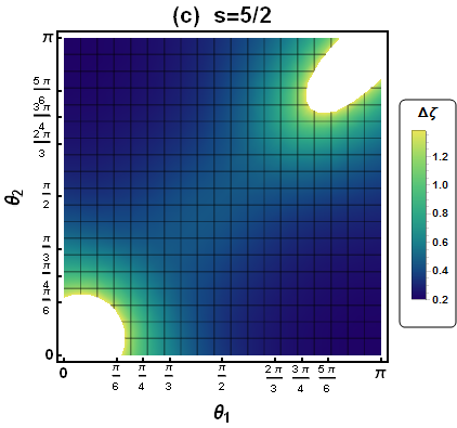
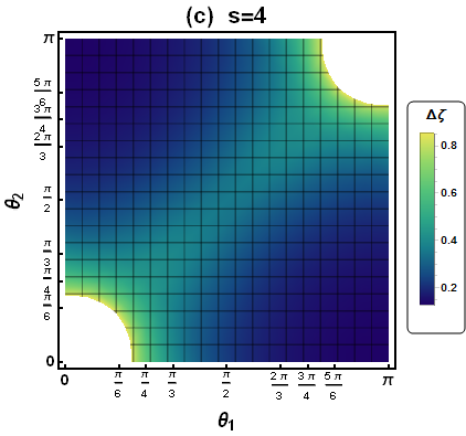
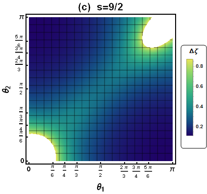
Figure 9: Density of the Cramer-Rao bound versus $\theta_{1}$ and $\theta_{2}$ for different values of $s$ when $H=J_{z}$. Fig.(a) is for ${\Phi}=0$, Fig.(b) is for ${\Phi}=\pi/2$, and Fig.(c) is for ${\Phi}=\pi$.

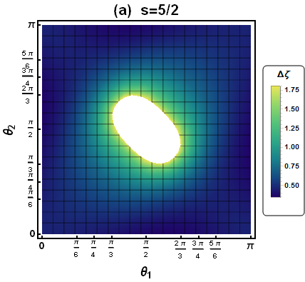
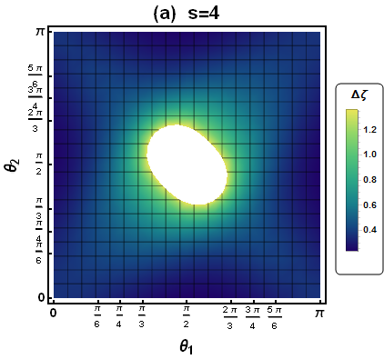
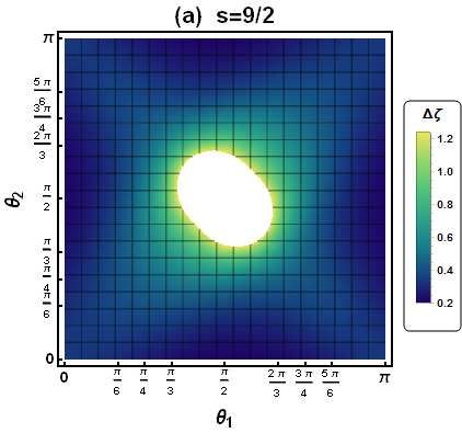
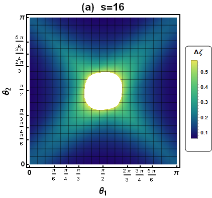
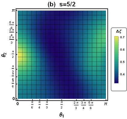
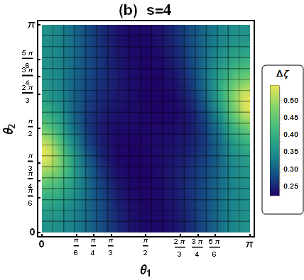
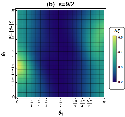
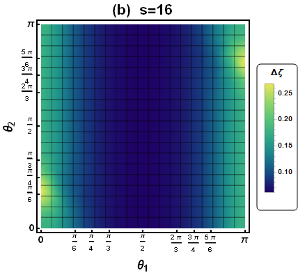
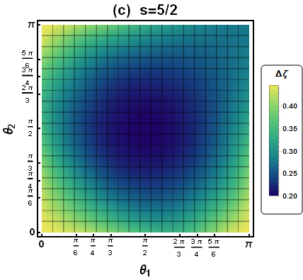
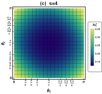
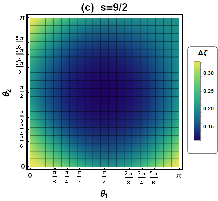
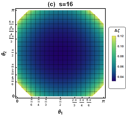
Figure 10: Density of the Cramer-Rao bound versus $\theta_{1}$ and $\theta_{2}$ for different values of $s$ when $H=J_{x}$. Fig.(a) is for ${\Phi}=0$, Fig.(b) for ${\Phi}$=$\pi/2$, and Fig.(c) is for ${\Phi}$=$\pi$.

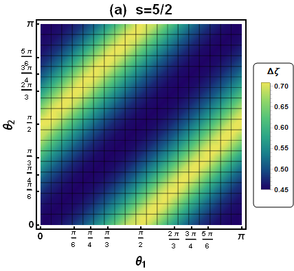
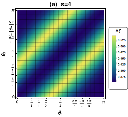
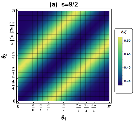
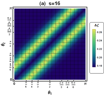
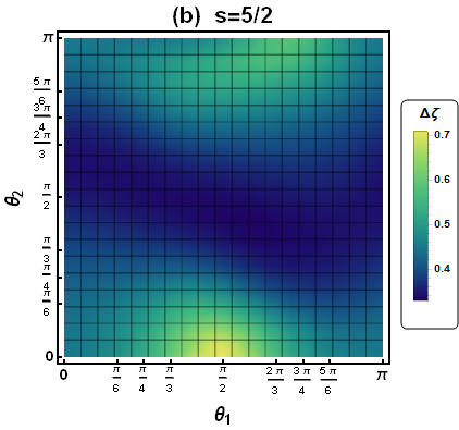
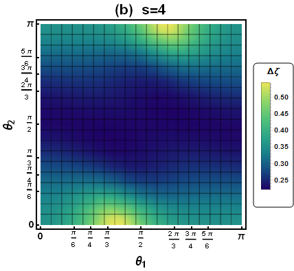
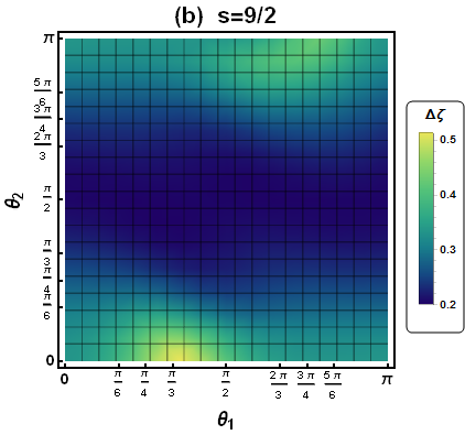
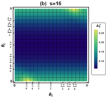
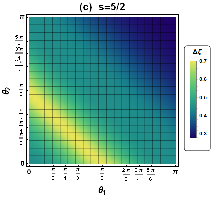
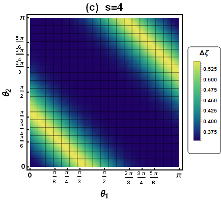
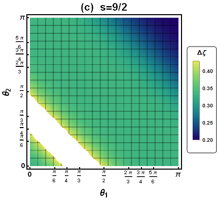
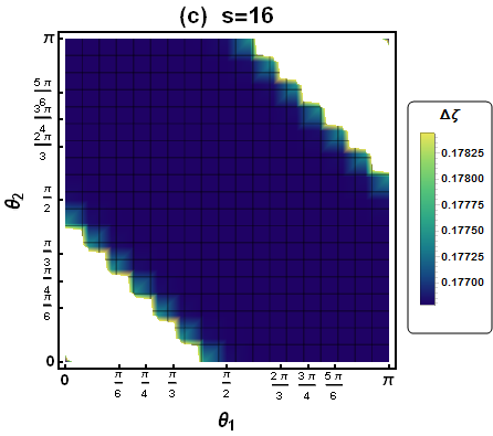
Figure 11: Density of the Cramer-Rao bound versus $\theta_{1}$ and $\theta_{2}$ for different values of $s$ when $H=J_{y}$. Fig.(a) is for ${\Phi}=0$, Fig.(b) is for ${\Phi}$=$\pi/2$, and Fig.(c) is for ${\Phi}$=$\pi$.

To begin with, when comparing the density shapes obtained for different values of $s$ with the previous graphs of $s=3/2$, we observe similar shapes but with varying values and Heisenberg limits as s changes. Clearly, for $H=S_{z}$ (Fig.9), the density $\Delta\zeta$ diverges at $\theta_{1}=\theta_{2}=0$ or $\theta_{1}$=$\theta_{2}=\pi$, but is optimal at $\theta_{1}=0$ and $\theta_{2}=\pi$, or vice versa. This is due to the superposition of two antipodal states on the Bloch sphere, resulting in NOON states that exhibit Heisenberg limit precision. Secondly, in the case where $H=S_{x}$ and $\Phi=0$ (Fig.10($a$)), the Cramer-Rao bound diverges around and into the point $\theta_{1}=\theta_{2}=\frac{\pi}{2}$. Furthermore, the density $\Delta{\zeta}$ is between the quantum standard limit and the Heisenberg limit when ($\theta_{1}=0,\pi$ and $0<\theta_{2}<\pi$) or ($0<\theta_{1}<\pi$ and $\theta_{2}=0,\pi$). For $\Phi=\frac{\pi}{2}$, the Cramer-Rao bound is minimal when ($\frac{\pi}{3}<\theta_{1}<\frac{2\pi}{3}$) for $s=5/2$, and the interval expands as s increases (Fig.12($b$)). We set $\Phi=\pi$ in Fig.12($c$). In this case, the estimation is more accurate at the point $\theta_{1}=\theta_{2}=\frac{\pi}{2}$. Finally, when $H=J_{y}$ and $\Phi=0$ (Fig.11($a$)), the minimum sensitivity occurs when $\theta_{1}=\theta_{2}$, as well as when ($\theta_{1}=0$ and $\theta_{2}=\pi$) or ($\theta_{1}=\pi$ and $\theta_{2}=0$). In the second case, when $\Phi=\frac{\pi}{2}$ (Fig.11($b$)), the CRB is minimal when ($\frac{\pi}{3}<\theta_{2}<\frac{2\pi}{3}$) for $s=5/2$, and the interval expands as s increases. In figures 13($c$), we take $\Phi=\pi$. The density $\Delta{\zeta}$ approaches the Heisenberg limit when $\theta_{1}=\theta_{2}=\pi$. On the other hand, if the spin s is an integer (for example $s=4$ and $s=16$), the density is also minimal in the region where $\theta_{1}=\pi-\theta_{2}$. As $s$ increases in the integer case, the density increases in the regions where $\theta_{1}=\theta_{2}=0,\pi$, and then becomes divergent in the larger values of $s$ (for example $s=16$).

In summary, the minimum value of the Cramer-Rao bound typically falls within the range situated between the Heisenberg limit and the standard quantum limit across various scenarios. It attains the Heisenberg limit under specific conditions contingent upon judiciously chosen parameters $\theta_{1}$, $\theta_{2}$, and the phase difference $\Phi=\varphi_{1}-\varphi_{2}$. Moreover, drawing from preceding findings, it becomes evident that the most precise estimation emerges when $H=S_{z}$, particularly when $\theta_{1}=0$ and $\theta_{2}=\pi$ (or equivalently $\theta_{1}=\pi$ and $\theta_{2}=0$), thereby optimizing the Cramer-Rao bound. This behavior arises from the antipodal nature of the superposed states on the Bloch sphere. Indeed, such superposed spin coherent states, positioned antipodally on the Bloch sphere, exhibit analogous behavior to NOON states within the realm of quantum metrology. However, in instances where $H=S_{x}$ and $H=S_{y}$, the Cramer-Rao bound frequently aligns with the standard quantum limit or resides within the range between the standard quantum limit and the Heisenberg limit. Sometimes, there exist select cases where the Cramer-Rao bound reaches the Heisenberg limit.

V Closing remarks

In conclusion, we have thoroughly investigated the metrological performance of superposed $3/2$-spin coherent states and derived an explicit expression for the quantum Cramer-Rao bound specific to this spin configuration. Subsequently, we scrutinized the outcomes for each scenario involving the parameter-generating operator $H$ while considering the Heisenberg limit. To exemplify our study, we derived a general formulation for the quantum Fisher information pertaining to the superposition of $s$-spin coherent states when $H=S_{x}$, $H=S_{y}$, $H=S_{z}$. We presented Cramer-Rao bound plots for each case, showcasing diverse $s$ values. Our investigation reveals that the Heisenberg limit decreases with an increase in the spin number, and this decrease is inversely proportional to $s$, as denoted by the relationship $\Delta\zeta_{\rm HL}=\frac{1}{2s}$. As an example, when $s=1$, ${\rm HL}=0.5$; for $s=3/2$, ${\rm HL}=1/3$; and for $s=4$, ${\rm HL}=0.125$, and so forth. Moreover, our study underscores the profound influence of the chosen parameter-generating operator on quantum metrology and its pivotal role in determining the precision of an unknown parameter. Based on our comprehensive findings, it becomes evident that the operator $S_{z}$ leads to the most accurate estimations, and with this operator, we reach the Heisenberg limit, resulting in optimal phase estimates. This is because the cat state represents a superposition of two antipodal states on the Bloch sphere ($\theta_{1}=0$, $\theta_{2}=\pi$, or $\theta_{1}=\pi$, $\theta_{2}=0$). Indeed, the superposition of spin coherent states located antipodally on the Bloch sphere exhibits behaviour similar to NOON states in quantum metrology. NOON states are entangled quantum states that play a crucial role in enhancing measurement accuracy. In this case, $\varphi_{1}$ and $\varphi_{2}$ lose their significance at the poles, rendering the phase sensitivity independent of these phases. As a result, the precision of phase estimation improves as you move away from the equatorial region of the Bloch sphere.

To summarize, our article aims to study the behaviour of CRB along the z, y and x directions, and to compare the results obtained. According to the results obtained, the estimation is more accurate with the $S_{z}$ operator than with $S_{x}$ and $S_{y}$. Physically, we think this is because spin coherent states are naturally adapted to this operator; the $S_{z}$ operator is preferred for quantum phase estimation because of the natural alignment of spin coherent states with this operator. This guarantees accurate phase measurements, as the spin coherent states are eigenstates of $S_{z}$. On the other hand, $S_{x}$ and $S_{y}$ are not naturally matched to these states, which can lead to less accurate phase measurements.

Annexe A Analytical expressions of the Cramer-Rao bound for $3/2$-spin states induced by the operator $S_{z}$

Upon calculation, the variance $\Delta{\zeta}^{S_{z}}$ is contingent on two parameters $\theta_{1}$ and $\theta_{2}$ as well as the phase difference delineated by $\cos{(\varphi_{1}-\varphi_{2})}$. To understand the characteristics of $\Delta{\zeta}^{S_{z}}$, we will examine distinct scenarios: $\Phi=\varphi_{1}-\varphi_{2}=0$, $\Phi=\frac{\pi}{2}$, $\Phi=\frac{4\pi}{3}$ and $\Phi={\pi}$. In these contexts, we will establish the boundaries for phase estimation through $e^{i{\zeta}S_{z}}$ to assess the efficacy of states conforming to the form outlined in equation (19). Clearly, for $\Phi=\varphi_{1}-\varphi_{2}=0$, the density of the Cramer-Rao bound (22) manifests as

$$\Delta{\zeta}_{\Phi=0}^{S_{z}}=\Bigl{\{}12N_{\Phi=0}^{4}{\Bigr{[}{A^{2}(\xi+4\kappa+3\vartheta)+\xi(3\kappa+4\vartheta)+\kappa\vartheta}}\Bigr{]}\Bigl{\}}^{-\frac{1}{2}},$$ (34)

where the normalization factor and the associated coefficients are

$$\begin{split}N_{\Phi=0}&=\Bigl{\{}{\frac{1}{2}}\Bigr{[}{4+3\cos{(\frac{{\theta_{1}}-{\theta_{2}}}{2})}+\cos{(\frac{3{\theta_{1}}-3{\theta_{2}}}{2})}}\Bigr{]}\Bigl{\}}^{-1/2},\hskip 28.45274pt\xi=\Bigr{[}{\cos^{2}(\frac{\theta_{1}}{2})\sin(\frac{\theta_{1}}{2})+\cos^{2}(\frac{\theta_{2}}{2})\sin(\frac{\theta_{2}}{2})}\Bigr{]}^{2},\\ \kappa&=\Bigr{[}{\cos(\frac{\theta_{1}}{2})\sin^{2}(\frac{\theta_{1}}{2})+\cos(\frac{\theta_{2}}{2})\sin^{2}(\frac{\theta_{2}}{2})}\Bigr{]}^{2},\hskip 56.9055pt\vartheta=\Bigr{[}\sin^{3}{(\frac{\theta_{1}}{2})}+\sin^{3}{(\frac{\theta_{2}}{2})}\Bigr{]}^{2}.\end{split}$$ (35)

In Figure 1($b$), we display the behavior of $\Delta{\zeta}_{\Phi}^{S_{z}}$ versus $\theta_{1}$ and $\theta_{2}$ with ${\Phi=\frac{\pi}{2}}$. In this case, the quantum Cramer-Rao bound (22) reduces to

$$\Delta{\zeta}_{\Phi=\frac{\pi}{2}}^{S_{z}}=\Bigl{\{}12N_{\Phi=\frac{\pi}{2}}^{4}{\Bigr{[}{A^{2}(\xi^{{}^{\prime}}+4\kappa^{{}^{\prime}}+3\vartheta^{{}^{\prime}})+\xi^{{}^{\prime}}(3\kappa^{{}^{\prime}}+4\vartheta^{{}^{\prime}})+\kappa^{{}^{\prime}}\vartheta^{{}^{\prime}}}}\Bigr{]}\Bigl{\}}^{-\frac{1}{2}},$$ (36)

with

$$N_{\Phi=\frac{\pi}{2}}=2\Bigl{\{}8+\cos{(\frac{\theta_{1}}{2})}\Bigr{[}6\cos(\theta_{1})\cos{(\frac{\theta_{2}}{2})}-2\cos(\frac{3\theta_{2}}{2})(-2+\cos(\theta_{1}))\Bigr{]}\Bigl{\}}^{\frac{-1}{2}},\hskip 28.45274pt\vartheta^{{}^{\prime}}=\sin^{6}{(\frac{\theta_{1}}{2})}+\sin^{6}{(\frac{\theta_{2}}{2})},$$

$$\xi^{{}^{\prime}}=\Bigr{[}{\cos^{4}{(\frac{\theta_{1}}{2})}\sin^{2}{(\frac{\theta_{1}}{2})}+\cos^{4}{(\frac{\theta_{2}}{2})}\sin^{2}{(\frac{\theta_{2}}{2})}}\Bigr{]},\hskip 28.45274pt\kappa^{{}^{\prime}}=\Bigr{[}{\cos{(\frac{\theta_{1}}{2})}\sin^{2}{(\frac{\theta_{1}}{2})}-\cos{(\frac{\theta_{2}}{2})}\sin^{2}{(\frac{\theta_{2}}{2})}}\Bigr{]}^{2},$$ (37)

In Figure 1($c$), we examine the performance of the density $\Delta{\zeta}$ with ${\Phi=\frac{4\pi}{3}}$. In this scenario, we obtain

$$\Delta{\zeta}_{\Phi=\frac{4\pi}{3}}^{S_{z}}=\Bigl{\{}12N_{\Phi=\frac{4\pi}{3}}^{4}{\Bigr{[}{A^{2}(\xi^{{}^{\prime\prime}}+4\kappa^{{}^{\prime\prime}}+3\vartheta^{{}^{\prime\prime}})+\xi^{{}^{\prime\prime}}(3\kappa^{{}^{\prime\prime}}+4\vartheta^{{}^{\prime\prime}})+\kappa^{{}^{\prime\prime}}\vartheta^{{}^{\prime\prime}}}}\Bigr{]}\Bigl{\}}^{-\frac{1}{2}},$$ (38)

and

$$\begin{split}N_{\Phi=\frac{4\pi}{3}}&=4\Bigl{[}32+15\cos(\frac{\theta_{1}-\theta_{2}}{2})-\cos(\frac{3\theta_{1}-3\theta_{2}}{2})+9\cos(\frac{3\theta_{1}+\theta_{2}}{2})+9\cos(\frac{\theta_{1}+3\theta_{2}}{2})\Bigl{]}^{\frac{-1}{2}},\\ \xi^{{}^{\prime\prime}}&=\frac{1}{16}\Bigr{[}{\csc^{2}(\frac{\theta_{1}}{2})\sin^{4}(\theta_{1})-\csc(\frac{\theta_{1}}{2})\csc(\frac{\theta_{2}}{2})\sin^{2}(\theta_{1})\sin^{2}(\theta_{2})+\csc^{2}(\frac{\theta_{2}}{2})\sin^{4}(\theta_{2})}\Bigr{]},\\ \kappa^{{}^{\prime\prime}}&=\frac{1}{4}\Bigr{[}{\sin^{2}(\frac{\theta_{1}}{2})\sin^{2}(\theta_{1})-\sin(\frac{\theta_{1}}{2})\sin(\frac{\theta_{2}}{2})\sin(\theta_{1})\sin(\theta_{2})+\sin^{2}(\frac{\theta_{2}}{2})\sin^{2}(\theta_{2})}\Bigr{]},\hskip 14.22636pt\vartheta^{{}^{\prime\prime}}=\Bigr{[}\sin^{3}{(\frac{\theta_{1}}{2})}+\sin^{3}{(\frac{\theta_{2}}{2})}\Bigr{]}^{2}.\end{split}$$ (39)

Finally, when we set $\Phi=\varphi_{1}-\varphi_{2}={\pi}$ as depicted in Figure 1($d$), we can derive the quantum Cramer-Rao bound as follows

$$\Delta{\zeta}_{\Phi=\pi}^{S_{z}}=\Bigl{\{}12N_{\Phi=\pi}^{4}{\Bigr{[}{A^{2}(\xi^{{}^{\prime\prime\prime}}+4\kappa^{{}^{\prime\prime\prime}}+3\vartheta^{{}^{\prime\prime\prime}})+\xi^{{}^{\prime\prime\prime}}(3\kappa^{{}^{\prime\prime\prime}}+4\vartheta^{{}^{\prime\prime\prime}})+\kappa^{{}^{\prime\prime\prime}}\vartheta^{{}^{\prime\prime\prime}}}}\Bigr{]}\Bigl{\}}^{-\frac{1}{2}},$$ (40)

with

$${N_{\Phi=\pi}=\Bigl{\{}{{\frac{1}{2}}\Bigr{[}4+3\cos{(\frac{{\theta_{1}}+{\theta_{2}}}{2})}+\cos{(\frac{3{\theta_{1}}+3{\theta_{2}}}{2})}}}\Bigr{]}\Bigl{\}}^{-1/2},\hskip 28.45274pt\xi^{{}^{\prime\prime\prime}}=\Bigr{[}{\cos^{2}(\frac{\theta_{1}}{2})\sin(\frac{\theta_{1}}{2})-\cos^{2}(\frac{\theta_{2}}{2})\sin(\frac{\theta_{2}}{2})}\Bigr{]}^{2},$$

$$\kappa^{{}^{\prime\prime\prime}}=\Bigr{[}{\cos(\frac{\theta_{1}}{2})\sin^{2}(\frac{\theta_{1}}{2})+\cos(\frac{\theta_{2}}{2})\sin^{2}(\frac{\theta_{2}}{2})}\Bigr{]}^{2},\hskip 28.45274pt\vartheta^{{}^{\prime\prime\prime}}=\Bigl{[}\sin^{3}{(\frac{\theta_{1}}{2})}-\sin^{3}{(\frac{\theta_{2}}{2})}\Bigl{]}^{2}.$$ (41)

Annexe B Analytical expressions of the Cramer-Rao bound for $3/2$-spin cat states under the influence of generator $S_{x}$

In the first case where $\Phi=0$ (Fig. 2(a)), the Cramer–Rao bound is simplified to

$$\Delta{\zeta}_{\Phi=0}^{S_{x}}=\frac{\sqrt{2}[{3-2\cos(\frac{\theta_{1}-\theta_{2}}{2})+\cos(\theta_{1}-\theta_{2})}]}{\sqrt{3}[{9\eta-2\delta-18\gamma-36\varpi+26\upsilon+14\lambda+\varepsilon+29}]^{\frac{1}{2}}},$$ (42)

where

$$\eta=\cos(2\theta_{1})+\cos(2\theta_{2}),\hskip 28.45274pt\delta=\cos\bigl{(}\frac{5\theta_{1}-\theta_{2}}{2}\bigl{)}+\cos\bigl{(}\frac{\theta_{1}-5\theta_{2}}{2}\bigl{)}+2\cos\bigl{(}\frac{3\theta_{1}-3\theta_{2}}{2}\bigl{)},\hskip 28.45274pt\lambda=\cos(\theta_{1}-\theta_{2}),$$

$$\gamma=\cos\bigl{(}\frac{3\theta_{1}+\theta_{2}}{2}\bigl{)}+\cos\bigl{(}\frac{\theta_{1}+3\theta_{2}}{2}\bigl{)},\hskip 28.45274pt\varpi=\cos\bigl{(}\frac{1}{2}(\theta_{1}-\theta_{2})\bigl{)},\hskip 28.45274pt\upsilon=\cos(\theta_{1}+\theta_{2}),\hskip 28.45274pt\varepsilon=\cos(2(\theta_{1}-\theta_{2})).$$ (43)

In the second case (Fig. 2(b)) with ${\varphi_{2}}=\frac{\pi}{2}$, The formulation of the obtained Cramer–Rao bound is as follows:

$$\Delta{\zeta}_{\Phi=\frac{\pi}{2}}^{S_{x}}=\frac{4(-2+\eta^{{}^{\prime}}\cos(\frac{\theta_{1}}{2})\cos(\frac{\theta_{2}}{2}))}{\sqrt{3}[{\delta^{{}^{\prime}}+\lambda^{{}^{\prime}}+\gamma^{{}^{\prime}}+\varpi^{{}^{\prime}}-\upsilon^{{}^{\prime}}+\varepsilon^{{}^{\prime}}+72}]^{\frac{1}{2}}},$$ (44)

in terms of the quantities

$$\eta^{{}^{\prime}}=1+\cos(\theta_{1})[-2+\cos(\theta_{2})]-2\cos(\theta_{2}),\hskip 28.45274pt\delta^{{}^{\prime}}=9\cos(\theta_{1})-8\cos(2\theta_{1})+3\cos(3\theta_{1}),$$

$$\lambda^{{}^{\prime}}=8\cos(\theta_{1})\cos(\frac{\theta_{1}}{2})\cos(\frac{\theta_{2}}{2})\Bigl{[}{5+6\cos(\theta_{1})-3\cos(2\theta_{1})}\Bigl{]},\hskip 28.45274pt\gamma^{{}^{\prime}}=\cos(\theta_{1})\cos(\theta_{2})\Bigl{[}{9+16\cos(\theta_{1})+\cos(2\theta_{1})}\Bigl{]},$$

$$\varpi^{{}^{\prime}}=4\cos(\frac{\theta_{1}}{2})\cos(\frac{3\theta_{2}}{2})\Bigl{[}{18-5\cos(\theta_{1})+2\cos(2\theta_{1})+\cos(3\theta_{1})}\Bigl{]},$$

$$\upsilon^{{}^{\prime}}=2\cos(\theta_{1})\cos(2\theta_{2})\Bigl{[}{-3-8\cos(\theta_{1})+\cos(2\theta_{1})}\Bigl{]},\hskip 28.45274pt\varepsilon^{{}^{\prime}}=6\cos^{3}(\theta_{1})\cos(3\theta_{2}).$$ (45)

For $\Phi=\frac{3\pi}{4}$ (Figure 2($c$)), one can readily derive the subsequent expression

$$\Delta{\zeta}_{\Phi=\frac{3\pi}{4}}^{S_{x}}=\frac{\eta^{{}^{\prime\prime}}}{2\sqrt{3}\Bigr{[}-\frac{3}{4}(\delta^{{}^{\prime\prime}}+\lambda^{{}^{\prime\prime}})^{2}-{\frac{1}{2}\gamma^{{}^{\prime\prime}}\varpi^{{}^{\prime\prime}}(\sqrt{2}+3\sqrt{2}\upsilon^{{}^{\prime\prime}}+\varepsilon^{{}^{\prime\prime}}+\omega)\Bigr{]}^{\frac{1}{2}}}},$$ (46)

where

$$\eta^{{}^{\prime\prime}}=4+4\cos^{3}(\frac{\theta_{1}}{2})\cos^{3}(\frac{\theta_{2}}{2})-\sqrt{2}\sin(\frac{\theta_{1}}{2})\sin(\frac{\theta_{2}}{2})\Bigr{[}1+2\cos({\theta_{1}})+\cos({\theta_{2}})\bigr{(}2+\cos({\theta_{1}})\bigr{)}\Bigr{]},$$

$$\delta^{{}^{\prime\prime}}=\sqrt{2}\Bigl{\{}\cos(\frac{\theta_{1}}{2})\sin(\frac{\theta_{2}}{2})\Bigr{[}-2\cos{(\theta_{2})}+\cos{(\theta_{1})}\cos{(\theta_{2})}-1\Bigr{]}-\sin({\theta_{2}})\Bigl{\}},\hskip 28.45274pt\lambda^{{}^{\prime\prime}}=2\sin{(\theta_{1})}\Bigr{[}1+\cos(\frac{\theta_{1}}{2})\cos^{3}(\frac{\theta_{2}}{2})\Bigr{]},$$

$$\gamma^{{}^{\prime\prime}}=\sqrt{2}+2\csc^{3}{(\frac{\theta_{1}}{2})}\csc^{3}{(\frac{\theta_{2}}{2})}+\cot^{2}{(\frac{\theta_{1}}{2})}\cot^{2}{(\frac{\theta_{2}}{2})}\Bigr{[}{-3\sqrt{2}+2\cot{(\frac{\theta_{1}}{2})}\cot{(\frac{\theta_{2}}{2})}}\Bigr{]},\hskip 28.45274pt\varpi^{{}^{\prime\prime}}=\sin^{6}(\frac{\theta_{1}}{2})\sin^{4}(\frac{\theta_{2}}{2}),$$

$$\upsilon^{{}^{\prime\prime}}=\csc^{2}(\frac{\theta_{1}}{2})\cos(\theta_{2})\Bigr{[}2+\cos({\theta_{1}})\Bigr{]},\hskip 28.45274pt\varepsilon^{{}^{\prime\prime}}=\csc^{3}{(\frac{\theta_{1}}{2})}\csc{(\frac{\theta_{2}}{2})}\Bigr{[}{-7+2\cos({2\theta_{1}})+\cos({2\theta_{2}})}\Bigr{]},$$

$$\omega=\cot{(\frac{\theta_{1}}{2})}\Bigr{[}{5\sqrt{2}}\cot{(\frac{\theta_{1}}{2})}-8\cot{(\frac{\theta_{2}}{2})}-4\cos^{2}{(\frac{\theta_{2}}{2})}\cot^{2}{(\frac{\theta_{1}}{2})}\cot{(\frac{\theta_{2}}{2})}+4\sin{(\theta_{2})}\Bigr{]}.$$ (47)

For $\varphi_{2}=\pi$, the analytical expression of $\Delta{\zeta}^{S_{x}}$ is provided as

$$\Delta{\zeta}_{\Phi=\pi}^{S_{x}}=\frac{\sqrt{2}[{3-2\cos(\frac{\theta_{1}+\theta_{2}}{2})+\cos(\theta_{1}+\theta_{2})}]}{\sqrt{3}[{9\eta^{{}^{\prime\prime\prime}}-2\delta^{{}^{\prime\prime\prime}}-18\lambda^{{}^{\prime\prime\prime}}-36\gamma^{{}^{\prime\prime\prime}}+26\varpi^{{}^{\prime\prime\prime}}+14\varepsilon^{{}^{\prime\prime\prime}}+\upsilon^{{}^{\prime\prime\prime}}+29}]^{\frac{1}{2}}},$$ (48)

where the coefficients are

$$\eta^{{}^{\prime\prime\prime}}=\cos(2\theta_{1})+\cos(2\theta_{2}),\hskip 28.45274pt\delta^{{}^{\prime\prime\prime}}=\cos\bigl{(}\frac{5\theta_{1}+\theta_{2}}{2}\bigl{)}+\cos\bigl{(}\frac{\theta_{1}+5\theta_{2}}{2}\bigl{)}+2\cos\bigl{(}\frac{3}{2}(\theta_{1}+\theta_{2})\bigl{)},\hskip 28.45274pt\varepsilon^{{}^{\prime\prime\prime}}=\cos(\theta_{1}+\theta_{2}),$$

$$\lambda^{{}^{\prime\prime\prime}}=\cos\bigl{(}\frac{1}{2}(3\theta_{1}-\theta_{2}))+\cos(\frac{1}{2}(\theta_{1}-3\theta_{2})\bigl{)},\hskip 14.22636pt\gamma^{{}^{\prime\prime\prime}}=\cos\bigl{(}\frac{1}{2}(\theta_{1}+\theta_{2})\bigl{)},\hskip 14.22636pt\varpi^{{}^{\prime\prime\prime}}=\cos(\theta_{1}-\theta_{2}),\hskip 28.45274pt\upsilon^{{}^{\prime\prime\prime}}=\cos(2(\theta_{1}+\theta_{2})).$$ (49)

Annexe C Quantum Fisher information for the $s$-spin coherent states

For the $s$-spin coherent states of the form (30), one verifies that the quantum Fisher information (6) can be represented as

$$F(\rho_{\zeta},S_{z}) =4\left\{{\cal N}_{c}^{2}\sum_{m=-s}^{s}\frac{2s!m^{2}}{(s+m)!(s-m)!}\Biggr{[}{\frac{|z_{1}|^{2(s+m)}}{(1+|z_{1}|^{2})^{2s}}+\frac{|z_{2}|^{2(s+m)}}{(1+|z_{2}|^{2})^{2s}}+\frac{\bar{z_{1}}^{s+m}{z_{2}^{s+m}}+\bar{z_{2}}^{s+m}{z_{1}}^{s+m}}{(1+|z_{1}|^{2})^{s}(1+|z_{2}|^{2})^{s}}}\Biggr{]}\right.$$

$$\left.-\Biggr{|}{\cal N}_{c}^{2}\sum_{m=-s}^{s}\frac{2s!m}{(s+m)!(s-m)!}\Biggr{[}{\frac{|z_{1}|^{2(s+m)}}{(1+|z_{1}|^{2})^{2s}}+\frac{|z_{2}|^{2(s+m)}}{(1+|z_{2}|^{2})^{2s}}+\frac{\bar{z_{1}}^{s+m}{z_{2}}^{s+m}+\bar{z_{2}}^{s+m}{z_{1}}^{s+m}}{(1+|z_{1}|^{2})^{s}(1+|z_{2}|^{2})^{s}}}\Biggr{]}\Biggr{|}^{2}\right\},$$ (50)

$$F( \rho_{\zeta},S_{x})=4\left\{\frac{{\cal N}_{c}^{2}}{4}\left[2s(2s-1)\left(\frac{\bar{z_{1}}^{2}+{z_{1}}^{2}}{(1+|z_{1}|^{2})}+\frac{\bar{z_{2}}^{2}+{z_{2}}^{2}}{(1+|z_{2}|^{2})}\right)+\frac{2s(2s-1)}{(1+|z_{1}|^{2})^{s}(1+|z_{2}|^{2})^{s}}\times\right.\right.$$

$$\left.\left.\left(\frac{(\bar{z_{1}}^{2}+{z_{2}}^{2})(1+\bar{z_{1}}{z_{2}})^{2s}}{(1+\bar{z_{1}}{z_{2}})^{2}}+\frac{(\bar{z_{2}}^{2}+{z_{1}}^{2})(1+\bar{z_{2}}{z_{1}})^{2s}}{(1+\bar{z_{2}}{z_{1}})^{2}}\right)+\frac{8s^{2}\bar{z_{1}}z_{1}+2s(\bar{z_{1}}z_{1})^{2}+2s}{(1+\bar{z_{1}}z_{1})^{2}}+\frac{8s^{2}\bar{z_{2}}z_{2}+2s(\bar{z_{2}}z_{2})^{2}+2s}{(1+\bar{z_{2}}z_{2})^{2}}\right.\right.$$

$$\left.\left.+\frac{1}{(1+|z_{1}|^{2})^{s}(1+|z_{2}|^{2})^{s}}\left({\frac{(1+\bar{z_{1}}{z_{2}})^{2s}}{(1+\bar{z_{1}}{z_{2}})^{2}}\Bigl{(}8s^{2}\bar{z_{1}}{z_{2}}+2s(\bar{z_{1}}{z_{2}})^{2}+2s\Bigl{)}}+{\frac{(1+\bar{z_{2}}{z_{1}})^{2s}}{(1+\bar{z_{2}}{z_{1}})^{2}}\Bigl{(}8s^{2}\bar{z_{2}}{z_{1}}+2s(\bar{z_{2}}{z_{1}})^{2}+2s\Bigl{)}}\right)\right]\right.$$

$$\left.-\Bigg{|}\frac{{\cal N}_{c}^{2}}{2}\Biggr{[}2s\left({\frac{\bar{z_{1}}+{z_{1}}}{(1+|z_{1}|^{2})}}+{\frac{\bar{z_{2}}+{z_{2}}}{(1+|z_{2}|^{2})}}\right)+\frac{2s}{(1+|z_{1}|^{2})^{s}(1+|z_{2}|^{2})^{s}}\left(\frac{(\bar{z_{1}}+{z_{2}})(1+\bar{z_{1}}{z_{2}})^{2s}}{1+\bar{z_{1}}{z_{2}}}+\frac{(\bar{z_{2}}+{z_{1}})(1+\bar{z_{2}}{z_{1}})^{2s}}{1+\bar{z_{2}}{z_{1}}}\right)\Biggr{]}\Bigg{|}^{2}\right\},$$ (51)

and

$$F(\rho_{\zeta},S_{y})=4\Biggl{\{}\frac{-{\cal N}_{c}^{2}}{4}\Biggr{[}2s(2s-1)\leavevmode\nobreak\ \Biggl{(}\frac{\bar{z_{1}}^{2}+{z_{1}}^{2}}{(1+|z_{1}|^{2})}+\frac{\bar{z_{2}}^{2}+{z_{2}}^{2}}{(1+|z_{2}|^{2})}\Biggl{)}+\frac{2s(2s-1)}{(1+|z_{1}|^{2})^{s}(1+|z_{2}|^{2})^{s}}\times\\ \Biggl{(}\frac{(\bar{z_{1}}^{2}+{z_{2}}^{2})(1+\bar{z_{1}}{z_{2}})^{2s}}{(1+\bar{z_{1}}{z_{2}})^{2}}+\frac{(\bar{z_{2}}^{2}+{z_{1}}^{2})(1+\bar{z_{2}}{z_{1}})^{2s}}{(1+\bar{z_{2}}{z_{1}})^{2}}\Biggl{)}-\frac{8s^{2}\bar{z_{1}}z_{1}+2s(\bar{z_{1}}z_{1})^{2}+2s}{(1+\bar{z_{1}}z_{1})^{2}}-\frac{8s^{2}\bar{z_{2}}z_{2}+2s(\bar{z_{2}}z_{2})^{2}+2s}{(1+\bar{z_{2}}z_{2})^{2}}\\ -\frac{1}{(1+|z_{1}|^{2})^{s}(1+|z_{2}|^{2})^{s}}\Biggl{(}{\frac{(1+\bar{z_{1}}{z_{2}})^{2s}}{(1+\bar{z_{1}}{z_{2}})^{2}}\Bigl{(}8s^{2}\bar{z_{1}}{z_{2}}+2s(\bar{z_{1}}{z_{2}})^{2}+2s\Bigl{)}}+{\frac{(1+\bar{z_{2}}{z_{1}})^{2s}}{(1+\bar{z_{2}}{z_{1}})^{2}}\Bigl{(}8s^{2}\bar{z_{2}}{z_{1}}+2s(\bar{z_{2}}{z_{1}})^{2}+2s\Bigl{)}}\Biggl{)}\Biggr{]}\\ -\Bigg{|}\frac{{\cal N}_{c}^{2}}{2i}\Biggr{[}2s\Biggl{(}{\frac{\bar{z_{1}}-{z_{1}}}{(1+|z_{1}|^{2})}}+{\frac{\bar{z_{2}}-{z_{2}}}{(1+|z_{2}|^{2})}}\Biggl{)}+\frac{2s}{(1+|z_{1}|^{2})^{s}(1+|z_{2}|^{2})^{s}}\Biggl{(}\frac{(\bar{z_{1}}-{z_{2}})(1+\bar{z_{1}}{z_{2}})^{2s}}{1+\bar{z_{1}}{z_{2}}}+\frac{(\bar{z_{2}}-{z_{1}})(1+\bar{z_{2}}{z_{1}})^{2s}}{1+\bar{z_{2}}{z_{1}}}\Biggl{)}\Biggr{]}\Bigg{|}^{2}\Biggl{\}},$$ (52)

for $H=S_{z}$, $H=S_{x}$ and $H=S_{y}$, respectively.

- [1] M. A. Nielsen, and I. L. Chuang, Quantum computation and quantum information. Phys, Today, 54 (2001) 60.
- [2] M. Le Bellac, A short introduction to quantum information and quantum computation, Cambridge University Press, (2006).
- [3] V. Giovannetti, S. Lloyd and L. Maccone, Advances in quantum metrology, Nature photonics, 5 (2011) 222-229.
- [4] D.S. Simon, G. Jaeger, A.V. Sergienko, D.S. Simon, G. Jaeger, and A.V. Sergienko, Quantum metrology (pp. 91-112), Springer International Publishing, (2017).
- [5] G. Tóth and I. Apellaniz, Quantum metrology from a quantum information science perspective, J. Phys. A: Math. Theor, 47 (2014) 424006.
- [6] M. Barbieri, Optical quantum metrology, PRX Quantum, 3 (2022) 010202.
- [7] E. Polino, M. Valeri, N. Spagnolo, and F. Sciarrino, Photonic quantum metrology, AVS Quantum Science, 2 (2020) 024703.
- [8] N. Friis, D. Orsucci, M. Skotiniotis, P. Sekatski, V. Dunjko, H. J. Briegel and W. Dür, Flexible resources for quantum metrology, New Journal of Physics, 19 (2017) 063044.
- [9] M.A. Taylor and W.P. Bowen, Quantum metrology and its application in biology, Physics Reports, 615 (2016) 1-59.
- [10] R. Schnabel, N. Mavalvala, D.E. McClelland and P.K. Lam, Quantum metrology for gravitational wave astronomy, Nature communications, 1 (2010) 121.
- [11] A. Przysiezna, M. Horodecki and P. Horodecki, Quantum metrology: Heisenberg limit with bound entanglement, Physical Review A, 92 (2015) 062303.
- [12] J. Huang, S. Wu, H. Zhong and C. Lee, Quantum metrology with cold atoms. Annual Review of Cold Atoms and Molecules, 365 (2014) 415.
- [13] M. El Bakraoui, A. Slaoui, H. El Hadfi, and M. Daoud, Enhancing the estimation precision of an unknown phase shift in multipartite Glauber coherent states via skew information correlations and local quantum Fisher information, JOSA B, 39 (2022) 1297-1306.
- [14] N. Ikken, A. Slaoui, R. Ahl Laamara and L. B. Drissi, Bidirectional quantum teleportation of even and odd coherent states through the multipartite Glauber coherent state: theory and implementation, Quantum Inf Process, 22 (2023) 391.
- [15] M. W. Mitchell, J. S. Lundeen and A. M. Steinberg, Super-resolving phase measurements with a multiphoton entangled state, Nature, 429 (2004) 161-164.
- [16] T. Nagata, R. Okamoto, J. L. O’brien, K. Sasaki and S. Takeuchi, Beating the standard quantum limit with four-entangled photons, Science, 316 (2007) 726-729.
- [17] N. Abouelkhir, H. E. Hadfi, A. Slaoui and R. A. Laamara, A simple analytical expression of quantum Fisher and Skew information and their dynamics under decoherence channels, Physica A: Statistical Mechanics and its Applications, 612 (2023) 128479.
- [18] A. Slaoui, L. B. Drissi, E. H. Saidi and R. A. Laamara, Analytical techniques in single and multi-parameter quantum estimation theory: a focused review, (2022), arXiv preprint arXiv:2204.14252.
- [19] S. Müller and D. Braun, Quantum metrology with a non-linear kicked Mach–Zehnder interferometer, J. Phys. A: Math. Theor, 55 (2022) 384001.
- [20] M. Zwierz, C. A. Pérez-Delgado and P. Kok, General optimality of the Heisenberg limit for quantum metrology, Phys. Rev. Lett, 105 (2010) 180402.
- [21] M. J. Holland, and K. Burnett, Interferometric detection of optical phase shifts at the Heisenberg limit, Phys. Rev. Lett, 71 (1993) 1355.
- [22] L. Pezzé, and A. Smerzi, Entanglement, nonlinear dynamics, and the Heisenberg limit, Phys. Rev. Lett, 102 (2009) 100401.
- [23] J. Joo, W. J. Munro, and T. P. Spiller, Quantum metrology with entangled coherent states, Phys. Rev. Lett, 107 (2011) 083601.
- [24] Y. Maleki, Quantum phase estimations with spin coherent states superposition, Eur. Phys. J. Plus, 136 (2021) 1-12.
- [25] M. Hayashi, Parallel treatment of estimation of and phase estimation, Phys. Lett. A, 354 (2006) 183-189.
- [26] K. Berrada, S. A. Khalek, and C. R. Ooi, Quantum metrology with entangled spin-coherent states of two modes, Phys. Rev. A, 86 (2012) 033823.
- [27] Z. Zhang, and L. M. Duan, Quantum metrology with Dicke squeezed states, New J. Phys, 16 (2014) 103037.
- [28] Y. Maleki, and A. M. Zheltikov, Spin cat-state family for Heisenberg-limit metrology, JOSA B, 37 (2020) 1021-1026.
- [29] R. J. Birrittella, J. Ziskind, E. E. Hach, P. M. Alsing and C. C. Gerry, Optimal spin-and planar-quantum squeezing in superpositions of spin coherent states, JOSA B, 38 (2021) 3448-3456.
- [30] J. Huang, M. Zhuang, B. Lu, Y. Ke and C. Lee, Achieving Heisenberg-limited metrology with spin cat states via interaction-based readout, Phys. Rev. A, 98 (2018) 012129.
- [31] C.W. Helstrom, Quantum detection and estimation theory, J. Stat. Phys, 1 (1969) 231-252.
- [32] M. G. Paris, Quantum estimation for quantum technology. I. J. Quantu. Inf, 7 (2009) 125-137.
- [33] X. Yu, X. Zhao, L. Shen,Y. Shao, J. Liu and X. Wang, Maximal quantum Fisher information for phase estimation without initial parity, Optics express, 26 (2018) 16292-16302
- [34] N. E. Abouelkhir, A. Slaoui, H. El Hadfi and R. A. Laamara, Estimating phase parameters of a three-level system interacting with two classical monochromatic fields in simultaneous and individual metrological strategies, JOSA B, 40 (2023) 1599-1610.
- [35] X. J. Yi, G. Q. Huang and J. M. Wang, Quantum fisher information of a 3-qubit state, Int J Theor Phys, 51 (2012) 3458–3463.
- [36] X. X. Jing, J. Liu, W. Zhong and X. G. Wang, Quantum Fisher Information of Entangled Coherent States in a Lossy Mach—Zehnder Interferometer, Commun. Theor. Phys, 61 (2014) 115.
- [37] A. Slaoui, L. Bakmou, M. Daoud and R. A. Laamara, A comparative study of local quantum Fisher information and local quantum uncertainty in Heisenberg XY model, Phys. Lett. A, 383 (2019) 2241-2247.
- [38] C. Monroe, D.M. Meekhof, B.E. King and D.J. Wineland, A “Schrödinger cat” superposition state of an atom, Science, 272 (1996) 1131–1136.
- [39] J.R. Klauder and B.S. Skagerstam, Coherent States: Applications in Physics and Mathematical Physics, World Scientific, Singapore, (1985).
- [40] W.M. Zhang and R. Gilmore, Coherent states: Theory and some applications, Rev. Mod. Phys, 62 (1990) 867.
- [41] R. J. Glauber, Coherent and incoherent states of the radiation field, Phys. Rev, 131 (1963) 2766.
- [42] A. M. Perelomov, Coherent states for arbitrary Lie group. Communications in Mathematical Physics, 26 (1972) 222-236.
- [43] J.P. Gazeau, Coherent States in Quantum Optics, Berlin: WileyVCH, (2009).
- [44] G. S. Agarwal, Quantum Optics (Cambridge University Press, 2013).
- [45] J. Huang, X. Qin, H. Zhong, Y. Ke and C. Lee, Quantum metrology with spin cat states under dissipation, Scientific reports, 5 (2015) 17894.
- [46] B. C. Sanders and C. C. Gerry, Connection between the NOON state and a superposition of SU(2) coherent states, Phys. Rev. A, 90 (2014) 045804.
- [47] X. Wang, B.C. Sanders and S.H. Pan, Entangled coherent states for systems with SU(2) and SU(1,1) symmetries, J. Phys. A: Math. Gen, 33 (2000) 7451.
- [48] A. Slaoui, B. Amghar and R. Ahl Laamara, Interferometric phase estimation and quantum resource dynamics in Bell coherent-state superpositions generated via a unitary beam splitter, J. Opt. Soc. Am. B, 40 (2023) 2013-2027.
- [49] M.E. Kirdi, A. Slaoui, H.E. Hadfi and M. Daoud, Improving the probabilistic quantum teleportation efficiency of arbitrary superposed coherent state using multipartite even and odd j-spin coherent states as resource, Appl. Phys. B, 129 (2023) 94.
- [50] D. Durieux and W. H. Steeb, Spin coherent states, Bell states, spin Hamilton operators, entanglement, Husimi distribution, uncertainty relation and Bell inequality, Zeitschrift für Naturforschung A, 76 (2021) 1125-1132.