Probabilistic Rainfall Downscaling: Joint Generalized Neural Models with Censored Spatial Gaussian Copula

Abstract

This work introduces a novel approach for generating conditional probabilistic rainfall forecasts with temporal and spatial dependence. A two-step procedure is employed. Firstly, marginal location-specific distributions are jointly modelled. Secondly, a spatial dependency structure is learned to ensure spatial coherence among these distributions. To learn marginal distributions over rainfall values, we introduce joint generalised neural models which expand generalised linear models with a deep neural network to parameterise a distribution over the outcome space. To understand the spatial dependency structure of the data, a censored latent Gaussian copula model is presented and trained via scoring rules. Leveraging the underlying spatial structure, we construct a distance matrix between locations, transformed into a covariance matrix by a Gaussian Process Kernel depending on a small set of parameters. To estimate these parameters, we propose a general framework for the estimation of Gaussian copulas employing scoring rules as a measure of divergence between distributions. Uniting our two contributions, namely the joint generalised neural model and the censored latent Gaussian copulas into a single model, our probabilistic approach generates forecasts on short to long-term durations, suitable for locations outside the training set. We demonstrate its efficacy using a large UK rainfall data set, outperforming existing methods.

1 Introduction

In an era of escalating climate change, the global community is witnessing an intensifying frequency of high precipitation events. As per the United Nations’ report, flooding emerged as the most prevalent weather-induced disaster over the two decades culminating in 2015, impacting 2.3 billion individuals and resulting in an economic toll of approximately 1.89 trillion (Wallemacq and Herden, 2015). In response to the mounting fiscal and societal risks associated with heavy precipitation and flooding, policy makers are increasingly leveraging large-scale numerical weather predictors, known as Climate Models (CMs) (Randall et al., 2007; Jung et al., 2010) in conjunction with flood models (FMs) (Qi et al., 2021).

One of the main shortcomings of CMs is their coarse resolution. State-of-the-art CMs act on horizontal scales of 50 km to 100 km, which is insufficient to capture local precipitation. But to accurately predict possible future flooding scenarios, FMs do need an accurate prediction of precipitation on a fine grid (for example, a 10 km grid) for all locations simultaneously in a large area (such as all of the UK). To provide local-scale precipitation forecasting, it is common practice to downscale coarse CM forecasts to a finer grid with the use of post-processing methods. Similar to the works by Woo and Wong (2017); Vandal et al. (2018); Adewoyin et al. (2021); Xiang et al. (2022) and Wang et al. (2023), one of our main aims is to perform statistical downscaling of rainfall, that is predicting high-resolution precipitation from low-resolution weather variables. By conditioning on forecasts of future weather variables, our model can gain in reach due to the accuracy of CM weather forecasts on longer-time frames compared to statistical models directly predicting the weather.

Furthermore, one would like to have uncertainty quantification about possible rainfall levels over a large area in order to assess various precipitation-related risks (e.g. risks of different flooding scenarios) (Schoof, 2013), which is not possible with point forecasts, motivating our model to provide probabilistic forecasts of precipitation. Forecasting a distribution for rainfall rather than merely predicting the expected value can also rectify the deficiency in the simulation of extreme precipitation (Watson, 2022), as point estimates are inherently biased towards the more commonly observed low rainfall events. To provide accurate estimates of risks of different flooding scenarios through flood models, we need to be able to predict and sample from the joint distribution of precipitation from a large area in a spatially-coherent manner rather than only providing probabilistic prediction of precipitation in a location-specific manner. Unlike implicit generative Machine Learning based approaches such as Harris et al. (2022); Chen et al. (2022); Duncan et al. (2022) and Price and Rasp (2022) which do not have access to the distribution or cannot output precisely zero-valued observations, we would like to obtain an explicit model for rainfall quantities capable of forecasting exact zero amounts, thus retaining the interpretability of the model’s outputs.

Hence our main aim is the development of a downscaling method for the reliable and explainable mapping of large-scale atmospheric variables from coarse weather or climate models to spatially-coherent high resolution probabilistic forecasts of precipitation.

To this aim, we introduce a pioneering two-component probabilistic model for the forecasting and downscaling of rainfall. The first component comprises a novel joint generalised neural model designed to learn location-specific explicit marginal distributions. The second component is a censored latent Gaussian copula approach, specifically designed for censored data, which introduces spatial dependency into the forecasts. When combined, these two components generate spatially and temporally coherent joint densities of rainfall. We apply our model to an extensive UK rainfall data set and juxtapose its performance with established benchmark methods. Our approach has important applications, including:

• The extension of uni-variate forecasts to joint distributions with coherent spatial dependence. Many models in the Geoscience community exist for reliable location-wise forecasts of censored observations. Our methodology offers an easy extension of the existing models to simultaneously forecast variables of interest at multiple stations while taking into account both the censoring of data and the inherent spatial dependency.

• The improvement of rainfall forecasts (for single or multiple locations) at a local level by enhancing their resolution with our approach, taking additional high-resolution information into account. As non-rainfall weather variables typically have a much longer prediction horizon when compared to predictions of precipitation, our approach gains temporal reach beyond that of standard CMs. Furthermore, our explicit modelling of distributions ensures explainability as well as the capture of uncertainty in the resulting model.

• The generation of precipitation outputs for models that do not have precipitation outputs available such as weather and climate models based on deep learning (Dueben and Bauer, 2018; Scher and Messori, 2019; Weyn et al., 2019; Rasp et al., 2020).

The remainder of this paper is structured as follows: Section 2 introduces the UK rainfall data set employed in this study along with our two-component approach. Section 3 details the application of joint generalised neural models as a method for learning marginal distributions. Section 4 explains how censored latent Gaussian copulas can extend marginal densities into a joint forecast with the correct spatial dependence in the presence of censored observations. Section 5 showcases the results of censored Gaussian copulas fitted with the joint generalised neural model marginal distributions to the rainfall data set. Connections with existing work are established in section 6 with this study’s conclusion presented in Section 7.

2 Data and Statistical Problem

We begin by providing a description of the data in Section 2.1, followed by an explanation of our statistical problem and approach in Section 2.2.

2.1 Data and Meteorological Task

Our model aims to use forecasts of weather variables from the ERA5 reanalysis data set (Hersbach et al., 2020) to predict a joint distribution of rainfall across multiple locations as given by the E-OBS rainfall data (Cornes et al., 2019).

Formally, at 6-hourly intervals $j\in\{1,2,3,4\}$ of day $t\in\mathcal{T}\subset\mathbb{N}$ for locations $i\in\{1,\ldots,n\}=\mathcal{I}$, we are given predictors $\boldsymbol{\mathcal{X}}_{i,jt}=(\mathcal{X}_{i,jt}^{(1)},\ldots,\mathcal{X}_{i,jt}^{(6)})$ aggregated into daily predictors $\boldsymbol{\mathcal{X}}_{i,t}=(\boldsymbol{\mathcal{X}}_{i,1t},\boldsymbol{\mathcal{X}}_{i,2t},\boldsymbol{\mathcal{X}}_{i,3t},\boldsymbol{\mathcal{X}}_{i,4t})$ representing 6 weather variables from the ERA5 data, namely specific humidity, air temperature, geopotential height (500 hPa), longitudinal and latitudinal components of wind velocity (850 hPa), and total column water vapour in the entire vertical column. These variables are measured over 40 years from the start of 1979 to July 2019, characterising our set of days $\mathcal{T}$. The measurements are done at approximately 65km spatial resolution on an initial ($20{\times}21$) grid representing the UK, which we interpolate into a finer ($100\times 140$) grid at approximately 8.5 km spatial resolution, in turn characterising $\mathcal{I}$. This interpolation is needed to match the resolution of our outcome variables $\boldsymbol{\mathcal{Y}}_{t}=(y_{1,t},\ldots,y_{n,t})$ reporting observed rainfall in millimeters, coming from the E-OBS rainfall data set. These precipitation measurements are done daily for the same days in $\mathcal{T}$ and at the same locations $\mathcal{I}$ as the interpolated $\boldsymbol{\mathcal{X}}_{i,t}$.

2.2 Statistical Problem

Our goal is to forecast rainfall over the UK by conditioning on weather predictors while portraying uncertainty and preserving the spatial coherence of our forecasts. We are presented with predictors in the form of weather variables $\boldsymbol{\mathcal{X}}_{i,t}$ for days $t\in\mathcal{T}$ and location indices $i$ from the set $\mathcal{I}$ of locations considered. As we want to provide a probabilistic forecast at a future time $s\in\mathcal{T}$ for rainfall $\boldsymbol{\mathcal{Y}}_{s}=(y_{1,s},\ldots,y_{n,s})$ simultaneously over all locations in $\mathcal{I}$, we need to construct a conditional joint distribution of rainfall over the $n$ locations at time $s$, written $\mathbb{P}(\boldsymbol{\mathcal{Y}_{s}}|\boldsymbol{\mathcal{H}}_{s})$, conditioning on the history of predictor variables until time $s$ denoted as $\boldsymbol{\mathcal{H}}_{s}\equiv\{\boldsymbol{\mathcal{X}}_{i,t}:i\in\mathcal{I}\text{ and }t\leq s\}$.

Since this conditional joint density is hard to estimate in one step, we decompose our approach into two sub-parts using Sklar’s theorem (Sklar, 1959) on copulas, which are multivariate cumulative distribution functions (CDFs) for which the marginal probability distribution of each variable is uniform on the interval $[0,1]$.

Sklar’s theorem links the marginal and the joint probability density functions (PDFs) together through the copula density for random variables in $\mathbb{R}^{n}$, providing a means of getting information about one of these quantities by knowing the other two. But we notice that the observed rainfall $y_{i,t}$ are not continuous random variables, indeed $y_{i,t}\geq 0$ meaning it is restricted to $\mathbb{R}_{\geq 0}$ the positive real line including zero. Furthermore, a rainfall value for a dry day translates to a zero-valued observation, making our observations a case of zero-inflated data, in which zero-valued data points are over-represented.

Hence, to apply Sklar’s theorem for modelling the joint distribution of rainfall, we consider our observations $\boldsymbol{\mathcal{Y}}_{s}$ being censored observations of a latent continuous variable $\boldsymbol{\mathcal{Y}}_{s}^{*}\in\mathbb{R}^{n}$ where

$$y_{i,s}{=}\begin{cases}y_{i,s}^{*},&\text{if $y_{i,s}^{*}>0$ }\\ 0,&\text{if $y_{i,s}^{*}\leq 0$}\end{cases}.$$

The marginal continuous densities of $\boldsymbol{\mathcal{Y}}_{s}^{*}$ are $f_{i,s}^{*}(y_{i,s}^{*}|\boldsymbol{\mathcal{H}}_{s}),\,i\in\mathcal{I},\,s\in\mathcal{T}$ (with distributions $F_{i,s}^{*}(y_{i,s}^{*}|\boldsymbol{\mathcal{H}}_{s})$ ) at location $i\in\mathcal{I}$ and the dependence between them can be modelled by a unique copula

$$\mathbf{c}^{*}\left(F_{1,s}^{*}(y_{1,s}^{*}|\boldsymbol{\mathcal{H}}_{s}),\ldots,F_{n,s}^{*}(y_{n,s}^{*}|\boldsymbol{\mathcal{H}}_{s})|\boldsymbol{\mathcal{H}}_{s},\mathcal{D}\right)$$

given $\boldsymbol{\mathcal{H}}_{s}$ and $\mathcal{D}$, the latter being a $n\times n$ matrix of spatial information for locations in $\mathcal{I}$. Hence Sklar’s theorem provides us with a joint density, denoted $\pi(\boldsymbol{\mathcal{Y}}_{s}^{*}|\boldsymbol{\mathcal{H}}_{s})$, of the form

$$\pi\left(\boldsymbol{\mathcal{Y}}_{s}^{*}|\boldsymbol{\mathcal{H}}_{s}\right)=f_{1,s}^{*}\left(y^{*}_{1,s}|\boldsymbol{\mathcal{H}}_{s}\right)\cdot\ldots\cdot f^{*}_{n,s}\left(y^{*}_{n,s}|\boldsymbol{\mathcal{H}}_{s}\right)\cdot\mathbf{c}^{*}\left(F^{*}_{1,s}\left(y^{*}_{1,s}|\boldsymbol{\mathcal{H}}_{s}\right),\ldots,F^{*}_{n,s}\left((y^{*}_{n,s}|\boldsymbol{\mathcal{H}}_{s}\right)|\boldsymbol{\mathcal{H}}_{s},\mathcal{D}\right).$$

We consider $f_{i,s}$ and $F_{i,s}$ are respectively the conditional marginal density and conditional marginal cumulative distribution function of rainfall at location $i$ and time $s$ given $\boldsymbol{\mathcal{H}}_{s}$, which corresponds to the probability density function

$$f_{i,s}\left(y_{i,s}|\boldsymbol{\mathcal{H}}_{s}\right)=\begin{cases}f^{*}_{i,s}\left(y^{*}_{i,s}|\boldsymbol{\mathcal{H}}_{s}\right),&\text{if $y_{i,s}>0$ }\\ F^{*}_{i,s}\left(0|\boldsymbol{\mathcal{H}}_{s}\right),&\text{if $y_{i,s}=0$}\end{cases}$$

and the distribution function

$$F_{i,s}\left(y_{i,s}|\boldsymbol{\mathcal{H}}_{s}\right)=\begin{cases}F^{*}_{i,s}\left(y^{*}_{i,s}|\boldsymbol{\mathcal{H}}_{s}\right),&\text{if $y_{i,s}>0$ }\\ p_{i,s}=F^{*}_{i,s}\left(0|\boldsymbol{\mathcal{H}}_{s}\right),&\text{if $y_{i,s}=0$}\end{cases}.$$

In order to model the joint distribution of rainfall, our approach involves directly modeling the marginal densities $f_{i,s}$ (and correspondingly, distributions $F_{i,s}$) by leveraging established distributions of zero-inflated data. Examples of such distributions include a mixture model with mass at $\{0\}$ and a continuous parametric density for $y_{i,t}>0$ (Das, 1955; Shimizu, 1993). To condition the marginal densities $f_{i}$ on $\boldsymbol{\mathcal{H}}_{s}$, we introduce the joint generalised neural model (JGNM). This model transforms CM predictors $\boldsymbol{\mathcal{H}}_{s}$ into informative summaries via a function parameterised by a neural network architecture. These summaries are then employed as predictors within a joint generalised linear model framework (Nelder and Lee, 1991) to estimate the parameters of the marginal densities. The initial transformation of predictors into summaries is designed to extract non-linear trends from the data. More specifically, the temporal and spatial dependency structures are captured through distinct neural network architectures, employing convolutional long short-term memory network (Shi et al., 2015) modules. The proposed JGNM model is tasked with estimating parameters for our marginal densities $f_{i,s}$ for each of the locations in $\mathcal{I}$ and times in $\mathcal{T}$. The model is trained by minimizing the negative log-likelihood of $f_{i,s}(y_{i,s}|\boldsymbol{\mathcal{H}}_{s})$. The detailed description of JGNM and the inference process are elaborated in Section 3.

In the second part, to model the spatial dependency structure we assume a Gaussian copula for the latent continuous variables $\boldsymbol{\mathcal{Y}}_{s}^{*}$. To encapsulate the spatial dependency structure among the $n$ locations, we draw upon the literature on Gaussian processes (Rasmussen et al., 2006). The covariance matrix $\Sigma$ of the Gaussian copula is determined by a covariance function $k$ , which offers a scalar measure of similarity between the spatial information of two points. This measure is often referred to as the kernel of the Gaussian process. The covariance matrix is generated by pairwise evaluation of the kernel on all points. For the sake of simplicity, we assume that the spatial dependency structure is time-independent, and hence $\Sigma$ does not depend on $\boldsymbol{\mathcal{H}}_{s}$. The specifics of the parametric form and the inference of the kernel parameter will be discussed in Section 4. It is important to note that the computation of the maximum likelihood estimator of the kernel parameters is infeasible as we do not have knowledge of $f_{i,s}^{*}(y_{i,s}^{*})$ and $F_{i,s}^{*}(y_{i,s}^{*})$ for $y_{i,s}^{*}\leq 0,\ \forall i\in\mathcal{I}.$ As a result, we propose an innovative estimation methodology based on the minimum Scoring Rules estimator (Dawid et al., 2016; Pacchiardi and Dutta, 2022b), which requires only simulations from the censored latent Gaussian copula.

3 Modeling Marginals with the Joint Generalised Neural Model

We will now describe our model for the conditional marginal densities $f_{i,s}(y_{i,s}|\boldsymbol{\mathcal{H}}_{s})$ and their corresponding distributions $F_{i,s}(y_{i,s}|\boldsymbol{\mathcal{H}}_{s})$ in Section 3.1. Later in Section 3.2, we describe how to infer parameters of our model with details of our model’s neural architecture given in Section 3.3.

3.1 Joint Generalised Neural Model

As our goal is to retain explainability in our modelling approach, for marginal densities, we opt for a parametric form. Additionally, this saves computational costs in Section 4, where repeated exact evaluations of the distributions are necessary. Due to the zero-inflated nature of rainfall data, we consider the following parametric form for the marginal density

$$\mathcal{P}(y;p,\mu,\phi)=[1-p]\cdot\delta_{0}(y)+p\cdot\mathcal{F}(y;\mu,\phi),\ y\in\mathbb{R}_{\geq 0},$$

where $\delta_{0}(.)$ is the Dirac mass measure at 0, $p\in[0,1]$ is the probability of positive rainfall and with $\mu>0$ and $\phi>0$ symbolising the mean and dispersion parameters of $\mathcal{F}$ which is a continuous density defined on $\mathbb{R}_{>0}$. Existing studies (Das, 1955; Fealy and Sweeney, 2007; Little et al., 2008; Ailliot et al., 2015; Holsclaw et al., 2017; Bertolacci et al., 2019; Xie et al., 2023) argue in favor of a gamma distribution as the choice of $\mathcal{F}$, following which we will consider the zero-gamma mixture in the rest of this work with density given by

$$\mathcal{P}(y;p,\mu,\phi)=\left[1-p\right]\cdot\delta_{0}\left(y\right)+p\cdot\left(\frac{y}{\phi\mu}\right)^{1/\phi}\frac{1}{y}\exp\left(-\frac{y}{\phi\mu}\right)\frac{1}{\Gamma(1/\phi)}.$$

We further assume that the marginal distributions are influenced by the conditioning predictor variables $(\boldsymbol{\mathcal{H}}_{s})$ exclusively through their parameters.

For any given $y_{i,s}$ and a relevant subset of predictors $\boldsymbol{x}\subseteq\boldsymbol{\mathcal{H}}_{s}$, following the literature on generalised linear models (GLMs) (Dunn and Smyth, 2018) and joint generalised linear model (JGLMs) (Nelder and Lee, 1991), we can model the parameters $(p_{i,s},\mu_{i,s},\phi_{i,s})$ specific to location $i$ and time $t$ as,

$$g_{1}(p_{i,s})=\alpha_{0}+\left\langle\boldsymbol{\alpha},\boldsymbol{x}\right\rangle$$ (1)

$$g_{2}(\mu_{i,s})=\beta_{0}+\left\langle\boldsymbol{\beta},\boldsymbol{x}\right\rangle$$

$$g_{3}(\phi_{i,s})=\gamma_{0}+\left\langle\boldsymbol{\gamma},\boldsymbol{x}\right\rangle$$

where where $(\alpha_{0},\boldsymbol{\alpha}),(\beta_{0},\boldsymbol{\beta})$ and $(\gamma_{0},\boldsymbol{\gamma})$ are regression coefficients and $g_{1}(p)=\log(p/(1-p)),p\in(0,1)$, $g_{2}(\mu)=\log(\mu)$, $g_{3}(\phi)=\log(\phi)$ are the link functions.

While a JGLM would allow us to have site and time-dependent models for marginal densities $f_{i}(y_{i,s}|\boldsymbol{\mathcal{H}}_{s})$, we can still seek improvement in the complexity of the model. Notably, the relationship between predictors and density parameters is linear in the coefficients. As such, non-linear relationships in the modelling of parameters will not be taken into account by the marginals. To remedy this, a further improvement of GLMs can be considered by incorporating neural networks (Goodfellow et al., 2016).

Similar to the DeepGLM model introduced in Tran et al. (2020), we refine the predictors $\boldsymbol{x}\subseteq\boldsymbol{\mathcal{H}}_{s}$ by training a neural network [$\mathcal{N}_{\psi}$] parameterised by $\psi$ to obtain refined features $\boldsymbol{z}$. These refined features $\boldsymbol{z}$ are used in the place of $\boldsymbol{x}$ as predictor variables in the equation 1 to arrive at our joint generalised neural model,

$$g_{1}(p_{i,s})=\alpha_{0}+\left\langle\boldsymbol{\alpha},\boldsymbol{z}\right\rangle$$

$$g_{2}(\mu_{i,s})=\beta_{0}+\left\langle\boldsymbol{\beta},\boldsymbol{z}\right\rangle$$

$$g_{3}(\phi_{i,s})=\gamma_{0}+\left\langle\boldsymbol{\gamma},\boldsymbol{z}\right\rangle$$

where $(\alpha_{0},\boldsymbol{\alpha}),(\beta_{0},\boldsymbol{\beta})$ and $(\gamma_{0},\boldsymbol{\gamma})$ are regression coefficients in $\mathbb{R}$ and $g_{1}(.),g_{2}(.),g_{3}(.)$ represent the link functions.

Thus, our JGNM model can be seen as a distributional learner capable of outputting multiple parameters given initial weather predictors by capturing linear as well as non-linear relationships present in the data. It is worth noting that our model is not specific to pre-trained locations and can thus be evaluated for any new location. Indeed, one only needs to input initial predictors in order to have the JGNM parameterise a distribution; no further distinction is made between locations given the input.

3.2 Inference for the JGNM

To ensure our model aligns with the selected distributional assumptions, we learn the aggregated parameters $\left(\psi,\alpha_{0},\boldsymbol{\alpha},\beta_{0},\boldsymbol{\beta},\gamma_{0},\boldsymbol{\gamma}\right)$ using the likelihood specific to the marginal model in the loss function of the JGNM.

For the gamma mixture, the JGNM loss function contains two segments. The first segment pertains to $p_{i,s}$ and adopts the form of a logistic loss. The second segment is associated with the parameters $\mu_{i,s},\phi_{i,s}$ and is represented by the negative log-likelihood (NLL) of the corresponding gamma density. In instances of zero rainfall, only the logistic component is considered, while in the event of rainfall, both components are evaluated.

The component in the JGNM loss function accounting for rainfall occurrence in terms of $p_{i,s}$ is the logistic loss, also known as binary cross entropy, between occurrence and $p_{i,s}$, written as

$$\mathcal{L}(p_{i,s}|y_{i,s})=-\mathbb{I}\{y_{i,s}=0\}\log(p_{i,s})-(1-\mathbb{I}\{y_{i,s}=0\})\log(1-p_{i,s}).$$

Under a GLM parameterisation the Gamma density for positive rain $y_{i,s}>0$ is written as

$$f_{i}(y_{i,s}|\boldsymbol{\mathcal{H}}_{s}) =\mathcal{P}(y_{i,s};p_{i,s},\mu_{i,s},\phi_{i,s})$$

$$=\left(\frac{y_{i,s}}{\phi_{i,s}\mu_{i,s}}\right)^{1/\phi_{i,s}}\frac{1}{y_{i}}\exp\left(-\frac{y_{i}}{\phi_{i,s}\mu_{i,s}}\right)\frac{1}{\Gamma(1/\phi_{i,s})}$$

leading to a negative log-likelihood corresponding to the loss for positive rain of the form

$$\mathcal{L}(\mu_{i,s},\phi_{i,s}|y_{i,s})=\left(\frac{1}{\phi_{i,s}}-1\right)\log(y_{i,s})-\frac{\log(\phi_{i,s}\mu_{i,s})}{\phi_{i,s}}-\frac{y_{i,s}}{\mu_{i,s}\phi_{i,s}}-\log(\Gamma(\phi_{i,s}^{-1})).$$

3.3 Network Architecture

The neural networkcomponent [$\mathcal{N}_{\psi}$] of the JGNM employs a unique architecture to capture the spatio-temporal properties of the data. Our proposed model contains a convolutional long short-term memory network (ConvLSTM) (Shi et al., 2015) — a neural module that combines convolutional Neural Networks (CNN) and Long Short-Term Memory (LSTM) — to extract both spatial and temporal trends effectively. ConvLSTM leverages the strengths of LSTM models, which are recursive models appropriate for time-series data, and convolutional networks, a notable architecture for 2D/3D image data. A comprehensive description of the architecture can be found in Appendix A.

4 Censored Latent Gaussian Copula

In this section, we centre our attention on the dependency structure model described in Section 4.1 and the associated challenges in its estimation, as discussed in Section 4.2. Our proposed solution is a novel estimation approach based on minimum scoring rules detailed in Section 4.3, which we validate on simulated data in Section 4.4.

For the latent variables $\boldsymbol{\mathcal{Y}}_{s}^{*}$, we assume that their dependency can be modelled by a Gaussian copula $\mathbf{c}$, with density

$$\mathbf{c}^{*}\left(F^{*}_{1,s}\left(y^{*}_{1,s}|\boldsymbol{\mathcal{H}}_{s}\right),\ldots,F^{*}_{n,s}\left((y^{*}_{n,s}|\boldsymbol{\mathcal{H}}_{s}\right)|\boldsymbol{\mathcal{H}}_{s},\mathcal{D}\right)$$

$$=\mathbf{c}(\Phi(x_{1,s}^{*}),\ldots,\Phi(x_{n,s}^{*})|\mathbf{0},\Sigma(\mathcal{D}))=\frac{\phi_{\theta}(x_{1,s}^{*},\ldots,x_{n,s}^{*}|\mathbf{0},\Sigma(\mathcal{D}))}{\prod_{i=1}^{n}\phi(x_{i,s}^{*})}$$

where $x_{i,s}^{*}=\Phi^{-1}\left(F_{i,s}^{*}(y_{i,s}^{*}|\boldsymbol{\mathcal{H}}_{s})\right)$, $\phi$ and $\Phi$ are the PDF and CDF of univariate Gaussian distributions, and $\phi_{n}$ a Gaussian multivariate density with mean $\mathbf{0}$ and covariance matrix $\Sigma(\mathcal{D})$ which depends on $\mathcal{D}$. We assume the dependence structure imposed by this covariance to be constant in time, hence dropping the dependence on $\boldsymbol{\mathcal{H}}_{s}$ in the construction of $\Sigma$. This is reasonable as information about $\boldsymbol{\mathcal{H}}_{s}$ is captured in the conditioning of marginals $F_{i,s}^{*}$ and so we rely solely on spatial information $\mathcal{D}$ to infer the dependence between locations. In this way, we model the joint relative intensity as a function of space, while the exact amounts also depend on temporal information through the marginals. Due to the Gaussianity assumption on $\mathbf{c}$, the only object to infer is the covariance matrix which incorporates the spatial dependence into our model.

4.1 Modeling of Spatial Dependency

This reliance on $\mathcal{D}$ when constructing the latent Gaussian copula $\mathbf{c}$ induces the spatial dependence on latent variables $\boldsymbol{\mathcal{Y}}_{s}^{*}$ and hence on the observations $\boldsymbol{\mathcal{Y}}_{s}$. To construct the covariance, we reference the existing literature on Gaussian processes (Rasmussen et al., 2006) and apply a Gaussian process kernel as an element-wise transformation of the initial matrix $\mathcal{D}$, which contains spatial information. This transformation ensures the resulting matrix’s positive definiteness and thus its validity as a covariance. The choice of kernel $k(\mathcal{D}|\theta)$ specifies this transformation and typically depends on a few parameters, here denoted by $\theta$. A common choice in spatial statistics, which we shall adopt, is the Matérn kernel (Matérn, 2013), which provides us with a covariance matrix $\Sigma(\mathcal{D}|\theta)$ in the following form:

$$\Sigma_{(i,j)}(\mathcal{D}_{(i,j)}|\theta)=k(\mathcal{D}_{(i,j)}|\theta)=\frac{2^{1-\nu}}{\Gamma(\nu)}\cdot\left(\sqrt{2\nu}\frac{\mathcal{D}_{(i,j)}}{\theta}\right)^{\nu}\cdot K_{\nu}\left(\sqrt{2\nu}\frac{\mathcal{D}_{(i,j)}}{\theta}\right)$$

where $\Gamma$ is the gamma function and $K_{\nu}$ is the modified Basel function of the second kind, noting that the expression depends on the unknown lengthscale $\theta\,(\in\mathbb{R}_{>0})$ and additional parameter $\nu$ usually chosen by the user. In this work, we would consider $\nu$ to be fixed at 3.5. Finally, we construct $\mathcal{D}$ via a linear combination of pair-wise Euclidean norms of (latitude, longitude) distance and pair-wise Euclidean norms of (geopotential) topography between locations, the details of which are provided in Appendix B.

A convenient consequence of such a construction for the covariance matrix is that it becomes straightforward to include additional locations to our approach even after fitting it to data. Indeed, as long as one has relevant spatial information about a location, the initial distance matrix $\mathcal{D}$ can be expanded to include the new location, leading to its automatic inclusion in the dependence structure.

4.2 Infeasibility of Maximum Likelihood Estimation

Traditionally, inference for a Gaussian copula is done using maximum likelihood estimation (MLE) on its density. However, our Gaussian copula is latent, meaning we do not have access to direct realisations $x_{i,s}^{*}=\Phi^{-1}\left(F_{i,s}^{*}(y_{i,s}^{*}|\boldsymbol{\mathcal{H}}_{s})\right)$ assumed to come from it. Instead, we need to examine an expression given in terms of observed data $\boldsymbol{\mathcal{Y}}_{s}$. Therefore, our object of interest becomes the joint density of observed data conditional on the history $\pi\left(\boldsymbol{\mathcal{Y}}_{s}|\boldsymbol{\mathcal{H}}_{s}\right)$. It can be obtained by considering the joint density of the latent $\boldsymbol{\mathcal{Y}}_{s}^{*}$ and integrating over the set of censored values at locations $\mathcal{C}_{s}=\{i\in\mathcal{I}:y_{i,s}=0\}$, yielding

$$\pi\left(\boldsymbol{\mathcal{Y}}_{s}|\boldsymbol{\mathcal{H}}_{s}\right) = \int^{0}_{-\infty}\ldots\int^{0}_{-\infty}\pi\left(\boldsymbol{\mathcal{Y}}_{s}^{*}|\boldsymbol{\mathcal{H}}_{s}\right)\prod_{i\in\mathcal{C}}dy^{*}_{i,s}$$

$$= \int^{0}_{-\infty}\ldots\int^{0}_{-\infty}f_{1,s}^{*}\left(y^{*}_{1,s}|\boldsymbol{\mathcal{H}}_{s}\right)\cdot\ldots\cdot f^{*}_{n,s}\left(y^{*}_{n,s}|\boldsymbol{\mathcal{H}}_{s}\right)$$

$$\cdot\mathbf{c}^{*}\left(F^{*}_{1,s}\left(y^{*}_{1,s}|\boldsymbol{\mathcal{H}}_{s}\right),\ldots,F^{*}_{n,s}\left((y^{*}_{n,s}|\boldsymbol{\mathcal{H}}_{s}\right)|\mathcal{D},\theta\right)\prod_{i\in\mathcal{C}}dy^{*}_{i,s}$$

$$= \int^{0}_{-\infty}\ldots\int^{0}_{-\infty}f_{1,s}^{*}\left(y^{*}_{1,s}|\boldsymbol{\mathcal{H}}_{s}\right)\cdot\ldots\cdot f^{*}_{n,s}\left(y^{*}_{n,s}|\boldsymbol{\mathcal{H}}_{s}\right)\cdot\frac{\phi_{n}\left(x_{1,s}^{*},\ldots,x_{n,s}^{*}|\mathbf{0},\Sigma(\mathcal{D}|\theta)\right)}{\prod_{i=1}^{n}\phi(x_{i,s}^{*})}\prod_{i\in\mathcal{C}}dy^{*}_{i,s}.$$

Making use of the fact that $y_{i,s}^{*}=y_{i,j}$ for $y_{i,s}^{*}>0$, and integrating over censored realisations, we eliminate the reliance on $\boldsymbol{\mathcal{Y}}_{s}^{*}$ and arrive at an expression in $\boldsymbol{\mathcal{Y}}_{s}$ only. One can now consider this expression as the likelihood of $\theta$ given $\boldsymbol{\mathcal{Y}}_{s},\boldsymbol{\mathcal{H}}_{s}$, aiming to perform MLE on it. Unfortunately, this is also in-feasible due to the unavailability of marginals $f_{i,s}^{*},F_{i,s}^{*}$ which are needed for the integration over censored values. Thus, we cannot rely on MLE for inference of the kernel parameter $\theta$.

Building on Janke et al. (2021); Alquier et al. (2022), to circumvent the problematic unavailable likelihood expression, we develop a methodology using minimum scoring rules estimation (Dawid et al., 2016) for the inference of parameters of Gaussian copulas, applicable also to our case of censored latent Gaussian copulas.

4.3 Minimum Scoring Rule Censored Gaussian Copula

Introduced in Dawid et al. (2016); Pacchiardi and Dutta (2022a), the idea of minimum scoring rule estimation is to simulate realisations from the model for a chosen parameter $\theta\in\Theta$ and select the best such parameter by comparing the simulated data against observations. This comparison is done using scoring rules (Gneiting and Raftery, 2007) which under suitable conditions define a divergence measure between two distributions and can be generalised to compare two data sets. As defined in Gneiting and Raftery (2007), a scoring rule $S(\mathcal{P}_{\theta},\mathbf{x})$ is a function between a distribution $\mathcal{P}_{\theta}$ and observed data $\mathbf{x}$ as a realisation of a random variable $\mathbf{X}\sim\mathcal{P}^{*}$. Hence a minimum scoring rule estimate becomes,

$$\widehat{\theta}=\operatorname*{arg\,min}_{\theta\in\Theta}\sum_{i=1}^{n}S(\mathcal{P}_{\theta},\mathbf{x}_{i}).$$

If the scoring rule is strictly proper (as defined in Appendix C), this can be shown as asymptotically (in $n$) equivalent to minimizing a statistical divergence between $\mathcal{P}_{\theta}$ and $\mathcal{P}^{*}$. Considering the negative log probability density function of $\mathcal{P}_{\theta}$ evaluated at the observation as a score function, we can arrive at the maximum likelihood estimation scheme and correspondingly to the Kullback-Liebler divergence. We provide more details regarding these connections in Apprendix C. In the absence of the probability density function of the censored Gaussian copula, we choose the energy score,

$$S_{E}^{(\beta)}(P,y)=2\cdot\mathbb{E}\left[\|X-y\|_{2}^{\beta}\right]-\mathbb{E}\left[\|X-X^{\prime}\|_{2}^{\beta}\right],\quad X\mathchoice{\mathrel{\hbox to0.0pt{$\displaystyle\perp$\hss}\mkern 2.0mu{\displaystyle\perp}}}{\mathrel{\hbox to0.0pt{$\textstyle\perp$\hss}\mkern 2.0mu{\textstyle\perp}}}{\mathrel{\hbox to0.0pt{$\scriptstyle\perp$\hss}\mkern 2.0mu{\scriptstyle\perp}}}{\mathrel{\hbox to0.0pt{$\scriptscriptstyle\perp$\hss}\mkern 2.0mu{\scriptscriptstyle\perp}}}X^{\prime}\sim P,$$

which is a strictly proper scoring rule for $\beta\in(0,2)$. In our study, we fix $\beta=0.5$, which we will assume henceforth for all applications of the energy score. If we can draw $m$ identical and independent samples $\mathbf{X}^{\prime}=\left(\mathbf{x}_{1}^{\prime},\ldots,\mathbf{x}_{m}^{\prime}\right)$ from the distribution $P$, then an unbiased estimate of the energy score $S_{E}^{(\beta)}(P,y)$ can be constructed as follows:

$$\widehat{S}_{E}^{(\beta)}(\mathbf{X}^{\prime},y)=\frac{2}{m}\sum_{j=1}^{m}\left\|{\mathbf{x}_{j}^{\prime}}-y\right\|_{2}^{\beta}-\frac{1}{m(m-1)}\sum_{\begin{subarray}{c}k=1\\ k\neq j\end{subarray}}^{m}\left\|{\mathbf{x}_{j}^{\prime}}-{\mathbf{x}_{k}^{\prime}}\right\|_{2}^{\beta}.$$

The inference of the parameters of the censored latent Gaussian copula model depends on the crucial observation that we can simulate from this model when we know the marginal densities $F_{i,s}(\cdot|\boldsymbol{\mathcal{H}}_{s}),\,i\in\mathcal{I},\,s\in\mathcal{T}$. To compute the minimum scoring rule estimate of $\theta$, we focus on the simulations $\mathbf{x}_{s}^{\prime}=(x_{1,s}^{\prime},\ldots,x_{n,s}^{\prime})$ from the censored Gaussian copula, defined as

$$x_{i,s}^{\prime}=\begin{cases}x^{*}_{i,s},&\text{if $x^{*}_{i,s}>d_{i,s}$ }\\ d_{i,s},&\text{if $x^{*}_{i,s}\leq d_{i,s}$}\end{cases}$$ (2)

where $\mathbf{x}^{*}_{s}=(x^{*}_{1,s},\ldots,x^{*}_{n,s})$ is a simulation from the uncensored Gaussian copula $\mathbf{c}(\cdot|\mathbf{0},\Sigma(\mathcal{D}|\theta))$, $d_{i,s}=\Phi^{-1}(1-p_{i,s})$ and $p_{i,s}$ corresponds to the mass at 0 for the marginal density $F_{i,s}(\cdot|\boldsymbol{\mathcal{H}}_{s})$. Given we have already inferred the marginal density $F_{i,s}(\cdot|\boldsymbol{\mathcal{H}}_{s})$, we know $d_{i,s}$ and $p_{i,s},$ for any $i\in\mathcal{I},\,s\in\mathcal{T}$. Consequently, we can obtain simulations $\mathbf{x}_{s}^{\prime}$ from the censored Gaussian copula by first simulating $\mathbf{x}^{*}_{s}$ from the Gaussian copula $\mathbf{c}(\cdot|\mathbf{0},\Sigma(\mathcal{D}|\theta))$ and then censoring as in Equation 2 using the location-and-time-specific $d_{i,s}$. Further, we also transform observed rainfall $\left(y_{i,s}:1\leq i\leq n\right)$ to $\mathbf{x}_{s}=\left(x_{i,s}:1\leq i\leq n\right)$ which is the corresponding output of the (assumedly true) censored Gaussian copula. We do so by applying the inferred marginal densitiy $F_{i,s}(\cdot|\boldsymbol{\mathcal{H}}_{s})$ to observation $y_{i,s}$, getting $x_{i,s}=\Phi^{-1}(F_{i,s}(y_{i,s}|\boldsymbol{\mathcal{H}}_{s}))$ at each location $i$ and time $s$. Comparing the transformed observations $\mathbf{x}_{s}$ with $m$ samples from the censored Gaussian copula with parameter $\theta$, denoted by $\mathbf{X}^{\prime}_{\theta,s}=\left({\mathbf{x}_{\theta,s}^{\prime}}^{(j)}:=(x_{1,s}^{\prime},\ldots,x_{n,s}^{\prime})^{(j)},\ 1\leq j\leq m\right)$, for each $s\in\mathcal{S}$, we can compute the minimum scoring rule estimate as follows:

$$\widehat{\theta}=\operatorname*{arg\,min}_{\theta\in\Theta}\sum_{s\in\mathcal{S}}\hat{S}^{(\beta)}_{\mathrm{E}}\left(\mathbf{X}^{\prime}_{\theta,s},\mathbf{x}_{s}\right).$$

Remark: (Sub-sampling) As we assume the copula to be constant across time, we can consider sub-sampling observations in time at each evaluation of the objective $\sum_{s\in\mathcal{S}}\hat{S}^{(\beta)}_{\mathrm{E}}\left(\mathbf{X}^{\prime}_{\theta,s},\mathbf{x}_{s}\right)$. That is, instead of comparing draws $\mathbf{X}^{\prime}_{\theta,s}$ to observations $\mathbf{x}_{s}$ for the whole training period $\mathcal{S}$, we randomly sub-sample a set of days from the training period $\mathcal{S}$ and evaluate the unbiased estimate of the energy score on that subset. Additionally, as the $\theta$-dependent kernel operation in the construction of the covariance is performed element-wise, the consideration of a random subset of $n$ locations preserves the unbiasedness of $\hat{S}^{(\beta)}_{\mathrm{E}}$. Hence to compute the minimum scoring rule estimate, at each evaluation of the objective, we can use of a random subset of days from $\mathcal{S}$ and a random subset of locations from $\mathcal{I}$.

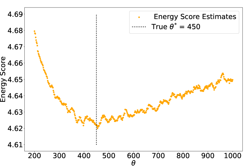
(a) Gaussian Spatial copula

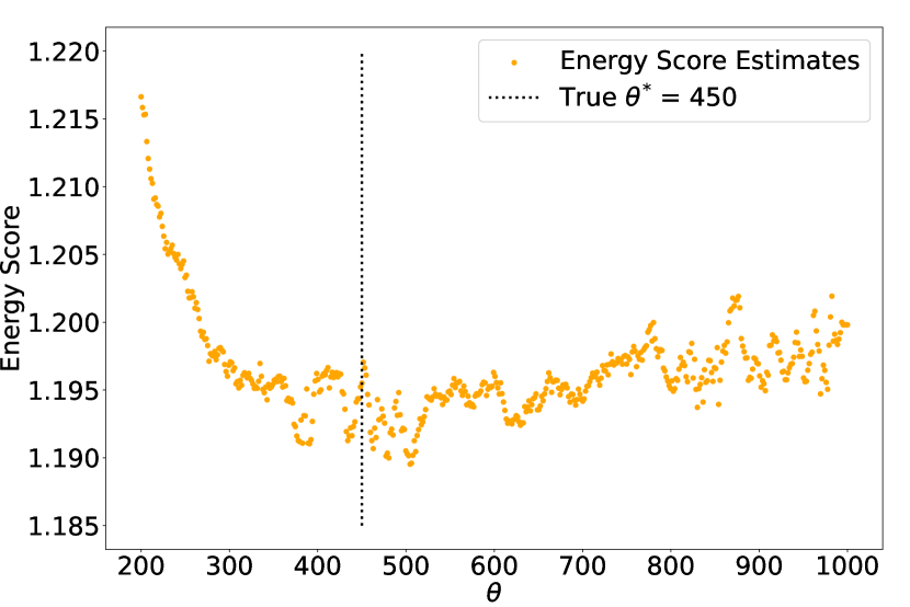
(b) Censored Latent Spatial Gaussian copula

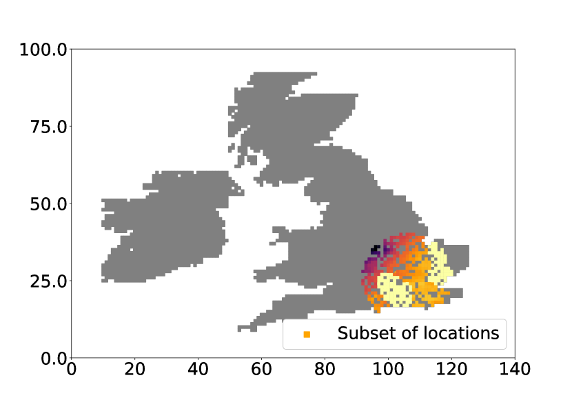
(c) Subset of locations

Figure 1: Simulation study: Lengthscale ($\theta$) plotted against scoring rule estimates for simulated data in two experiments. The inference is done in (a) using a regular Gaussian copula and in (b) with a censored Gaussian copula according to estimated marginal densities of rainfall. The simulated data originates from a subset of locations from the UK, shown in (c).

4.4 Inference on simulated data

To empirically validate our estimation procedure, we perform inference of $\theta$ from simulated data using a spatial Gaussian copula and a censored latent spatial Gaussian copula with known censoring thresholds. For these experiments, we construct $\mathcal{D}$ as described in Appendix B, considering a subset of 400 locations from our UK rainfall data set, as shown in Figure 1(c).

Inference of $\theta$ from simulated data using a Gaussian spatial copula

We simulate data consisting of 5000 independent samples from a Gaussian spatial copula for the 400 locations specified in Figure 1(c), with covariance matrix $\Sigma(\mathcal{D}^{*}|\theta=450)$ constructed using the Matérn kernel. The unbiased estimate of the energy score, obtained from samples with varying $\theta$ value from the same Gaussian spatial copula, is illustrated in Figure 1(a), depicting an estimate in accordance with the true parameter value $\theta=450$. This shows the effectiveness of our approach for inference of parameters of spatial Gaussian copulas, in addition to the existing theoretical consistency results in Alquier et al. (2022).

Inference of $\theta$ from simulated rainfall data using a censored latent spatial Gaussian copula

We conduct a second experiment by simulating observed data as 5000 independent samples from a censored latent spatial Gaussian copula over the same 400 locations from Figure 1(c) with the same covariance matrix $\Sigma(\mathcal{D}^{*}|\theta=450)$ using the Matérn kernel. The simulation involves sampling from a Gaussian spatial copula and then censoring each sample according to the estimated marginals $F_{i,s}(\cdot|\boldsymbol{\mathcal{H}}_{s})$. By considering each draw to come from a different day, we obtain simulated data $\boldsymbol{\mathcal{Y}}_{s}$ over a period of 5000 days from 1999 onwards. We present the unbiased energy score estimate in Figure 1(b) plotted against $\theta$ parameter values, illustrating the curvature of the lengthscale with an arch around the desired value, exemplifying our approach’s validity for estimating $\theta$ in the presence of censored data.

5 Real Data Scenario

Finally we apply our approach to the data set presented in Section 2. We conduct a comprehensive evaluation by comparing our proposed method with other benchmark methods using standard diagnostics of probabilistic forecasts [Appendix D] in Section 5.1. We then assess the spatial coherence of the generated samples from all these methods in Section 5.2. Finally, we investigate the effect of varying lengths of training data on the performance of our approach in Section 5.3.

5.1 Comparison with benchmark models

We begin by comparing our method (denoted Cens-JGNM) to two competing benchmark methods: the variational auto-encoder generative adversarial network (VAE-GAN) (Harris et al., 2022) and the convolutional conditional neural process (ConvCNP) (Vaughan et al., 2021). Both these methods as well as our own were fitted to the grided data detailed in Section 2.1 spanning a 20-year period, divided into a training set from 1979 to 1993 and a validation set from 1993 to 1999. We then compare their forecasting capabilities on a held-out test set of 20 years, from 1999 to 2019.

Remark: It is worth reiterating that our data does not include precipitation weather forecasts as a predictor, unlike the above-mentioned studies of Harris et al. (2022); Vaughan et al. (2021). Consequently, the performance of the benchmark methods obtained in their respective articles cannot be directly compared with the performances presented in this study (of the benchmarks as well as our approach). The inclusion of precipitation CM predictions would improve a model’s forecasting capabilities for rainfall.

We begin by looking at the Area Under the Curve (AUC) [Appendix D.1] resulting from a calibration task, as shown in Figure 2(a), with corresponding Return Operating Curves (ROCs) reported in Appendix E. The AUC achieved by the Cens-JGNM is slightly higher than that of the ConvCNP, and both remain constant across different precipitation amounts. The VAE-GAN’s AUC is generally lower than the two other methods and deteriorates for higher precipitation amounts. As the AUC diagnostic is largely influenced by marginal densities, it exemplifies the benefit of an explicit marginal model as done by the Cens-JGNM and ConvCNP in this context.

In Figure 2(b), we show rank histograms [Appendix D.2] to investigate calibration. The Cens-JGNM and ConvCNP have almost identical performances, displaying a close fit to the ideal rank, which we attribute to their similar form of marginal densities with the adoption of a Gamma mixture model. The slight misalignment of ranks on the far right for the two aforementioned approaches suggests that the parametric form is not entirely accurate in the tail, and could benefit from a more appropriate treatment of extreme values. On the other hand, the VAE-GAN displays a poor performance characteristic of under-dispersion with ranks over-represented at 0 and 1, arguing in favour of a parametric approach for marginal densities.

The Empirical Cumulative Density functions (ECDFs) [Appendix D.3] of each approach are studied in Figure 2(c). The Cens-JGNM has the closest fit to the empirical frequency, suggesting it has the best calibration out of the three models. As this diagnostic is aggregated over space, we attribute ConvCNP’s overestimation of realised rainfall to the lack of explicit dependence modelling leading to miss-calibrated joint forecasts. The under-dispersion and non-explicit modelling of zero values of the VAE-GAN is exemplified with an incorrect intercept at $0\,mm$ and a lower frequency for higher amounts.

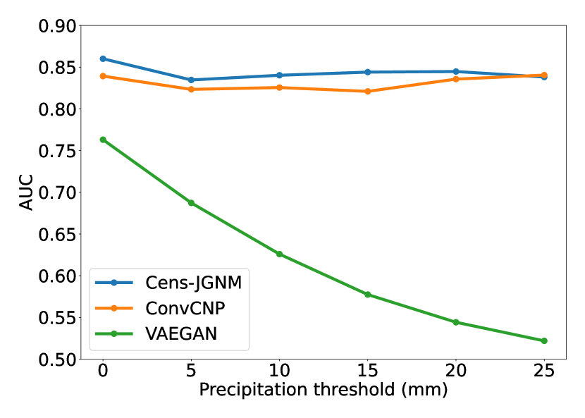
(a) AUC

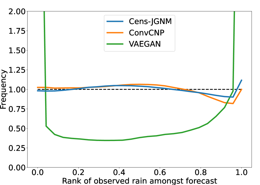
(b) Rank histogram

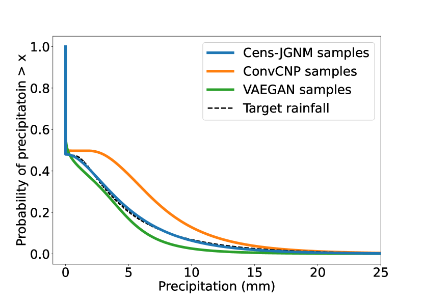
(c) ECDF

Figure 2: Calibration diagnostics: We show in (a) AUCs [Appendix D.1], (b) Rank histograms [Appendix D.2] of the rank of precipitation observations against simulated samples and (c) ECDFs [Appendix D.3] for our Cens-JGNM approach compared to ConvCNP and VAE-GAN benchmarks. Figures 2(a) and 2(b) indicate the appropriate treatment of marginal densities by the Cens-JGNM and ConvCNP both employing explicit Gamma densities as opposed to the implicit approach of the VAE-GAN. Figure 2(c) reveals that the Cens-JGNM obtains the best calibration, the VAE-GAN incorrectly captures 0 values, and the ConvCNP overestimates rainfall.

5.2 Spatial coherence

For the same set-up as in Section 5.1 above, we analyse each approach’s ability to accurately capture spatial dependence in generated samples.

Figure 3 examines the spatial cross-correlation between a centre point and the rest of the locations [Appendix D.4] for observed data and samples from each modelling approach. The Cens-JGNM is the best approach at replicating the cross-correlation of observations, displaying correct dependence for close and medium distances from the central point. The ConvCNP shows minimal dependence across all locations resulting from insufficient modelling of a dependency structure in its approach. The VAE-GAN captures partial dependence at short distances but fails to do so for locations further away. We believe the most significant improvement offered by the Cens-JGNM is its effectiveness at capturing spatial dependence at much larger scales than competing approaches. We attribute this performance to the spatially informed construction of the censored latent spatial Gaussian copula detailed in Section 4.1. Moreover, we believe it is possible to capture even further dependencies by incorporating more information in the initial distance matrix $\mathcal{D}$ such as differences in predictor values or additional spatially relevant variables.

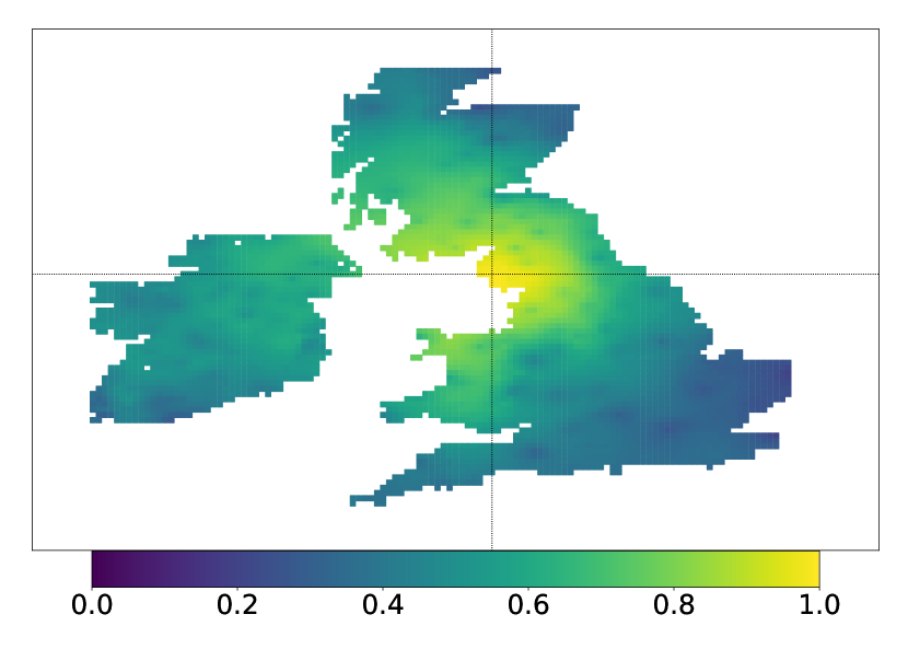
(a) Observed

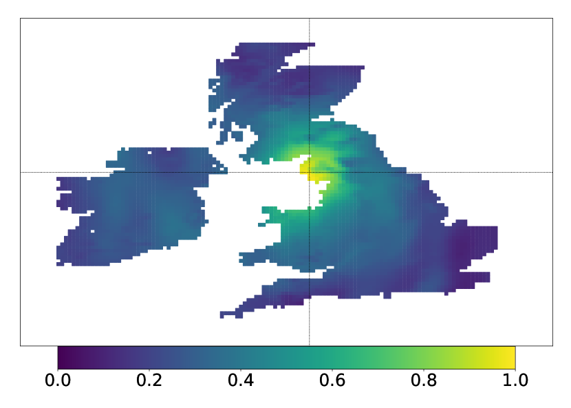
(b) Censored JGNM

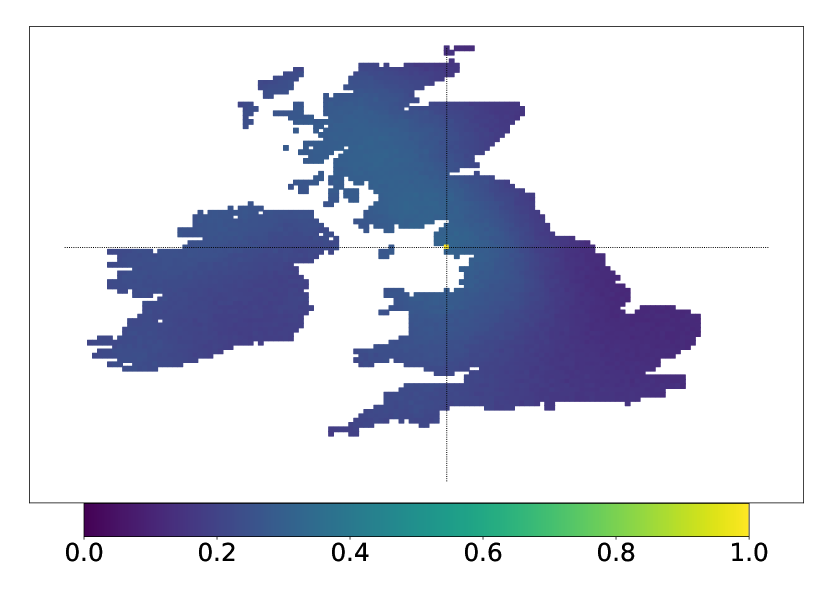
(c) ConvCNP

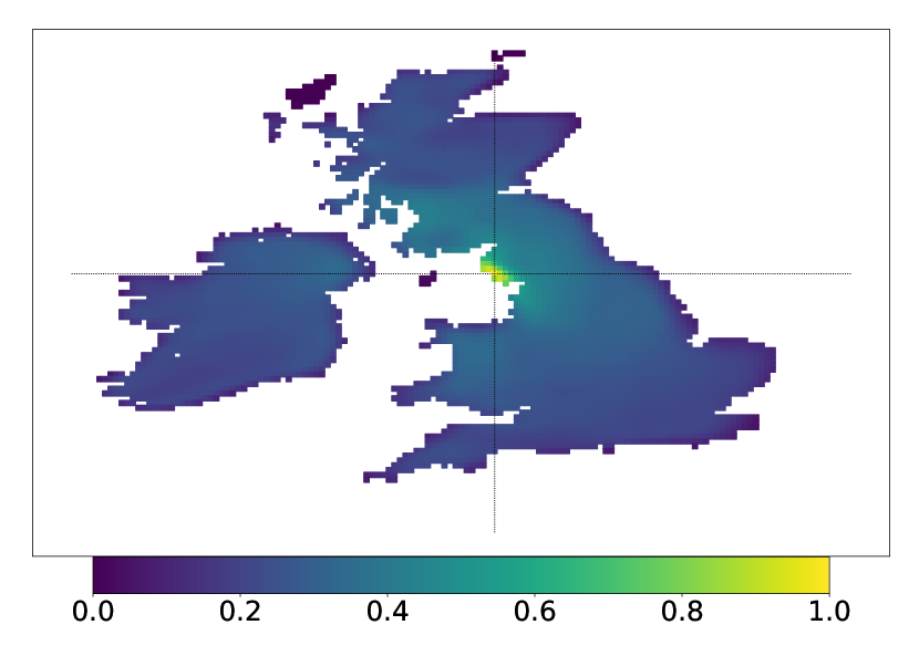
(d) VAE GAN

Figure 3: Spatial coherence: We show cross-correlation plots [Appendix D.4] for (a) observations as well as samples from the (b) Cens-JGNM, (c) ConvCNP and (d) VAE-GAN. As evidenced by the plots, our Cens-JGNM is the most effective approach at capturing spatial dependence while the VAE-GAN and ConvCNP capture minimal and short-scale dependence only, respectively.

We conclude our comparison with Table 1, presenting various diagnostics metrics assessing calibration, accuracy and spatial dependence. these metrics include the Continuous Ranked Probability Score (CRPS) [Appendix D.5], energy score [Appendix C], variogram score [Appendix D.6] as well as the Root Mean Square Error (RMSB) and Mean Absolute Bias (MAB) [Appendix D.7]. Our Cens-JGNM outperforms both benchmarks on all diagnostic metrics, demonstrating its superior spatial as well as point-wise prediction abilities.

Diagnostic Metrics
Model	Cens-JGNM	ConvCNP	VAE-GAN
CRPS	1.1613	1.6536	4.5059
Energy Score	2.6184	3.1003	3.2127
Variogram Score	2,949,584	7,914,394	9,841,903
RMSB	3.8642	4.3073	4.8861
MAB	1.839	3.0266	1.9865

Table 1: Comparison with benchmarks: Numerical diagnostics for the Cens-JGNM (ours) against ConvCNP and VAE-GAN. Our approach beats competitors across all metrics.

5.3 Robustness on Length of Training Data Set

In addition to comparing our approach against benchmarks, we appraise the robustness of the Cens-JGNM to reduced amounts of data. We train a Cens-JGNM on increasingly smaller data samples and compare the resulting forecasts on common test data. There are four Cens-JGNM versions in total, respectively fitted on 4 years of data (01/1985 to 06/1989), 6 years (1983 to 06/1989), 8 years (1981 to 06/1989) and finally 10 years (1979 to 06/1989). All are tested on the same 30 years of data, from 07/1989 to 07/2019. We use the same diagnostics as in Sections 5.1 and 5.2 above, to determine whether the performance of our method suffers in settings with a lack of data.

We begin by inspecting the AUCs (with ROCs reported in Appendix E) in Figure 4(a). The different sample sizes have no significant effect, as all four versions achieve similar AUCs. The models are better calibrated for lower rainfall events, which is explained by the reduced fitting data, implying that fewer extreme observations are used to train each model. We also compare their rank histograms in Figure 4(b), which again show no significant difference or trend across model versions. From Figure 4(c), showing ECDFs, it is again indicated that periods above 4 years of data are sufficient to ensure the strong performance of our model as all four versions display nearly identical performance. Importantly, performance of these versions match the performance of the Cens-JGNM trained on 20 years of data in Section 5.1.

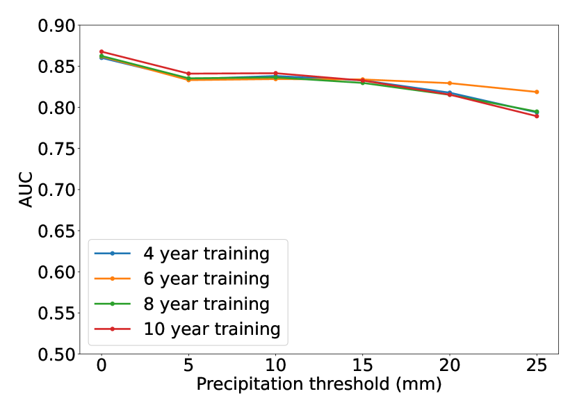
(a) AUC

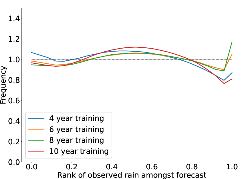
(b) Rank Histogram

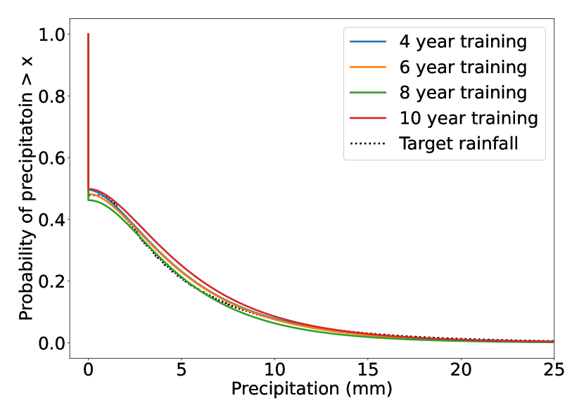
(c) ECDF

Figure 4: Robustness: We show the (a) AUCs, (b) rank histograms, and (c) ECDFs for the Cens-JGNM model versions fitted on decreasing amounts of data (10, 8, 6, and 4 years). The diagnostics show no trend across data size, indicating that the Cens-JGNM is robust to reduced amounts of data.

To assess the spatial dependence of the model versions, cross-correlation plots are shown in Figure 5. All four versions capture the spatial structure effectively, with no clear trend with respect to data amount. The performance of the Cens-JGNM on 20 years of data, shown in Figure 3, is matched even with reduced fitting sample sizes. In Table 2, we compare the metrics of the four model versions.

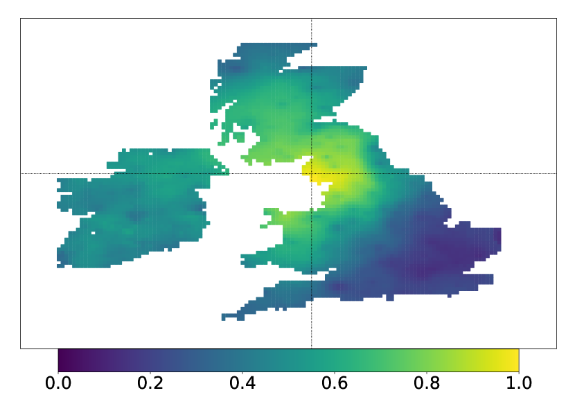
(a) Observed

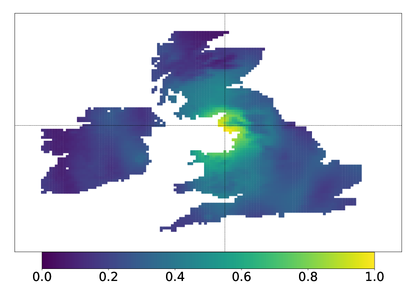
(b) 10 years

(c) 8 years

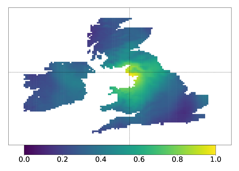
(d) 6 years

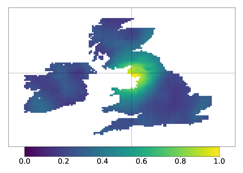
(e) 4 years

Figure 5: Robustness: Cross-correlation maps for different fitting periods of our Cens-JGNM model. All four Cens-JGNM model versions effectively capture the spatial structure, matching the performance of our approach fitted on 20 years of data in Figure 3(b), demonstrating our approach’s robustness to a smaller training sample size.

Diagnostic Metrics for probabilistic forecasting
Metric	4 years	6 years	8 years	10 years
CRPS	1.2640	1.2301	1.178	1.3449
Energy Score	2.6026	2.5669	2.5693	2.6757
Variogram Score	3,856,752	7005992	7027719	7793053
RMSB	4.0971	4.0882	4.1642	3.9889
MAB	1.928	1.9795	1.735	2.107

Table 2: Robustness: Numerical diagnostics for the Cens-JGNM approach fitted on multiple reduced amounts of training data. The results indicate no trend in the performance of our approach across training data quantity.

6 Related Work

In this section, we review some existing literature connected to our work. We being in Section 6.1 by discussing other methods of forecasting rainfall in a univariate context. Next, in Section 6.2, we explore the estimation issues present in copulas when the likelihood becomes complicated to evaluate or directly unavailable. Finally, we describe alternative approaches to probabilistic rainfall forecasting than our two-step procedure in Section 6.3.

6.1 Marginal rainfall estimation

In Little et al. (2008), a study on GLMs used for rainfall density estimation with Markovian assumptions on temporal dependence recommends the use of a Bernoulli-Gamma mixture or an ensemble model, motivating our JGNM parametric choice. This comparison study further reinforces the findings of (Das, 1955; Fealy and Sweeney, 2007; Ailliot et al., 2015; Holsclaw et al., 2017; Bertolacci et al., 2019; Xie et al., 2023), all reporting success with marginal models based on Gamma densities. PCA regression was used in Li and Smith (2009) for precipitation downscaling using CM variables together with mean sea level pressure (MSLP) measurements, alleviating the underprediction problems faced by CMs. Our JGNM can be seen as a generalisation, where the refinement of variables used in a regression model is made in a data-driven way. Quantile regression is used by Tareghian and Rasmussen (2013) to get daily precipitation distributions by conditioning on CM outputs, increasing the flexibility in the selection of predictors, which our JGNM increases even further. Su et al. (2019) applied Bayesian model averaging (BMA) and stepwise regression models (SRMs) to downscaling. Our approach incorporates a pre-treatment of predictors as in SRMs with uncertainty quantification as in BMA, combining both strengths under a single approach.

Deep Learning (DL) methods have been used effectively in Geosciences, such as Li et al. (2021) applying DL methods to forecast location-wise densities of solar energy. In Adewoyin et al. (2021), expanding on previous DL models applied to rainfall forecasting such as Shi et al. (2015); Vandal et al. (2017); Miao et al. (2019) and Pan et al. (2019), the authors achieved state-of-the-art performance in point-wise prediction, showing that DL methods can be used to downscale rainfall based on CM forecasts. We directly improve on their approach by incorporating uncertainty quantification in the marginals.

6.2 Copula estimation problems

As is common when the copula is latent or in the presence of zero-inflated data (both being the case in our work), MLE-based inference becomes complicated or unavailable and alternatives need to be considered.

For extreme rainfall modelling, Huser and Wadsworth (2019) assume a censored copula for extreme values, targeting the full likelihood for inference, but only for up to 15 locations, noting that a high dimension is a limiting factor for Gaussian copulas, reinforcing the conclusions of Huser et al. (2017). Modelling extreme rainfall through a Brown–Resnick process, Richards and Wadsworth (2021) resort to a composite likelihood approach as an alternative to a computationally unfeasible MLE. More recently, in Richards et al. (2022) and Richards et al. (2023), authors use a censored Gaussian copula model for the dependence of extreme rainfall events, circumventing the unavailable likelihood by adopting a pseudo-likelihood approach with spatially-informed sub-sampling. Outside of rainfall forecasting, Dobra and Lenkoski (2011) model graphical binary and ordinal variables in a Bayesian framework with a latent Gaussian copula, requiring an approximation to the likelihood function with the extended rank likelihood of D. Hoff (2007). Thus, as was summarised in Huser et al. (2016), while the use of these pseudo-likelihoods allows for inference, performing inference in higher dimensions remains an open problem. Our minimum scoring estimate approach provides a direct solution by not relying on likelihoods, additionally ensuring exact and computationally efficient parameter inference.

In the presence of zero-inflated data, Yoon et al. (2020) introduce a truncated latent Gaussian copula as an analogue to censored copulas and develop an estimator for the latent covariance matrix expanding on a rank-based procedure from Fan et al. (2017). This approach is expanded by Chung et al. (2022) to a Bayesian setting on graphical models for zero-inflated count-data data where inference is performed using Gibbs sampling. While their approach allows for higher dimensions, it is framed inside the Bayesian paradigm, whereas our minimum scoring rule approach is exact and can be used in both frequentist and Bayesian settings (with extensions following the works of Pacchiardi and Dutta (2021)).

Recent advances in likelihood-free inference have led to the development of alternative methods for copulas inference. Alquier et al. (2022) use the maximum mean discrepancy (MMD) as a function to minimise in order to learn the parameters of copulas, obtaining a covariance estimator robust to miss-specification. Similarly, Janke et al. (2021) employ the energy distance (a possible instance of the MMD) as a loss function in the training of a generative network to approximate a copula distribution, avoiding the necessity for hyperparameters for the MMD. Our work extends their approaches to a spatial setting while accounting for censored observations.

6.3 Alternative probabilistic forecasting approaches for rainfall

Non-homogeneous hidden Markov models for rainfall occurrence are considered by James P. Hughes and Charles (1999) with extensions for amounts by Charles et al. (1999), modelling occurrence and amount of rainfall separately, which we do jointly with our JGNM. We further avoid their conditional independence assumptions on the spatial dependence structure with our censored copula approach. Frost et al. (2011), a review of six downscaling methods (namely Chandler (2002); Timbal (2004); McGregor (2005); Mehrotra and Sharma (2007); Chiew et al. (2009) and a HMMs-based (Charles et al., 1999) implementation of Kirshner (2007)), found that HMMs displayed weaknesses in capturing spatial correlation. Applying Bayesian HMMs to rainfall, Song et al. (2014) (expanding on the approach of Li and Smith (2009)) uses a covariance matrix construction with spatial distances used only in error correlation. Holsclaw et al. (2017) assume a more complicated time-dependency in transition probabilities, which calls for a Polya-Gamma-based MCMC sampling scheme. Bertolacci et al. (2019) use a spatial structure captured through a Gaussian process with marginal densities modelled by mixtures of expert models. Our approach extends these methods with direct and richer spatial modelling through the censored latent Gaussian copula.

Ensemble Model Output Statistics (EMOS), introduced by Gneiting et al. (2005) and improved by the works of Dabernig et al. (2017); Möller and Groß (2016, 2020), models rainfall using an appropriate density of which parameters are estimated with linear regression equations incorporating spatio-temporal effects. Rasp and Lerch (2018) use neural networks instead of linear regression equations, further improved by Mlakar et al. (2023), performing estimation jointly across all future times and locations. Our approach similarly estimates distributions jointly in a spatio-temporal manner, however, we additionally employ the censored latent copula to impose the correct spatial dependence for any given forecast.

Machine learning approaches include Watson et al. (2020), with the use of Generative Adversarial Networks (GANs) to increase the resolution of rainfall forecasts while simultaneously aiming to correct biases. This work was expanded upon by Price and Rasp (2022) by using a conditional GAN based on coarse weather variables. Similarly, Harris et al. (2022) substitutes the GAN generator with a variational auto-encoder for conditional forecasts, adapted to cyclone-induced rainfall by Vosper et al. (2023). Alternatively, Pacchiardi et al. (2022); Chen et al. (2022) use generative neural networks with the energy score as a loss function to avoid the problematic training of GANs. All these approaches learn an implicit likelihood and suffer from the drawbacks such as the inability of generating zero values. Our JGNM model ensures explainability and a proper fitting of zero values and we compared our spatial dependence to the study of Harris et al. (2022), demonstrating improved performance. Further, our model can be evaluated on new locations after training, unlike most of these methods. Vaughan et al. (2021) employ a convolutional conditional neural process model with parametric marginals, explicit modelling of zero values and inclusion of out-of-sample locations. Their approach is very similar to the JGNM, although their model fails at capturing spatial dependence to the same extent as our censored copula method, as evidenced in Section 5.1. Ascenso et al. (2023) use a convolutional network approach with a modified loss function to enforce the spatial coherence of rainfall. We have a similar focus on spatial dependence with the energy score but additionally provide uncertainty quantification and interpretability.

7 Conclusion

In this paper, we introduced a novel method for spatio-temporal joint forecasts of zero-inflated data. We described our first component joint generalised neural model as a distributional learner capturing temporal trends in conjunction with surrounding information to describe distributions for quantities of interest. The JGNM is very flexible and can be evaluated at any location, even one outside of the learning set. We also introduced censored latent Gaussian copulas as an answer to the spatial dependence modelling of censored data. We motivated the unavailable likelihood prohibiting the use of regular MLE-based methods, and offered a scoring-rule-based alternative, resulting in cheaper and more robust parameter inference. Our censored latent Gaussian copula methodology allows for the automatic inclusion of new locations, making our complete approach capable of accommodating additional locations added to the model without requiring parameter re-estimation. We compared our model to competitive benchmarks focusing on the same task (Vaughan et al., 2021; Harris et al., 2022). We demonstrated our model’s ability to correctly capture uncertainty to the same or better extent as competitors. Furthermore, we showcased our model’s superior capture of spatial dependence over benchmarks, rendering our approach better suited for scenarios where spatial coherence is desired.

This work is an important improvement towards more reliable post-processing techniques as well as precipitation forecasts capable of correctly capturing uncertainty and spatial dependence. Moreover, while the main motivation of our work is rainfall forecasting, our methodology can effortlessly be applied to any spatio-temporal probabilistic forecast, with or without censoring. Therefore, we believe that our work is not only of interest to the weather science community but indeed relevant to the broader multivariate forecasting community.

A possible extension of our model is the construction of the covariance matrix of the latent censored Gaussian copula in Section 4.1. Specifically, in the initial distance $\mathcal{D}$, one could include information on differences in weather variables to better capture the spatial dependence. In fact, it is possible to extend our copula approach to explicitly capture temporal dependence by adapting the kernel parameter according to temporal information. Other improvements particular to the modelling of extreme rainfall events could be made to the JGNM by considering extreme value distributions (Behrens et al., 2004; MacDonald et al., 2011; Ding et al., 2019; Gao et al., 2021; Richards et al., 2022), either entirely or by adding them as a mixture term in the tail. Finally, we acknowledge that imposing a Gaussian covariance structure, while computationally appealing and leading to easy spatial modelling, might be too restrictive, especially for extreme variations in rainfall levels at close-by locations. In this context, we could consider other types of copulas, no longer restricted to Gaussian dependence structures (Janke et al., 2021; Wadsworth and Tawn, 2022; Richards et al., 2023).

Acknoledgement

D.H. is funded by the Center for Doctoral Training in Mathematical Sciences at Warwick. R.A is funded by the University of Warwick and Southern University of Science and Technology. R.D. is funded by EPSRC (grant nos. EP/V025899/1 and EP/T017112/1) and NERC (grant no. NE/T00973X/1).

Appendix A Neural Network Architecture

Implementation-wise, the JGNM operates on 6-hourly low resolution model fields $\boldsymbol{\mathcal{X}}_{j}\in\mathbb{R}^{4{\times}20{\times}21{\times}6}$ from the ERA5 data set [Hersbach et al., 2020] to output the set of 3 target variables $\mu_{s},\phi_{s},\rho_{s}\in\mathbb{R}^{100{\times}140}$, which parameterise predictive distributions for daily total rainfall for a 28-day period. Here the subscript $j$ indicates the 6-hourly units of time as opposed to the daily subscript $s$.

Similar to the approach in Adewoyin et al. [2021], we initially use bi-linear interpolation to map the weather variables from a ${20{\times}21}$ grid to a ${100{\times}140}$ grid. Then, for separate ${16{\times}16}$ spatial subsections of the interpolated grid, we pass the 6-hourly data of all 6 weather variables. This results in our input being of dimension (28$\cdot$4${\times}$16${\times}$16${\times}$6) represented by the matrices $\boldsymbol{x}_{j}$ with $j\in\{1,\ldots,112\}$ in Figure 6.

Next, a time distributed 2D convolution layer (TD2L) is used to transform each $\boldsymbol{x}_{j}$ to a hidden representation where, importantly, the layer applies the same instance of a 2D convolutional unit to each time-wise unit of a temporal sequence. In our setting the channel dimension of the hidden representation $d$ is 64 such that $TD2L(\mathcal{X}_{j})\rightarrow{h}^{TD2L}_{j}\in\mathbb{R}*{28\cdot 4{\times}16{\times}16{\times}64)}$.

The stacked convolutional LSTM (CLSTM) [Shi et al., 2015] layers contain a stack of 2 bi-directional CLSTM layers. Skip connections are employed between successive layers. The outputs from the backward and forward CLSTM units are combined through concatenation. In our experiments, the Conv-LSTM layers have input dropouts of 0.25 and recurrent dropouts of 0.35.

The time distributed temporal downscaling layer (TDTD) performs temporal downscaling on the output of the stacked Conv-LSTM. Specifically, the CLSTM output ${h}_{j}$, $j\in\{1,\ldots,112\}$, is transformed from a sequence of 112 tensors to 28 tensors representing a shift from a 6 hourly information set to a daily information set $\boldsymbol{h}_{s}$, $s\in\{1,\ldots,28\}$. In this case, the time-distributed operation is implemented by performing the same downscaling operation on non-overlapping groups of 4 sequential ${h}_{j}$. The TDTD is comprised of a convolutional self-attention layer, responsible for the temporal downscaling, a nonlinear Gaussian error linear unit (GeLU) [Hendrycks and Gimpel, 2016] activation and two convolutional 2D layers. In Appendix A.1 we discuss the convolutional self-attention layer in further detail.

In the convolutional self-attention layer, we use multiple heads in order to capture the notion that the hidden representation chosen to represent the one time period at a coarser time resolution, should be a dynamically weighted aggregation of hidden representations corresponding to the same time step but at a finer resolution. The use of multiple heads attention allows the model to extract a different type of feature for each head, capturing various aspects of the output sequence from the stacked Conv-LSTM. In Appendix A.1, we provide a thorough explanation of how this module works.

Finally, our Time Distributed Mean Function Layer has three Single Layer Perceptrons, with each one acting as a mean function, also known as inverse link function, for each parameter in the three-parameter distribution we study. Each perceptron operates on each input from the layer below to produce an estimate for each timestep, as shown in Figure 6. In sub-section A.2 we provide detail on the GLM mean functions used.

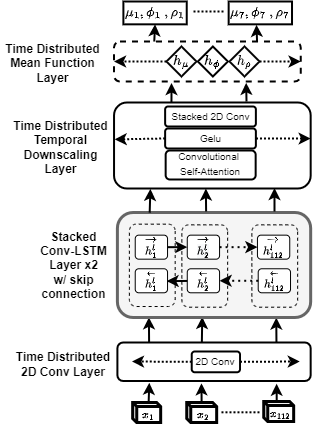
Figure 6: JGNM architecture. This figure depicts our joint generalised neural model, which outputs parameters for a 3-parameter distribution. We use it to parameterize predictive Zero-Gamma mixture distributions for the rainfall over 28 consecutive days. The Sequence Length of 3D tensors between layers is contracted in the Time Distributed Temporal Downscaling Layer (TDTD), as our input has a 6-hour frequency, while the output is daily.

A.1 Convolutional self-attention (CSA)

At its core, this module reduces a sequence of three-dimensional images from a sequence length of $t_{i}$ to a sequence length of $t_{o}$ accomplishing a decrease of factor $s$.

Given an input tensor $x\in\mathbb{R}^{(b,t_{i},h,w,c)}$, where $b$ is the batch size, the CSA performs the following operations.

First a positional embedding $\text{pos\_embd}\in\mathbb{R}^{1,s,d}$ as a trainable weight matrix, is retrieved where $d=h{\times}w{\times}c$.

If we consider the input tensor $x$ to be comprised of non-overlapping sub-sequences $x_{[j,j+s]}$, then for every sub-sequence we reshape its dimensions as $(b,t_{i},h,w,c)\rightarrow(b,t_{i},d)$ followed by adding pos_embed to each sub-sequence, forming a new set of sub-sequences $x^{\prime}$ with information on their relative position as

$$x_{[j,j+s]}^{\prime}=x_{[j,j+s]}.\text{reshape}(b,t_{i},d)+\text{pos\_emb}.$$

Attention modules employ three types of tensors, query, key, and value in order to perform a weighted average. For each sub-sequence $x_{[j,j+s]}^{\prime}$ we create a query input by averaging the sub-sequence tensor $x_{[j,j+s]}^{\prime}$ along the sequence length dimension. Therefore, the query, key, and value inputs $(x^{q},\,x^{k}\text{ and }x^{v})$ are are given by

$$x^{q}_{[j,j+s]} =x_{[j,j+s]}^{\prime}.\text{mean}(\text{{dim}}=-2)$$

$$x^{k}_{[j,j+s]} =x_{[j,j+s]}$$

$$x^{v}_{[j,j+s]} =x_{[j,j+s]}.$$

Then the query input, key input and value input are linearly transformed into query $Q$, key $K$, and value $V$ vectors using learned weight matrices $W^{Q}$, $W^{K}$, $W^{V}$ and $W^{O}$ respectively. This process is performed for each attention head $h\in H$. For a given head $h$, we have:

$$Q_{[j,j+s]}^{h} =x_{[j,j+s]}^{q}\cdot W^{Q}_{h}$$

$$K_{[j,j+s]}^{h} =x_{[j,j+s]}^{k}\cdot W^{K}_{h}$$

$$V_{[j,j+s]}^{h} =x_{[j,j+s]}^{v}\cdot W^{V}_{h}$$

$$\text{where }W^{Q},W^{K},W^{V}\in\mathbb{R}^{d,d^{hidden}\text{.}}$$

Next, scaled dot-product attention computes the dot product of the query $Q_{h}$ with all keys $K_{h}$, divides each by the square root of the dimension of the key vectors $\sqrt{d^{k}}$, and applies a softmax function to obtain the weights on the value vectors $V_{h}$:

$$\text{head}_{h}=\text{softmax}\left(\frac{Q_{[j,j+s]}^{h}(K_{[j,j+s]}^{h})^{T}}{\sqrt{d^{k}}}\right)V_{[j,j+s]}^{h}.$$

Afterward, the output of each head is concatenated and then linearly transformed to result in the output sub-sequence:

$$x_{[j,j+s]}^{(output)} =\text{Concat}(\text{head}_{1},...,\text{head}_{H})\cdot W^{O}\text{where }W^{O}\in\mathbb{R}^{d^{(hidden),d^{(output)}})}.$$

Finally, the output is reshaped to a subsequences of $x^{(output)}_{[j,j+s]}\in\mathbb{R}^{(b,t_{i},c,h,w)}$, demonstrating effective temporal downscaling on a sequence of 3-dimensional arrays. In our implementation we use the following values: $h{=}4,\,w{=}4,\,c{=}6,\,s{=}4,\,d^{(hidden)}{=}64,\,d^{(output)}{=}64,\,H{=}4$.

A.2 Time Distributed Mean Function Layer

In Table 3 we list the mean function, also known as the inverse link function, used per parameter for the Zero-Gamma mixture density. Since in a neural network setting, the mean function can be interpreted as the activation function, we aim to select an activation function with a range appropriate for the target parameter that also provides stability during training.

	parameter range	mean function
$\mu$	$[0,\infty)$	$(6.0\cdot\text{ReLU}(x+0.4))+1\exp^{-6}$
$\phi$	$[0,\infty)$	$(6.0\cdot\text{ReLU}(x+0.5))+1\exp^{-6}$
p	$[0,1]$	$\text{sigmoid}{(x)}$

Table 3: GLM mean functions: Mean function used in the Time Distributed Mean Function Layer of the Zero-Inflated JGNM

Appendix B Construction of Distances Matrix

Within a latent Gaussian copula, one needs to estimate a covariance matrix $\Sigma$, which we construct as a function of an initial distance matrix $\mathcal{D}$. As we want the copula to be spatially informed, we consider the latitude and longitude of locations as well as the topography given by geopotential height. Taking $D$ to be the matrix of pair-wise Euclidean norms of (latitude, longitude) and $T$ that of pair-wise Euclidean norms of topography between locations, we construct the distance matrix $\mathcal{D}$ by computing

$$\mathcal{D}=a\cdot D+(1-a)\cdot\frac{T}{70}.$$

Here, we divide $T$ by 70 in order to normalise values between the two contributing matrices. The coefficient $a$ serves to adjust the relative importance of each matrix, where $a\to 1$ makes the dependence within our approaches samples rely on geographical distances only while $a\to 0$ makes the samples rely uniquely on topography. We treat it as a hyperparameter, setting it to $0.9$ as this produced the most realistic samples using in our study.

Appendix C Scoring Rules as a Divergence

Assume we have observed data from distribution $\mathcal{P}^{*}$ and want to choose a parameter $\boldsymbol{\theta}$ which parameterises a second distribution $\mathcal{P}^{\boldsymbol{\theta}}$ such that the two distributions are as close to each other as possible. A divergence $D$ is then defined as a function of two distributions such that (i) $D(\mathcal{P}^{*}||\mathcal{P}^{\boldsymbol{\theta}})\geq 0$ and (ii) $D(\mathcal{P}^{*}||\mathcal{P}^{\boldsymbol{\theta}})=0\iff\mathcal{P}^{*}=\mathcal{P}^{\boldsymbol{\theta}}$. Therefore, a divergence can be used to optimise a parameter to recover the best possible model $\mathcal{P}^{\boldsymbol{\theta}}$ for the data generating distribution $\mathcal{P}^{*}$ .

One possible choice of divergences are scoring rules (SRs). As defined in Gneiting and Raftery [2007], a scoring rule $S(\mathcal{P},\mathbf{x})$ is a function between a distribution $\mathcal{P}^{\boldsymbol{\theta}}$ and observed data $\mathbf{x}$ as a realisation of a random variable $\mathbf{X}\sim\mathcal{P}^{*}$. Then the expected scoring rule is defined as $S(\mathcal{P},\mathbf{x}):=\mathbb{E}_{\mathbf{Y}\sim\mathcal{P}^{*}}S(\mathcal{P}^{\boldsymbol{\theta}},\mathbf{Y})$. The SR is termed proper if relative to a set of distributions $\mathbf{P}$, if the expected SR is minimised when $\mathcal{P}^{*}=\mathcal{P}^{\boldsymbol{\theta}}$:

$$S\left(\mathcal{P}^{*},\mathcal{P}^{*}\right)\leq S\left(\mathcal{P}^{\boldsymbol{\theta}},\mathcal{P}^{*}\right)\,\,\forall\,\mathcal{P}^{\boldsymbol{\theta}},\mathcal{P}^{*}\in\mathbf{P}.$$

Furthermore, a SR is termed strictly proper, if the minimisation above is unique:

$$S\left(\mathcal{P}^{*},\mathcal{P}^{*}\right)<S\left(\mathcal{P}^{\boldsymbol{\theta}},\mathcal{P}^{*}\right)\,\,\forall\,\mathcal{P}^{\boldsymbol{\theta}},\mathcal{P}^{*}\in\mathbf{P}\text{ s.t. }\mathcal{P}^{*}\neq\mathcal{P}^{\boldsymbol{\theta}}.$$

By considering the quantity $D_{SR}(\mathcal{P}^{*}||\mathcal{P}^{\boldsymbol{\theta}}):=S\left(\mathcal{P}^{*},\mathcal{P}^{\boldsymbol{\theta}}\right)-S\left(\mathcal{P}^{*},\mathcal{P}^{*}\right)$ for a strictly proper SR, one can see that it defines a divergence. Indeed, (i) is verified by the SR being proper and (ii) is verified by the additional requirement of being strictly proper. This permits the use of strictly proper SRs as divergences to perform inference on parameters of a distribution. For the choice of SR, we introduce the Energy Score as:

$$S_{\mathrm{E}}\left(\mathcal{P}^{\boldsymbol{\theta}},\mathbf{x}\right)=2\cdot\mathbb{E}_{\mathbf{X}^{\prime}\sim\mathcal{P}^{\boldsymbol{\theta}}}\|\mathbf{X}^{\prime}-\mathbf{x}\|_{2}^{\beta}-\mathbb{E}_{\mathbf{X}_{1}^{\prime},\mathbf{X}_{2}^{\prime}\sim\mathcal{P}^{\boldsymbol{\theta}}}\left\|\mathbf{X}^{\prime}_{1}-\mathbf{X}^{\prime}_{2}\right\|_{2}^{\beta}$$

where $\beta\in(0,2)$ is a hyperparameter regulating the severity of the divergence for incorrect distributions $\mathcal{P}^{\boldsymbol{\theta}}$. The energy SR is a strictly proper SR for the class of $\mathbf{P}$ such that $\mathbb{E}_{{\mathbf{X}^{\prime}}\sim P}\|{\mathbf{X}^{\prime}}\|^{\beta}<\infty$, see Gneiting and Raftery [2007] and is also known as a rescaling of the energy distance mentioned in section 4.2 . It is possible to obtain unbiased estimates of $S_{\mathrm{E}}\left(\mathcal{P}^{\boldsymbol{\theta}},\mathbf{x}\right)$ by repeated sampling $\mathbf{x}^{\prime}$ from $\mathcal{P}^{\boldsymbol{\theta}}$, as:

$$\hat{S}_{\mathrm{E}}\left(\{\mathbf{x}_{j}^{\prime}:1\leq j\leq m\},\mathbf{x}\right)=\frac{2}{m}\sum_{j=1}^{m}\left\|\mathbf{x}_{j}^{\prime}-\mathbf{x}\right\|_{2}^{\beta}-\frac{1}{m(m-1)}\sum_{\begin{subarray}{c}j,k=1\\ k\neq j\end{subarray}}^{m}\left\|\mathbf{x}_{j}^{\prime}-\mathbf{x}_{k}^{\prime}\right\|_{2}^{\beta}$$

where $\mathbf{x}$ are observations and $\mathbf{x}^{\prime}$ are samples. As such, we have a method for inferring parameters of a distribution by comparing the observations to simulated samples and minimising $D_{SR}$ using the unbiased estimate of the SR. This is equivalent to choosing $\boldsymbol{\theta^{*}}=\operatorname*{arg\,min}\limits_{\boldsymbol{\theta}}\hat{S}_{\mathrm{E}}\left(\mathcal{P}^{\boldsymbol{\theta}},\mathbf{x}\right)$ since the first part of $D_{SR}$ is constant in $\boldsymbol{\theta}$.

Appendix D Description of Diagnostics

D.1 AUC of calibration task

We seek to verify the accuracy of our model’s daily estimated probabilities for a given amount of rainfall compared to the observed amount. To achieve this, we assess the sensitivity of the detection of heavy precipitation. We convert our forecasting task into a classification task by asking the following question: “Will there be precipitation exceeding a given amount?” The answer to this question will depend on a probability threshold, which our model has to surpass in order to emit a signal, or rather, give a positive answer to the question. This threshold $\tau$ is subjective and can be chosen as any value in [0, 1].
For a given threshold, a test that correctly predicts heavy rain (as in rain exceeding a given amount) is known as a true positive. But if the test predicts heavy rain on a day it did not occur, this is known as a false positive. By treating precipitation at each day and point in space as separate independent events, a true positive rate (the proportion of points and days with heavy rain which was correctly detected) and the false positive rate (the proportion of points and days with no heavy rain with a positive signal) can be obtained.
In order to detect heavy rain, we compare the threshold $\tau$ with $1-F_{i,t}(q)$, that is 1 minus the CDF for location $i$ at time $t$ evaluated at the heavy rain value $q\in\mathbb{R}_{\geq 0}$. The higher the value of $\tau$, the more mass under the PDF on the right of $q$ we need in order to be confident enough to issue a positive signal. On the contrary, assuming $\tau=0$, we then classify all forecasts irrespective of location, time, or predictors as a positive.
By changing this threshold $\tau$, we can construct a receiver operating characteristic (ROC) curve plotting the true and false positive rates at each of these thresholds. Different levels of precipitation $q$ can be tested, for example, 5 mm for light rain up to 25 mm for extreme events. The area under the ROC curve (AUC) can be used to assess how well the prediction for different levels of precipitation in the face of uncertainty was captured by the model. The closer the AUC gets to 1, the more confidence we can have in the heavy rainfall prediction capabilities of the examined model.

D.2 Rank histogram

Another way of assessing the calibration of a density is through rank histograms. By sampling $m$ times from our model, we can obtain an empirical distribution $\hat{F}_{i,t}$ for day $t$ and location $i$. Then, we can estimate $F^{-1}_{i,t}(y_{i,t})$ as $\hat{F}_{i,t}(y_{i,t})=\sum_{k=1}^{m}\mathds{1}\{y_{i,t}>y_{i,t}^{(k)}\}$, that is the quantile of the observed rainfall with respect to our model’s simulations $\{y_{i,t}^{(k)}:k\in\{1,\ldots,m\}\}$. We refer to one such quantile as the rank of $y_{i,t}$. By obtaining the rank of observations across days, we can construct a histogram of ranks. If the model is perfectly calibrated, the ranks will be uniformly distributed on $[0,1]$, as should be the case for a CDF of its own realisations. We can assess properties of our model by inspecting the dissimilarities of the histogram to a flat line [Hamill, 2001]. For instance, if the model is over-dispersed, the ranks will tend to group in the middle while under-dispersion will manifest itself as most ranks falling within the extremes of the histogram. Equally, one can determine bias of the model by observing unequal proportions of ranks on either side of the histogram, where an agglomeration on the right is indicative of under-prediction while agglomeration on the left indicates over-prediction.

D.3 Empirical CDF

To further assess the calibration of our model, we test whether the estimated frequency of a type of event (eg. precipitation $>x$) over the testing period has matched the observed frequency. The estimated frequency of achieving a rainfall realisation above a level $x\in\mathbb{R}_{\geq 0}$ is obtained by generating samples from our model and looking at the proportion of samples exceeding $x$. This is then compared to the actual observation frequencies for values higher than $x$. A well-calibrated model’s sample frequency should follow the observation line closely, while a poorly calibrated model will deviate significantly from it. We refer to these plots as empirical cumulative distribution function plots as they correspond to an approximation of $1-F_{i,s}(y_{i,s}|\mathcal{H}_{s})$.

D.4 Cross-correlation plots

To explicitly show the spatial coherence of forecasts we produce cross-correlation plots. These consider the pair-wise correlation between all locations and the center of mass of the UK. We compare the observed cross-correlation against the sampled cross-correlation across all days. The ideal forecast would have a perfectly matching sample cross-correlation plot with the observed one.

D.5 CRPS

We also rely on numerical metrics to evaluate the effectiveness of our approach. Firstly, we consider the continuous ranked probability score (CRPS) [Matheson and Winkler, 1976], written as

$$\operatorname{CRPS}(F_{i,t},y_{i,t})=-\int_{-\infty}^{\infty}(F(y_{i,t}^{{}^{\prime}})-\mathbf{1}\{y_{i,t}^{{}^{\prime}}\geq y_{i,t}\})^{2}\mathrm{\leavevmode\nobreak\ d}y_{i,t}^{{}^{\prime}}$$

which can be shown to be equal to

$$\operatorname{CRPS}(F_{i,t},y_{i,t})=\frac{1}{2}E_{Y_{1},Y_{2}\sim F_{i,t}}\left|Y_{1}-Y_{2}\right|-E_{Y\sim F_{i,t}}|Y-y_{i,t}|.$$

The above expectations can be estimated without bias through repeated sampling from the model. The CRPS is a generalisation of the mean absolute error and indeed simplifies to it when considering a model with point-wise predictions. This metric is applied location-wise and favors well-calibrated forecasts.

D.6 Variogram score

To specifically target the spatial coherence of our model, we resort to the Variogram score, written as:

$$S_{\mathrm{v}}^{(p)}\left(\mathbf{F}_{t},\mathbf{y}_{t}\right):=\sum_{k,l=1}^{m}w_{kl}\left(\left|y_{k,t}-y_{l,t}\right|^{p}-\mathbb{E}_{\mathbf{Y}\sim\mathbf{F}_{t}}\left|Y_{k,t}-Y_{l,t}\right|^{p}\right)^{2}.$$

Again, we can appeal to repeated sampling in order to estimate the expectation. We take $p=1$ for simplicity. The weights $w_{kl}$ are chosen to represent the spatial nature of the problem. As such, we choose $w_{k,l}$ to be 1 over the distance from location $k$ to $l$ and setting $w_{kk}=0$. This score takes into account the whole joint distribution and compares the smoothness of observed data against that of model forecasts. An ideal forecast would have a Variogram score of zero.

D.7 RMSB and MAB

Finally, we assess the models performances by two quantitative metrics: the root mean squared bias (RMSB) and mean absolute bias (MAB). In order to compute these quantities, we need to convert our probabilistic forecasts into point-forecasts. We do this by relying on the median of $m$ forecasts for any given place and time. We can then compute the two metrics as:

$$\mathrm{RMSB}=\sqrt{\frac{1}{n\times T}\sum_{i=1}^{n}\sum_{t=1}^{T}\left(y_{i,t}-\widehat{y}_{i,t}\right)^{2}},\quad\mathrm{MAB}=\frac{1}{n\times T}\sum_{i=1}^{n}\sum_{t=1}^{T}\left|y_{i,t}-\widehat{y}_{i,t}\right|$$

where $\widehat{y}_{i,t}$ is the median for time $t$ and location $i$, $y_{i,t}$ is the equivalent realisation of rainfall and $T$ is the total number of days considered.

Appendix E ROC for Experiments

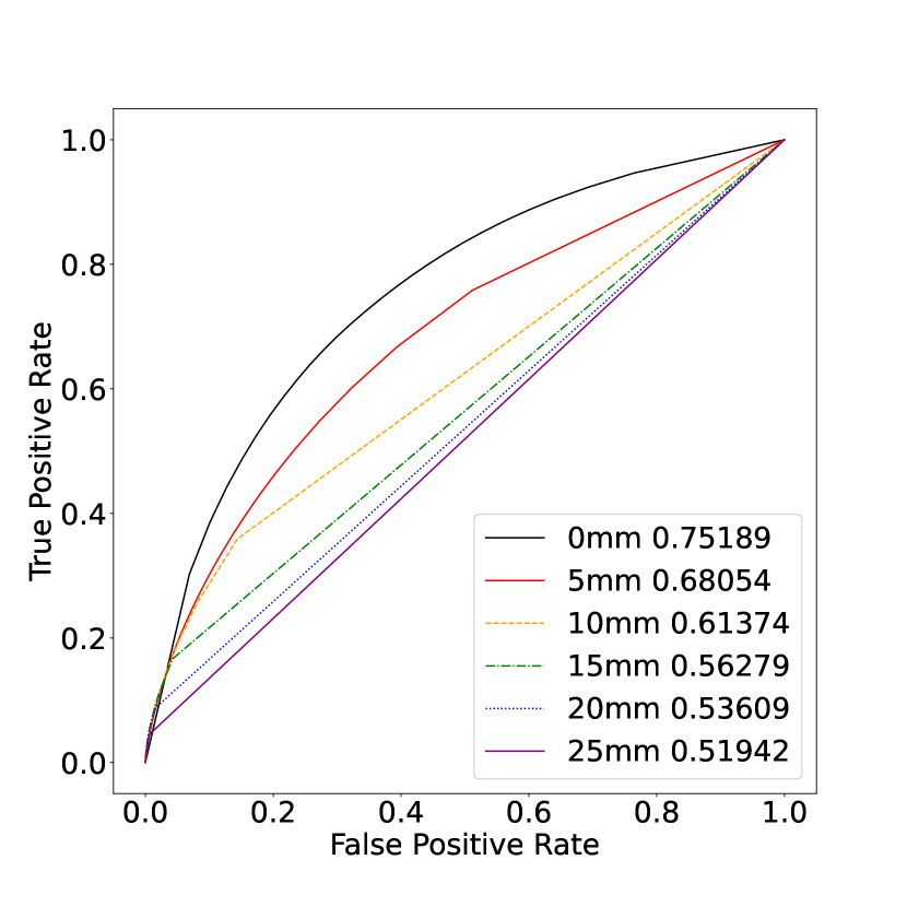
(a) VAE-GAN

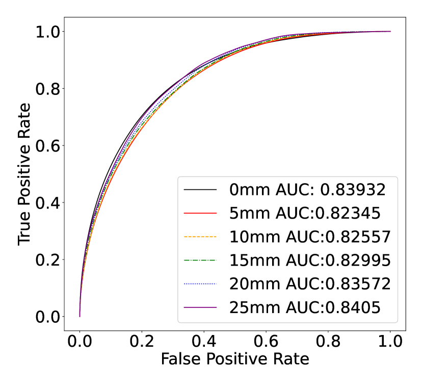
(b) ConvCNP

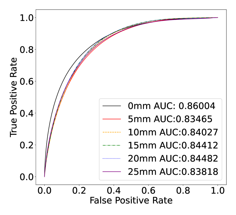
(c) Cens-JGNM

Figure 7: Bechmarking: ROCs for two benchmark methods, namely the (a) the VAE-GAN and (b) ConvCNP as well as our (c) Cens-JGNM approach. Our model demonstrates the best performance, closely matched by the ConvCNP while the VAE-GAN achieves the lowest performance of the three methods.

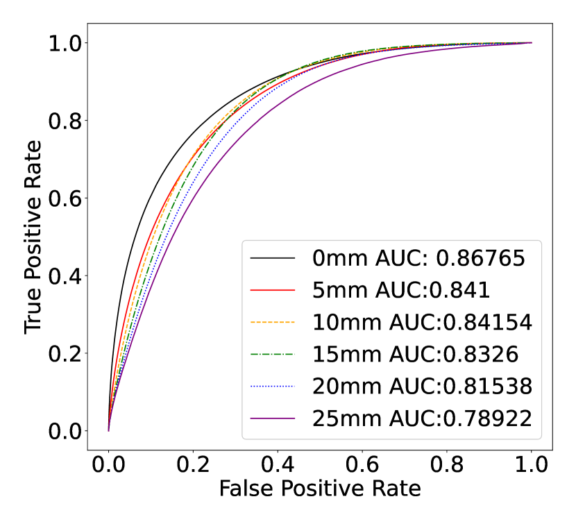
(a) 10 Years

(b) 8 years

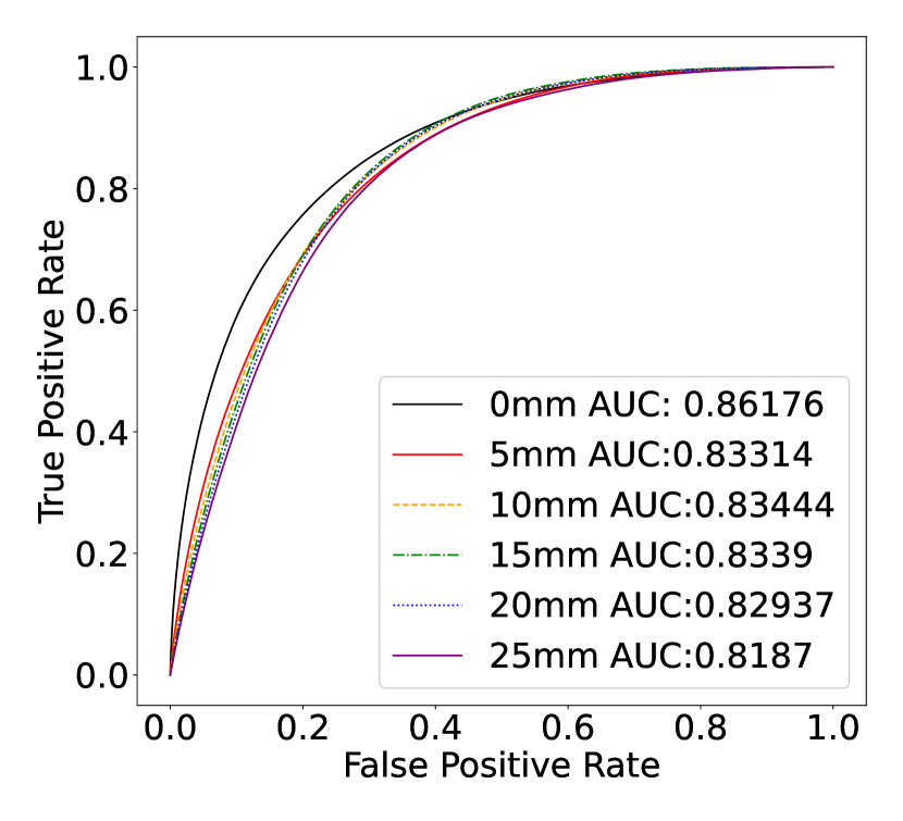
(c) 6 years

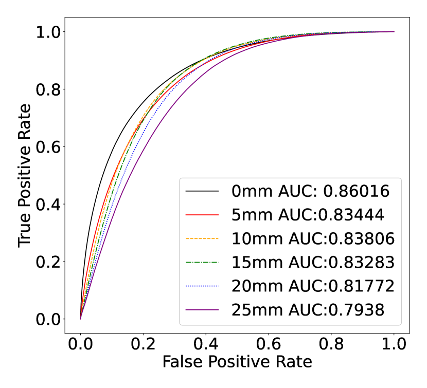
(d) 4 years

Figure 8: Robustness: ROCs for robustness experiments where our Cens-JGNM approach was fitted on (a) 10, (b) 8, (c) 6 and (d) 4 years of data. No clear trend can be noticed, suggesting our approach is robust to any data amount size above four years.

Appendix F Code Reproducibility

The code for the joint generalised neural model can be found at here. Code for all figures shown and for the censored latent Gaussian copula can be found at here.

References

- Adewoyin et al. [2021] R. A. Adewoyin, P. Dueben, P. Watson, Y. He, and R. Dutta. TRU-NET: a deep learning approach to high resolution prediction of rainfall. Machine Learning, 110(8):2035–2062, Jul 2021. ISSN 1573-0565. doi: 10.1007/s10994-021-06022-6. URL http://dx.doi.org/10.1007/s10994-021-06022-6.
- Ailliot et al. [2015] P. Ailliot, D. Allard, V. Monbet, and P. Naveau. Stochastic weather generators: an overview of weather type models. Journal de la société française de statistique, 156(1):101–113, 2015.
- Alquier et al. [2022] P. Alquier, B.-E. Chérief-Abdellatif, A. Derumigny, and J.-D. Fermanian. Estimation of copulas via maximum mean discrepancy. Journal of the American Statistical Association, pages 1–16, 2022.
- Ascenso et al. [2023] G. Ascenso, A. Ficchì, L. Cavicchia, E. Scoccimarro, M. Giuliani, A. Castelletti, et al. Improving the spatial accuracy of extreme tropical cyclone rainfall in ERA5 using deep learning. In EGU General Assembly Conference Abstracts, pages EGU–8085, 2023.
- Behrens et al. [2004] C. N. Behrens, H. F. Lopes, and D. Gamerman. Bayesian analysis of extreme events with threshold estimation. Statistical modelling, 4(3):227–244, 2004.
- Bertolacci et al. [2019] M. Bertolacci, E. Cripps, O. Rosen, J. W. Lau, and S. Cripps. Climate inference on daily rainfall across the Australian continent, 1876–2015. The Annals of Applied Statistics, 13(2):683–712, 2019.
- Chandler [2002] R. Chandler. Glimclim: Generalized linear modelling for daily climate time series (software and user guide). 2002.
- Charles et al. [1999] S. P. Charles, B. C. Bates, and J. P. Hughes. A spatiotemporal model for downscaling precipitation occurrence and amounts. Journal of Geophysical Research: Atmospheres, 104(D24):31657–31669, 1999.
- Chen et al. [2022] J. Chen, T. Janke, F. Steinke, and S. Lerch. Generative machine learning methods for multivariate ensemble post-processing. arXiv preprint arXiv:2211.01345, 2022.
- Chiew et al. [2009] F. Chiew, J. Teng, J. Vaze, D. Post, J. Perraud, D. Kirono, and N. Viney. Estimating climate change impact on runoff across southeast Australia: Method, results, and implications of the modeling method. Water Resources Research, 45(10), 2009.
- Chung et al. [2022] H. C. Chung, I. Gaynanova, and Y. Ni. Phylogenetically informed Bayesian truncated copula graphical models for microbial association networks. The Annals of Applied Statistics, 16(4):2437–2457, 2022.
- Cornes et al. [2019] R. Cornes, G. van der Schrier, E. van den Besselaar, and P. Jones. An ensemble version of the E-OBS temperature and precipitation datasets: version 21.0e, 2019.
- D. Hoff [2007] P. D. Hoff. Extending the rank likelihood for semiparametric copula estimation. 2007.
- Dabernig et al. [2017] M. Dabernig, G. J. Mayr, J. W. Messner, and A. Zeileis. Spatial ensemble post-processing with standardized anomalies. Quarterly Journal of the Royal Meteorological Society, 143(703):909–916, 2017.
- Das [1955] S. Das. The fitting of truncated type III curves to daily rainfall data. Australian Journal of Physics, 8(2):298–304, 1955.
- Dawid et al. [2016] A. P. Dawid, M. Musio, and L. Ventura. Minimum scoring rule inference. Scandinavian Journal of Statistics, 43(1):123–138, 2016.
- Ding et al. [2019] D. Ding, M. Zhang, X. Pan, M. Yang, and X. He. Modeling extreme events in time series prediction. In Proceedings of the 25th ACM SIGKDD International Conference on Knowledge Discovery & Data Mining, pages 1114–1122, 2019.
- Dobra and Lenkoski [2011] A. Dobra and A. Lenkoski. Copula Gaussian graphical models and their application to modeling functional disability data. 2011.
- Dueben and Bauer [2018] P. D. Dueben and P. Bauer. Challenges and design choices for global weather and climate models based on machine learning. Geoscientific Model Development, 11(10):3999–4009, 2018.
- Duncan et al. [2022] J. Duncan, S. Subramanian, and P. Harrington. Generative modeling of high-resolution global precipitation forecasts. arXiv preprint arXiv:2210.12504, 2022.
- Dunn and Smyth [2018] P. K. Dunn and G. K. Smyth. Generalized Linear Models With Examples in R. Springer New York, 2018. doi: 10.1007/978-1-4419-0118-7. URL https://doi.org/10.1007%2F978-1-4419-0118-7.
- Fan et al. [2017] J. Fan, H. Liu, Y. Ning, and H. Zou. High dimensional semiparametric latent graphical model for mixed data. Journal of the Royal Statistical Society. Series B (Statistical Methodology), pages 405–421, 2017.
- Fealy and Sweeney [2007] R. Fealy and J. Sweeney. Statistical downscaling of precipitation for a selection of sites in Ireland employing a generalised linear modelling approach. International Journal of Climatology: A Journal of the Royal Meteorological Society, 27(15):2083–2094, 2007.
- Frost et al. [2011] A. J. Frost, S. P. Charles, B. Timbal, F. H. Chiew, R. Mehrotra, K. C. Nguyen, R. E. Chandler, J. L. McGregor, G. Fu, D. G. Kirono, et al. A comparison of multi-site daily rainfall downscaling techniques under Australian conditions. Journal of Hydrology, 408(1-2):1–18, 2011.
- Gao et al. [2021] J. Gao, P. Ma, J. Du, and X. Huang. Spatial distribution of extreme precipitation in the Tibetan plateau and effects of external forcing factors based on generalized Pareto distribution. Water Supply, 21(3):1253–1262, 2021.
- Gneiting and Raftery [2007] T. Gneiting and A. E. Raftery. Strictly proper scoring rules, prediction, and estimation. Journal of the American Statistical Association, 102(477):359–378, 2007. doi: 10.1198/016214506000001437. URL https://doi.org/10.1198/016214506000001437.
- Gneiting et al. [2005] T. Gneiting, A. E. Raftery, A. H. Westveld, and T. Goldman. Calibrated probabilistic forecasting using ensemble model output statistics and minimum CRPS estimation. Monthly Weather Review, 133(5):1098–1118, 2005.
- Goodfellow et al. [2016] I. Goodfellow, Y. Bengio, and A. Courville. Deep Learning. MIT Press, 2016. http://www.deeplearningbook.org.
- Hamill [2001] T. M. Hamill. Interpretation of rank histograms for verifying ensemble forecasts. Monthly Weather Review, 129(3):550–560, 2001.
- Harris et al. [2022] L. Harris, A. T. T. McRae, M. Chantry, P. D. Dueben, and T. N. Palmer. A generative deep learning approach to stochastic downscaling of precipitation forecasts. Journal of Advances in Modeling Earth Systems, 14(10), oct 2022. doi: 10.1029/2022ms003120. URL https://doi.org/10.1029%2F2022ms003120.
- Hendrycks and Gimpel [2016] D. Hendrycks and K. Gimpel. Gaussian error linear units (GELUs), 2016.
- Hersbach et al. [2020] H. Hersbach, B. Bell, P. Berrisford, S. Hirahara, A. Horányi, and J. Muñoz-Sabater. The ERA5 global reanalysis. Quarterly Journal of the Royal Meteorological Society, 146(730):1999–2049, 2020. doi: 10.1002/qj.3803.
- Holsclaw et al. [2017] T. Holsclaw, A. M. Greene, A. W. Robertson, and P. Smyth. Bayesian nonhomogeneous Markov models via Pólya-gamma data augmentation with applications to rainfall modeling. 2017.
- Huser and Wadsworth [2019] R. Huser and J. L. Wadsworth. Modeling spatial processes with unknown extremal dependence class. Journal of the American Statistical Association, 114(525):434–444, 2019.
- Huser et al. [2016] R. Huser, A. C. Davison, and M. G. Genton. Likelihood estimators for multivariate extremes. Extremes, 19:79–103, 2016.
- Huser et al. [2017] R. Huser, T. Opitz, and E. Thibaud. Bridging asymptotic independence and dependence in spatial extremes using Gaussian scale mixtures. Spatial Statistics, 21:166–186, 2017.
- James P. Hughes and Charles [1999] P. G. James P. Hughes and S. P. Charles. A non-homogeneous hidden Markov model for precipitation occurrence, 1999. URL https://www.jstor.org/stable/2680815.
- Janke et al. [2021] T. Janke, M. Ghanmi, and F. Steinke. Implicit generative copulas. Advances in Neural Information Processing Systems, 34:26028–26039, 2021.
- Jung et al. [2010] T. Jung, G. Balsamo, P. Bechtold, A. Beljaars, M. Koehler, M. Miller, J.-J. Morcrette, A. Orr, M. Rodwell, and A. M. Tompkins. The ECMWF model climate: recent progress through improved physical parametrizations. Quarterly Journal of the Royal Meteorological Society, 136(650):1145–1160, 2010.
- Kirshner [2007] S. Kirshner. Learning with tree-averaged densities and distributions. Advances in Neural Information Processing Systems, 20, 2007.
- Li et al. [2021] R. Li, B. J. Reich, and H. D. Bondell. Deep distribution regression. Computational Statistics & Data Analysis, 159:107203, 2021.
- Li and Smith [2009] Y. Li and I. Smith. A statistical downscaling model for Southern Australia winter rainfall. Journal of Climate, 22(5):1142 – 1158, 2009. doi: 10.1175/2008JCLI2160.1. URL https://journals.ametsoc.org/view/journals/clim/22/5/2008jcli2160.1.xml.
- Little et al. [2008] M. A. Little, P. E. Mcsharry, and J. W. Taylor. Generalised linear models for site-specific density forecasting of UK daily rainfall. 2008. URL http://citeseerx.ist.psu.edu/viewdoc/summary?doi=10.1.1.146.4128.
- MacDonald et al. [2011] A. MacDonald, C. J. Scarrott, D. Lee, B. Darlow, M. Reale, and G. Russell. A flexible extreme value mixture model. Computational Statistics & Data Analysis, 55(6):2137–2157, 2011.
- Matérn [2013] B. Matérn. Spatial variation, volume 36. Springer Science & Business Media, 2013.
- Matheson and Winkler [1976] J. E. Matheson and R. L. Winkler. Scoring rules for continuous probability distributions. Management science, 22(10):1087–1096, 1976.
- McGregor [2005] J. L. McGregor. C-CAM: Geometric aspects and dynamical formulation. Number 70. CSIRO Atmospheric Research Dickson ACT, 2005.
- Mehrotra and Sharma [2007] R. Mehrotra and A. Sharma. Preserving low-frequency variability in generated daily rainfall sequences. Journal of Hydrology, 345(1-2):102–120, 2007.
- Miao et al. [2019] Q. Miao, B. Pan, H. Wang, K. Hsu, and S. Sorooshian. Improving monsoon precipitation prediction using combined convolutional and long short term memory neural network. Water, 11(5):977, 2019.
- Mlakar et al. [2023] P. Mlakar, J. Merše, and J. F. Pucer. Ensemble weather forecast post-processing with a flexible probabilistic neural network approach. arXiv preprint arXiv:2303.17610, 2023.
- Möller and Groß [2016] A. Möller and J. Groß. Probabilistic temperature forecasting based on an ensemble autoregressive modification. Quarterly Journal of the Royal Meteorological Society, 142(696):1385–1394, 2016.
- Möller and Groß [2020] A. Möller and J. Groß. Probabilistic temperature forecasting with a heteroscedastic autoregressive ensemble postprocessing model. Quarterly Journal of the Royal Meteorological Society, 146(726):211–224, 2020.
- Nelder and Lee [1991] J. A. Nelder and Y. Lee. Generalized linear models for the analysis of Taguchi-type experiments. Applied stochastic models and data analysis, 7(1):107–120, 1991.
- Pacchiardi and Dutta [2021] L. Pacchiardi and R. Dutta. Generalized Bayesian likelihood-free inference using scoring rules estimators. arXiv preprint arXiv:2104.03889, 2021.
- Pacchiardi and Dutta [2022a] L. Pacchiardi and R. Dutta. Score matched neural exponential families for likelihood-free inference. Journal of Machine Learning Research, 23(38):1–71, 2022a. URL http://jmlr.org/papers/v23/21-0061.html.
- Pacchiardi and Dutta [2022b] L. Pacchiardi and R. Dutta. Likelihood-free inference with generative neural networks via scoring rule minimization. arXiv preprint arXiv:2205.15784, 2022b.
- Pacchiardi et al. [2022] L. Pacchiardi, R. Adewoyin, P. Dueben, and R. Dutta. Probabilistic forecasting with generative networks via scoring rule minimization, 2022.
- Pan et al. [2019] B. Pan, K. Hsu, A. AghaKouchak, and S. Sorooshian. Improving precipitation estimation using convolutional neural network. Water Resources Research, 55(3):2301–2321, 2019.
- Price and Rasp [2022] I. Price and S. Rasp. Increasing the accuracy and resolution of precipitation forecasts using deep generative models. In International conference on artificial intelligence and statistics, pages 10555–10571. PMLR, 2022.
- Qi et al. [2021] W. Qi, C. Ma, H. Xu, Z. Chen, K. Zhao, and H. Han. A review on applications of urban flood models in flood mitigation strategies. Natural Hazards, 108:31–62, 2021.
- Randall et al. [2007] D. A. Randall, R. A. Wood, S. Bony, R. Colman, T. Fichefet, J. Fyfe, V. Kattsov, A. Pitman, J. Shukla, J. Srinivasan, et al. Climate models and their evaluation. In Climate change 2007: The physical science basis. Contribution of Working Group I to the Fourth Assessment Report of the IPCC (FAR), pages 589–662. Cambridge University Press, 2007.
- Rasmussen et al. [2006] C. E. Rasmussen, C. K. Williams, et al. Gaussian processes for machine learning, volume 1. Springer, 2006.
- Rasp and Lerch [2018] S. Rasp and S. Lerch. Neural networks for postprocessing ensemble weather forecasts. Monthly Weather Review, 146(11):3885–3900, 2018.
- Rasp et al. [2020] S. Rasp, P. D. Dueben, S. Scher, J. A. Weyn, S. Mouatadid, and N. Thuerey. WeatherBench: A benchmark dataset for data-driven weather forecasting, 2020.
- Richards and Wadsworth [2021] J. Richards and J. L. Wadsworth. Spatial deformation for nonstationary extremal dependence. Environmetrics, 32(5):e2671, 2021.
- Richards et al. [2022] J. Richards, J. A. Tawn, and S. Brown. Modelling extremes of spatial aggregates of precipitation using conditional methods. The Annals of Applied Statistics, 16(4):2693–2713, 2022.
- Richards et al. [2023] J. Richards, J. A. Tawn, and S. Brown. Joint estimation of extreme spatially aggregated precipitation at different scales through mixture modelling. Spatial Statistics, page 100725, 2023.
- Scher and Messori [2019] S. Scher and G. Messori. Weather and climate forecasting with neural networks: using general circulation models (GCMs) with different complexity as a study ground. Geoscientific Model Development, 12(7):2797–2809, 2019.
- Schoof [2013] J. T. Schoof. Statistical downscaling in climatology. Geography Compass, 7(4):249–265, 2013.
- Shi et al. [2015] X. Shi, Z. Chen, and H. Wang. Convolutional LSTM network: A machine learning approach for precipitation nowcasting. In Advances in Neural Information Processing Systems 28, pages 802–810. Curran Associates, Inc., 2015.
- Shimizu [1993] K. Shimizu. A bivariate mixed lognormal distribution with an analysis of rainfall data. Journal of Applied Meteorology and Climatology, 32(2):161–171, 1993.
- Sklar [1959] M. Sklar. Fonctions de répartition à n dimensions et leurs marges. In Annales de l’ISUP, volume 8, pages 229–231, 1959.
- Song et al. [2014] Y. Song, Y. Li, B. Bates, and C. K. Wikle. A Bayesian hierarchical downscaling model for south-west Western Australia rainfall. Journal of the Royal Statistical Society Series C: Applied Statistics, 63(5):715–736, 2014.
- Su et al. [2019] H. Su, Z. Xiong, X. Yan, and X. Dai. An evaluation of two statistical downscaling models for downscaling monthly precipitation in the Heihe River basin of China. Theoretical and Applied Climatology, 138:1913–1923, 2019.
- Tareghian and Rasmussen [2013] R. Tareghian and P. Rasmussen. Statistical downscaling of precipitation using quantile regression. Journal of Hydrology, 487:122–135, 04 2013. doi: 10.1016/j.jhydrol.2013.02.029.
- Timbal [2004] B. Timbal. Southwest Australia past and future rainfall trends. Climate Research, 26(3):233–249, 2004.
- Tran et al. [2020] M.-N. Tran, N. Nguyen, D. Nott, and R. Kohn. Bayesian deep net GLM and GLMM. Journal of Computational and Graphical Statistics, 29(1):97–113, 2020. doi: 10.1080/10618600.2019.1637747. URL https://doi.org/10.1080/10618600.2019.1637747.
- Vandal et al. [2017] T. Vandal, E. Kodra, S. Ganguly, A. Michaelis, R. Nemani, and A. R. Ganguly. DeepSD: Generating high resolution climate change projections through single image super-resolution. In Proceedings of the 23rd ACM SIGKDD International Conference on Knowledge Discovery and Data Mining, KDD ’17, page 1663–1672, New York, NY, USA, 2017. Association for Computing Machinery. ISBN 9781450348874. doi: 10.1145/3097983.3098004.
- Vandal et al. [2018] T. Vandal, E. Kodra, J. Dy, S. Ganguly, R. Nemani, and A. R. Ganguly. Quantifying uncertainty in discrete-continuous and skewed data with Bayesian deep learning. Proceedings of the 24th ACM SIGKDD International Conference on Knowledge Discovery and Data Mining, Jul 2018. doi: 10.1145/3219819.3219996.
- Vaughan et al. [2021] A. Vaughan, W. Tebbutt, J. S. Hosking, and R. E. Turner. Convolutional conditional neural processes for local climate downscaling. CoRR, abs/2101.07950, 2021. URL https://arxiv.org/abs/2101.07950.
- Vosper et al. [2023] E. Vosper, P. Watson, L. Harris, A. McRae, R. Santos-Rodriguez, L. Aitchison, and D. Mitchell. Deep learning for downscaling tropical cyclone rainfall to hazard-relevant spatial scales. Journal of Geophysical Research: Atmospheres, page e2022JD038163, 2023.
- Wadsworth and Tawn [2022] J. L. Wadsworth and J. Tawn. Higher-dimensional spatial extremes via single-site conditioning. Spatial Statistics, 51:100677, 2022.
- Wallemacq and Herden [2015] P. Wallemacq and C. Herden. The Human Cost Of Weather Related Disasters. CRED, UNIDSR, 2015.
- Wang et al. [2023] F. Wang, D. Tian, and M. Carroll. Customized deep learning for precipitation bias correction and downscaling. Geoscientific Model Development, 16(2):535–556, 2023.
- Watson et al. [2020] C. D. Watson, C. Wang, T. Lynar, and K. Weldemariam. Investigating two super-resolution methods for downscaling precipitation: ESRGAN and CAR. arXiv preprint arXiv:2012.01233, 2020.
- Watson [2022] P. A. Watson. Machine learning applications for weather and climate need greater focus on extremes. arXiv preprint arXiv:2207.07390, 2022.
- Weyn et al. [2019] J. A. Weyn, D. R. Durran, and R. Caruana. Can machines learn to predict weather? Using deep learning to predict gridded 500-hPa geopotential height from historical weather data. Journal of Advances in Modeling Earth Systems, 11(8):2680–2693, 2019.
- Woo and Wong [2017] W.-C. Woo and W.-K. Wong. Operational application of optical flow techniques to radar-based rainfall nowcasting. Atmosphere, 8(3), 2017. ISSN 2073-4433. doi: 10.3390/atmos8030048.
- Xiang et al. [2022] L. Xiang, J. Xiang, J. Guan, F. Zhang, Y. Zhao, and L. Zhang. A novel reference-based and gradient-guided deep learning model for daily precipitation downscaling. Atmosphere, 13(4):511, 2022.
- Xie et al. [2023] K. Xie, Y. He, J.-S. Kim, S.-K. Yoon, J. Liu, H. Chen, J. H. Lee, X. Zhang, and C.-Y. Xu. Assessment of the joint impact of rainfall characteristics on urban flooding and resilience using the copula method. Water Resources Management, 37(4):1765–1784, 2023.
- Yoon et al. [2020] G. Yoon, R. J. Carroll, and I. Gaynanova. Sparse semiparametric canonical correlation analysis for data of mixed types. Biometrika, 107(3):609–625, 2020.