Asteroseismology and Spectropolarimetry of the Exoplanet Host Star $\lambda$ Serpentis

Abstract

The bright star $\lambda$ Ser hosts a hot Neptune with a minimum mass of 13.6 $M_{\oplus}$ and a 15.5 day orbit. It also appears to be a solar analog, with a mean rotation period of 25.8 days and surface differential rotation very similar to the Sun. We aim to characterize the fundamental properties of this system, and to constrain the evolutionary pathway that led to its present configuration. We detect solar-like oscillations in time series photometry from the Transiting Exoplanet Survey Satellite (TESS), and we derive precise asteroseismic properties from detailed modeling. We obtain new spectropolarimetric data, and we use them to reconstruct the large-scale magnetic field morphology. We reanalyze the complete time series of chromospheric activity measurements from the Mount Wilson Observatory, and we present new X-ray and ultraviolet observations from the Chandra and Hubble space telescopes. Finally, we use the updated observational constraints to assess the rotational history of the star and to estimate the wind braking torque. We conclude that the remaining uncertainty on stellar age currently prevents an unambiguous interpretation of the properties of $\lambda$ Ser, and that the rate of angular momentum loss appears to be higher than for other stars with similar Rossby number. Future asteroseismic observations may help to improve the precision of the stellar age.

The Astronomical Journal

1 Introduction

Asteroseismology and spectropolarimetry are powerful tools to study magnetic stellar evolution. The surface convective regions of Sun-like stars generate sound waves over a broad range of frequencies, some of which are resonant inside the spherical cavity of the star and set up standing waves that produce tiny variations in brightness. These natural oscillations probe the interior conditions of the star, and can be used to infer basic physical properties including the stellar radius, mass, and age (see García & Ballot, 2019). Surface magnetism can break the spherical symmetry of the stellar atmosphere, polarizing the radiated starlight in a way that encodes information about the strength and orientation of the global magnetic field. Multiple snapshot observations of the disk-integrated polarization signature as a star rotates can be used to reconstruct the complete morphology of the large-scale field (see Kochukhov, 2016), which sculpts the escaping stellar wind and influences the rate of angular momentum loss. When combined, these two methods can provide important new constraints on how the magnetic properties of solar-type stars change throughout their lifetimes.

Very few previous studies have combined information from asteroseismic and spectropolarimetric observations. Both techniques require extremely precise measurements, which have only recently become available from space-based photometry (Borucki et al., 2010; Ricker et al., 2014), and ground-based spectropolarimetry (Marsden et al., 2014; Strassmeier et al., 2015). Early efforts relied on observations of massive stars with fossil magnetic fields (Mathis & Neiner, 2015), while more recent work has concentrated on the magnetic evolution of solar-type stars (Metcalfe et al., 2021, 2022, 2023). The latter studies have begun to probe the physical mechanisms that may be responsible for the onset of weakened magnetic braking (van Saders et al., 2016; Hall et al., 2021), revealing a dramatic decrease in the wind braking torque during the second half of main sequence lifetimes. Here we use these techniques to investigate an old main sequence star with some unusual properties.

The exoplanet host star $\lambda$ Ser has been studied for decades as an old solar analog. Long-term observations of its chromospheric emission suggest a nearly constant activity level comparable to recent solar minima (Baliunas et al., 1995), while higher cadence measurements reveal a mean rotation period and surface differential rotation that are both similar to the Sun (Donahue et al., 1996). It has an unusually high lithium abundance for an old solar analog (A(Li)=1.96; Xing & Xing, 2012), with an enhancement comparable to HD 96423 which might be explained by planetary engulfment (Carlos et al., 2016). It was recently confirmed to host a hot Neptune with a minimum mass of 13.6 $M_{\oplus}$ in a 15.5 day orbit (Rosenthal et al., 2021). In this paper, we aim to characterize the properties of $\lambda$ Ser and to constrain the evolutionary pathway that led to its present configuration. In Section 2 we describe new asteroseismic and spectropolarimetric observations, new measurements in the X-ray and ultraviolet, as well as a reanalysis of archival chromospheric activity data. In Section 3 we derive precise stellar properties from asteroseismic modeling, we infer the global magnetic morphology from Zeeman Doppler Imaging (ZDI), and we attempt to interpret these measurements in the context of rotational and magnetic evolution. Finally in Section 4, we discuss possible scenarios to explain the unusual properties of $\lambda$ Ser and we outline future measurements that might clarify its evolutionary status.

2 Observations

2.1 TESS Photometry

The Transiting Exoplanet Survey Satellite (TESS) observed $\lambda$ Ser during Sector 51 (2022 April 22 – 2022 May 18) in 20 s cadence, which has been demonstrated to have superior photometric precision to 2 min data for bright stars (Huber et al., 2022). We were able to improve on the standard Science Processing Operations Center (SPOC) data product by using our own method to extract the light curve (Nielsen et al., 2020). We approached the postage stamp image pixel-by-pixel, extracting a time series for each pixel. We then took the brightest pixel, which was also the closest to the nominal position of the star, as our initial time series. The pixel time series quality figure of merit was parameterized by

$${q=\sum_{i=1}^{N-1}\mid f_{i+1}-f_{i}\mid},$$ (1)

where $f_{i}$ is the flux at cadence $i$, and $N$ is the length of the time series. Using the first differences of the light curve acts to whiten the time series, and thus correct for its non-stationary nature (Nason, 2006); similar approaches have been used in astronomical time series analysis by García et al. (2011), Buzasi et al. (2015), Prša et al. (2019), and Nielsen et al. (2020), among other authors. We then added the light curve from the pixel which most decreased our figure of merit, and repeated the process until the light curve quality as measured by our quality measure $q$ ceased to improve. The resulting pixel collection was adopted as our aperture mask. Finally we detrended the light curve produced using this mask against the centroid pixel coordinates by fitting a second-order polynomial with cross terms. Similar approaches have been used for K2 data reduction (e.g., see Vanderburg & Johnson, 2014).

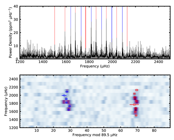
Figure 1: Power spectrum (top) and échelle diagram (bottom) centered on the power excess due to solar-like oscillations detected in $\lambda$ Ser. Blue solid lines and circles indicate extracted radial ($l=0$) modes, while red dashed lines and squares show extracted dipole ($l=1$) modes.

The overall noise level of our light curve, measured point-to-point, is approximately 7% better than that of the SPOC product, and we were able to recover more points: 67,491 as compared to 55,445 in the SPOC light curve (or 58,528 if requirements are relaxed to include points with nonzero quality flags). This improved the duty cycle from 52-55% to almost 64%. The top panel of Figure 1 shows the power spectrum of the resulting time series with clear evidence for solar-like oscillations centered near 1900 $\mu$Hz. We use this same approach in Appendix A to quantify non-detections of oscillations in eight additional TESS targets.

To extract individual frequencies, four different groups of coauthors applied either iterative sine-wave fitting (e.g. Lenz & Breger, 2005; Kjeldsen et al., 2005; Bedding et al., 2007) or Lorentzian mode-profile fitting (e.g. García et al., 2009; Handberg & Campante, 2011; Appourchaux et al., 2012; Mosser et al., 2012; Corsaro & De Ridder, 2014; Corsaro et al., 2015; Li et al., 2020; Breton et al., 2022). For each mode, we required at least two independent methods to return the same frequency within uncertainties. For the final list we adopted values from a single method, with uncertainties derived by adding in quadrature the median formal uncertainty and the standard deviation of the extracted frequencies from all methods that identified a given mode.

The bottom panel of Figure 1 shows an échelle diagram with a large separation of $\Delta\nu=89.5$ $\mu$Hz and the extracted frequencies. We identify six radial ($l=0$) and eight dipole ($l=1$) modes, but we were unable to identify any quadrupole ($l=2$) modes with confidence. Mode identification was confirmed using well-known patterns between $\Delta\nu$ and the frequency offset $\epsilon$ (White et al., 2011) and by comparison with similar stars (e.g., KIC 7296438) from the Kepler LEGACY sample (Lund et al., 2017). The final frequency list is shown in Table 1, providing a primary input for the asteroseismic modeling described in Section 3.1.

2.2 Spectropolarimetry

Table 1: Identified oscillation frequencies for $\lambda$ Ser.

$l$	$\nu~{}(\mbox{$\mu$Hz})$	$\sigma_{\nu}~{}(\mbox{$\mu$Hz})$
0	1640.04	0.42
0	1730.13	0.74
0	1817.79	0.61
0	1907.18	0.77
0	1995.41	1.48
0	2086.52	0.85
1	1501.22	0.74
1	1590.24	0.50
1	1679.97	0.32
1	1768.62	2.72
1	1859.28	0.60
1	1947.86	0.42
1	2037.22	0.52
1	2128.08	0.94

Spectropolarimetric observations of $\lambda$ Ser were obtained on 2021 May 24 using the Potsdam Echelle Polarimetric and Spectroscopic Instrument (PEPSI; Strassmeier et al., 2015) installed at the $2\times 8.4$-m Large Binocular Telescope (LBT). The instrumental setup, resulting in $R$ = 130,000 observations over the 475–540 nm and 623–743 nm wavelength regions, and the data reduction procedures were the same as described in Metcalfe et al. (2019). Considering the low-amplitude polarization signal, a multi-line method is necessary to achieve a magnetic field detection. Here we employed the least-squares deconvolution (LSD; Kochukhov et al., 2010) technique to derive high-quality intensity and circular polarization profiles. The line mask necessary for this analysis was constructed from the output of an “extract stellar” request to the VALD database (Ryabchikova et al., 2015) with stellar atmospheric parameters from Brewer et al. (2016). This line list contained 1300 metal lines deeper than 10% of the continuum in the wavelength region covered by our PEPSI data. Combining information from these lines yielded an LSD Stokes $V$ profile with an uncertainty of 4.6 ppm, which showed a clear magnetic signal (see Figure 2). We measured a mean longitudinal magnetic field $\left<B_{\rm z}\right>=0.674\pm 0.048$ G from these observations and estimated the strength of an axisymmetric dipole magnetic field to be $B_{\rm d}=3.8$ G using the line profile modeling technique described in Metcalfe et al. (2019) and adopting $i=50\arcdeg$ (see Section 3.2). However, the resulting synthetic profile (dotted red line in Figure 2) did not provide an adequate description of the observations, suggesting the presence of non-axisymmetric global field components. Consequently, we generalized the modeling by allowing an inclined dipole geometry. This produced a better fit to the observed Stokes $V$ profile with $B_{\rm d}=6.0$ G and a magnetic obliquity of $\beta=51.5\arcdeg$ (dashed blue line in Figure 2).

Additional spectropolarimetric observations of $\lambda$ Ser covering a broad range of rotation phases were collected with Neo-NARVAL during the summer of 2021, allowing us to model the detailed morphology of its large-scale magnetic field. The complete data set included 19 visits to the star, secured between 2021 July 7 and 2021 August 17, with a maximum of one observation per night. Neo-NARVAL is an upgrade to the NARVAL instrument at Télescope Bernard Lyot (TBL; Aurière, 2003). Neo-NARVAL echelle spectra collect a broad optical wavelength region (370–1,000 nm) in a single frame, with a spectral resolution close to $R$ = 65,000. Every polarimetric sequence is obtained from the combination of four exposures taken with the two half-wave Fresnel rhombs rotated about the optical axis (Semel et al., 1993). Each polarized sequence provides simultaneous access to a Stokes $I$ spectrum and another Stokes parameter (circular or linear polarization). The data set gathered for $\lambda$ Ser was restricted to the Stokes $V$ parameter, since the amplitude of Zeeman signatures is expected to be largest in circular polarization (Landi Degl’Innocenti, 1992). Each sequence also provides a “null” spectrum, which should contain only noise and serves as a diagnostic of possible instrumental or stellar contamination to the polarized spectrum.

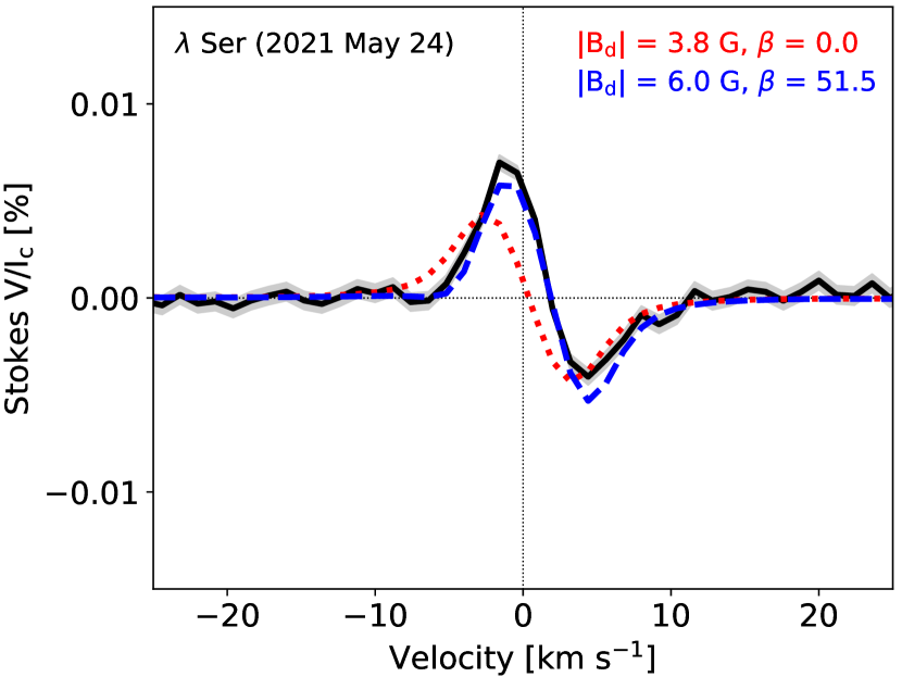
Figure 2: Stokes $V$ polarization profile for $\lambda$ Ser from LBT observations on 2021 May 24. The mean profile is shown as a black line, with uncertainties indicated by the gray shaded area. The red and blue lines are model profiles assuming dipole geometry and fixed inclination $i=50^{\circ}$ with different obliquity angles $\beta$.

The Neo-NARVAL upgrade, installed in 2019, consisted of a new detector and enhanced velocimetric capabilities (López Ariste et al., 2022). At the time of our observations, the instrument suffered from a loss of flux in the bluest orders, later identified as a fiber link issue. The new reduction pipeline (López Ariste et al., 2022) provided an unsatisfactory extraction of spectral orders affected by a very low signal-to-noise ratio (S/N), so we discarded from our reduced data all spectral bins with a wavelength below 470 nm. The LSD analysis and interpretation of these data are described in Section 3.2.

2.3 X-Ray Measurements

We observed $\lambda$ Ser with the Chandra High Resolution Camera-Imaging detector (HRC-I; ObsID 22307) on 2020 April 25 in a single pointing with a net exposure time of 6,103 s. This instrument was preferred over the Advanced CCD Imaging Spectrometer (ACIS) because a growing contamination layer on the ACIS optical blocking filter severely curtails the low-energy response below about 1 keV. The HRC-I data were reprocessed using the Chandra Interactive Analysis of Observations (CIAO; Fruscione et al., 2006) software version 4.15 and calibration database version 4.10.2. Since the HRC-I has essentially no intrinsic energy resolution, the analysis entailed examining the source photon event list for significant variability, extracting photon events attributed to $\lambda$ Ser, and converting the observed count rate into a source flux.

An image of the detected events in the vicinity of $\lambda$ Ser is shown in Figure 3. Overlaid is the adopted source extraction region (yellow), together with the innermost of two background regions (cyan) employed to estimate the background signal. The source region was placed at the centroid of the detected events and had a radius of 1.5″, which corresponds to an encircled energy fraction of 95%. The background region illustrated in Figure 3 was an annulus with inner and outer radii of 3.5″and 7″, respectively, centered on the source. We also estimated the background rate using a much larger annulus, covering the radius interval 130″–165″, to check for the presence of spatial variations in the background. In both cases the net source count rate was $0.049\pm 0.003$ count s^-1 after correction for the encircled energy fraction. The extracted source counts were examined for variability using the Gregory-Loredo algorithm (Gregory & Loredo, 1992); no significant variability was detected.

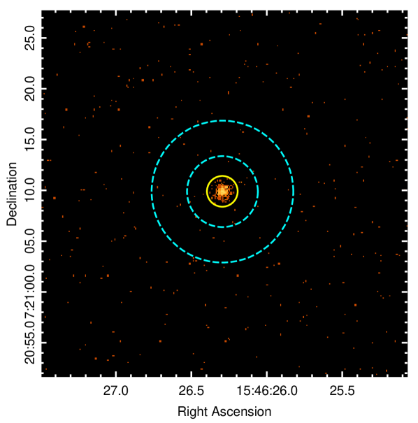
Figure 3: Chandra HRC-I image of $\lambda$ Ser illustrating the source and innermost of two background regions used for the count rate measurement (see Section 2.3 for details).

In addition to the Chandra observation, $\lambda$ Ser was observed in soft X-rays during the ROSAT era, initially as part of the all-sky survey (scans were acquired in 1990 August), and later during the pointed phase of the Guest Investigator program (a PSPCB exposure in 1997 February, toward the end of the mission). Count rates (CR) for the two ROSAT observations were taken from facility catalogs hosted by the High-Energy Science and Archive Research Center (HEASARC), at the NASA Goddard Space Flight Center, as accessed through W3browse. The rass2rxs catalog listed CR = $0.083\pm 0.016$ count s^-1 for a sky survey exposure of 511 s. The pointings catalog rospspctotal reported CR = $0.072\pm 0.006$ count s^-1 for an exposure of 2.73 ks. The energy bandpass is the ROSAT standard, 0.1–2.4 keV. Documentation for these databases can be obtained through W3browse.

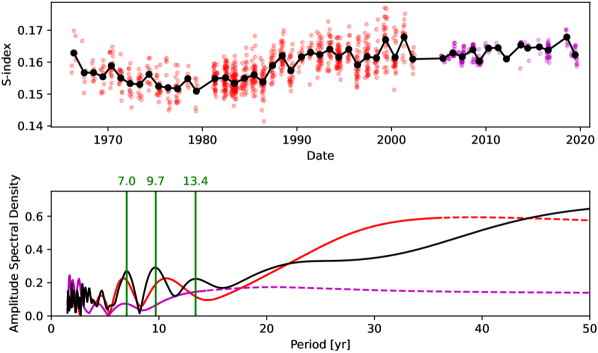
Figure 4: Top: 54-year $S$-index time series for $\lambda$ Ser. Observations are shown from MWO HKP (red) and Keck HIRES-2 (purple) with seasonal means (black). Bottom: Lomb-Scargle periodogram of the time series, with MWO-only in red, Keck-only in purple, and the composite time series in black. Dashed lines indicate portions of the periodogram beyond the duration of the time series. The top three peaks in the composite time series are indicated with green vertical lines. The periodogram is expressed in units of signal amplitude normalized by a standard deviation.

The count rates from ROSAT and Chandra were converted to X-ray fluxes at Earth using a method to derive an optimum energy conversion factor (ECF) for each camera system. The approach applied a sequence of coronal emission-measure distributions (EMD), convolved with detector-dependent sensitivity curves, to calculate X-ray surface fluxes for the target; finding the optimum EMD realization that achieved consistency between the calculated and model surface fluxes (each EMD level corresponds to a specific predicted X-ray surface flux). The approach is described by Ayres & Buzasi (2022), and is based on the empirical EMD models derived by Wood et al. (2018) from Chandra Low-Energy Transmission Grating spectra of nearly two dozen F–M dwarfs. Detector sensitivity curves were calculated for the reference $\log{T}$ grid of each EMD using WebPIMMS, for the unabsorbed 0.1–2.4 keV X-ray flux, a solar-abundance APEC plasma model, and an interstellar column of $1{\times}10^{18}$ cm^-2, appropriate for a nearby ($d=11.9$ pc) star. There was good consistency among the three independent X-ray fluxes: $f_{\rm X}=4.0\pm 0.4{\times}10^{-13}$ erg cm^-2 s^-1. At the Gaia distance, this corresponds to $L_{\rm X}=6.8\pm 0.6{\times}10^{27}$ erg s^-1, or $\log{L_{\rm X}}$ = 27.83, about seven times larger than the sunspot-cycle-average Sun (Ayres & Buzasi, 2022).

We can estimate the mass-loss rate of $\lambda$ Ser by combining the X-ray luminosity determined above with the stellar radius inferred from asteroseismology (see Section 3.1). For stars with mass-loss rates determined directly from Ly$\alpha$ measurements and other techniques, there is an empirical relation between the mass-loss rate and the X-ray flux per unit surface area, $\dot{M}\propto F_{\rm X}^{0.77}$ (Wood et al., 2021). The resulting estimate is slightly above the solar value, $\dot{M}=1.6\pm 0.2\ \dot{M}_{\odot}$.

2.4 Chromospheric Activity Data

We used synoptic observations of the $S$-index of chromospheric activity from the Mount Wilson Observatory (MWO) HK Project (Wilson, 1978; Baliunas et al., 1996) and the Keck HIRES spectrometer (Baum et al., 2022) to measure the rotation period of $\lambda$ Ser and to characterize its long-term magnetic variability. The $S$-index was defined by the MWO HK Photometer (HKP) and measured the ratio of emission from 0.1 nm cores of the chromospheric Ca ii H & K lines to the sum of two nearby 2 nm pseudo-continuum bandpasses (Vaughan et al., 1978). This long-used proxy for stellar magnetic activity reveals the presence of decadal-scale cycles in the Sun (e.g. White & Livingston, 1981; Egeland et al., 2017) and Sun-like stars (e.g. Baliunas et al., 1995; Hall et al., 2007; Egeland, 2017). The passage of surface active regions modulates the $S$-index such that when sampled at a sufficient cadence the stellar rotation period can be obtained (Baliunas et al., 1983, 1996; Donahue et al., 1996). The MWO HK Project observed $\lambda$ Ser from its inception in 1966 until its termination in 2003. Previous studies have reported results on partial records of $\lambda$ Ser, but here we analyze the complete time series obtained by MWO.

Table 2: Seasonal Rotation Period Detections for $\lambda$ Ser

	Donahue				This Work
Season	$N_{\rm obs}$	$P_{\rm rot}$	$\Delta P$	FAP	$N_{\rm JD}$	$P_{\rm rot}$	$\sigma_{P}$	FAP
1970.36					21	19.4	0.7	3.01%
1977.36					24	23.0	0.5	0.56%
1981.34	103	24.4	0.2	0.0015%	35	25.5	0.5	0.003%
1983.38	271	27.1	0.3	3.4%
1986.40	124	28.8	0.4	0.20%	42	28.0	1.3	2.97%
1987.41	84	24.3	0.3	2.1%
1988.45	113	26.4	0.4	0.12%	37	26.3	0.6	2.59%
1992.42	91	23.6	0.4	1.5%	39	23.3	0.2	0.04%
N detections		6				6
Min $P_{\rm rot}$		23.6				19.4
Max $P_{\rm rot}$		28.8				28.0
Mean $P_{\rm rot}$		25.8				24.3

Note. — Donahue values are taken from Table B.25 of Donahue (1993). The decimal year in the Season column gives the mean decimal year of the observations in that season. $N_{\rm obs}$ refers to the individual MWO observations analyzed by Donahue, while $N_{\rm JD}$ refers to the nightly (Julian Day) averages used in this work.

We extend the MWO observations using Keck Observatory HIRES-2 data obtained for the California Planet Search (CPS) and published in Baum et al. (2022). These High Resolution Echelle Spectrometer (HIRES) observations (R $\sim$ 67,000) cover the Ca ii H & K region, and the $S$-index is obtained by reducing the spectra and integrating the bandpasses of the MWO HKP-2 spectrophotometer (Vaughan et al., 1978; Isaacson & Fischer, 2010). While some data from Baum et al. (2022) were adjusted with a constant shift to be consistent with MWO, no such shift was applied to the data set for $\lambda$ Ser. The composite data set is shown in the top panel of Figure 4 with the seasonal means indicated. Some low-frequency variation is apparent by visual inspection of the seasonal means. Activity falls from the beginning of the observations in 1966 ($S=0.1629$) until the global minimum seasonal mean in 1979 ($S=0.1509$). From there, activity rises until about 1988 ($S=0.1620$) and remains relatively constant thereafter. The global maximum seasonal mean occurs in 2001 ($S=0.1679$), but this appears to be an intermittent outburst reaching levels comparable to 1999 and 2018. The standard deviation of the seasonal means including and after the 1988 season is $\sigma_{S}=0.00236$ ($N=29$), which is about half of the standard deviation for the whole series ($\sigma_{S}=0.00460,N=50$). For reference, solar minimum has $S=0.1621$ and the mean cycle maximum is $S=0.177$ (Egeland et al., 2017).

We employed the Lomb-Scargle periodogram (Lomb, 1976; Scargle, 1982; Horne & Baliunas, 1986) to search for periodicity in the separate (MWO, Keck) and composite time series. A Monte Carlo of 100,000 trials was used, drawing from a Gaussian distribution with the same variance as the data and using the original sampling, to determine the periodogram power threshold level for a 0.1% false alarm probability (FAP)—i.e., the probability that a periodogram peak could be generated by Gaussian noise. Peaks above this level are considered significant and were ranked in order of decreasing power. From the MWO time series, with a duration of 36.3 years, the top three significant peaks are found at 39.1, 6.7, and 10.7 years, and the remaining four significant peaks have periods less than 3.5 years. While the Lomb-Scargle periodogram method is capable of detecting harmonic periodicity that extends beyond the duration of the data, such low frequency peaks in a more complex time series can be a result of the data window, and must be viewed with extreme caution. From the Keck HIRES-2 time series, with a duration of 14.3 years, no significant low frequency periods are detected within the data window, and a peak of 20.5 years is found beyond it. Finally, from the composite dataset significant peaks are found at $9.65\pm 0.09$, $7.00\pm 0.05$, and $13.4\pm 0.2$ years, the first two corresponding well to the MWO-alone time series. These results compare well to the Egeland (2017) study that combined the MWO data with observations from the Lowell Observatory Solar Stellar Spectrograph (SSS), where peaks of 43.3, 6.7, and 12.8 years were found. In that study, the long period peak was viewed with skepticism due to a step discontinuity in the SSS data corresponding to a CCD upgrade in the SSS. The HIRES-2 data does not suffer from such a discontinuity, and the power at low frequencies from the composite dataset is diminished, indicating that the $\sim$40 year “cycle” indicated by the MWO data alone is not supported by these extended observations. Variability on the scale of $\sim$7 to $\sim$13 years is the most prominent and reliable, however the variations in $\lambda$ Ser are not as clean and Sun-like as the solar-cycle and the term “cycle” for these periodicities should be applied with caution, as discussed more generally in Egeland (2017). The periodogram in Figure 4 is expressed in units of normalized amplitude $A_{N}=\sqrt{2P_{N}/N}$, where $P_{N}$ is the usual periodogram power normalized by the variance. This normalization is useful for comparing time series of different lengths and judging cycle quality as it: (1) is independent of the number of observations, (2) has a maximum value of 1, and (3) is a relative measure of signal purity for a given peak (see discussion in Egeland, 2017).

Individual seasons of the MWO and Keck time series with more than 20 observations were analyzed to search for rotational modulation, following previous efforts by Donahue (1993) and Donahue et al. (1996). As with the cycle search, a Lomb-Scargle periodogram was employed using a 100,000 trial Monte Carlo to determine the power threshold for a 5% FAP. For a search range between 10 and 40 days, peaks above the 5% FAP threshold are reported as seasonal rotation periods. When significant peaks were found, a 100,000 trial periodogram Monte Carlo was used, adjusting the observations within their errors to determine the period uncertainty. We compare our results to the previous work of Donahue (1993) in Table 2. Our analysis largely confirms the earlier results, which found rotation signals in six seasons ranging from 23.6 to 28.8 days. We also find significant periods in six seasons, though not the same six found by Donahue, with rotation ranging from 19.4 days to 28.0 days. The differences may be ascribed to: (1) Donahue analyzed individual $S$-index observations, while we used a nightly average from typically three observations per night, (2) the MWO time series were recalibrated after Donahue’s work, and (3) different observation rejection criteria were employed. No significant rotation periods were found in the lower-cadence MWO data beyond the 1993 season, which were not analyzed by Donahue (1993), nor in the Keck HIRES-2 data. The Keck observations tend to be clustered around a few dates within a season, making them unsuitable for a rotation period search.

To summarize, our analysis of the composite MWO and Keck $S$-index time series indicates a mean rotation period of $24.3\pm 2.7$ days, with strong indications of differential rotation, $({\rm max}(P_{\rm rot})-{\rm min}(P_{\rm rot}))/{\rm min}(P_{\rm rot})=44\%$. Significant long-term variability at 9.7, 7.0, and 13.4 years was found, but it does not appear to be dominated by a single period that would indicate a “clean” cycle as for the Sun. A large amplitude long-period variation of approximately 40 years is apparent in the MWO data, but the 54-year composite dataset does not support this periodicity being cyclic. Extended uniform data sets are required to determine whether such long-period cycles exist in $\lambda$ Ser or other stars.

2.5 Spectral Energy Distribution

As an independent determination of the stellar properties, we performed an analysis of the broadband spectral energy distribution (SED) of $\lambda$ Ser and the Gaia DR3 parallax (with no systematic offset applied; see, e.g., Stassun & Torres, 2021), to derive an empirical measurement of the stellar radius, following the procedures described in Stassun & Torres (2016); Stassun et al. (2017) and Stassun et al. (2018). We adopted the $UBV$ magnitudes from Mermilliod (2006), the $B_{T}V_{T}$ magnitudes from Tycho-2, the Strömgren $ubvy$ magnitudes from Paunzen (2015), the $JHK_{S}$ magnitudes from 2MASS, the W1–W4 magnitudes from WISE, the $G_{\rm BP}G_{\rm RP}$ magnitudes from Gaia, and the FUV magnitude from GALEX. Together, the available photometry spans the full stellar SED over the wavelength range 0.2–22 $\mu$m.

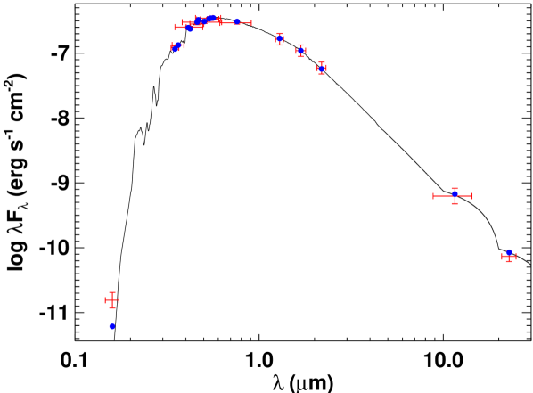
Figure 5: Spectral energy distribution of $\lambda$ Ser. Red symbols represent the observed photometric measurements, where the horizontal bars represent the effective width of the passband. Blue symbols are the model fluxes from the best-fit Kurucz atmosphere model (black).

We performed a fit using Kurucz stellar atmosphere models, with the effective temperature ($T_{\rm eff}$), surface gravity ($\log g$), and metallicity ([M/H]) from Brewer et al. (2016), with uncertainties inflated to account for a realistic systematic noise floor. The remaining free parameter is the extinction $A_{V}$, which we fixed at zero due to the star’s proximity ($d=11.9$ pc). The resulting fit (Figure 5) has a reduced $\chi^{2}$ of 1.1, excluding the GALEX FUV flux which indicates a moderate level of activity. Integrating the (unreddened) model SED gives the bolometric flux at Earth, $F_{\rm bol}=4.481\pm 0.052\times 10^{-7}$ erg s^-1 cm^-2. Taking the $F_{\rm bol}$ together with the Gaia parallax gives the bolometric luminosity, $L_{\rm bol}=1.984\pm 0.023\ L_{\odot}$, which together with $T_{\rm eff}$ gives the stellar radius, $R=1.349\pm 0.024\ R_{\odot}$. In addition, we can estimate the stellar mass from the empirical relations of Torres et al. (2010), giving $M=1.17\pm 0.07\ M_{\odot}$, which is consistent with that obtained directly from R and $\log g$ ($M=1.11\pm 0.12\ M_{\odot}$). These estimates of the radius and mass can be compared to the adopted values from asteroseismology in Section 3.1.

2.6 Hubble Space Telescope Data

Table 3: Measured FUV Line Fluxes for $\lambda$ Ser

Ion(s)	Wavelength	Flux at Earth
	[Å]	[10-15 ergs cm-2 s-1]
C iii1	1175	29.3 $\pm$ 1.3
Si iii1	1198	0.27 $\pm$ 0.19
O i1	1304	54.8 $\pm$ 1.1
C ii1	1335	71.3 $\pm$ 0.9
Cl i2	1351.7	2.2 $\pm$ 0.3
Si iv	1393.8	27.3 $\pm$ 0.7
O iv	1399.8	1.3 $\pm$ 0.3
O iv	1401.2	1.9 $\pm$ 0.3
Si iv2	1402.8	12.44 $\pm$ 0.6
Si iv+O iv2	1404.8	2.40 $\pm$ 0.6
O iv2	1407.4	0.30 $\pm$ 0.16
N iv	1486.3	1.2 $\pm$ 0.3
Continuum3	1506	21.4 $\pm$ 0.8
Si ii	1526.5	8.9 $\pm$ 0.9
Si ii	1533.7	8.4 $\pm$ 0.8
C iv2	1548	40.2 $\pm$ 1.3
C iv2	1550	18.2 $\pm$ 1.1
C i1,2	1561	13.5 $\pm$ 1.0
He ii	1640.7	17.5 $\pm$ 1.5
C i1	1657	62.7 $\pm$ 2.5
O iii	1666.2	2.4 $\pm$ 1.2
Si ii	1808.0	26.9 $\pm$ 3.1
Si ii	1817.1	138 $\pm$ 5
Al iii	1854.6	10.3 $\pm$ 3.6
Si iii	1892.0	88.4 $\pm$ 6.6
C iii	1908.7	50.8 $\pm$ 7.9

Note. — All fluxes are from direct integration, except ¹Multiple lines combined, ²Voigt function fitting and deblending, ${}^{3}\pm$5 Å integration of a largely line-free region.

As a probe of the physical environment between the photosphere and the corona, we also observed $\lambda$ Ser using the Cosmic Origins Spectrograph (COS) on the Hubble Space Telescope (HST). We obtained a low resolution G140L FUV spectrum with an integration time of 1976 s on 2020 September 2 (program 15991), which was reduced with standard pipeline processing. We computed integrated fluxes for isolated emission lines in the rest frame of the star above nearby pseudo-continua, together with RMS errors. We estimated continua from linear fits to clusters of low points on either side of the line in question. When the target line was blended, two methods were employed. Some weaker blends were removed by fitting a Voigt function to better mimic the convolved instrumental profile and line shape, leaving the residual target line for flux integration as before. In some cases, we fit the entire complex of lines with multiple Voigt functions. The results are shown in Table 3. Tests on isolated lines demonstrated that straight integration and Voigt fitting yielded similar results, typically within $\pm$5%. In several cases, multiple nearby lines of the same ion were combined. Following Ayres (2020), we also measured a 10 Å segment of relatively line-free FUV pseudo-continuum centered at 1506 Å.

Table 4: Comparison of FUV Surface Fluxes

Ion(s)	Wavelength	Surface Flux [103 ergs cm-2 s-1]
	[Å]	$\lambda$ Ser	Sun2	$\alpha$ Cen A2
C iii1	1175	4400 $\pm$ 200	2250	$\cdots$
O i1	1304	8230 $\pm$ 160	5490	5800 $\pm$ 290
C ii1	1335	10700 $\pm$ 140	7000	7000 $\pm$ 350
Cl i	1351.7	330 $\pm$ 43	252	$\cdots$
Si iv	1393.8	4110 $\pm$ 104	1690	3200 $\pm$ 1601
Si iv	1402.8	1870 $\pm$ 86	875	$\cdots$
Continuum	1506	3210 $\pm$ 117	1780	$\cdots$
C iv	1548	6030 $\pm$ 198	3800	6200 $\pm$ 3101
C iv	1550	2730 $\pm$ 171	1960	$\cdots$

Note. — ¹Multiple lines combined, ²Results from Ayres (2020).

We can compare the FUV fluxes of $\lambda$ Ser to the Sun and to $\alpha$ Cen A, a somewhat older (5.3 Gyr; Joyce & Chaboyer, 2018), more metal rich (Fe/H=+0.24; Morel, 2018) solar analog (see Table 4). Lower chromospheric surface fluxes in Cl i and O i (with temperatures of peak emissivity $\log T_{\rm peak}$ = 3.8–3.9) are 1.3 to 1.5 times larger in $\lambda$ Ser; the upper chromospheric C ii flux ($\log T_{\rm peak}=4.5$) is similarly $\approx 1.5\times$ enhanced. Moving to lines formed in the stellar transition region, C iii ($\log T_{\rm peak}=4.8$) is $\approx 2\times$ enhanced in $\lambda$ Ser relative to the Sun, Si iv ($\log T_{\rm peak}$ = 4.9) is further enhanced, at a factor of 2.3 and 1.9 relative to the Sun and $\alpha$ Cen A, respectively (the higher metallicity of $\alpha$ Cen A may boost its emission). In the C iv doublet ($\log T_{\rm peak}$ = 5.0), the enhancement in $\lambda$ Ser returns to a factor of $\approx$1.5 (here some optical depth effects may play a role). These results are generally in line with the more active corona of $\lambda$ Ser—which shows 3.8$\times$ the solar surface $F_{X}$—and with the reduced activity enhancements relative to the corona that are expected for lower $T_{\rm peak}$ emission in the chromosphere and transition region (e.g., Ayres & Buzasi, 2022, among many).

Several density-sensitive line ratios are available in the HST spectra. We use the intersection of these results to estimate the electron density in the transition region. The Si iii(1892 Å)/C iii(1909 Å) ratio, with $\log T_{\rm peak}\sim 4.7$, yields $\log n_{e}=9.87_{-0.18}^{+0.08}$ using Keenan et al. (1987). The ratio C iii(1908 Å)/Si iv(1402 Å), with $\log T_{\rm peak}\sim 4.8$, gives $\log n_{e}=9.98_{-0.06}^{+0.05}$. The ratios O iii(1666 Å)/Si iv(1402 Å) and C iii(1908 Å)/O iii(1666 Å), also with $\log T_{\rm peak}\sim 4.8$, were less certain, affected by larger errors in the O iii line; these yield $\log n_{e}=10.80_{-0.41}^{+0.40}$ and $9.76_{-1.44}^{+0.30}$, respectively (using Keenan et al., 1988). Another $\log T_{\rm peak}\sim 4.8$ diagnostic, C iii(1908 Å)/Al iii(1863 Å), implies $\log n_{e}=10.24_{-0.21}^{+0.21}$ (employing Keenan et al., 1990). A hotter diagnostic, the ratio O iv(1401 Å)/O iv(1407 Å) at $\log T_{\rm peak}\sim 5.1$ (using results of Brage et al., 1996) unfortunately gives only a weak limit of $\log n_{e}<10.3$ due to large errors on the fluxes. Combining the cooler diagnostics, we find an average $\langle\log n_{e}\rangle=10.06_{-0.06}^{+0.05}$ at $\log T_{\rm peak}\sim 4.8$. For comparison, $\langle\log n_{e}\rangle=10.0$ using the hotter O iv ratio in the Sun (e.g., Rao et al., 2022). This suggests that $\lambda$ Ser has transition region densities similar to, or perhaps slightly lower than, the Sun at fixed temperature, which is consistent with its slightly lower surface gravity. We caution, however, that assumptions intrinsic to the line ratio method make the results uncertain (see discussion in Judge, 2020).

In summary, $\lambda$ Ser has chromospheric and transition region fluxes broadly consistent with a star which is somewhat more coronally active, and has slightly lower density than the Sun.

3 Interpretation

3.1 Asteroseismic Modeling

Using the oscillation frequencies listed in Table 1, spectroscopic constraints on $T_{\rm eff}$ and $\mathrm{[M/H]}$ from Brewer et al. (2016), and the luminosity from Section 2.5, five teams attempted to infer the properties of $\lambda$ Ser from asteroseismic modeling. A variety of stellar evolution codes and fitting methods were employed, including ASTEC (AMP) (Christensen-Dalsgaard, 2008; Metcalfe et al., 2009), GARSTEC (BASTA) (Weiss et al., 2008; Aguirre Børsen-Koch et al., 2022), MESA (Paxton et al., 2015; Li et al., 2023), and YREC (Demarque et al., 2008). We found reasonable agreement between the results for the stellar radius and mass, with individual estimates ranging from $R=1.33$–1.38 $R_{\odot}$ and $M=1.03$–1.13 $M_{\odot}$, but there was a significant spread in stellar age with inferences between 5.4–8.6 Gyr around a median value of $7.0\pm 0.8$ Gyr. For consistency with the rotational evolution modeling in Section 3.3, we adopted the modeling results from YREC, which yielded the median estimates of radius and mass with an age at the young end of the distribution (see Table 3.1).

Table 5: Adopted Properties of the Exoplanet Host Star $\lambda$ Ser

	$\lambda$ Ser	Source
$T_{\rm eff}$ (K)	$5901\pm 78$	1
$[$M/H$]$ (dex)	$+0.04\pm 0.07$	1
$\log g$ (dex)	$4.22\pm 0.08$	1
$B-V$ (mag)	$0.60$	2
$\log R^{\prime}_{\rm HK}$ (dex)	$-5.004$	2
$P_{\rm rot}$ (days)	$24.3^{+3.7}_{-4.9}$	3
$|B_{\rm d}|$ (G)	$2.73,2.12$	4
$|B_{\rm q}|$ (G)	$1.90,2.21$	4
$|B_{\rm o}|$ (G)	$1.37,2.44$	4
$L_{X}$ ($10^{27}$ erg s-1)	$6.8\pm 0.6$	5
Mass-loss rate ($\dot{M}_{\odot}$)	$1.6\pm 0.2$	5
Luminosity ($L_{\odot}$)	$1.984\pm 0.023$	6
Mass ($M_{\odot}$)	$1.09\pm 0.04$	7
Radius ($R_{\odot}$)	$1.363\pm 0.031$	7
Age (Gyr)	$5.4\pm 0.7$	7
Torque ($10^{30}$ erg)	$2.01^{+0.82}_{-0.64}$	8

References. — (1) Brewer et al. (2016); (2) Baliunas et al. (1996); (3) Section 2.4; (4) Two ZDI reconstructions in Section 3.2; (5) Section 2.3; (6) Section 2.5; (7) Section 3.1; (8) Section 3.4

The YREC results were obtained from a grid of models that were constructed with the Yale Stellar Evolution Code (Demarque et al., 2008). All models were constructed with the same microphysics inputs—OPAL opacities (Iglesias & Rogers, 1996) supplemented with low temperature opacities from Ferguson et al. (2005), the OPAL equation of state (Rogers & Nayfonov, 2002), nuclear reaction rates from Adelberger et al. (1998), except for the ¹⁴N$(p,\gamma)^{15}$O reaction, for which we use the rate of Formicola et al. (2004). Additionally, models included gravitational settling of helium and heavy elements using the formulation of Thoul et al. (1994), with the diffusion coefficient modified using the mass dependent factor of Viani & Basu (2017).

We first determined mass and $\log g$ from the global asteroseismic parameters using the Yale-Birmingham pipeline (YB; Gai et al., 2011). This step informed us of the mass range—we used the inferred mass and a $\pm 3\sigma$ range around it, i.e., 0.99 M_⊙ to 1.25 M_⊙ to construct a grid of models. For each mass, models were created with seven values of the mixing length parameter spanning $\alpha_{\rm MLT}=1.5$ to 2.3, and initial helium abundances from 0.20 to 0.32. The initial [M/H] of the models spanned the range 0.0 to +0.3 dex to account for the diffusion and settling of heavy elements. The models were evolved from the zero-age main sequence (ZAMS). Models along a track were output within $\pm 3\sigma$ of the $\log g$ returned by the YB pipeline and their frequencies calculated with the code of Antia & Basu (1994).

The properties of $\lambda$ Ser were determined as follows. We first corrected for the surface term using the two-term correction proposed by Ball & Gizon (2014). The corrected frequencies were used to define a $\chi^{2}$:

$$\chi^{2}(\nu)=\frac{1}{N-1}\sum_{nl}\frac{(\nu_{nl}^{\rm obs}-\nu_{nl}^{\rm corr})^{2}}{\sigma^{\rm obs}_{nl}},$$ (2)

$N$ being the number of modes, which was then used to determine a likelihood function:

$${\mathcal{L}}(\nu)=C\exp\left(-\frac{\chi^{2}(\nu)}{2}\right),$$ (3)

$C$ being the normalization constant. We also defined a likelihood for each of the other observables, $T_{\rm eff}$, [M/H] and luminosity $L$. For instance, the likelihood for effective temperature was defined as

$${\mathcal{L}}(T_{\rm eff})=D\exp(-\chi^{2}(T_{\rm eff})/2),$$ (4)

with

$$\chi^{2}(T_{\rm eff})=\frac{(T^{\rm obs}_{\rm eff}-T^{\rm model}_{\rm eff})^{2}}{\sigma^{2}_{T}},$$ (5)

where $\sigma_{T}$ is the uncertainty on the effective temperature, and $D$ the constant of normalization. We similarly defined the likelihoods for [M/H] and $L$. The total likelihood for each model is then

$${\mathcal{L}}_{\rm total}=C{\mathcal{A}}{\mathcal{L}}(\nu){\mathcal{L}}(T_{\rm eff}){\mathcal{L}}([M/H]){\mathcal{L}}(L).$$ (6)

The quantity ${\mathcal{A}}$ is a prior that we used to down-select models with ages greater than 13.8 Gyr; without this prior the likelihood distribution would have a sharp cut-off. We define ${\mathcal{A}}$ as

$${\mathcal{A}}=\begin{cases}1,&\hbox{if}\;\;\tau<=13.8\;\hbox{Gyr}\\ \exp\left[-\frac{(13.8-\tau)^{2}}{2\sigma^{2}_{\tau}}\right]&\hbox{otherwise},\\ \end{cases}$$ (7)

where the age $\tau$ is in units of Gyr, and $\sigma_{\tau}$ is chosen to be 0.1 Gyr.

The medians of the marginalized likelihoods of the ensemble of models were used to determine the stellar properties, after converting them to a probability density by normalizing the likelihood by the prior distribution of the property. We repeated the exercise by perturbing each of the non-seismic inputs ($T_{\rm eff}$, $[M/H]$, and $L$) by a normally distributed random amount with variance given by the observational errors. The distribution given by the ensemble of medians was used to determine the final stellar properties shown in Table 3.1.

3.2 Zeeman Doppler Imaging

Like the PEPSI data presented in Section 2.2, polarized Zeeman signatures in the individual lines of reduced Neo-NARVAL spectra are dominated by noise. We employed the LSD method to extract a cross-correlation line profile from a list of photospheric lines (Donati et al., 1997; Kochukhov et al., 2010). The line mask was chosen to be closest to the fundamental parameters of $\lambda$ Ser in the grid of Marsden et al. (2014), keeping lines deeper than 40% of the continuum with no telluric contamination. The normalized Landé factor of LSD profiles is close to 1.2, while their normalized wavelength is equal to 650 nm.

Owing to the lack of lines bluer than 470 nm, we ended up with slightly less than 1,700 available spectral lines and a S/N of LSD profiles (per 1.8 km s^-1 velocity bin) between 11,000 and 24,000, with a mean value of 19,000. Even after the LSD processing, Zeeman signatures remained barely visible by eye, which is consistent with the small polarized amplitude found by PEPSI (see Section 2.2). Applying the criterion of Donati et al. (1992, 1997), we obtain only four marginal detections (false alarm probability between $10^{-4}$ and $10^{-5}$), with all other observations considered non-detections. The LSD profiles are shown in Figure 6.

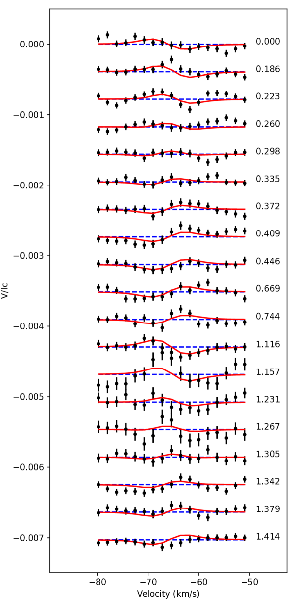
Figure 6: Stokes $V$ LSD profiles obtained with Neo-NARVAL (black dots), and synthetic profiles produced by ZDI (red curves). Successive observations are vertically shifted for clarity, and the rotational phase $\Phi$ of the observation is listed along the right side.

Running ZDI (Semel, 1989) on polarization signatures close to the detection threshold is not ideal, but previous studies have shown that it is possible to reconstruct magnetic maps even when the signatures are dominated by noise, provided that a sufficient number of observations are combined together in the inversion process (Petit et al., 2010, 2022). Here, we use the ZDI implementation of Folsom et al. (2018a, b), in a procedure closely following the one presented by Petit et al. (2021). The surface magnetic field is described by the set of spherical harmonic equations in Donati et al. (2006), and we limited the expansion to $\ell_{\rm max}=10$ because the magnetic model was not improved by including higher-order terms.

We adopted a projected rotational velocity of 2 km s^-1 (Brewer et al., 2016), resulting in an inclination angle of 50^∘ when combined with our estimates of $P_{\rm rot}$ and $R$. The radial velocity of our LSD profiles was $-$65.9 km s^-1, which is about 0.5 km s^-1 larger than recent estimates (Soubiran et al., 2018). Following Petit et al. (2008), we ran a series of ZDI inversions assuming different values of the rotation period and found that the best fit was obtained for $P_{\rm rot}=26.87$ d. Following this estimate, the rotational phase $\Phi$ of each observation was calculated using the following ephemeris:

$$\mathit{HJD}_{\mathrm{obs}}=\mathit{HJD}_{0}+P_{\rm{rot}}\times\Phi$$ (8)

where the initial Heliocentric Julian date $\mathit{HJD}_{0}$ was from our first observation at 2459406.373. It is clear from Figure 6 that the phase coverage is very good between $\Phi=0$ and 0.4 (observed over two consecutive rotation cycles), while only two observations have phases above 0.5. We also performed a search for differential rotation following the method of Petit et al. (2002) but failed to measure a surface shear. The target reduced $\chi^{2}$ of the ZDI inversion was fixed at 1.075, because adopting lower values led to clear signs of overfitting (visible as a sharp increase in the average field strength and field complexity). The resulting map is shown in Figure 7, while the synthetic Stokes $V$ LSD profiles are plotted with red lines in Figure 6.

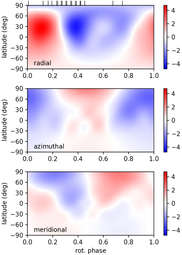
Figure 7: Large-scale surface magnetic geometry of $\lambda$ Ser. The three panels display the field components in spherical coordinates, adopting an equatorial projection. Color bars on the right show the field strength in Gauss. Vertical ticks above the top panel indicate observed rotational phases. Latitudes below $-40^{\circ}$ are not observed.

The reconstructed magnetic geometry has an average field strength of 2 G, with a maximum local peak strength of 5 G. A majority of the magnetic energy (87%) shows up in the poloidal field component, and more specifically in the dipole component that hosts 71% of the poloidal magnetic energy. The dipole strength is equal to 2.9 G, and it is very inclined with respect to the spin axis, with a negative pole located at latitude $\sim$11^∘. Unsurprisingly, this very non-axisymmetric magnetic configuration leads to only 9% of the magnetic energy in modes with $m=0$.

Considering the low amplitude of polarization signatures in the Neo-NARVAL LSD profiles, we carried out an independent ZDI reconstruction with an alternative inversion code (Kochukhov et al., 2014; Rosén et al., 2016; Lehtinen et al., 2022). This inversion adopted the same $P_{\rm rot}$, $\ell_{\rm max}$, $i$, and $v_{\rm e}\sin i$, resulting in a qualitatively similar magnetic field distribution to the one illustrated in Figure 7 but with a somewhat stronger and more structured magnetic field map. In this case, we found an average field strength of 3.7 G and a maximum local strength of 8.9 G. Contributions of the poloidal and toroidal components are nearly equal, with the dipole component containing 48% of the total magnetic field energy and 31% of the poloidal field energy. The discrepancies of these parameters with the outcome of the first ZDI reconstruction likely reflect intrinsic limitations of ZDI based on low S/N data. Nevertheless, the dipole field characteristics (strength 2.1 G, obliquity 98° towards the positive pole) are similar to those obtained in the first inversion.

To estimate the rate of angular momentum loss for $\lambda$ Ser, we use the braking law of Finley & Matt (2018) (see Section 3.4). This braking law requires the polar strengths of the dipole, quadrupole and octupole components of stellar magnetic field as inputs. These can be obtained from the reconstructed ZDI maps. However, the magnetohydrodynamic simulations used to construct the Finley & Matt (2018) braking law were run using only axisymmetric magnetic field modes whereas the ZDI maps contain both axisymmetric and non-axisymmetric components. In order to calculate the equivalent polar field strengths needed for the braking law from each ZDI map, we used the method we employed in Metcalfe et al. (2022). Briefly, this method calculates the magnetic flux in each of the dipole, quadrupole and octupole components of the ZDI map, i.e. accounting for both the axisymmetric and non-axisymmetric components. We then determine the polar field strengths of a purely axisymmetric dipole, quadrupole and octupole that reproduces the respective magnetic fluxes of each component from the ZDI map. These are the field strengths reported in Table 3.1 (first, second reconstruction) and used in the braking law.

3.3 Rotational Evolution

We fit a rotational evolution model to $\lambda$ Ser following the methodology described in Metcalfe et al. (2020). We use slightly different values for two braking law parameters: a braking normalization of $f_{k}=8.53$ for the standard law and $f_{k}=8.97$ and Ro${}_{\rm crit}=2.01$ for the weakened magnetic braking law, derived from calibrating the braking law to the asteroseismic rotator sample of Hall et al. (2021), open clusters, and the Sun (Saunders et al. in prep). This amounts to a braking normalization that is $\sim$40% higher and Ro_crit that is 7% lower than that used in Metcalfe et al. (2020) for the weakened law, and a braking normalization $\sim$25% higher for the standard law. These changes would tend to make a star of a given age and mass spin more slowly, although weakened magnetic braking occurs at slightly faster rotation rates.

We search for a best-fit model that matches our observed surface temperature, luminosity, and surface metallicity, with asteroseismic priors on the mass, age, and mixing length as described in Metcalfe et al. (2020). Our best-fit model reproduces all surface observables and priors (with the exception of rotation) within $1\sigma$. For a standard model, we predict a rotation period of $34\pm 6$ days, while weakened magnetic braking predicts a period of $18\pm 2$ days. The weakened magnetic braking model is consistent with the most rapid seasonal rotation rate observed for $\lambda$ Ser. If $\lambda$ Ser is in fact viewed at a moderate inclination and has solar-like differential rotation, we might expect the observed rotation period to be slower than the equatorial rotation period that is predicted by the solid body stellar models. However, its mean rotation period is in mild tension with both the weakened magnetic braking and standard case, and does not conclusively distinguish between the two scenarios.

3.4 Magnetic Evolution

Bringing together the magnetic field properties derived in Section 3.2, the mass-loss rate estimated in Section 2.3, the range of rotation periods measured in Section 2.4, and the asteroseismic radius and mass from Section 3.1, we can use the prescription of Finley & Matt (2018) to estimate the wind braking torque of $\lambda$ Ser. We repeat the calculation using the magnetic field properties ($B_{d},B_{q},B_{o}$) from two independent ZDI reconstructions that relied on the same set of Stokes $V$ profiles (see Section 3.2). In Table 3.1 we report the average torque resulting from the two calculations, and we adopt half of the difference between them as the uncertainty arising from the magnetic field properties (11%). The total uncertainty on the torque includes additional contributions from the rotation period (6%), mass-loss rate (4%), radius (4%), and mass (1%), and it reflects the range of possible torques when all quantities are shifted by $\pm 1\sigma$.

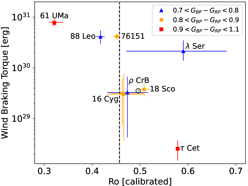
Figure 8: Evolution of the wind braking torque with Ro from the calibration of Corsaro et al. (2021). Points are grouped by Gaia color, corresponding to solar analogs (yellow circles), and hotter (blue triangles) or cooler stars (red squares). The empirical constraint for Ro_crit on this scale is shown with a vertical dashed line.

The estimated wind braking torque for $\lambda$ Ser is shown relative to several other stars in Figure 8. We calculate the Rossby number for each star from the Gaia $G_{BP}-G_{RP}$ color, using the asteroseismic calibration from Corsaro et al. (2021). We estimate the wind braking torque following the methodology outlined in Metcalfe et al. (2021, 2022), while the solar point ($\odot$) comes from Finley et al. (2018). On this scale, the empirical value of the Rossby number that corresponds to the onset of weakened magnetic braking is ${\rm Ro_{crit}}=0.46$ (dashed line). The horizontal error bar for $\lambda$ Ser corresponds to the range of seasonal rotation periods identified in Section 2.4, while the vertical error bar is dominated by uncertainties in the strength and morphology of the large-scale magnetic field (see Section 3.2), with progressively smaller contributions from the rotation period, mass-loss rate, radius, and mass. Even considering the uncertainties, the wind braking torque for $\lambda$ Ser is much higher than for other stars with similar Ro (cf. $\tau$ Cet; Metcalfe et al., 2023).

The relatively high wind braking torque for $\lambda$ Ser cannot easily be attributed to an erroneous measurement. Our previous LBT observations of flat activity stars ($\rho$ CrB, 16 Cyg A & B) resulted in null detections, while the Stokes $V$ signature for $\lambda$ Ser is strong and consistent with the lower S/N measurements from TBL. There is considerable scatter in the Wood et al. (2021) relation between X-ray flux and mass-loss rate, but the two subgiants in the calibration both have higher mass-loss rates than predicted from their X-ray flux. Despite the low mean activity level, the rotation rate inferred from MWO observations appears consistently in multiple seasons and across the complete data set. The radius and mass inferred from asteroseismology are both precise, and they agree with the independent estimates from the SED in Section 2.5. The difficulty of matching the stellar properties with rotational evolution models that assume either standard spin-down or weakened magnetic braking also suggests that $\lambda$ Ser may have taken an unusual path to its present configuration. The asteroseismic age is consistent with the activity-age relation for solar analogs (Huber et al., 2022), but the remaining uncertainty prevents an unambiguous interpretation of the other stellar properties.

4 Discussion

Our data on $\lambda$ Ser adds an interesting piece to our understanding of rotation, magnetism, and dynamos in old sun-like stars. Stars more active than the Sun spin down as they age, so it is natural to extrapolate this behavior to older and less active stars. However, it is not surprising that our intuition, developed in a limited empirical domain, would break down in the face of the time domain revolution in stellar astrophysics. The first hint was the lack of very slowly rotating stars in the groundbreaking McQuillan et al. (2014) Kepler sample. The Sun, a median-aged disk star, was at the upper end of the observed distribution of stellar rotation periods on the main sequence. However, this could be induced either by a true cessation of spin-down or a threshold in detectability (van Saders et al., 2019). A much stronger indication of disrupted magnetic braking was the discovery of counter-examples: stars rotating too rapidly to have experienced the degree of magnetic braking predicted by standard models. The observed pattern favored a dramatic decrease in the efficacy of magnetized winds above a critical Rossby threshold (van Saders et al., 2016). This phenomenon requires a transition such that inactive stars experience minimal angular momentum losses over long timescales. It does not directly test the origin of this transition, or the degree to which it is sudden rather than gradual.

In a series of papers (Metcalfe et al., 2021, 2022, 2023) we have mapped out the magnetic field strength and morphology of stars close to the disrupted magnetic braking threshold, and used these data to infer integrated instantaneous angular momentum loss rates. We have found striking evidence of a dichotomy between stars with “normal” field strengths and derived torques and those with low field strengths and small derived torques. Prior to $\lambda$ Ser, these categories corresponded well to expectations for a disrupted magnetic braking model. At first glance, $\lambda$ Ser appears to be an exception: it is in the “normal” field and torque state, but has a Rossby number beyond that predicted by a simple cutoff model. This intriguing result has a number of potential causes—we will begin with those consistent with the disrupted braking hypothesis.

The simplest explanation is a mechanical error in the derived stellar properties. For example, if the overturn timescale were longer or if we adopted a different age, $\lambda$ Ser might line up with expectations. Although this is certainly possible, we consider it unlikely based on our error model. A second variant would be that $\lambda$ Ser has experienced an unusual angular momentum history—for example, either a stellar merger or engulfment of a large planet. These events are actually not unusual for low mass stars, and they would reset the rotation and activity “clock” such that more rapid rotation and higher activity could be expected. Andronov et al. (2006) estimated that of order 4% of stars in this mass and age range are actually merger products. However, field merger products tend to be Li-poor (Ryan et al., 2002), while $\lambda$ Ser is Li-rich (Xing & Xing, 2012). A stellar-mass merger is thus disfavored, but late engulfment of a giant planet could account for the Li abundance and induce significant spin-up, particularly as stars age and begin to leave the main sequence. Exact rates are uncertain, but this cannot be ruled out at the few percent level (Ahuir et al., 2021). If apparent counter-examples like $\lambda$ Ser are rare, these explanations—errors in stellar measurements or an unusual history—would become more plausible.

A different family of solutions focuses instead on the nature of the threshold transition. Although a Rossby formulation is widely used in activity studies, it may be inadequate to capture the full picture. We are using evolutionary models of evolved stars, while traditional Rossby studies are confined to unevolved near-MS stars. As a result, traditional “Rossby” scaling can also be viewed as expressing a dependence of stellar activity on, say, effective temperature. The alignment with theoretical overturn timescales could be a happy coincidence. It may therefore be helpful to revisit the question of whether Rossby number really does serve as a valid dynamo diagnostic in the evolved and low activity domain. A variant of this hypothesis would be a duty cycle argument—in such a model, the transition from low to high state is not abrupt, but instead gradual. An example in the history of the Sun would be the existence of a Maunder minimum phase. In the transition domain between the active and inactive branches, stars would cycle between active and inactive phases over an extended period of time (Vashishth et al., 2023). Such a pattern could be revealed with a larger sample of stars, sufficient to infer statistically significant samples for hypothesis testing.

The evolutionary status of $\lambda$ Ser is ambiguous, at least in part, due to a weak constraint on the stellar age from asteroseismology. The age can be constrained from the frequency difference between radial ($l=0$) oscillation modes that sample the composition in the stellar core and neighboring quadrupole ($l=2$) modes that do not pass through this region. The non-detection of $l=2$ modes in $\lambda$ Ser is unusual for stars in this temperature range (Lund et al., 2017), and prevents a determination of the small frequency separation ($\delta\nu_{02}$) that would otherwise provide a stronger constraint on the stellar age. Unfortunately, additional TESS observations of $\lambda$ Ser will not be available until 2026 at the earliest, because the position of Sector 78 was shifted northward to avoid scattered light from the Earth and Moon. However, ground-based radial velocity observations are less impacted by the background noise from stellar granulation (García & Ballot, 2019), yielding a higher S/N than photometry and improving the potential to detect low-amplitude oscillation modes. Future observations of $\lambda$ Ser by the Stellar Observations Network Group (SONG; Grundahl et al., 2008) may provide a measurement of $\delta\nu_{02}$ that could substantially improve the age precision and help resolve this ambiguity.

This paper includes data collected with the TESS mission, obtained from the Mikulski Archive for Space Telescopes (MAST) at the Space Telescope Science Institute (STScI). The specific observations analyzed can be accessed via https://doi.org/10.17909/ar5x-2g05 (catalog doi:10.17909/ar5x-2g05). Funding for the TESS mission is provided by the NASA Explorer Program. STScI is operated by the Association of Universities for Research in Astronomy, Inc., under NASA contract NAS 5–26555. T.S.M. acknowledges support from Chandra award GO0-21005X, NASA grant 80NSSC22K0475, NSF grant AST-2205919, and the Vanderbilt Initiative in Data-intensive Astrophysics (VIDA). Computational time at the Texas Advanced Computing Center was provided through XSEDE allocation TG-AST090107. D.B. gratefully acknowledges support from NASA (NNX16AB76G, 80NSSC22K0622) and the Whitaker Endowed Fund at Florida Gulf Coast University. D.H. acknowledges support from the Alfred P. Sloan Foundation, NASA (80NSSC22K0303, 80NSSC23K0434, 80NSSC23K0435), and the Australian Research Council (FT200100871). J.v.S acknowledges support from NSF grant AST-2205919. S.B. acknowledges NSF grant AST-2205026. O.K. acknowledges support by the Swedish Research Council (grant agreement no. 2019-03548), the Swedish National Space Agency, and the Royal Swedish Academy of Sciences. S.H.S. is grateful for support from award HST-GO-15991.002-A. V.S. acknowledges support from the European Space Agency (ESA) as an ESA Research Fellow. T.R.B. acknowledges support from the Australian Research Council (Laureate Fellowship FL220100117). S.N.B. acknowledges support from PLATO ASI-INAF agreement n. 2015-019-R.1-2018. A.J.F. acknowledges support from the European Research Council (ERC) under the European Union’s Horizon 2020 research and innovation programme (grant agreement No 810218 WHOLESUN). R.A.G. acknowledges support from the PLATO and GOLF Centre National D’Études Spatiales (CNES) grant. Funding for the Stellar Astrophysics Centre is provided by The Danish National Research Foundation (Grant agreement No. DNRF106). M.B.N. acknowledges support from the UK Space Agency. A.S. acknowledges support from the European Research Council Consolidator Grant funding scheme (project ASTEROCHRONOMETRY, G.A. n. 772293, http://www.asterochronometry.eu). C.A.C. acknowledges that this research was carried out at the Jet Propulsion Laboratory, California Institute of Technology, under a contract with NASA (80NM0018D0004). D.G.R. acknowledges support from the Spanish Ministry of Science and Innovation (MICINN) grant no. PID2019-107187GB-I00. K.G.S. thanks the German Federal Ministry (BMBF) for the year-long support for the construction of PEPSI through their Verbundforschung grants 05AL2BA1/3 and 05A08BAC as well as the State of Brandenburg for the continuing support of the LBT (see https://pepsi.aip.de/). LBT Corporation partners are the University of Arizona on behalf of the Arizona university system; Istituto Nazionale di Astrofisica, Italy; LBT Beteiligungsgesellschaft, Germany, representing the Max-Planck Society, the Leibniz-Institute for Astrophysics Potsdam (AIP), and Heidelberg University; the Ohio State University; and the Research Corporation, on behalf of the University of Notre Dame, University of Minnesota and University of Virginia. S.V.J. acknowledges the support of the DFG priority program SPP 1992 “Exploring the Diversity of Extrasolar Planets” (JE 701/5-1). A.A.V. acknowledges funding from the European Research Council (ERC) under the European Union’s Horizon 2020 research and innovation programme (grant agreement No 817540, ASTROFLOW).

Appendix A Asteroseismic Non-detections from TESS

Using the same procedure outlined in Section 2.1, we produced light curves for targets that both had 20 s cadence data and fell along the evolutionary sequences for our spectropolarimetric targets (Table 6). For these eight targets, we were able to improve on the quality of the light curve from the SPOC product. The light curves were analyzed for oscillations using pySYD (Chontos et al., 2022; Huber et al., 2009), yielding a null detection in all cases.

To derive upper limits, we evaluated the fitted background model from pySYD at the predicted $\nu_{\textrm{max}}$ value for each target and required a height-to-background ratio of 1.1 (Mosser et al., 2012), which is typically sufficient for a detection of oscillations. The corresponding amplitude limits are listed in Table 6 and compared to Kepler detections from Huber et al. (2011) in Figure 9. To account for differences in the TESS and Kepler bandpass, we reduced the amplitude limits by a factor 0.8 (Campante et al., 2016). The derived limits are consistent with null-detections for all stars. For the two stars with the lowest predicted $\nu_{\textrm{max}}$ ($\iota$ Hor and 88 Leo) the limits are below some Kepler detections, implying that their amplitudes may be suppressed by stellar magnetic activity (García et al., 2010; Chaplin et al., 2011; Mathur et al., 2019).

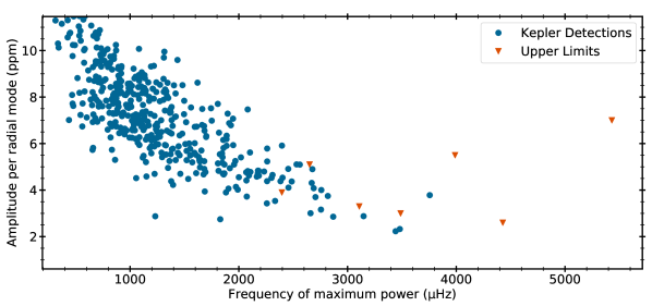
Figure 9: Amplitude per radial mode for stars observed by Kepler (blue circles; Huber et al., 2011) compared to the upper amplitude limits derived from TESS for stars with 20 s cadence data that fall along evolutionary sequences for our spectropolarimetric targets (orange triangles). Note that the upper limit for $\epsilon$ Eri is off-scale at 30.5, far above the markers in the legend.

Table 6: Upper limits on the detection of solar-like oscillations with TESS

Target	HD	Sector(s)	$T_{\rm eff}$	$\log g$	[M/H]	$\nu_{\rm max}$ ($\mu$Hz)	$A_{\rm lim}$ (ppm)
$\iota$ Hor	17051	30	6097	4.34	+0.09	2396	3.9
$\kappa^{1}$ Cet	20630	31	5742	4.49	+0.10	3488	3.0
$\epsilon$ Eri	22049	31	5146	4.57	+0.00	4430	30.5
40 Eri	26965	32	5151	4.57	$-$0.08	4428	2.6
HD 76151	76151	34	5790	4.55	+0.07	3989	5.5
88 Leo	100180	45, 49	5989	4.38	$-$0.02	2651	5.1
61 UMa	101501	49	5488	4.43	$-$0.03	3108	3.3
HD 103095	103095	49	4950	4.65	$-$1.16	5431	7.0

References

- Adelberger et al. (1998) Adelberger, E. G., Austin, S. M., Bahcall, J. N., et al. 1998, Reviews of Modern Physics, 70, 1265, doi: 10.1103/RevModPhys.70.1265
- Aguirre Børsen-Koch et al. (2022) Aguirre Børsen-Koch, V., Rørsted, J. L., Justesen, A. B., et al. 2022, MNRAS, 509, 4344, doi: 10.1093/mnras/stab2911
- Ahuir et al. (2021) Ahuir, J., Strugarek, A., Brun, A. S., & Mathis, S. 2021, A&A, 650, A126, doi: 10.1051/0004-6361/202040173
- Andronov et al. (2006) Andronov, N., Pinsonneault, M. H., & Terndrup, D. M. 2006, ApJ, 646, 1160, doi: 10.1086/505127
- Antia & Basu (1994) Antia, H. M., & Basu, S. 1994, A&AS, 107, 421
- Appourchaux et al. (2012) Appourchaux, T., Benomar, O., Gruberbauer, M., et al. 2012, A&A, 537, A134, doi: 10.1051/0004-6361/201118496
- Aurière (2003) Aurière, M. 2003, in EAS Publications Series, Vol. 9, EAS Publications Series, ed. J. Arnaud & N. Meunier, 105
- Ayres & Buzasi (2022) Ayres, T., & Buzasi, D. 2022, ApJS, 263, 41, doi: 10.3847/1538-4365/ac8cfc
- Ayres (2020) Ayres, T. R. 2020, ApJS, 250, 16, doi: 10.3847/1538-4365/aba3c6
- Baliunas et al. (1996) Baliunas, S., Sokoloff, D., & Soon, W. 1996, ApJ, 457, L99, doi: 10.1086/309891
- Baliunas et al. (1983) Baliunas, S. L., Hartmann, L., Noyes, R. W., et al. 1983, ApJ, 275, 752, doi: 10.1086/161572
- Baliunas et al. (1995) Baliunas, S. L., Donahue, R. A., Soon, W. H., et al. 1995, ApJ, 438, 269, doi: 10.1086/175072
- Ball & Gizon (2014) Ball, W. H., & Gizon, L. 2014, A&A, 568, A123, doi: 10.1051/0004-6361/201424325
- Baum et al. (2022) Baum, A. C., Wright, J. T., Luhn, J. K., & Isaacson, H. 2022, AJ, 163, 183, doi: 10.3847/1538-3881/ac5683
- Bedding et al. (2007) Bedding, T. R., Kjeldsen, H., Arentoft, T., et al. 2007, ApJ, 663, 1315, doi: 10.1086/518593
- Borucki et al. (2010) Borucki, W. J., Koch, D., Basri, G., et al. 2010, Science, 327, 977, doi: 10.1126/science.1185402
- Brage et al. (1996) Brage, T., Judge, P. G., & Brekke, P. 1996, ApJ, 464, 1030, doi: 10.1086/177390
- Breton et al. (2022) Breton, S. N., García, R. A., Ballot, J., Delsanti, V., & Salabert, D. 2022, A&A, 663, A118, doi: 10.1051/0004-6361/202243330
- Brewer et al. (2016) Brewer, J. M., Fischer, D. A., Valenti, J. A., & Piskunov, N. 2016, ApJS, 225, 32, doi: 10.3847/0067-0049/225/2/32
- Buzasi et al. (2015) Buzasi, D. L., Carboneau, L., Hessler, C., Lezcano, A., & Preston, H. 2015, in IAU General Assembly, Vol. 29, 2256843
- Campante et al. (2016) Campante, T. L., Schofield, M., Kuszlewicz, J. S., et al. 2016, ApJ, 830, 138, doi: 10.3847/0004-637X/830/2/138
- Carlos et al. (2016) Carlos, M., Nissen, P. E., & Meléndez, J. 2016, A&A, 587, A100, doi: 10.1051/0004-6361/201527478
- Chaplin et al. (2011) Chaplin, W. J., Bedding, T. R., Bonanno, A., et al. 2011, ApJ, 732, L5, doi: 10.1088/2041-8205/732/1/L5
- Chontos et al. (2022) Chontos, A., Huber, D., Sayeed, M., & Yamsiri, P. 2022, The Journal of Open Source Software, 7, 3331, doi: 10.21105/joss.03331
- Christensen-Dalsgaard (2008) Christensen-Dalsgaard, J. 2008, Ap&SS, 316, 13, doi: 10.1007/s10509-007-9675-5
- Corsaro et al. (2021) Corsaro, E., Bonanno, A., Mathur, S., et al. 2021, A&A, 652, L2, doi: 10.1051/0004-6361/202141395
- Corsaro & De Ridder (2014) Corsaro, E., & De Ridder, J. 2014, A&A, 571, A71, doi: 10.1051/0004-6361/201424181
- Corsaro et al. (2015) Corsaro, E., De Ridder, J., & García, R. A. 2015, A&A, 579, A83, doi: 10.1051/0004-6361/201525895
- Demarque et al. (2008) Demarque, P., Guenther, D. B., Li, L. H., Mazumdar, A., & Straka, C. W. 2008, Ap&SS, 316, 31, doi: 10.1007/s10509-007-9698-y
- Donahue (1993) Donahue, R. A. 1993, PhD thesis, New Mexico State University
- Donahue et al. (1996) Donahue, R. A., Saar, S. H., & Baliunas, S. L. 1996, ApJ, 466, 384, doi: 10.1086/177517
- Donati et al. (1997) Donati, J.-F., Semel, M., Carter, B. D., Rees, D. E., & Collier Cameron, A. 1997, MNRAS, 291, 658
- Donati et al. (1992) Donati, J. F., Semel, M., & Rees, D. E. 1992, A&A, 265, 669
- Donati et al. (2006) Donati, J.-F., Howarth, I. D., Jardine, M. M., et al. 2006, MNRAS, 370, 629, doi: 10.1111/j.1365-2966.2006.10558.x
- Egeland (2017) Egeland, R. 2017, PhD thesis, Montana State University, Bozeman, Montana, USA
- Egeland et al. (2017) Egeland, R., Soon, W., Baliunas, S., et al. 2017, ApJ, 835, doi: 10.3847/1538-4357/835/1/25
- Ferguson et al. (2005) Ferguson, J. W., Alexander, D. R., Allard, F., et al. 2005, ApJ, 623, 585, doi: 10.1086/428642
- Finley & Matt (2018) Finley, A. J., & Matt, S. P. 2018, ApJ, 854, 78, doi: 10.3847/1538-4357/aaaab5
- Finley et al. (2018) Finley, A. J., Matt, S. P., & See, V. 2018, ApJ, 864, 125, doi: 10.3847/1538-4357/aad7b6
- Folsom et al. (2018a) Folsom, C. P., Bouvier, J., Petit, P., et al. 2018a, MNRAS, 474, 4956, doi: 10.1093/mnras/stx3021
- Folsom et al. (2018b) Folsom, C. P., Fossati, L., Wood, B. E., et al. 2018b, MNRAS, 481, 5286, doi: 10.1093/mnras/sty2494
- Formicola et al. (2004) Formicola, A., Imbriani, G., Costantini, H., et al. 2004, Physics Letters B, 591, 61, doi: 10.1016/j.physletb.2004.03.092
- Fruscione et al. (2006) Fruscione, A., McDowell, J. C., Allen, G. E., et al. 2006, in Society of Photo-Optical Instrumentation Engineers (SPIE) Conference Series, Vol. 6270, Society of Photo-Optical Instrumentation Engineers (SPIE) Conference Series, ed. D. R. Silva & R. E. Doxsey, 62701V
- Gai et al. (2011) Gai, N., Basu, S., Chaplin, W. J., & Elsworth, Y. 2011, ApJ, 730, 63, doi: 10.1088/0004-637X/730/2/63
- García & Ballot (2019) García, R. A., & Ballot, J. 2019, Living Reviews in Solar Physics, 16, 4, doi: 10.1007/s41116-019-0020-1
- García et al. (2010) García, R. A., Mathur, S., Salabert, D., et al. 2010, Science, 329, 1032, doi: 10.1126/science.1191064
- García et al. (2009) García, R. A., Régulo, C., Samadi, R., et al. 2009, A&A, 506, 41, doi: 10.1051/0004-6361/200911910
- García et al. (2011) García, R. A., Hekker, S., Stello, D., et al. 2011, MNRAS, 414, L6, doi: 10.1111/j.1745-3933.2011.01042.x
- Gregory & Loredo (1992) Gregory, P. C., & Loredo, T. J. 1992, ApJ, 398, 146, doi: 10.1086/171844
- Grundahl et al. (2008) Grundahl, F., Christensen–Dalsgaard, J., Arentoft, T., et al. 2008, Communications in Asteroseismology, 157, 273
- Hall et al. (2007) Hall, J. C., Lockwood, G. W., & Skiff, B. A. 2007, AJ, 133, 862, doi: 10.1086/510356
- Hall et al. (2021) Hall, O. J., Davies, G. R., van Saders, J., et al. 2021, Nature Astronomy, 5, 707, doi: 10.1038/s41550-021-01335-x
- Handberg & Campante (2011) Handberg, R., & Campante, T. L. 2011, A&A, 527, A56, doi: 10.1051/0004-6361/201015451
- Horne & Baliunas (1986) Horne, J. H., & Baliunas, S. L. 1986, ApJ, 302, 757, doi: 10.1086/164037
- Huber et al. (2009) Huber, D., Stello, D., Bedding, T. R., et al. 2009, Communications in Asteroseismology, 160, 74, doi: 10.48550/arXiv.0910.2764
- Huber et al. (2011) Huber, D., Bedding, T. R., Arentoft, T., et al. 2011, ApJ, 731, 94, doi: 10.1088/0004-637X/731/2/94
- Huber et al. (2022) Huber, D., White, T. R., Metcalfe, T. S., et al. 2022, AJ, 163, 79, doi: 10.3847/1538-3881/ac3000
- Iglesias & Rogers (1996) Iglesias, C. A., & Rogers, F. J. 1996, ApJ, 464, 943, doi: 10.1086/177381
- Isaacson & Fischer (2010) Isaacson, H., & Fischer, D. 2010, ApJ, 725, 875, doi: 10.1088/0004-637X/725/1/875
- Joyce & Chaboyer (2018) Joyce, M., & Chaboyer, B. 2018, ApJ, 864, 99, doi: 10.3847/1538-4357/aad464
- Judge (2020) Judge, P. G. 2020, MNRAS, 491, 576, doi: 10.1093/mnras/stz3063
- Keenan et al. (1988) Keenan, F. P., Dufton, P. L., Aggarwal, K. M., & Kingston, A. E. 1988, ApJ, 324, 1068, doi: 10.1086/165963
- Keenan et al. (1990) Keenan, F. P., Dufton, P. L., & Kingston, A. E. 1990, ApJ, 353, 636, doi: 10.1086/168653
- Keenan et al. (1987) Keenan, F. P., Kingston, A. E., & Dufton, P. L. 1987, MNRAS, 225, 859, doi: 10.1093/mnras/225.4.859
- Kjeldsen et al. (2005) Kjeldsen, H., Bedding, T. R., Butler, R. P., et al. 2005, ApJ, 635, 1281, doi: 10.1086/497530
- Kochukhov (2016) Kochukhov, O. 2016, in Lecture Notes in Physics, Berlin Springer Verlag, ed. J.-P. Rozelot & C. Neiner, Vol. 914 (Springer, Berlin), 177
- Kochukhov et al. (2014) Kochukhov, O., Lüftinger, T., Neiner, C., Alecian, E., & MiMeS Collaboration. 2014, A&A, 565, A83, doi: 10.1051/0004-6361/201423472
- Kochukhov et al. (2010) Kochukhov, O., Makaganiuk, V., & Piskunov, N. 2010, A&A, 524, A5, doi: 10.1051/0004-6361/201015429
- Landi Degl’Innocenti (1992) Landi Degl’Innocenti, E. 1992, Magnetic field measurements. (Cambridge University Press, Cambridge), 71
- Lehtinen et al. (2022) Lehtinen, J. J., Käpylä, M. J., Hackman, T., et al. 2022, A&A, 660, A141, doi: 10.1051/0004-6361/201936780
- Lenz & Breger (2005) Lenz, P., & Breger, M. 2005, Communications in Asteroseismology, 146, 53, doi: 10.1553/cia146s53
- Li et al. (2020) Li, Y., Bedding, T. R., Li, T., et al. 2020, MNRAS, 495, 2363, doi: 10.1093/mnras/staa1335
- Li et al. (2023) Li, Y., Bedding, T. R., Stello, D., et al. 2023, MNRAS, 523, 916, doi: 10.1093/mnras/stad1445
- Lomb (1976) Lomb, N. R. 1976, Ap&SS, 39, 447, doi: 10.1007/BF00648343
- López Ariste et al. (2022) López Ariste, A., Georgiev, S., Mathias, P., et al. 2022, A&A, 661, A91, doi: 10.1051/0004-6361/202142271
- Lund et al. (2017) Lund, M. N., Silva Aguirre, V., Davies, G. R., et al. 2017, ApJ, 835, 172, doi: 10.3847/1538-4357/835/2/172
- Marsden et al. (2014) Marsden, S. C., Petit, P., Jeffers, S. V., et al. 2014, MNRAS, 444, 3517, doi: 10.1093/mnras/stu1663
- Mathis & Neiner (2015) Mathis, S., & Neiner, C. 2015, in New Windows on Massive Stars, ed. G. Meynet, C. Georgy, J. Groh, & P. Stee, Vol. 307, 420–425
- Mathur et al. (2019) Mathur, S., García, R. A., Bugnet, L., et al. 2019, Frontiers in Astronomy and Space Sciences, 6, 46, doi: 10.3389/fspas.2019.00046
- McQuillan et al. (2014) McQuillan, A., Mazeh, T., & Aigrain, S. 2014, ApJS, 211, 24, doi: 10.1088/0067-0049/211/2/24
- Mermilliod (2006) Mermilliod, J. C. 2006, VizieR Online Data Catalog, II/168
- Metcalfe et al. (2009) Metcalfe, T. S., Creevey, O. L., & Christensen-Dalsgaard, J. 2009, ApJ, 699, 373, doi: 10.1088/0004-637X/699/1/373
- Metcalfe et al. (2019) Metcalfe, T. S., Kochukhov, O., Ilyin, I. V., et al. 2019, ApJ, 887, L38, doi: 10.3847/2041-8213/ab5e48
- Metcalfe et al. (2020) Metcalfe, T. S., van Saders, J. L., Basu, S., et al. 2020, ApJ, 900, 154, doi: 10.3847/1538-4357/aba963
- Metcalfe et al. (2021) —. 2021, ApJ, 921, 122, doi: 10.3847/1538-4357/ac1f19
- Metcalfe et al. (2022) Metcalfe, T. S., Finley, A. J., Kochukhov, O., et al. 2022, ApJ, 933, L17, doi: 10.3847/2041-8213/ac794d
- Metcalfe et al. (2023) Metcalfe, T. S., Strassmeier, K. G., Ilyin, I. V., et al. 2023, ApJ, 948, L6, doi: 10.3847/2041-8213/acce38
- Morel (2018) Morel, T. 2018, A&A, 615, A172, doi: 10.1051/0004-6361/201833125
- Mosser et al. (2012) Mosser, B., Elsworth, Y., Hekker, S., et al. 2012, A&A, 537, A30, doi: 10.1051/0004-6361/201117352
- Nason (2006) Nason, G. 2006, Stationary and non-stationary time series (United Kingdom: Geological Society of London), 129 – 142
- Nielsen et al. (2020) Nielsen, M. B., Ball, W. H., Standing, M. R., et al. 2020, A&A, 641, A25, doi: 10.1051/0004-6361/202037461
- Paunzen (2015) Paunzen, E. 2015, A&A, 580, A23, doi: 10.1051/0004-6361/201526413
- Paxton et al. (2015) Paxton, B., Marchant, P., Schwab, J., et al. 2015, ApJS, 220, 15, doi: 10.1088/0067-0049/220/1/15
- Petit et al. (2022) Petit, P., Böhm, T., Folsom, C. P., Lignières, F., & Cang, T. 2022, A&A, 666, A20, doi: 10.1051/0004-6361/202143000
- Petit et al. (2002) Petit, P., Donati, J.-F., & Collier Cameron, A. 2002, MNRAS, 334, 374, doi: 10.1046/j.1365-8711.2002.05529.x
- Petit et al. (2008) Petit, P., Dintrans, B., Solanki, S. K., et al. 2008, MNRAS, 388, 80, doi: 10.1111/j.1365-2966.2008.13411.x
- Petit et al. (2010) Petit, P., Lignières, F., Wade, G. A., et al. 2010, A&A, 523, A41, doi: 10.1051/0004-6361/201015307
- Petit et al. (2021) Petit, P., Folsom, C. P., Donati, J. F., et al. 2021, A&A, 648, A55, doi: 10.1051/0004-6361/202040027
- Prša et al. (2019) Prša, A., Zhang, M., & Wells, M. 2019, PASP, 131, 068001, doi: 10.1088/1538-3873/ab0f41
- Rao et al. (2022) Rao, Y. K., Del Zanna, G., Mason, H. E., & Dufresne, R. 2022, MNRAS, 517, 1422, doi: 10.1093/mnras/stac2772
- Ricker et al. (2014) Ricker, G. R., Winn, J. N., Vanderspek, R., et al. 2014, in Society of Photo-Optical Instrumentation Engineers (SPIE) Conference Series, Vol. 9143, Proceedings of the SPIE, Volume 9143, id. 914320 15 pp. (2014)., 914320
- Rogers & Nayfonov (2002) Rogers, F. J., & Nayfonov, A. 2002, ApJ, 576, 1064, doi: 10.1086/341894
- Rosén et al. (2016) Rosén, L., Kochukhov, O., Hackman, T., & Lehtinen, J. 2016, A&A, 593, A35, doi: 10.1051/0004-6361/201628443
- Rosenthal et al. (2021) Rosenthal, L. J., Fulton, B. J., Hirsch, L. A., et al. 2021, ApJS, 255, 8, doi: 10.3847/1538-4365/abe23c
- Ryabchikova et al. (2015) Ryabchikova, T., Piskunov, N., Kurucz, R. L., et al. 2015, Phys. Scr, 90, 054005, doi: 10.1088/0031-8949/90/5/054005
- Ryan et al. (2002) Ryan, S. G., Gregory, S. G., Kolb, U., Beers, T. C., & Kajino, T. 2002, ApJ, 571, 501, doi: 10.1086/339939
- Scargle (1982) Scargle, J. D. 1982, ApJ, 263, 835, doi: 10.1086/160554
- Semel (1989) Semel, M. 1989, A&A, 225, 456
- Semel et al. (1993) Semel, M., Donati, J. F., & Rees, D. E. 1993, A&A, 278, 231
- Soubiran et al. (2018) Soubiran, C., Jasniewicz, G., Chemin, L., et al. 2018, A&A, 616, A7, doi: 10.1051/0004-6361/201832795
- Stassun et al. (2017) Stassun, K. G., Collins, K. A., & Gaudi, B. S. 2017, AJ, 153, 136, doi: 10.3847/1538-3881/aa5df3
- Stassun et al. (2018) Stassun, K. G., Corsaro, E., Pepper, J. A., & Gaudi, B. S. 2018, AJ, 155, 22, doi: 10.3847/1538-3881/aa998a
- Stassun & Torres (2016) Stassun, K. G., & Torres, G. 2016, AJ, 152, 180, doi: 10.3847/0004-6256/152/6/180
- Stassun & Torres (2021) —. 2021, ApJ, 907, L33, doi: 10.3847/2041-8213/abdaad
- Strassmeier et al. (2015) Strassmeier, K. G., Ilyin, I., Järvinen, A., et al. 2015, Astronomische Nachrichten, 336, 324, doi: 10.1002/asna.201512172
- Thoul et al. (1994) Thoul, A. A., Bahcall, J. N., & Loeb, A. 1994, ApJ, 421, 828, doi: 10.1086/173695
- Torres et al. (2010) Torres, G., Andersen, J., & Giménez, A. 2010, A&A Rev., 18, 67, doi: 10.1007/s00159-009-0025-1
- van Saders et al. (2016) van Saders, J. L., Ceillier, T., Metcalfe, T. S., et al. 2016, Nature, 529, 181, doi: 10.1038/nature16168
- van Saders et al. (2019) van Saders, J. L., Pinsonneault, M. H., & Barbieri, M. 2019, ApJ, 872, 128, doi: 10.3847/1538-4357/aafafe
- Vanderburg & Johnson (2014) Vanderburg, A., & Johnson, J. A. 2014, PASP, 126, 948, doi: 10.1086/678764
- Vashishth et al. (2023) Vashishth, V., Karak, B. B., & Kitchatinov, L. 2023, MNRAS, 522, 2601, doi: 10.1093/mnras/stad1105
- Vaughan et al. (1978) Vaughan, A. H., Preston, G. W., & Wilson, O. C. 1978, PASP, 90, 267, doi: 10.1086/130324
- Viani & Basu (2017) Viani, L., & Basu, S. 2017, in European Physical Journal Web of Conferences, Vol. 160, European Physical Journal Web of Conferences, 05005
- Weiss et al. (2008) Weiss, W. W., Moffat, A. F. J., & Kudelka, O. 2008, Communications in Asteroseismology, 157, 271
- White & Livingston (1981) White, O. R., & Livingston, W. C. 1981, ApJ, 249, 798, doi: 10.1086/159338
- White et al. (2011) White, T. R., Bedding, T. R., Stello, D., et al. 2011, ApJ, 743, 161, doi: 10.1088/0004-637X/743/2/161
- Wilson (1978) Wilson, O. C. 1978, ApJ, 226, 379, doi: 10.1086/156618
- Wood et al. (2018) Wood, B. E., Laming, J. M., Warren, H. P., & Poppenhaeger, K. 2018, ApJ, 862, 66, doi: 10.3847/1538-4357/aaccf6
- Wood et al. (2021) Wood, B. E., Müller, H.-R., Redfield, S., et al. 2021, ApJ, 915, 37, doi: 10.3847/1538-4357/abfda5
- Xing & Xing (2012) Xing, L. F., & Xing, Q. F. 2012, A&A, 537, A91, doi: 10.1051/0004-6361/201117133