MS-XXXX

Network Interference Heterogeneity

A Two-Part Machine Learning Approach to Characterizing Network Interference in A/B Testing

Yuan Yuan Daniels School of Business, Purdue University, West Lafayette, IN, 47907, yuanyuan@purdue.edu Kristen M. Altenburger Central Applied Science, Meta Inc., Menlo Park, CA, 94025, kaltenburger@meta.com

The reliability of controlled experiments, or “A/B tests,” can often be compromised due to the phenomenon of network interference, wherein the outcome for one unit is influenced by other units. To tackle this challenge, we propose a machine learning-based method to identify and characterize heterogeneous network interference. Our approach accounts for latent complex network structures and automates the task of “exposure mapping” determination, which addresses the two major limitations in the existing literature. We introduce “causal network motifs” and employ transparent machine learning models to establish the most suitable exposure mapping that reflects underlying network interference patterns. Our method’s efficacy has been validated through simulations on two synthetic experiments and a real-world, large-scale test involving 1-2 million Instagram users, outperforming conventional methods such as design-based cluster randomization and analysis-based neighborhood exposure mapping. Overall, our approach not only offers a comprehensive, automated solution for managing network interference and improving the precision of A/B testing results, but it also sheds light on users’ mutual influence and aids in the refinement of marketing strategies.

experimental design, networks, interference, transparent machine learning, A/B testing

1 Introduction

Controlled experiments, also known as “A/B testing,” continue to serve as the cornerstone for making strategic decisions in business, including new product launches, marketing campaigns, and algorithm updates (Bakshy et al. 2014, Kohavi et al. 2020, Diamantopoulos et al. 2020, Bojinov and Gupta 2022, Koning et al. 2022). Through the random assignment of treatment or control groups, A/B testing facilitates the evaluation of causal, rather than merely correlational, impacts of a product intervention on business outcomes. Businesses have increasingly recognized the value of A/B testing and are investing in the development of in-house experimentation platforms (Tang et al. 2010, Kohavi et al. 2013, Bakshy et al. 2014, Xu et al. 2015). Furthermore, companies that have implemented A/B testing strategies have witnessed impressive performance improvements ranging from 30% to 100% after just one year of use (Koning et al. 2022).

However, a significant obstacle to the validity of A/B testing is network interference. Traditional causal inference rests on an essential assumption known as the “Stable Unit Treatment Value Assumption” (SUTVA) (Rubin 1980, 2005), which implies a unit’s outcome only depends on their treatment assignment. Network interference refers to a scenario where a unit’s (such as a person’s) outcome could also be influenced by the treatment assignments of other units, particularly those in their network neighborhood, if their connections are modeled as a network (Hudgens and Halloran 2008, Toulis and Kao 2013, Basse and Airoldi 2018). Here various types of networks may be involved, including social networks, location-based networks, or other networks developed based on shared attributes. Network interference is prevalent in numerous contemporary A/B testing environments, including social media, online marketplaces, and location-based platforms (Hagiu and Wright 2015, Yan et al. 2018, Holtz et al. 2020, Li et al. 2022). Failing to properly account for network interference is problematic. For instance, Holtz et al. (2020) found that network interference could skew the estimation of the treatment effect by more than 30%. Overall, network interference presents a significant challenge to industrial A/B tests, as it may mislead business decisions on product updates if the test’s results are unreliable.

Efforts to improve estimation in the presence of network interference have predominantly followed two research paths: pre-experimental design and post-experiment analysis (Eckles et al. 2016). The focus of experimental design is to devise improved randomization treatment assignments. A notable instance is graph cluster randomization (Ugander et al. 2013), a variant of cluster randomization (Bland 2004), which establishes graph clusters (communities) based on the graph structure and dispenses treatments at the level of these graph clusters. This field is extensive and has seen significant developments. Works such as those by Saveski et al. (2017) and Pouget-Abadie et al. (2019) have introduced strategies for verifying the existence of network interference and demonstrated the superiority of graph cluster randomization over traditional Bernoulli randomization in the presence of network interference. Ugander and Yin (2020) further enhanced the cluster randomization design by suggesting a randomized graph clustering approach. More recently, Viviano (2020) and Candogan et al. (2023) proposed approaches to to minimize the variance of the estimators related to graph cluster randomization. Concurrent research has also explored specific applications where network interference occurs. A sizeable portion of contemporary research, for instance, concentrates on experimental designs for bipartite networks such as two-sided marketplaces (Bajari et al. 2021, Zigler and Papadogeorgou 2021, Brennan et al. 2022, Johari et al. 2022, Harshaw et al. 2023). Moreover, when geographic units are conceptualized as nodes and physical proximity as network links, it is referred to as “spatial interference” (Pollmann 2020, Wang et al. 2020). Of late, the research spotlight has increasingly centered on switchback experiments, which randomize across time rather than at the individual level. These experiments represent another design-based approach explored in the literature (Bojinov et al. 2022, Cortez et al. 2022b, Boyarsky et al. 2023).

In the realm of post-experiment analysis methods, many existing methodologies can be understood through the lens of exposure mapping (Aronow and Samii 2017) (or equivalently, effective treatments by Manski (2013)). Exposure mapping delineates the dependency structure between an individual unit’s outcome and the treatment assignments of other units. Within this framework, interference is modeled by establishing exposure conditions or mutually exclusive categories, each of which depends not only on the treatment assignment of the individual unit but also on the treatment assignments or attributes of other units. A basic example of exposure mapping is the fractional $q$ neighborhood exposure, which categorizes based on whether the proportion of treated neighbors exceeds a specific threshold (Ugander et al. 2013, Eckles et al. 2016). There is an expanding body of literature that extends the conventional causal inference framework to accommodate network interference (Bowers et al. 2013, Eckles et al. 2016, Athey et al. 2018, Basse et al. 2019, Forastiere et al. 2021, Leung 2022, Hu et al. 2022, Yu et al. 2022). We will further discuss and contrast these various approaches to better understand network interference with our own work later in this paper. Furthermore, recent developments in post-experiment analysis have also been tailored to specific applications, such as marketplaces (Munro et al. 2021) and spatial experiments (Wang 2021).

Our study sets out to enhance post-experiment analysis by introducing a two-part framework designed to specify a richer class of exposure mappings for network experiments. We aim to address two key limitations in the current exposure mapping literature. First, the existing exposure mapping framework does not consider the local network structure of interference, such as the connectedness among a user’s friends or tie strength. Previous studies in social network analysis and network science have underscored the crucial role of local network structure and tie strength (Aral and Walker 2014, Aral and Nicolaides 2017, Kim and Fernandez 2017, Lyu et al. 2022). Research conducted on LinkedIn confirmed the weak ties theory, finding that less embedded ties are more advantageous for job mobility (Rajkumar et al. 2022). The structural diversity hypothesis suggests that the likelihood of product adoption heavily depends on the extent of disconnectedness among a unit’s neighbors who have adopted the product (Aral and Van Alstyne 2011, Ugander et al. 2012), which is also overlooked within the current exposure mapping framework. Despite these insights, the current interference literature has rarely incorporated the local network structure of interference.

Second, the specification of the exposure mapping function currently overly relies on human experts manually modeling the network interference structure (Aronow and Samii 2017). Different experimenters may suggest diverse exposure mappings, and these may not coincide with the true interference patterns of a specific experiment. Even with a fixed population across various experiments, interference patterns derived from past experiments may not apply to the current one. This makes it exceptionally challenging for experimenters to define an appropriate exposure mapping suited to a particular experiment. Furthermore, even with a predefined exposure mapping function, an experimenter must rely on their experience to set the values of the parameters within this function, which may not yield the optimal choice.

Our approach is a two-step approach to addressing the above limitations. In the first phase, we propose the concept of “causal network motifs.” This combines (1) network motifs (Milo et al. 2002, Shen-Orr et al. 2002) which encapsulate interaction patterns among a node and its ego network, and (2) the treatment assignment of each user as a label-dependent feature (Gallagher and Eliassi-Rad 2008). A causal network motif is essentially a vector representation, each dimension of which mirrors the treatment conditions of a specific type of network motif. While our focus is on undirected and unweighted networks in this paper, our approach can easily be extended to directed, weighted, or multilayer networks by constructing various types of vector representations.

In the second phase, we present two distinct and transparent machine learning algorithms to map this causal network motif representation to a specific exposure condition. One algorithm is grounded in decision trees, while the other is based on nearest neighbors. Each algorithm has its own emphasis: the decision tree algorithm is tailored to specify exposure conditions and estimate average potential outcomes, whereas the nearest neighbors algorithm is aimed at estimating the global average treatment effect, that is, comparing the potential outcomes under universal treatment versus no treatment. Unlike other more complex machine learning models, decision trees and nearest neighbors provide a transparent and intuitive framework for understanding their predictions, making them particularly suitable for applications where explanation and understanding are critical.

Our study places a strong emphasis on practical experimentation and application within the context of A/B testing and network interference. By employing multiple synthetic and real-world experiments, including an extensive large-scale test on Instagram involving 1-2 million users, we validate the efficacy of our approach. Notably, we show that our approach can outperform conventional methods, such as design-based cluster randomization and fractional $q$ neighborhood exposure mapping. A central feature of our approach is the integration of causal network motifs and transparent machine learning algorithms (decision trees and nearest neighbors). This combination is crucial as it enhances clarity and interpretability of A/B testing results when accounting for network interference, the elements that are indispensable in business decision-making processes especially in the context of online platforms.

Our study is in line with several recent or concurrent efforts aiming to enhance the understanding of network interference in the post-experiment analysis stage (Chin 2019, Awan et al. 2020, Bargagli-Stoffi et al. 2020, Belloni et al. 2022, Cortez et al. 2022a). Building on this research, our work further contributes by proposing the use of causal network motifs, which can facilitate a more detailed understanding and integration of network structures in interference modeling. In fact, many studies could benefit from adopting the causal network motifs proposed in our work. Another contribution of our study is the determination of discrete exposure conditions, a critical yet unresolved challenge previously underscored in the seminal work by Aronow and Samii (2017). Our use of transparent machine learning not only assists in estimating the global average treatment effect, which is the focus of many previous studies, but also offers practitioners insights into the qualitative understanding of heterogeneous interference patterns. See Section 7 for more detailed discussion on our distinction.

Finally, we note that an early version of this paper appeared in the Proceedings of the Web Conference 2021 (Yuan et al. 2021). The current version is substantially extended and improved in several ways. First, it includes a refined theoretical analysis that was not present in the prior work, encompassing new propositions, proofs, and theoretical foundations. Additionally, we introduce a nearest neighbors algorithm designed to enhance the estimation of global average treatment effects. We also present a comprehensive set of comparative analyses against baseline approaches, including graph cluster randomization and fractional $q$ neighborhood exposure. Furthermore, this version includes a practical demonstration of our approach through a case study involving an Instagram product test, which illustrates its real-world applicability.

The paper is structured as follows. In Section 2, we introduce the exposure mapping framework, which forms the basis of our approach. Section 3 outlines our approach and explains the essential assumptions made in our analysis. Section 4 presents the construction of causal network motifs. Two machine learning approaches for estimating causal effects, is discussed in Section 5. We then validate our approach on simulated and real-world experiments in Section 6. Finally, we discuss future research directions and conclude in Section 7.

2 Extending the Potential Outcomes Framework to Exposure Mapping

Consider a network denoted by $\mathcal{G}=\left(\mathcal{N},\mathcal{E}\right)$ and $|\mathcal{N}|=N$. We may have attributes for each node $i\in\mathcal{N}$ and each edge $(i,j)\in\mathcal{E}$. Let $i$ (or $j$) index units in a network for $i\in\{1,...,N\}$. $\bm{Z}=(Z_{1},Z_{2},\dots,Z_{N})$ is a random vector with sample space $\{0,1\}^{N}$ and under a specific experiment design denoted by $\mathbbm{P}_{\bm{Z}}$. For example, Bernoulli randomization assumes that $Z_{i}\overset{\mathrm{iid}}{\sim}\mathrm{Bern}(p)$ where $p\in(0,1)$; by contrast, graph cluster randomization (Ugander et al. 2013, Eckles et al. 2016) is reflected by a different probability measure $\mathbbm{P}_{\bm{Z}}$. Although in our study we only consider binary treatments ($Z_{i}=1$ or $0$), our approach can easily extend beyond binary treatment conditions. The potential outcomes framework (Rubin 2005), which is widely used in conventional causal inference, assumes that there are $y_{i}(1)$ and $y_{i}(0)$ which represent the potential outcome for unit $i$ under treatment or control. Then the realization of the observed outcome $Y_{i}=Z_{i}y_{i}(1)+(1-Z_{i})y_{i}(0)$.

The Stable Unit Treatment Value Assumption, or SUTVA, implies “no interference” between units, meaning that the potential outcome $y_{i}(\cdot)$ does not depend on the treatment assignment of any other users (i.e., $\bm{Z}_{-i}$). However, this is often an unrealistic assumption in many settings. For example, in network settings, the unit’s outcome can be dependent on the treatment assignment conditions of neighbors or even other units, through, for example, social contagion or displacement (Aral and Walker 2012, Kramer et al. 2014, Weisburd and Telep 2014, Yuan et al. 2019). Therefore, in the presence of interference one cannot specify the potential outcomes as a function of only the unit’s own treatment assignment. Instead, $y_{i}$ would be a mapping from $y_{i}:\{0,1\}^{N}\rightarrow\mathbb{R}$, where $\mathbb{R}$ is the set of all real numbers and

$$Y_{i}=\sum_{\bm{z}\in\{0,1\}^{N}}\mathbbm{1}[\bm{Z}=\bm{z}]y_{i}(\bm{z}).$$ (1)

That is, each realization of the random assignment vector $\bm{Z}$ may lead to a completely different observed outcome $Y_{i}$. Therefore, there could be $2^{N}$ rather than $2$ potential outcomes for each unit.

Definition 2.1 ($n$-hop ego network)

The $n$-hop neighbor set of unit $i$ is defined by recursion: (1) $\mathcal{N}_{i}^{0}=\{i\}$; (2) $\mathcal{N}_{i}^{n+1}=\mathcal{N}_{i}^{n}\cup\{j|(j,k)\in\mathcal{E}\text{ and }k\in\mathcal{N}_{i}^{n}\}$. The $n$-hop ego network of $i$ is denoted by $\mathcal{G}_{i}^{n}$. $\mathcal{G}_{i}^{n}$ is the vertex-induced subgraph of $\mathcal{G}$ by the vertex set $\mathcal{N}_{i}^{n}$, i.e., $\mathcal{G}_{i}^{n}=(\mathcal{N}_{i}^{n},\mathcal{E}_{i}^{n})$ where $\mathcal{E}_{i}^{n}=\{(j,k)|j\in\mathcal{G}_{i}^{n},k\in\mathcal{G}_{i}^{n},(j,k)\in\mathcal{E}\}$.

We next relax the no interference assumption and change it to “neighborhood interference”: interference is restricted to the $n$-hop ego network neighborhood but not beyond.

[neighborhood interference] $y_{i}(\bm{z})=y_{i}(\bm{z}^{\prime})$ if for all $\bm{z},\bm{z}^{\prime}\in\{0,1\}^{N}$ such that $\bm{z}_{j}=\bm{z}^{\prime}_{j}$ when $j\in\mathcal{N}_{i}^{n}$. Our characterization of interference follows the exposure mapping framework first proposed by Aronow and Samii (2017), a classical framework for addressing interference:

Definition 2.2 (exposure mapping)

Let $f$ be an exposure mapping function $f:\{0,1\}^{N}\times\Theta\rightarrow\Delta$. Here $\theta_{i}\in\Theta$ describes the attribute (including ego network structure) of unit $i$ and $\Delta$ is the space of exposure conditions.

Instead of assuming two treatment arms (treatment versus control of the ego node), exposure mapping extends to multiple treatment arms, which also accounts for the treatment assignments of network neighbors. Our framework assumes the existence of such exposure mapping function $f$.

[existence of exposure mapping] There exists an exposure mapping $f$, such that $y_{i}(\bm{z})=y_{i}(\bm{z}^{\prime})$ for all $\bm{z},\bm{z}^{\prime}$ such that $f(\bm{z},\theta_{i})=f(\bm{z}^{\prime},\theta_{i})$.

As previously discussed, one simple example is the fractional $q$ neighborhood exposure mapping (Ugander et al. 2013), which includes ($2\times 2$) different exposure conditions — whether the ego node is treated $\times$ whether more than a fraction $q$ of their neighbors are assigned to the same treatment condition as the ego node.

2.1 Objects: Two Estimation Tasks

Here we introduce two important tasks under this exposure mapping framework.

Task 1: Estimating Average Potential Outcomes.

The first task, under a properly specified exposure mapping $f$, is to estimate the average potential outcomes (Aronow and Samii 2017) under an exposure condition, denoted by $\mathcal{R}$ ($\mathcal{R}\in\Delta$):

$$\mu^{f}(\mathcal{R})=\frac{1}{N}\sum_{i=1}^{N}y_{i}^{f}(\mathcal{R}).$$ (2)

Determining the exposure mapping in a given treatment assignment and network often requires manual specification of conditions, including parameters like $q$ in fractional $q$ neighborhood exposure (Ugander et al. 2013, Aronow and Samii 2017). This may not always be optimal, as treatment assignments may vary in importance based on tie strength or network structure between treated neighbors (Centola 2010, Ugander et al. 2012). Our method addresses this challenge by automating exposure mapping specification procedure.

Next we discuss estimators of the estimand – $\mu^{f}(\mathcal{R})$. Under exposure mapping $f$, we can use Horvitz-Thompson (HT) and Hájek estimators (Särndal et al. 1992):

$$\hat{\mu}^{f}_{\text{HT}}(\mathcal{R})=\frac{\sum_{i}Y_{i}w_{i}(\mathcal{R})}{N}\quad\text{ and }\quad\hat{\mu}^{f}_{\text{H\'{a}jek}}(\mathcal{R})=\frac{\sum_{i}Y_{i}w_{i}(\mathcal{R})}{\sum_{i}w_{i}(\mathcal{R})}\quad\text{ where }w_{i}(\mathcal{R})=\frac{\mathbbm{1}[\bm{R}_{i}\in\mathcal{R}]}{\mathbbm{P}[\bm{R}_{i}\in\mathcal{R}]}.$$ (3)

Horvitz-Thompson estimator is an unbiased estimator (if specification of $f$ is correct), i.e., $\mathbbm{E}[\hat{\mu}^{f}_{\text{HT}}(\mathcal{R})]=\mu^{f}(\mathcal{R})$. Hájek estimator, however, has a slightly small bias but empirically has a much smaller variance than the Horvitz-Thompson estimator. Therefore, most related studies recommend using the Hájek estimator to sacrifice a small bias in exchange for great variance reduction (Eckles et al. 2016, Aronow and Samii 2017, Khan and Ugander 2021).

Task 2: Estimating Global Average Treatment Effect.

The second task is to estimate the global average treatment effect (Eckles et al. 2016), which compares the fully treated versus the fully non-treated counterfactual worlds. Let us define

$$\mu(\bm{1})=\frac{1}{N}\sum_{i=1}^{N}y_{i}(\bm{1});\quad\mu(\bm{0})=\frac{1}{N}\sum_{i=1}^{N}y_{i}(\bm{0});\quad\tau=\mu(\bm{1})-\mu(\bm{0}).$$ (4)

Consider an A/B test to evaluate the launch of a new video chat feature. In this test, the treatment group has access to the feature, while the control group does not. Network interference is a crucial factor here, as video chatting involves multiple users. For example, if two close friends are randomized into different groups, treatment users may behave differently based on their friends’ access. Consequently, a simple comparison of the treatment and control groups does not reveal the global average treatment effect, which measures the difference in outcomes when all users can use the feature versus when none can.

3 Overview of our Two-part Approach

3.1 Main idea: Decomposition of $f$ (Exposure Mapping Function)

We now discuss our main idea – to decompose of the exposure mapping function $f$ into two mappings $f=h\cdot g$: [decomposition] There exists a mapping $g:\{0,1\}^{N}\times\Theta\rightarrow[0,1]^{M}$ and a mapping $h:[0,1]^{M}\rightarrow\Delta$ such that the exposure mapping $f$ can be decomposed into two mappings $g$ and $h$, i.e., $f=h\cdot g$.

The decomposition of $f$ to $g$ and $h$ reflects our two-part approach. The process of constructing $g$ is to establish the “causal network motif representation” in the space $[0,1]^{M}$ whereas the process of constructing $h$ is to use a machine learning algorithm that converts the causal network motif representation to an exposure condition. In our study, each partition of $[0,1]^{M}$ can uniquely specify an exposure condition. Therefore, we need to find disjoint partitions of $[0,1]^{M}$ — $\mathcal{R}_{1},\mathcal{R}_{2},\dots,\mathcal{R}_{|\Delta|}$. In other words, $[0,1]^{M}=\cup_{k}\mathcal{R}_{k}$ and $\mathcal{R}_{k}\neq\mathcal{R}_{k^{\prime}}$ for all $k\neq k^{\prime}$. Note that under Assumptions 2.2 and 3.1, if we define $\bm{r}_{i}=g(\bm{z},\theta_{i})$, and $\mathcal{R}=f(\bm{z},\theta_{i})=h(\bm{r}_{i})$, we can rewrite $y_{i}(\cdot)$: $y_{i}^{f}(f(\bm{z},\theta_{i}))=y_{i}^{f}(h(\bm{r}_{i}))=y_{i}^{f}(\mathcal{R})=y_{i}(\bm{z})$. In Section 4 we illustrate how to define the function $g$ by constructing the causal network motif representation, whereas in Section 5 we introduce two machine learning algorithms to specify the function $h$.

General Probability of Exposure.

One challenge is to compute the probability of a unit belonging to a specific exposure condition, referred to as the “general probability of exposure” (Aronow and Samii 2017). We use Monte Carlo simulation to estimate this probability (see Appendix C for details).

3.2 Additional Assumptions and Techniques to Aid Estimation

Misspecified $f$ Under Monotonic Interference Assumption.

In real-world experiments with network interference, it is impossible to perfectly specify the exposure mapping $f$. For example, a misspecified exposure mapping may consider one single treated neighbor and no treated neighbor to be the same condition, although their corresponding potential outcomes may be still different. However, comparisons across estimators are possible under certain standard assumptions. Here, we consider two possible monotonic interference assumptions: non-negative and non-positive interference.

[Monotonic interference]

2. (Non-negative interference) We assume $y_{i}(\bm{z})\geq y_{i}(\bm{z^{\prime}})$ if $z_{i}\geq z_{i}^{\prime}$ for $i=1,2,...,N$.

3. (Non-positive interference) We assume $y_{i}(\bm{z})\leq y_{i}(\bm{z^{\prime}})$ if $z_{i}\geq z_{i}^{\prime}$ for $i=1,2,...,N$.

These two assumptions are realistic in many settings. Imagine that a group of people are targeted to adopt a new technology. People who are more likely to adopt it when more of their friends have already adopted it. This effect may spread to friends’ friends or ultimately everyone else in the world. In this setting, the non-negative interference assumption is satisfied if $Y_{i}$ represents whether $i$ adopts this new technology, which means others’ adoption would either increase $i$’s likelihood of adoption or at least would not decrease it. Similarly, when the intervention is to receive a vaccine and $Y_{i}$ is a binary variable representing the infection of the corresponding disease, the non-positive interference assumption is likely satisfied. Similar assumptions have been made in many previous related works, such as Pouget-Abadie et al. (2018) and Aronow et al. (2021).

In practice, it is extremely challenging to accurately specify the exposure mapping function $f$ (Sävje 2023) — for a different experiment or even a different time, the most suitable exposure mapping function may differ. Oftentimes the exposure mapping function is misspecified in order to have a small number of exposure conditions, which can derive conclusions with sufficient statistical power.

When $f$ is misspecified, we can construct the following estimand:

$$\mu^{f}(\mathcal{R})=\frac{1}{N}\mathbbm{E}[\sum_{i\in\mathcal{N}}y_{i}(\bm{Z})|f(\bm{Z},\theta_{i})=\mathcal{R}]=\frac{1}{N}\mathbbm{E}[\sum_{i\in\mathcal{N}}y_{i}(\bm{Z})|g(\bm{Z},\theta_{i})\in\mathcal{R}].$$ (5)

With the following lemma, we will see that this estimand is established in order to represent the expectation of average potential outcomes given the treatment assignment probability distribution $\mathbbm{P}_{\bm{Z}}$.

Lemma 3.1

Given an exposure condition $\mathcal{R}$ that satisfies the positivity requirement (i.e. $\mathbbm{P}[\bm{R}_{i}\in\mathcal{R}]>0$ for all $i\in\mathcal{N}$) and a possibly misspecified exposure mapping $f=h\cdot g$,

$$\mathbbm{E}[\hat{\mu}_{\text{HT}}^{f}(\mathcal{R})]=\frac{1}{N}\sum_{i\in\mathcal{N}}\mathbbm{E}[y_{i}(\bm{Z})|g(\bm{Z},\theta_{i})\in\mathcal{R}]={\mu}^{f}(\mathcal{R}).$$ (6)

Proof. See Appendix A.1.

A related concept that we need is “representation invariance.”

Definition 3.2 (Representation invariant to $\bm{z}$)

A mapping $g:\{0,1\}^{N}\times\Theta\rightarrow[0,1]^{M}$ is a representation invariant to the treatment assignment vector $\bm{z}$ when $g(\bm{z},\theta_{i})=g(\bm{z},\theta_{j})$ for all $i\neq j$.

This definition ensures that all units have the same output of function $g$ (i.e. causal network motif representation) when the treatment assignment vector equals $\bm{z}$. Then, the downstream task ($h$) would determine the same exposure conditions for all units. Our study focuses on cases where $\bm{z}=\bm{0}$ or $\bm{1}$. If representation invariance is satisfied, we can define the global treatment effect by comparing the difference between the two exposure conditions $\mathcal{R}_{k_{1}}$ and $\mathcal{R}_{k_{0}}$ ($\mathcal{R}_{k_{1}}$ and $\mathcal{R}_{k_{0}}\in\Delta$), where $g(\bm{1},\theta_{i})\in\mathcal{R}_{k_{1}}$ and $g(\bm{0},\theta_{i})\in\mathcal{R}_{k_{0}}$ for all $i\in\mathcal{N}$:

$$\tau^{f}=\mu^{f}(\mathcal{R}_{k_{1}})-\mu^{f}(\mathcal{R}_{k_{0}}).$$ (7)

Note that this estimand would be different (and biased) from the true global average treatment effect ($\tau$). We only use this estimand to illustrate the bias of the Horvitz–Thompson estimator. It would equal $\tau$ only if the specification is correct. Accordingly, we have an HT estimator $\hat{\tau}_{\text{HT}}^{f}$, or Hájek estimator $\hat{\tau}_{\text{H\'{a}jek}}^{f}$, of the true effect $\tau$.

Remark 3.3

1. $\mathbbm{E}[\hat{\tau}_{\text{HT}}^{f}]=\tau^{f}$, no matter $f$ is correctly specified or not;

2. $\mathbbm{E}[\hat{\tau}_{\text{H\'{a}jek}}^{f}]$ has a slightly small bias when it is used to estimate $\tau^{f}$, no matter whether $f$ is correctly specified or not.

Here we use an HT estimator under monotonic interference assumptions to illustrate how the estimation result is affected if the exposure mapping ($f$) is misspecified.

Proposition 3.4

1. If $f$ is correctly specified, $\mathbbm{E}[\hat{\tau}_{\text{HT}}^{f}]=\tau^{f}=\tau$;

2. If $f$ is misspecified and it is under the non-negative interference, $\mathbbm{E}[\hat{\tau}_{\text{HT}}^{f}]=\tau^{f}\leq\tau$;

3. If $f$ is misspecified and it is under the non-positive interference, $\mathbbm{E}[\hat{\tau}_{\text{HT}}^{f}]=\tau^{f}\geq\tau$.

Proof. See Appendix A.2.

The intuition is that if $f$ is correctly specified, the HT estimator is an unbiased estimator of both the estimand $\tau^{f}$ and the estimand of the global average treatment effect $\tau$. However, if $f$ is not correctly specified, which is very common in practice, we need monotonic interference assumption to provide guidance to select among different estimators.

The implications of this proposition can be summarized as follows. When dealing with multiple potentially misspecified exposure mappings (leading to multiple estimators), and if the non-negative interference condition is met, the largest HT estimator, in expectation, is the least biased among all HT estimators arising from different specifications of the function $f$. Conversely, if the non-positive interference assumption holds, the smallest HT estimation is expected to be the least biased. This allows us to identify the least biased HT estimator when multiple methods are available for specifying the exposure mapping $f$.

4 Characterizing Interference by Causal Network Motif Representation

The first step of our two-part approach is to specify the mapping $g$, which is to find a causal network motif representation $\bm{R}_{i}$ for each unit $i$. Network motifs (Milo et al. 2002) characterize the patterns of interactions among an ego’s neighborhood. Network motifs provide a natural and interpretable way to characterize the local structure of interactions beyond just counts of friends or connections as is commonly done in the exposure mapping framework. We propose to use causal network motif, which can characterize not only assignment conditions in the network neighborhood, but also ego network structure and individual attributes. Accounting for network structure is an important missing component in the network interference literature regarding how to specify the exposure mapping function (Ugander et al. 2013, Aronow and Samii 2017). As discussed earlier, according to network theories such as structure diversity (Aral and Van Alstyne 2011, Ugander et al. 2012) and the weak tie hypothesis (Granovetter 1973, Centola and Macy 2007, Centola 2010), it is possible that a unit’s potential outcome can be dependent on the treatment assignments of their neighbors and their network structure. These can also be reflected by different causal network motifs.

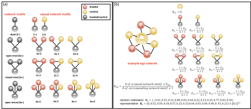
Figure 1: Illustration of causal network motif. (a) Examples of causal network motifs. Red indicates the node being treated, yellow indicates control, and grey indicates that it could be in treatment or control. The bottom node for each network network is the ego. The first patterns in each row are conventional network motifs without assignment conditions, or just called network motifs, followed by corresponding causal network motifs. Our causal network motif representation is constructed by dividing the count of a causal network motif by the count of the corresponding causal network motif. The labels below each network motif indicate the naming: for example, an open triad where one neighbor is treated is named 3o-1 (the second causal network motif of the third row). (b) Construction of causal network motif representation. This is an example of an ego network with treatment assignments and the corresponding causal network motif representation. Red indicates the node being treated, yellow indicates control, and grey indicates that it could be treatment or control.

Figure 1(a) illustrates our construction of causal network motif representation. The first dimension is the treatment assignment of unit $i$, i.e. $R_{i1}=Z_{i}$. For the rest of dimensions ($m>1$), we should first specify the network motifs and then causal network motifs. Each dimension ($m>1$) is the fraction of a causal network motif over the corresponding network motif.

$$R_{im}=\frac{\text{\# of a causal network motif}}{\text{\# of the corresponding network motif}}\text{ for }m>1.$$ (8)

This is the normalized number of causal network motifs over the total number of corresponding network motifs. For example, it could be the number of fully treated open triads (3o-2) over the number of all open triads (3o). Note that one major reason for us to construct in this way is to satisfy the representation invariance properties.

Remark 4.1

The mapping $g$ that corresponds to our causal network motif construction is representation invariant to $\bm{1}$ and $\bm{0}$.

Therefore, this property enables us to further estimate global average treatment effects under our framework.

When calculating network motifs at higher orders, it is typically computationally expensive – imagine that it is non-trivial to find the number of fully connected squares of a unit when they have thousands of neighbors. In this case, we can instead just randomly sample a small fraction of their neighbors and calculate the ratio of each causal network motif in the sampled network motifs. This ratio can be used to approximate the true ratio when a node has a very large degree and precise counts of motifs are infeasible.

Although our way of construction is empirically useful, it is not the only feasible one. One example is that we can instead define another other possible construction $R_{im}=\frac{1}{\text{\# of a causal network motif}}$ but it is not a representation invariant to $\bm{1}$ and $\bm{0}$.

Adjusting construction to satisfy positivity requirement. A core requirement of exposure mapping, or causal inference in general, is “positivity”. That is for

$$\mathbb{P}[\bm{R}_{i}\in\mathcal{R}_{k}]>0,\text{ for all }i\in\mathcal{N}\text{ and }k=1,2,\cdots,|\Delta|.$$ (9)

The rationale is that positivity can help with the Horvitz–Thompson estimator or the Hájek estimator with non-zero numerators. This is also part of the reason why we normalize the causal network motif representation by the corresponding number of network motifs. Consider using the count of each causal network motif as its elements; should a partition be chosen where the number of closed triads with fully treated neighbors exceeds 10, any units with fewer than 10 open triads would hold zero probability of inclusion in this partition.

When calculating each ${R}_{im}$ ($m>1$), we add some randomness — $U_{im}$ is i.i.d. draw from the continuous uniform distribution $\text{Unif}([0,1])$. In this way, for each ${R}_{im}$ where $m>1$, it has a full support within $[0,1]$. Therefore the actual causal network motif representation becomes

$$R_{im}=\frac{\text{\# of a causal network motif}+U_{im}}{\text{\# of corresponding network motif}+1}\quad\text{ for }m>1.$$ (10)

With this technique, we can address the issue of having a certain number of network motifs being zero, leading to zero-valued numerators in the causal network motif representation.

5 Machine Learning to Specify Exposure Mapping

We introduce two machine learning algorithms — decision trees and nearest neighbors — that can be used to construct a function $h$ that maps a causal network motif $\bm{R}_{i}$ to an exposure condition $\mathcal{R}$. The decision tree method focuses on partitioning the space of $[0,1]^{M}$ into disjoint subspaces, i.e., $\mathcal{R}_{1}\cup\mathcal{R}_{2}\cup\mathcal{R}_{3}\cup\cdots\cup\mathcal{R}_{|\Delta|}$, while the nearest neighbors method focuses on the two exposure conditions ($\mathcal{R}_{k_{1}},\mathcal{R}_{k_{0}}\in\Delta$) that contain fully treated and non-treated assignment conditions respectively to estimate the global treatment effect.

When choosing between the two approaches, it is important to consider the main goal of the modeling. The decision tree approach is better suited for learning a suitable exposure mapping function, while the nearest neighbors approach is better for estimating global average treatment effects. Although we can also estimate global average treatment effects via the tree-based approach, the nearest neighbors approach also has the added flexibility of being able to optimize its parameters to select the least biased estimator among multiple candidates.

5.1 Tree-Based Approach

We use decision trees to partition the space of the causal network motif representation, which is $[0,1]^{M}$, into multiple disjoint subspaces: $[0,1]^{M}=\mathcal{R}_{1}\cup\mathcal{R}_{2}\cup\mathcal{R}_{3}\cup\cdots\cup\mathcal{R}_{|\Delta|}$. We adapt the “exposure mapping” proposed by Aronow and Samii (2017), where units are categorized into a number of “leaves” in the decision tree. However, compared with conventional decision tree regression, we need to propose the following revisions. As this was part of the main contribution of the previous conference version Yuan et al. (2021), we only list the core ideas and leave the details in Appendix E:

1. Splitting rule: We propose two score functions to guide partitioning in decision trees: the t-statistic and the weighted sum of squares error (WSSE). These metrics are used to find the best partition score and split the node into child nodes. Constraints are introduced to prevent the tree from growing unnecessarily deep.

2. Honest splitting: Similar to Athey and Imbens (2016), we also aim to avoid overfitting the training set and the potential overestimation of differences. We do this by splitting all units into training and estimation sets. Then we use the training set for tree partitioning only and use the estimation set for calculating the mean and variance.

3. Inverse probability weighting: One essential difference, as noted in previous sections, is that we aim to estimate the average potential outcomes for each partition (exposure condition). This requires the use of inverse probability weighting methods such as HT or Hájek estimations.

The algorithm is implemented by recursion (see Algorithm 3 in Appendix E). Specifically, we have a procedure Split which is used to partition a given space in $[0,1]^{M}$. One can use Split($[0,1]^{M}$) to start the recursion algorithm. When the algorithm terminates, each leaf corresponds to an exposure condition ($\mathcal{R}$) and we then calculate $\hat{\mu}(\mathcal{R})$, the average potential outcome for an exposure condition $\mathcal{R}$.

In addition to estimating the average potential outcome, our approach can also be used to estimate the global average treatment effects. Since the mapping for causal network motif representation ($g$) is representation invariant to $\bm{z}=\bm{1}$ and $\bm{0}$, we can define $\bm{r}^{(1)}=g(\bm{1},\cdot)$ and $\bm{r}^{(0)}=g(\bm{0},\cdot)$ for all $i\in\mathcal{N}$. Then we just need to find the two leaves of the decision trees (i.e., exposure conditions) that contain $\bm{r}^{(1)}$ and $\bm{r}^{(0)}$ and compare the difference between $\hat{\mu}(\mathcal{R}_{k_{1}})$ and $\hat{\mu}(\mathcal{R}_{k_{0}})$ to estimate the global average treatment effect.

5.2 Nearest Neighbors Approach

Since the main goal of the tree-based algorithm is to specify exposure mapping, it does not necessarily find the two best specifications to represent and approximate the fully treated or non-treated scenarios. In many cases, an experimenter’s primary purpose is to estimate the global average treatment effect, such as the impact of updating their recommendation algorithm. We thus introduce the nearest neighbors approach. Similar to the tree-based approach, we require that exposure mapping $f$ is representation invariant to $\bm{z}=\bm{1}$ and $\bm{z}=\bm{0}$. Again, we denote $\bm{r}^{(1)}=g(\bm{1},\theta_{i})$ and $\bm{r}^{(0)}=g(\bm{0},\theta_{i})$ as they are the same for all $i\in\mathcal{N}$.

In the nearest neighbor approach, it is important to determine a distance metric $d$ (the distance between two representations $\bm{r}$ and $\bm{r}^{\prime}$) and the number of nearest neighbors $K$ (to $\bm{r}^{(1)}$ or $\bm{r}^{(0)}$) and in order to specify exposure conditions. The choice of distance metric and $K$ can greatly affect the accuracy of the estimation. We can represent the exposure mapping $h$ as a function of the distance metric $d$ and $K$, denoted as $h^{d,K}$. Therefore, we can rewrite $\mu^{f}$ as $\mu^{d,K}$ and $\tau^{f}$ as $\tau^{d,K}$ for the nearest neighbors approach.

To estimate the global average treatment effect, we should just focus on the two exposure conditions that contain the fully treated and non-treated scenarios respectively. Therefore,

$$h^{d,K}(\bm{r})=\begin{cases}\mathcal{R}_{k_{1}}&\bm{r}\text{ is of }K\text{ nearest neighbors of }\bm{r}^{(1)}\text{ under metric }d\\ \mathcal{R}_{k_{0}}&\bm{r}\text{ is of }K\text{ nearest neighbors of }\bm{r}^{(0)}\text{ under metric }d\\ \mathcal{R}_{\text{otw}}&\text{otherwise}\end{cases}$$

Given $\Delta=\{\mathcal{R}_{k_{1}},\mathcal{R}_{k_{0}},\mathcal{R}_{\text{otw}}\}$, we only need to compare $\mathcal{R}_{k_{1}}$ versus $\mathcal{R}_{k_{0}}$ to compute the global average treatment effect. We can estimate the global average treatment effect by $\hat{\tau}^{d,K}=\hat{\mu}^{d,K}(\mathcal{R}_{k_{1}})-\hat{\mu}^{d,K}(\mathcal{R}_{k_{0}})$ , We should also satisfy the positivity requirement for $\mathcal{R}_{k_{1}}$ and $\mathcal{R}_{k_{0}}$.

One challenge with the nearest neighbors approach is defining the distance metric between two vector representations in order to determine which units have closer representations ($\bm{R}_{i}$) to $\bm{r}^{(1)}$ or $\bm{r}^{(0)}$. We primarily use the regression coefficients distance metric for our main results. That is, we first directly regress the outcome ($Y$) on the $\bm{r}_{i}$ using a linear regression model, and then obtain the regression coefficients $\bm{\beta}$. We then define the distance metric as:

$$d_{\text{C}}(\bm{r},\bm{r}^{\prime})=||\bm{\beta}\circ\bm{\bm{r}}||_{1}$$ (11)

Here $\circ$ is the element-wise product and $||\bm{x}||_{1}$ is $\ell_{1}$ norm. In Appendix F we also discuss other metrics and compare them in our empirical section.

The next question is how to choose the optimal $K$. From Proposition 3.4, we know that the largest (smallest) estimator under non-negative (non-positive) interference assumption should be the least biased one. Therefore, we can search among a set of possible values of $K$ that satisfy the positivity requirement defined by Eq. (33), denoted by $\mathbb{K}$. For example, under non-negative interference assumption, we can then construct the following estimator:

$$\hat{\tau}^{*}=\text{max}_{K\in\mathbb{K}}\left(\hat{\mu}^{d,K}(\mathcal{R}_{k_{1}})-\hat{\mu}^{d,K}(\mathcal{R}_{k_{0}})\right)\leq\tau.$$ (12)

This means that such $K$ that leads to the largest estimator without violating the positivity requirement produces the least biased estimator.

In the example above, we know that there exists a $K\in\mathbb{K}$ that leads to a least biased estimator. Next, we show that when we have certain restrictions for the distance metric $d$, the smallest $K$ that satisfies the positivity requirement should be the least biased one. In order to describe these restrictions, we define a properly specified distance metric $d$:

Definition 5.1 (properly specified distance metric)

For all $\bm{z},\bm{z}^{\prime}\in\{0,1\}^{N}$, $\bm{r}_{i}=g(\bm{z},\theta)$ and $\bm{r}_{i}^{\prime}=g(\bm{z}^{\prime},\theta)$ for all $i\in\mathcal{N}$,

1. Under the non-negative interference assumption, distance metric $d$ is properly specified when for all $i\in\mathcal{N}$, if $d(\bm{r}^{(1)},\bm{r}_{i})\geq d(\bm{r}^{(1)},\bm{r}_{i}^{\prime})$ then $y_{i}(\bm{z})\leq y_{i}(\bm{z}^{\prime})$, and if $d(\bm{r}^{(0)},\bm{r}_{i})\geq d(\bm{r}^{(0)},\bm{r}_{i}^{\prime})$ then $y_{i}(\bm{z})\geq y_{i}(\bm{z}^{\prime})$.

2. Under the non-positive interference assumption, distance metric $d$ is properly specified when for all $i\in\mathcal{N}$, if $d(\bm{r}^{(1)},\bm{r}_{i})\geq d(\bm{r}^{(1)},\bm{r}_{i}^{\prime})$ then $y_{i}(\bm{z})\geq y_{i}(\bm{z}^{\prime})$, and if $d(\bm{r}^{(0)},\bm{r}_{i})\geq d(\bm{r}^{(0)},\bm{r}_{i}^{\prime})$ then $y_{i}(\bm{z})\leq y_{i}(\bm{z}^{\prime})$.

Intuitively, a properly specified distance metric should properly reflect the relationship of the potential outcome $y_{i}$ and the distance between causal network motif representations $\bm{r}_{i}$ versus $\bm{r}^{(1)}$ (or versus $\bm{r}^{(0)}$): when $\bm{r}_{i}$ is farther from $\bm{r}^{(1)}$ (or $\bm{r}^{(0)}$) according to distance metric $d$, the potential outcome $y_{i}$ should change monotonically. Note that this is also the core assumption of the nearest neighbors algorithm when it is used for prediction, which is the general purpose of the algorithm.

Under the assumption of a properly specified $d$, we can better justify the best choice of $K$:

Proposition 5.2

1. If we assume that interference is non-negative and we have a correctly defined distance metric $d$, as $K$ gets larger (within a range that maintains positivity), the expected value of $\hat{\tau}_{\text{HT}}^{d,K}$ reduces. Moreover, the difference between this expected value and the real effect, (or in other words, the bias of $\hat{\tau}_{\text{HT}}^{d,K}$ towards $\tau$), expands.

2. If we assume that interference is non-positive and we have a correctly defined distance metric $d$, as $K$ gets larger (within a range that maintains positivity), the expected value of $\hat{\tau}_{\text{HT}}^{d,K}$ grows. Moreover, the difference between this expected value and the real effect, (or in other words, the bias of $\hat{\tau}_{\text{HT}}^{d,K}$ towards $\tau$), also expands.

Proof. See Appendix A.3.

Here we discuss our intuition of this proposition. It is widely accepted that it is extremely challenging to perfectly correctly specify an exposure mapping function in real-world applications; thus it is unlikely to have an unbiased estimator of the global average treatment effect anyhow. However, by carefully designing the distance metric of the nearest neighbors algorithm, we can safely assume that the potential outcome $y_{i}$ has a monotonic trend as the representation $\bm{r}_{i}$ moves away from $\bm{r}^{(1)}$ (or $\bm{r}^{(0)}$). This implies that when we use a narrower region around $\bm{r}^{(1)}$ (or $\bm{r}^{(0)}$) to approximate the fully treated or non-treated scenario (i.e., $\mathcal{R}_{k_{1}}$ and $\mathcal{R}_{k_{0}}$ respectively), we can obtain a less biased estimation of the true average global treatment effect. In this case, when selecting $K$ for the $K$NN algorithm, it may be beneficial to choose a small value as long as the positivity requirement is empirically satisfied and the variance is acceptably small. This can help produce an estimator with a small bias from the global average treatment effect. Note that the monotonic trend regarding the variance is not necessarily guaranteed, though empirically it tends to decrease in $K$.

Algorithm 1 Implementation for the nearest neighbors algorithm

1:procedure NN($K$, $d$, $B$) $\triangleright$ $B$ is number of bootstraps

2:     Initialize $\bm{r}^{(1)}$ and $\bm{r}^{(0)}$ according to causal network motif construction $g$.

3:     Using nearest neighbors algorithm to find the $K$ units that have the $K$ smallest $d(\bm{r}^{(1)},\bm{R}_{i})$, whose region defines $\mathcal{R}_{k_{1}}$.

4:     Use Eq. (3) to compute $\hat{\mu}(\mathcal{R}_{k_{1}})$.

5:     for $b\in[1,B]$ do

6:         Compute Eq. (3) to compute $\hat{\mu}^{(b)}(\mathcal{R}_{k_{1}})$.

7:     end for

8:     Estimate $\widehat{\text{Var}}(\hat{\mu}(\mathcal{R}_{k_{1}}))$ with the bootstrap results

9:     Using nearest neighbors algorithm to find the $K$ units that have the $K$ smallest $d(\bm{r}^{(0)},\bm{R}_{i})$, whose region $\mathcal{R}_{k_{0}}$.

10:     Use Eq. (3) to compute $\hat{\mu}(\mathcal{R}_{k_{0}})$.

11:     for $b\in[1,B]$ do

12:         Compute Eq. (3) to compute $\hat{\mu}^{(b)}(\mathcal{R}_{k_{0}})$.

13:     end for

14:     Estimate $\widehat{\text{Var}}(\hat{\mu}(\mathcal{R}_{k_{0}}))$ with the bootstrap results

15:end procedure

Variance Estimation.

Estimating the variance in the presence of network interference can be challenging. In our empirical experiments, we mainly use bootstrapping for at least 500 replicates to estimate the variance of Hájek and HT estimators. Algorithm 2 presents the procedure ($B$ is the number of replicates). One can consider using 2.5th and 97.5th percentiles of the bootstrapping results to construct confidence intervals.

Algorithm 2 Variance estimation with bootstrapping.

1:for $b$ from $1$ to $B$ do

2:     Collect a random sample with replacement from the set $\mathcal{N}$, with indices $i^{b}_{1}$, $i^{b}_{2}$, $\cdots$, $i^{b}_{N}$. If the experiment is a cluster randomization, randomly sample at the cluster level.

3:     Compute $\hat{\mu}^{(b)}$ or $\hat{\tau}^{(b)}$ using $i^{b}_{1}$, $i^{b}_{2}$, $\cdots$, $i^{b}_{N}$ based on Eq (3).

4:end for

5:$\widehat{\text{Var}}(\hat{\mu})=\frac{1}{B}\sum_{b=1}^{B}{(\hat{\mu}^{(b)}-\bar{\mu})^{2}}$ where $\bar{\mu}=\frac{1}{B}\sum_{b=1}^{B}\hat{\mu}^{(b)}$.

6:$\widehat{\text{Var}}(\hat{\tau})=\frac{1}{B}\sum_{b=1}^{B}{(\hat{\tau}^{(b)}-\bar{\tau})^{2}}$ where $\bar{\tau}=\frac{1}{B}\sum_{b=1}^{B}\hat{\tau}^{(b)}$.

Alternatively, we can compute the variance in closed form using the methods described in Aronow and Samii (2017) for HT estimators and Taylor linearization for Hájek estimators (Särndal et al. 1992). This has the advantage of being more efficient, but may not be straightforward to apply to certain experimental designs, such as graph cluster randomization (Ugander et al. 2013, Eckles et al. 2016). To compute the $p$ value, we can use the percentiles from the bootstrapped results. We can also compute the exact $p$ value using the methods described in Athey et al. (2018). See Appendix B for more details.

6 Synthetic and Real-World Experiments

In this section, we present results on synthetic and real-world experiments to demonstrate the validity of our approach. For the synthetic experiments, we simulate the potential outcome function on a synthetic network based on Watts-Strogatz network (Watts and Strogatz 1998) and on a real-world network (Slashdot). These simulation settings enable us to compare the ground truth of the potential outcomes to the estimation of our approach. In order to demonstrate how our method applies to real-world experiments, we also include an experiment on Instagram’s 1-2 million users, where detailed network information is provided and individuals are randomly assigned to treatment or control with Bernoulli randomization.

6.1 Small-World Networks with Synthetic Potential Outcomes

Setup.

Since real-world data cannot provide full information about potential outcomes in all counterfactuals, solely using real-world experiments would be difficult to evaluate any causal inference method. Thus, we begin by using a synthetic network and generate potential outcomes.

The Watts-Strogatz network is a classical network model that captures important real-world network properties including clustering and six degrees of separation (Watts and Strogatz 1998). One important parameter in this model is the rewiring rate which belongs to $[0,1]$; it controls the randomness and the extent of clustering of the network. We chose a rewiring rate of $0.5$ which results in a diverse set of causal network motifs and helps illustrate the advantage of our approach compared to not accounting for motifs. Watts-Strogatz network has also been widely used in previous work on network interference, including Eckles et al. (2016) and Chin (2019). We generated the potential outcome functions for each node using the following function:

$$y_{i}(\bm{Z})=(1+X_{i})(1+Z_{i}+\sum_{j\in\mathcal{N}_{i}}w_{ij}Z_{j})+\varepsilon_{i}.$$ (13)

Here, $w_{ij}$ is the weight for each pair for relationship: we first compute the number of common friends between $i$ and $j$, denoted by $\text{cf}_{ij}$; then we compute $w_{ij}=\frac{(X_{j}+1)\text{cf}_{ij}}{\sum_{j\in\mathcal{N}_{i}}(X_{j}+1)\text{cf}_{ij}}$. This implies that neighbors sharing more mutual friends exert stronger interference. Pairs without mutual friends are presumed not to generate any interference. This further underscores the potential significance of closed network motifs (like closed triads or squares) in characterizing interference. $X_{i}$ is a binary covariate that interacts with the treatment assignments of both the ego nodes and other nodes. Here we assume that there are two types of nodes (e.g. different genders or other demographic groups) and that $X_{i}\sim\text{Bern}(0.5)$. The effect size and interference are in general larger when $X_{i}=1$, and the Gaussian noise is $\varepsilon_{i}\sim N(0,\frac{1}{16})$. The inclusion of $X_{j}$ denotes heterogeneous interference based on neighbors’ attributes. In other words, Group $X_{j}=1$ generally induces stronger interference spillage onto their neighbors compared to Group $X_{j}=0$. Note that this potential outcome adheres to the non-negative interference assumption.

In this synthetic data, when $Z_{i}=1$ for all $i\in\mathcal{N}$, the average potential outcome (or $\mu(\bm{1})$) equals $5.7$ when $Z_{i}=0$ for all $i\in\mathcal{N}$, the average potential outcome (or $\mu(\bm{0})$) equals $1.5$; therefore, the true global average treatment effect is $\tau=\mu(\bm{1})-\mu(\bm{0})=4.2$.

We evaluate two randomization approaches: Bernoulli randomization and graph cluster randomization (Ugander et al. 2013, Eckles et al. 2016). In the case of graph cluster randomization, we apply the standard Kernighan–Lin graph clustering algorithm (Kernighan and Lin 1970) recursively, yielding a total of 512 balanced (same-sized) graph clusters. For each $i\in\mathcal{N}$, we randomly assign the treatment $Z_{i}\sim\text{Bern}(0.5)$. As an illustration, we choose $Z_{i}$, proportion of treated neighbors (2-1), non-treated open triads (3o-0), treated open triads (3o-2), non-treated closed triads (3c-0), treated closed triads (3c-2), treated open triads (4o-3), and non-treated open triads (4o-0), as depicted in Figure 1. These causal network motifs demonstrate how each individual and their network neighborhood are exposed to treatments. Furthermore, we take into account the proportion of treated neighbors with $X_{j}=1$, namely 2-1(1), and proportion of treated neighbors with $X_{j}=0$ in our assessment, namely 2-1(0), aside from the proportion of treated neighbors (2-1). This addition helps to account for heterogeneous interference attributable to the attributes of $j$. Our analysis primarily focuses on 1-hop ego networks, although it is feasible to consider higher-order ego networks as well.

Tree Result.

We first present the results of the tree-based algorithm for this synthetic network in Figure 2. The tree is derived from the estimation set for the honest splitting purpose Athey and Imbens (2016). As shown in the upper panel, there are 14 exposure conditions for the Bernoulli randomization. We use leaf (i.e. an exposure condition) $\mathcal{R}_{5}$ as an illustrative example. If a unit is in control (left split), the fraction of fully-non-treated closed triad is smaller than 51% (left split), the fraction of fully-treated closed triad is greater than 32% (right split), and the fraction of treated neighbors with covariate ($X$) equal to 1 is greater than 56% (right split), it specifies a unique exposure condition $\mathcal{R}_{5}$, which exhibits the largest average potential outcome (3.71) among all exposure conditions under ego being controlled. This indicates that even if this unit is in the control group, if the majority of the closely embedded neighborhood is treated, and in particular those neighbors with $X_{j}=1$ are also mostly treated, their outcome would be the largest even though they do not receive the treatment. This has implications, for instance, for how to utilize this heterogeneous peer effect and network structure to promote more adoptions when the number of treatments is limited. The result for cluster randomization yields fewer (five) exposure conditions, as shown in the lower panel of Figure 2. This is due to the inter-dependence in their treatment assignments as well as the smaller variation in causal network motifs under this randomization. Thus, cluster randomization may not always be ideal for revealing interference heterogeneity as Bernoulli randomization does.

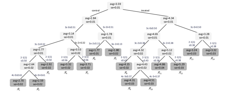
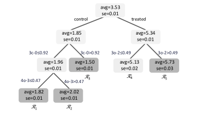
Figure 2: Tree-algorithm results for the Watts-Strogatz synthetic experiment: (upper) Bernoulli randomization and (lower) graph cluster randomization. Each leaf corresponds to an exposure condition. The decision path towards each leaf indicates the subspace of $[0,1]^{M}$ that corresponds to exposure condition. We use training sets to construct the trees and estimation sets to estimate the average potential outcomes and their standard errors. Codes of causal network motifs are marked in Fig. 1. “2-1(1)” indicates the fraction of treated neighbors with covariate equal to 1.

The tree results can also be used to estimate the global average treatment effect – in this case we need to find the two special exposure conditions that include the fully treated or fully non-treated counterfactual worlds, respectively (in other words, including $\bm{r}^{(0)}$ and $\bm{r}^{(1)}$, respectively). In the Bernoulli randomization, $\mathcal{R}_{6}$ and $\mathcal{R}_{12}$ contain $\bm{r}^{(0)}$ and $\bm{r}^{(1)}$ respectively, with an average potential outcomes of $5.290(\pm 0.030)$ and $1.771(\pm 0.014)$. Note that their difference ($3.519$) is much larger than simply comparing the treatment and the control groups ($4.335-2.842=1.493$), and this is a less biased estimation of the global average treatment effect ($4.2$). Similarly, for the cluster randomization, $\mathcal{R}_{3}$ and $\mathcal{R}_{5}$ contain $\bm{r}^{(0)}$ and $\bm{r}^{(1)}$ respectively, with average potential outcomes of $5.732(\pm 0.026)$ and $1.824(\pm 0.013)$. This further reduces the bias of estimating the global average treatment effect.

We also compare our approach with the fractional $q$ neighborhood exposure mapping. Using this approach produces four exposure conditions only. As shown in Figure A.3, less information about heterogeneity of network interference is revealed when only the dyad-level features are used. For example, under Bernoulli randomization, exposure conditions $\mathcal{R}_{1}$ and $\mathcal{R}_{2}$ are the only two exposure conditions under control. The fraction of treated neighbors can only detect much smaller differences in the average potential outcomes compared to our approach. It also has inferior performance in terms of estimating global average treatment effects. For instance, under Bernoulli randomization, this approach can estimate the global average treatment effect as $4.614-2.380=2.235$, which is much smaller and biased than using the causal network motifs we proposed to use (3.519 for our estimation in Bernoulli case, and 4.200 for the true effect).

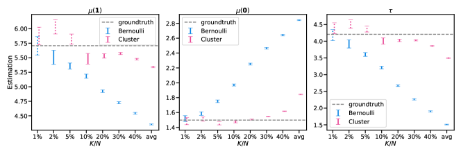
Figure 3: Estimation Utilizing Nearest Neighbor Approach for Watts-Strogatz synthetic experiment: The figure showcases Hájek estimators employing Bernoulli and graph cluster randomization schemes. The $x$-label $K/N$ represents the fraction of the number of nodes used in the nearest neighbor exposure condition relative to the entire population. Error bars depict standard errors, wherein the dotted error bars indicate estimates that do not meet the positivity requirement. The dashed gray lines represent the ground truth, reflecting the average potential outcomes for fully treated ($\mu(\bm{1})$) or non-treated ($\mu(\bm{0})$) groups, as well as the global treatment effect ($\tau$). The label “avg” denotes the approach of calculating average outcomes for treatment and/or control groups.

Nearest Neighbors Result.

Next, we showcase our nearest neighbors approach, with an emphasis on estimating the global average treatment effect. We set $K$ to represent a fraction of the total number of nodes, as depicted in Figure 3. If $K$ is too small and fails to satisfy the positivity requirement, estimations should be disregarded, indicated by dashed error bars in the figure.

We evaluate the average potential outcomes for the fully treated ($\mu(\bf{1})$), fully non-treated ($\mu(\bf{0})$) scenarios, and then estimate the global average treatment ($\tau$). Initial observations from the Bernoulli randomization reveal an increasing bias with $K$, denoted by a decreasing trend in the estimations of $\mu(\bf{1})$ and $\tau$, and an increasing trend for $\mu(\bf{0})$. This observation aligns with the conclusions from Proposition 5.2. At the same time, an inverse relationship is observed between the increasing $K$ and decreasing variance, reflecting a growing number of units contributing to the estimation and highlighting an intriguing bias-variance trade-off. One practical method for selecting the optimal value of $K$ consists of defining an upper limit for the variance, and then choosing the smallest $K$ that not only produces a variance less than this threshold but also meets the positivity requirement. This strategy helps identify the least biased estimator that maintains a reasonably small variance (under the monotonic interference assumption).

We also apply the nearest neighbors approach to graph cluster randomization. Note in this setting that specific nodes are less likely to belong to two particular exposure conditions, $\mathcal{R}_{k_{1}}$ and $\mathcal{R}_{k_{0}}$, due to their clustering with closely embedded neighbors (such nodes tend to exhibit features like 3c-2 that are closer to either 1 or 0). The bias-variance trade-off identified in the Bernoulli randomization also applies to cluster randomization: When the positivity requirement is met, an increase in $K$ results in a decrease in variance, but a concurrent increase in bias. Interestingly, merging these two methods—our approach and cluster randomization—can enhance the precision of the estimation beyond what our approach achieves alone. For instance, $K=\lfloor 10\%N\rfloor$ is the smallest $K$ that satisfies positivity, and it exhibits less bias than the least biased estimation in the Bernoulli case, while maintaining a similar variance. This further underscores the potential benefits of combining different randomization approaches. The results also suggest that our approach can be effectively incorporated with graph cluster randomization.

We also compare our approach with fractional $q$ neighborhood exposure. Essentially, fractional $q$ neighborhood exposure is equivalent to our approach with the fraction of treated neighbors only. For a fair comparison, we compare our approach with the fractional $q$ neighborhood exposure when we keep $K$ the same. As shown in Figure A.2, we find that using our approach has a significantly smaller bias than the fractional $q$ neighborhood approach, and the variance is more or less similar. This further demonstrates the need to use motifs beyond simply counting the fraction of treated neighbors.

We also demonstrate the importance of a well-defined distance metric. For instance, the bias from a metric based on regression coefficients is generally less than that of an “identical” metric proposed in Appendix F, implying the necessity to weigh different dimensions differently. Moreover, we also show that the Hájek estimator generally outperforms the Horvitz–Thompson estimator in terms of variance, although their biases are comparable. See Appendix G.1 for more details.

6.2 Instagram Tutorial on the Avatars Product

Setup.

Next, to demonstrate the capability of our approach on a real-world randomized experiment, we apply it to a 1-2 million user experiment on the Instagram platform, which was aimed at improving the user experience for a new product called Instagram Avatars. Instagram Avatars was introduced in February 2022  as a way for users to better express themselves in the digital world. The Avatar product allows users to create a 3D digital version of themselves and use it in stories and direct messages (DMs), referred to as Instagram Direct. In order to help users better understand how to use the new Avatars product, Instagram ran an A/B test in August 2022 that experimented with a new interactive experience. The experience raises awareness about the Avatars product by testing a flow that displays all possible Avatars and shows users how to customize them. After users are shown a grid of different Avatars, it immediately prompts them to share with others. Users in the treatment group were exposed to this tutorial, which guides users on Avatar creation and facilitates sharing while users in the control group did not get the tutorial experience.

We limit the analysis to users who were exposed to the experiment (i.e. active Instagram users between August 29 and September 27, 2022), resulting in a balanced sample of 1-2 million users. Note that all data was de-identified and analyzed in aggregate; this part of the analysis was done internally at Meta. Users in the experiment were randomly split into treatment and control conditions under Bernoulli randomization. We examine the impact of the new exit user experience on whether users are more likely to use Avatars in Instagram Direct, which is coded as a binary outcome variable. When doing the naive analysis on September 27 between users who had been previously exposed to the tutorial versus those that did not, we estimate a treatment effect of $\hat{\tau}$=0.10% ($\pm$ 0.03%) on an absolute scale. This means that the tutorial was effective in getting more users to use Avatars.

However, interference may exist in this experiment which may mislead the estimation of the global average treatment effect. For example, even if a user is in the control condition, if they have more neighbors in the treatment condition, they may be more aware of the Avatar product and more likely to use it. Therefore, naively comparing treatment and control conditions may underestimate the true global average treatment effect or provide incorrect insights into the impact of this experiment. In order to address possible interference, we propose using causal network motif features (bootstrap 500 times for variance) based on the mutual follow graph on Instagram among users in the A/B test. We employ the fraction of treated neighbors (2-1), fully treated closed triads (3c-2), fully non-treated closed triads (3c-2) as causal network motifs as an illustration.

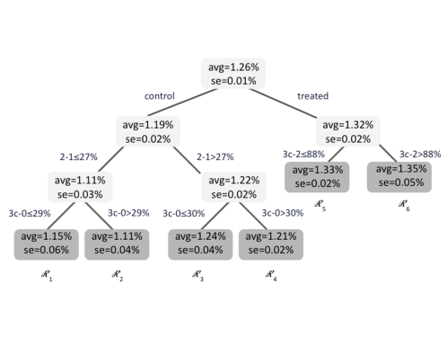
Figure 4: Tree-algorithm results for the Instagram real-world test. Each leaf corresponds to an exposure condition. The decision path towards each leaf indicates the subspace of $[0,1]^{M}$ that corresponds to exposure condition. We use training sets to construct the trees and estimation sets to estimate the average potential outcomes and their standard errors. Codes of causal network motifs are marked in Fig. 1.

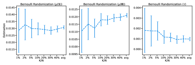
Figure 5: Estimation Utilizing Nearest Neighbor Approach for the Instagram Experiment: The figure showcases Hájek estimators employing Bernoulli randomization. The $x$-label $K/N$ represents the fraction of the number of nodes used in the nearest neighbor exposure condition relative to the entire population. Error bars depict standard errors, wherein the dotted error bars indicate estimates that do not meet the positivity requirement. The label “avg” denotes the approach of calculating average outcomes for treatment and/or control groups.

Tree Result.

We first illustrate the tree-based result for the estimation split in Figure 4. From this result, we find a large degree of heterogeneity of network interference among the control group as the control group has four exposure conditions. When a user is in the control and their neighbors are mostly in the control group (2-1 $<27\%$) and a sufficiently large fraction of closed triads are fully non-treated (3c-0 $>29\%$), the average potential outcome ($1.11\%\pm 0.04\%$) is the smallest (exposure condition $\mathcal{R}_{2}$. By contrast, when the ego is in the control group but $>27\%$ their neighbors are treated and a sufficiently small fraction of closed triads are fully non-treated (3c-0 $\leq 30\%$), the average potential outcome is much larger ($1.24\%\pm 0.04\%$; exposure condition $\mathcal{R}_{3}$). These results show that even when a person is in the control group, their treated neighbors, especially highly clustered neighbors, still play an important role in prompting them to use it. By contrast, for the treatment group, there seems not to be a strong interference pattern.

Nearest Neighbor Result.

We next illustrate the nearest neighbor results in Figure 5. Using the regression coefficients metric as an example, we observe an increasing pattern for $\hat{\mu}(\bf{0})$ in $K$ in the middle panel when ignoring the first two estimations with very large variance. This is consistent with the observation from the tree-based result where we find more treated neighbors and closed triads predict a higher probability for control users to use the product. By contrast, a clear monotonic trend is not observed for the treatment group, meaning that interference is much smaller for treatment group users (left panel). Based on the result when $K=\lfloor 5\%N\rfloor$ from the last panel of Figure 5, we learn that the estimation of ${\tau}$ could even be biased by more than 75% if we simply contrast the averages of the treatment versus control groups (under the monotonic interference assumption). This further supports the capability of our approach to reduce bias for the global average treatment effect estimation.

6.3 Two Additional Setups

Slashdot Social Network.

We next use the public network data from Slashdot, a technology-related news website known for its specific user community, provided by Leskovec et al. (2009). This network has 82,168 nodes and 582,533 edges, with a long-tailed degree distribution. We generate the same potential outcomes with the Watts-Strogatz network and present the estimation results in Appendix G.2. These results show that the network structure should not affect our conclusion.

Rural Insurance Experiment.

As another simple illustrative example, we also apply our approach to the publicly available data provided by Cai et al. (2015), a randomized experiment for rice farmers in rural China. The experiment included 4,832 households across 185 villages, meaning that it is not a large-scale experiment typically conducted by digital platforms. Note that the original experiment was already under-powered to explore significant interference heterogeneity. The application of our approach is used for illustrative purposes only (see Appendix G.3).

7 Concluding Remarks

A/B testing is a prevalent technique for guiding product iterations on user-centric platforms. Nevertheless, interference often poses challenges to the validity of such methods. To tackle these challenges, we propose a two-part approach: firstly, we suggest the use of “causal network motifs” to describe intricate interference patterns; secondly, we devise a machine learning framework to analyze network interference algorithmically. Our theoretical analysis and empirical results from synthetic and real-world A/B tests substantiate the validity of our approach.

Our study distinguishes itself amidst the burgeoning literature on analysis-based network interference methods. Primarily, our use of causal network motifs offers a practical means of defining features (variables) within the frameworks proposed by Chin (2019), Awan et al. (2020), Cortez et al. (2022a), Qu et al. (2021), Belloni et al. (2022), enabling these models to account for complex network structures. Furthermore, in contrast to works such as Sussman and Airoldi (2017), Chin (2019), Cortez et al. (2022a), Yu et al. (2022) that rely on linearity or additivity assumptions and analytical approaches, we employ machine learning techniques, providing an alternative perspective to algorithmically characterize network interference. Likewise, while Qu et al. (2021) proposes an approach for analyzing heterogeneity in interference, a combination of their approach on accounting for neighbors’ covariates with our focus on network structure potentially further improves estimation accuracy. This was demonstrated in our Watts Strogatz and Slashdot synthetic experiments.

In addition, while other related works such as Awan et al. (2020) and Belloni et al. (2022). offer a matching-based perspective to address network interference, their primary focus is observational settings rather than the online A/B testing settings. In addition, their primary focus does not lie in the determination of exposure mapping functions or the estimation of the global average treatment effect as we do. Furthermore, our use of machine learning aligns with the application found in Leung and Loupos (2022)’s Graph Neural Network (GNN) framework. However, our approach emphasizes an interpretable solution, designed to be directly employed in large-scale experimentation settings, with a highlight on the qualitative understanding of network interference.

Our methodology offers three promising applications for practitioners. First, integrating our approach into experimentation systems allows for a retrospective review of past A/B tests, providing insights into network interference patterns and facilitating more accurate estimation of global average treatment effects. Second, the insights (i.e., exposure conditions defined by the algorithm) obtained from our method can aid in the optimization of both design-based (e.g., redefining network structures for graph cluster randomization) and analysis-based strategies (e.g., defining more appropriate exposure mapping) for future experiments. Finally, our approach can assist in identifying the exposure conditions that yield the most beneficial outcomes, thereby enabling optimal distribution of interventions, in areas such as targeting for product promotions.

Our work suggests several paths for further exploration. First, the adaptation of our method to observational studies can be a promising avenue, although it would require careful consideration of external factors, particularly when randomized experiments are not viable. Moreover, our approach may be suitable for situations where only parts of a network are observable or even in non-network contexts. This flexibility may also prove useful when access to user data or specific network attributes is restricted. Finally, our approach could be integrated with the modern influence maximization problem in social networks, a field that currently emphasizes the modeling of the diffusion process, rather than placing greater focus on causality.

Appendix

A Proofs

A.1 Proof for Lemma 6

Proof.

$$\begin{split}\mathbbm{E}[\hat{\mu}_{\text{HT}}^{f}(\mathcal{R})]&=\frac{1}{N}\mathbbm{E}[\sum_{i}\frac{Y_{i}\mathbbm{1}[\bm{R}_{i}\in\mathcal{R}]}{\mathbb{P}[\bm{R}_{i}\in\mathcal{R}]}]\\ &=\sum_{\bm{z}\in\{0,1\}^{N}}\frac{1}{N}\sum_{i}\frac{y_{i}(\bm{z})\mathbbm{1}[g(\bm{z},\theta_{i})\in\mathcal{R}]\mathbb{P}[\bm{Z}=\bm{z}]}{\mathbb{P}[g(\bm{Z},\theta_{i})\in\mathcal{R}]}\\ &=\frac{1}{N}\mathbbm{E}[y_{i}(\bm{Z})|\bm{R}_{i}\in\mathcal{R}]=\frac{1}{N}\sum_{i\in\mathcal{N}}\mathbbm{E}[y_{i}(\bm{Z})|g(\bm{Z},\theta_{i})\in\mathcal{R}]={\mu}^{f}(\mathcal{R}).\end{split}$$ (14)

A.2 Proof for Proposition 3.4

Proof.

1. $$\tau^{f}=\mathbbm{E}[\hat{\tau}_{\text{HT}}^{f}] =\mathbbm{E}\left[\frac{\sum_{i}Y_{i}w_{i}(\mathcal{R}_{k_{1}})}{N}-\frac{\sum_{i}Y_{i}w_{i}(\mathcal{R}_{k_{0}})}{N}\right]$$ (15)

   $$=\mathbbm{E}\left[\frac{\sum_{i}y_{i}^{f}(\mathcal{R}_{k_{1}})w_{i}(\mathcal{R}_{k_{1}})}{N}-\frac{\sum_{i}y_{i}^{f}(\mathcal{R}_{k_{0}})w_{i}(\mathcal{R}_{k_{0}})}{N}\right]$$ (16)

   $$=\mathbbm{E}\left[\frac{\sum_{i}y_{i}(\bm{1})w_{i}(\mathcal{R}_{k_{1}})}{N}-\frac{\sum_{i}y_{i}(\bm{0})w_{i}(\mathcal{R}_{k_{0}})}{N}\right]$$ (17)

   $$=\frac{1}{N}\sum_{i}\left(y_{i}(\bm{1})-y_{i}(\bm{0})\right)=\tau$$ (18)

   The third equality is derived from the assumption that the correct specification assumption. The fourth equality is from the fact that $\mathbbm{E}\left[\frac{\mathbbm{1}[\bm{R}_{i}\in\mathcal{R}]}{\mathbbm{P}[\bm{R}_{i}\in\mathcal{R}]}\right]=1$.

2. $$\tau^{f}=\mathbbm{E}[\hat{\tau}_{\text{HT}}^{f}] =\mathbbm{E}\left[\frac{\sum_{i}Y_{i}w_{i}(\mathcal{R}_{k_{1}})}{N}-\frac{\sum_{i}Y_{i}w_{i}(\mathcal{R}_{k_{0}})}{N}\right]$$ (19)

   $$=\mathbbm{E}\left[\frac{\sum_{i}y_{i}(\bm{Z})w_{i}(\mathcal{R}_{k_{1}})}{N}-\frac{\sum_{i}y_{i}(\bm{Z})w_{i}(\mathcal{R}_{k_{0}})}{N}\right]$$ (20)

   $$\leq\mathbbm{E}\left[\frac{\sum_{i}y_{i}(\bm{1})w_{i}(\mathcal{R}_{k_{1}})}{N}-\frac{\sum_{i}y_{i}(\bm{0})w_{i}(\mathcal{R}_{k_{0}})}{N}\right]$$ (21)

   $$=\frac{1}{N}\sum_{i}\left(y_{i}(\bm{1})-y_{i}(\bm{0})\right)=\tau$$ (22)

   The inequality is from the non-negative interference assumption. The third equality is from the fact that $\mathbbm{E}\left[\frac{\mathbbm{1}[\bm{R}_{i}\in\mathcal{R}]}{\mathbbm{P}[\bm{R}_{i}\in\mathcal{R}]}\right]=1$.

3. This is symmetric to proof 2 except that the sign should be “$\geq$” and non-positive interference should be assumed.

A.3 Proof for Proposition 5.2

Proof. Here we only provide detailed proof for non-negative interference assumption and the proof for non-positive interference assumption is symmetric.

Consider two possible values for $K$: $\bar{K}$ and $\underaccent{\bar}{K}$ ($\underaccent{\bar}{K}\leq\bar{K}$). Note that we should only consider $K$ that lead to exposure conditions that satisfy the positivity requirement. Let $\mathcal{R}^{d,\bar{K}}_{k_{1}}$ and $\mathcal{R}^{d,\bar{K}}_{k_{0}}$ denote the exposure conditions corresponding to the fully treated or non-treated scenarios defined by the $\bar{K}$ nearest neighbors. Let $\mathcal{R}^{d,\underaccent{\bar}{K}}_{k_{1}}$ and $\mathcal{R}^{d,\underaccent{\bar}{K}}_{k_{0}}$ denote the exposure conditions corresponding to the fully treated or non-treated scenarios defined by the $\underaccent{\bar}{K}$ nearest neighbors.

$$\begin{split}\mathbbm{E}[\hat{\tau}_{\text{HT}}^{d,\bar{K}}]-\mathbbm{E}[\hat{\tau}_{\text{HT}}^{d,\underaccent{\bar}{K}}]=\frac{1}{N}\sum_{i\in\mathcal{N}}\left(\mathbbm{E}[y_{i}(\bm{Z})|g(\bm{Z},\theta_{i})\in\mathcal{R}^{d,\bar{K}}_{k_{1}}]-\mathbbm{E}[y_{i}(\bm{Z})|g(\bm{Z},\theta_{i})\in\mathcal{R}^{d,\underaccent{\bar}{K}}_{k_{1}}]\right)\\ -\frac{1}{N}\sum_{i\in\mathcal{N}}\left(\mathbbm{E}[y_{i}(\bm{Z})|g(\bm{Z},\theta_{i})\in\mathcal{R}^{d,\bar{K}}_{k_{0}}]-\mathbbm{E}[y_{i}(\bm{Z})|g(\bm{Z},\theta_{i})\in\mathcal{R}^{d,\underaccent{\bar}{K}}_{k_{0}}]\right)\end{split}$$ (23)

We know $\mathcal{R}^{d,\underaccent{\bar}{K}}_{k_{1}}\subseteq\mathcal{R}^{d,\bar{K}}_{k_{1}}$ according to the nature of nearest neighbors algorithm, i.e. we would include more units but do not exclude as we increase $K$. Therefore we can separate $\mathcal{R}^{d,\bar{K}}_{k_{1}}$ into $\mathcal{R}^{d,\underaccent{\bar}{K}}_{k_{1}}$ and $\mathcal{R}^{d,\bar{K}}_{k_{1}}\setminus\mathcal{R}^{d,\underaccent{\bar}{K}}_{k_{1}}$ and then we derive:

$$\frac{1}{N}\sum_{i\in\mathcal{N}}\left(\mathbbm{E}[y_{i}(\bm{Z})|g(\bm{Z},\theta_{i})\in\mathcal{R}^{d,\bar{K}}_{k_{1}}]-\mathbbm{E}[y_{i}(\bm{Z})|g(\bm{Z},\theta_{i})\in\mathcal{R}^{d,\underaccent{\bar}{K}}_{k_{1}}]\right)$$ (24)

$$= \frac{1}{N}\sum_{i\in\mathcal{N}}\left(p\mathbbm{E}[y_{i}(\bm{Z})|g(\bm{Z},\theta_{i})\in\mathcal{R}^{d,\underaccent{\bar}{K}}_{k_{1}}]+(1-p)\mathbbm{E}[y_{i}(\bm{Z})|g(\bm{Z},\theta_{i})\in\mathcal{R}^{d,\bar{K}}_{k_{1}}\setminus\mathcal{R}^{d,\underaccent{\bar}{K}}_{k_{1}}]-\mathbbm{E}[y_{i}(\bm{Z})|g(\bm{Z},\theta_{i})\in\mathcal{R}^{d,\underaccent{\bar}{K}}_{k_{1}}]\right)$$ (25)

$$= \frac{1}{N}\sum_{i\in\mathcal{N}}(1-p)\left(\mathbbm{E}[y_{i}(\bm{Z})|g(\bm{Z},\theta_{i})\in\mathcal{R}^{d,\bar{K}}_{k_{1}}\setminus\mathcal{R}^{d,\underaccent{\bar}{K}}_{k_{1}}]-\mathbbm{E}[y_{i}(\bm{Z})|g(\bm{Z},\theta_{i})\in\mathcal{R}^{d,\underaccent{\bar}{K}}_{k_{1}}]\right)$$ (26)

where $\mathbbm{P}[g(\bm{Z},\theta_{i})\in\mathcal{R}^{d,\underaccent{\bar}{K}}_{k_{1}}|g(\bm{Z},\theta_{i})\in\mathcal{R}^{d,\bar{K}}_{k_{1}}]=p$ and $\mathbbm{P}[g(\bm{Z},\theta_{i})\in\mathcal{R}^{d,\bar{K}}_{k_{1}}\setminus\mathcal{R}^{d,\underaccent{\bar}{K}}_{k_{1}}|g(\bm{Z},\theta_{i})\in\mathcal{R}^{d,\bar{K}}_{k_{1}}]=1-p$. The first equality follows the law of total expectation. The second quality is derived from merging the first and third terms.

Again by the nature of nearest neighbor algorithm, for all $\bm{r}\in\mathcal{R}^{d,\bar{K}}_{k_{1}}\setminus\mathcal{R}^{d,\underaccent{\bar}{K}}_{k_{1}}$ and $\bm{r}^{\prime}\in\mathcal{R}^{d,\underaccent{\bar}{K}}_{k_{1}}$, $d(\bm{r}^{(1)},\bm{r})\geq d(\bm{r}^{(1)},\bm{r}^{\prime})$. This is because the $\underaccent{\bar}{K}$ nearest neighbors of $\bm{r}^{(1)}$ should be a subset of the $\bar{K}$ nearest neighbors of $\bm{r}^{(1)}$. As we assume that $d$ is properly specified, we can convert the inequality of distance metric $d$ to the potential outcome $y_{i}$, i.e.,

$$\mathbbm{E}[y_{i}(\bm{Z})|g(\bm{Z},\theta_{i})\in\mathcal{R}^{d,\bar{K}}_{k_{1}}\setminus\mathcal{R}^{d,\underaccent{\bar}{K}}_{k_{1}}]\leq\mathbbm{E}[y_{i}(\bm{Z})|g(\bm{Z},\theta_{i})\in\mathcal{R}^{d,\underaccent{\bar}{K}}_{k_{1}}].$$ (27)

Then by combining this with Eq. (26), we have

$$\frac{1}{N}\sum_{i\in\mathcal{N}}\mathbbm{E}[y_{i}(\bm{Z})|g(\bm{Z},\theta_{i})\in\mathcal{R}^{d,\bar{K}}_{k_{1}}]\leq\frac{1}{N}\sum_{i\in\mathcal{N}}\mathbbm{E}[y_{i}(\bm{Z})|g(\bm{Z},\theta_{i})\in\mathcal{R}^{d,\underaccent{\bar}{K}}_{k_{1}}].$$ (28)

Similarly, we can derive

$$\frac{1}{N}\sum_{i\in\mathcal{N}}\mathbbm{E}[y_{i}(\bm{Z})|g(\bm{Z},\theta_{i})\in\mathcal{R}^{d,\bar{K}}_{k_{0}}]\geq\frac{1}{N}\sum_{i\in\mathcal{N}}\mathbbm{E}[y_{i}(\bm{Z})|g(\bm{Z},\theta_{i})\in\mathcal{R}^{d,\underaccent{\bar}{K}}_{k_{0}}].$$ (29)

Therefore, we can conclude $\mathbbm{E}[\hat{\tau}_{\text{HT}}^{d,\bar{K}}]\leq\mathbbm{E}[\hat{\tau}_{\text{HT}}^{d,\underaccent{\bar}{K}}]$.

Therefore, $\mathbbm{E}[\hat{\tau}_{\text{HT}}^{d,{K}}]$ decreases in $K$.

Moreover, we learn from Proposition 3.4 that $\mathbbm{E}[\hat{\tau}_{\text{HT}}^{d,\bar{K}}]\leq\tau$ and $\mathbbm{E}[\hat{\tau}_{\text{HT}}^{d,\underaccent{\bar}{K}}]\leq\tau$ under the non-negative interference assumption. Therefore, $|\mathbbm{E}[\hat{\tau}_{\text{HT}}^{d,\bar{K}}]-\tau|\geq|\mathbbm{E}[\hat{\tau}_{\text{HT}}^{d,\underaccent{\bar}{K}}]-\tau|$, i.e. the bias of $\mathbbm{E}[\hat{\tau}_{\text{HT}}^{d,{K}}]$ increases in $K$.

B Additional details for inference

Here we discuss how to compute the exact $p$ value through randomization inference (Imbens and Rubin 2015). In practice, one important test is to examine whether two exposure conditions have significantly different average potential outcomes. This also applies to the estimation of global average treatment effect.

Here we assume that there are two exposure conditions $\mathcal{R}$ and $\mathcal{R}^{\prime}$ and we want to test the null hypothesis that there is no difference in potential outcomes between $\mathcal{R}$ and $\mathcal{R}^{\prime}$. That is, for all $\bm{z},\bm{z}^{\prime}\in\{0,1\}^{N}$ such that $f(\bm{z},\theta_{i})=\mathcal{R}$ and $f(\bm{z}^{\prime},\theta_{i})=\mathcal{R}^{\prime}$ for all $i\in\mathcal{N}$, $y_{i}(\bm{z})=y_{i}(\bm{z}^{\prime})$.

There are multiple ways to construct the test statistic. Here we just give one example: one may construct the following test statistic for the HT estimator:

$$T(\bm{y}(\bm{Z}),\bm{Z})=\left\lvert\sum_{i\in\mathcal{F}}\left(\frac{y_{i}(\bm{Z})\mathbbm{1}[\bm{R}_{i}\in\mathcal{R}]}{\mathbbm{P}[\bm{R}_{i}\in\mathcal{R}]}-\frac{y_{i}(\bm{Z})\mathbbm{1}[\bm{R}_{i}\in\mathcal{R}^{\prime}]}{\mathbbm{P}[\bm{R}_{i}\in\mathcal{R}^{\prime}]}\right)\right\rvert.$$ (30)

Here $\mathcal{F}$ is the focal set defined by Athey et al. (2018). Since we rely on $n$-hop neighborhood interference assumption, $\mathcal{F}$ is a subset of all population $\mathcal{N}$ such that (1) for all $i\in\mathcal{F}$, either $\bm{R}_{i}\in\mathcal{R}$ or $\bm{R}_{i}\in\mathcal{R}^{\prime}$; (2) their $n$-hop ego networks do not overlap. In other words, we want to find a focal set such that we can independently manipulate the assignments in their ego networks and randomize them into either $\mathcal{R}$ or $\mathcal{R}^{\prime}$. In this way, there would exist a set of random assignments, denoted by $\mathbb{Z}(\mathcal{F},\mathcal{R},\mathcal{R}^{\prime})$, under which computation of Equation (30) is feasible. We can compute the $p$ value of this null hypothesis by

$$p\text{-value}=\frac{\sum_{\bm{z}\in\mathbb{Z}(\mathcal{F},\mathcal{R},\mathcal{R}^{\prime})}\mathbbm{1}[T(y(\bm{z}),\bm{z})\geq T(y(\bm{Z}),\bm{Z})]\mathbb{P}(\bm{Z}=\bm{z})}{\sum_{\bm{z}\in\mathbb{Z}(\mathcal{F},\mathcal{R},\mathcal{R}^{\prime})}\mathbb{P}(\bm{Z}=\bm{z})}.$$ (31)

In practice, this can be done by independent draws from $\mathbb{Z}(\mathcal{F},\mathcal{R},\mathcal{R}^{\prime})$ for at least 500 replicates.

C Additional Details for Estimating General Probability of Exposure

As mentioned in the main text, one challenge is to compute the probability of a unit belonging to a specific exposure condition, referred to as the “general probability of exposure.” This probability is used in both the Horvitz–Thompson estimator and Hájek estimator. We use Monte Carlo simulation to estimate this probability. Specifically, we randomly assign treatments ($\bm{Z}$) for $B$ replicates, which generate the empirical probability of the event that $\bm{R}_{i}$ belongs to $\mathcal{R}$, that is $\bm{R}_{i}^{(1)},\bm{R}_{i}^{(1)},\cdots,\bm{R}_{i}^{(B)}$. That is for unit $i$,

$$\hat{\mathbbm{P}}[\bm{R}_{i}\in\mathcal{R}]=\frac{\sum_{b=1}^{B}\mathbbm{1}[\bm{R}_{i}^{(b)}\in\mathcal{R}]}{B+1}.$$ (32)

The “$+1$” in the denominator is to avoid zero-valued empirical probability when we use Hájek or Horvitz-Thompson estimators.

D Additional Details for Representation Invariance

Here we further discuss how representation invariance is satisfied when the randomness term $\bm{U}_{i}$ is added. In order to ensure representation invariance hold again we can allow $g$ to take the randomness $\bm{U}_{i}$ as the input, i.e., $\bm{R}_{i}=g(\bm{Z},\bm{U}_{i},\theta_{i})$. We can set the value of $\bm{U}_{i}$ for all $i\in\mathcal{R}$ properly: for $\mathcal{R}_{k_{1}}$, we set $\bm{U}_{i}$ to be 1 for dimensions that count full treatment conditions (e.g. 2-1, 3c-2 and 3o-2) and set $\bm{U}_{i}$ to be 0 for dimensions that count full control conditions (e.g. 2-0, 3c-0 and 3o-0), which is denoted by $\bm{U}^{(1)}$; and we can similarly find $\bm{U}^{(0)}$ for the other exposure condition $\mathcal{R}_{k_{0}}$. In this way, we still have $g(\bm{1},\bm{U}^{(1)},\theta_{i})=g(\bm{1},\bm{U}^{(1)},\theta_{j})\in\mathcal{R}_{k_{1}}$ for all $i\neq j$ and $g(\bm{0},\bm{U}^{(0)},\theta_{i})=g(\bm{0},\bm{U}^{(0)},\theta_{j})\in\mathcal{R}_{k_{0}}$ for all $i\neq j$; and thus representation invariance still holds.

E Additional Details for Tree-Based Result

Here we discuss technical details for the tree-based algorithm:

1. (Positivity in empirical general probability of exposure). Positivity ensures that all units have a non-zero probability of being in an exposure condition (Rubin 2005). The tree algorithm should not split a node if such splitting would lead to any child node (corresponding to an exposure condition) where there is a unit that violates the positivity requirement. Since $\mathbb{P}[\bm{R}_{i}\in\mathcal{R}]$ is often not solvable analytically, we use Monte Carlo to approximate it (denoted by $\hat{\mathbb{P}}[\bm{R}_{i}\in\mathcal{R}]$). Moreover, we adjust the positivity requirement to non-trivial probability, which allows very few units to have zero or near-zero probability; positive real numbers $\delta$ and $\epsilon$ introduce a small bias but allow partitioning more features.

   $$\frac{1}{N}\sum_{i\in\mathcal{N}}\mathbbm{1}[\hat{\mathbb{P}}[\bm{R}_{i}\in\mathcal{R}]\leq\epsilon]\leq\delta$$ (33)

   It means that the fraction of units with $\hat{\mathbb{P}}[\bm{R}_{i}\in\mathcal{R}]\leq\epsilon$ is smaller than $\delta$.

2. (Splitting rule) Here we introduce two score functions for the tree algorithm to determine when to further split given a current node (represented by $\mathcal{R}$) into its left and right children (denoted by $\mathcal{R}_{l}$ and $\mathcal{R}_{r}$ respectively): $t$ statistic and the weighted sum of squares error (WSSE).

   For the $t$ statistic, we define

   $$\text{Score}_{t}(\mathcal{R}_{l},\mathcal{R}_{r})=\frac{|\hat{\mu}(\mathcal{R}_{l})-\hat{\mu}(\mathcal{R}_{r})|}{\sqrt{\widehat{\text{Var}}\left(\hat{\mu}(\mathcal{R}_{l})-\hat{\mu}(\mathcal{R}_{r})\right)}}$$ (34)

   Here $\hat{\mu}$ can be either Hájek or HT estimator. It is essential the $t$ statistic for the test for the null hypothesis that the average potential outcomes for the two results exposure conditions are equal. A large $t$ statistic indicates that such a split would lead to two resulting exposure conditions with significantly different average potential outcomes.

   In addition to the $t$ statistic, we can also use weighted SSE as the split criterion. We define

   $$\begin{split}\text{Score}_{s}(\mathcal{R}_{l},\mathcal{R}_{r})=&\text{WSSE}(\mathcal{R}_{l}\cup\mathcal{R}_{r})-\\ &\left(\frac{\left(\sum_{i}\mathbbm{1}[\bm{R}_{i}\in\mathcal{R}_{l}]\right)\text{WSSE}(\mathcal{R}_{l})+\left(\sum_{i}\mathbbm{1}[\bm{R}_{i}\in\mathcal{R}_{r}]\right)\text{WSSE}(\mathcal{R}_{r})}{\sum_{i}{\mathbbm{1}[\bm{R}_{i}\in\left(\mathcal{R}_{l}\cup\mathcal{R}_{r}\right)]}}\right),\\ &\text{ where }\text{WSSE}(\mathcal{R})=\sum_{i\in\mathcal{N},\bm{R}_{i}\in\mathcal{R}}\frac{1}{\hat{\mathbb{P}}[\bm{R}_{i}\in\mathcal{R}]}(Y_{i}-\hat{\mu}(\mathcal{R}))^{2}.\end{split}$$ (35)

   which means the reduction in WSSE after we split $\mathcal{R}$ further into the two disjoint subsets $\mathcal{R}_{l}$ and $\mathcal{R}_{r}$ and calculate their average weighted by the number of units in each subset.

   Note that Hájek estimator can be derived by minimizing weighted sum of squared errors given a candidate exposure condition, which corresponds to a subset of $[0,1]^{M}$ (denoted by $\mathcal{R}$). In other words, $\hat{\mu}_{\text{H\'{a}jek}}(\mathcal{R})$ can be determined by the following equation:

   $$\hat{\mu}_{\text{H\'{a}jek}}(\mathcal{R})=\text{arg}\min_{y}\sum_{i\in\mathcal{N},\bm{R}_{i}\in\mathcal{R}}\frac{1}{\mathbb{P}[\bm{R}_{i}\in\mathcal{R}]}(Y_{i}-y)^{2}.$$ (36)

   For both the $t$ statistic and WSSE scores, the goal is to find the optimal partition score of the node $\mathcal{R}$ to two child nodes $\mathcal{R}_{l}^{*},\mathcal{R}_{r}^{*}$ (and ultimately leaves):

   $$\begin{split}\mathcal{R}_{l}^{*},\mathcal{R}_{r}^{*}=&\text{argmax}_{\mathcal{R}_{l},\mathcal{R}_{r}:\mathcal{R}_{l}\cup\mathcal{R}_{r}=\mathcal{R}\text{ and }\mathcal{R}_{l}\cap\mathcal{R}_{r}=\emptyset}\text{Score}(\mathcal{R}_{l},\mathcal{R}_{r})\\ &\text{ s.t. }\text{Score}(\mathcal{R}_{l},\mathcal{R}_{r})\geq\gamma\text{ and }\sum_{i}\mathbbm{1}[\bm{R}_{i}\in\mathcal{R}_{l}]\geq\kappa\text{ and }\sum_{i}\mathbbm{1}[\bm{R}_{i}\in\mathcal{R}_{r}]\geq\kappa.\end{split}$$ (37)

   In this equation, $\gamma$ is a hyper-parameter used to require non-trivial increases in the score function. Similar to conventional decision trees, we can also set the minimum leaf size ($\kappa$) to prevent the tree from growing unnecessarily deep. Both parameters can be tuned using cross validation in the training set. If the constraints cannot be satisfied, $(\mathcal{R}^{*}_{l},\mathcal{R}^{*}_{r})$ is an empty set and the algorithm would not further split $\mathcal{R}$.

3. (Honest splitting) When estimating variance of the tree results, the algorithm tends to choose a cutoff such that the objective is minimized; however, it may overfit the training set, leading to an improper cutoff that produces overestimation of the difference between the average potential outcomes of the two child nodes. We thus split all units into training and estimation sets — the training set is used for tree partitioning only whereas a separate estimation set is used for estimating the mean and variance. This is a common approach to correcting estimations in causal inference (Athey and Imbens 2016, Künzel et al. 2019).

Algorithm 3 Implementation for the tree-based algorithm

1:procedure Split($\mathcal{R}$)

2:     $\mathcal{R}^{*}_{l},\mathcal{R}^{*}_{r}=\emptyset$

3:     Compute $\hat{\mu}(\mathcal{R})$ and its variance using estimation set

4:     Initialize $\text{Score}^{*}$

5:     for $m\in[1,M]$ do

6:         for $i\in\mathcal{N}$ do

7:              $\theta\leftarrow R_{im}$

8:              $\mathcal{R}_{l}\leftarrow\{j|R_{jm}\leq\theta\And\bm{R}_{j}\in\mathcal{R}\}$

9:              $\mathcal{R}_{r}\leftarrow\{j|{R}_{jm}>\theta\And\bm{R}_{j}\in\mathcal{R}\}$

10:              if Eq. (33) and conditions in Eq. (37) are true for both $\mathcal{R}_{l}$ and $\mathcal{R}_{r}$  then

11:                  Compute Score($\mathcal{R}_{l}$, $\mathcal{R}_{\text{r}}$) using training set

12:                  if Score($\mathcal{R}_{l}$, $\mathcal{R}_{r}$) ¿ Score^∗ then

13:                       $\mathcal{R}_{l}^{*}\leftarrow\mathcal{R}_{l}$

14:                       $\mathcal{R}_{r^{*}}\leftarrow\mathcal{R}_{r}$

15:                       $\text{Score}^{*}\leftarrow\text{Score}(\mathcal{R}_{l},\mathcal{R}_{r})$

16:                  end if

17:              end if

18:         end for

19:     end for

20:     if $\mathcal{R}_{l}^{*}\neq\emptyset$ and $\mathcal{R}_{r}^{*}\neq\emptyset$ then

21:         Split($\mathcal{R}_{l}^{*}$)

22:         Split($\mathcal{R}_{r}^{*}$)

23:     else

24:         Add new exposure condition $\mathcal{R}$ to the self of all exposure conditions $\Delta$.

25:     end if

26:end procedure

Algorithm 3 details the procedure of the tree-based algorithm.

F Additional Details for the Nearest Neighbors Approach

Here we discuss the two distance metrics used in the nearest neighbors approach:

• Identical weights. Since all dimensions of the representation are in $[0,1]$, it can be natural if we simply treat each dimension with equal weight.

  $$d_{\text{I}}(\bm{r},\bm{r}^{\prime})=||\bm{r}-\bm{r}^{\prime}||_{1}$$ (38)

• Regression coefficients. We can directly regress the outcome ($Y$) on the $\bm{r}_{i}$ using OLS. In this way, we construct a linear model for predicting the outcome by the causal motif representations. Say $\bm{\beta}$ is the regression coefficient, then we define the metric as follows:

  $$d_{\text{C}}(\bm{r},\bm{r}^{\prime})=||\bm{\beta}\circ\bm{\bm{r}}||_{1}$$ (39)

  Note $\circ$ is the element-wise product and $||\bm{x}||_{1}$ is $\ell_{1}$ norm. Intuitively, the dimension of the causal motif representation that is more predictive of the outcome would be scaled up, meaning that even a small discrepancy between $\bm{r}$ and $\bm{r}^{\prime}$ on those important dimensions would have a large impact on the distance.

G Additional Details for Experiment Results

G.1 Additional Details for Watts-Strogatz Network Experiment

Comparisons Between Distance Metrics.

First, we evaluate the efficacy of the two distance metrics proposed in our study. The identical distance metric, due to its inability to discern varying levels of importance among different dimensions of representation, often falls short. As observed in Figure A.1, the regression coefficient distance metric generally provides a more accurate and less biased estimation of the true effect. This finding corroborates our decision to predominantly use the regression coefficient distance metric throughout our study. In practical applications, it might be beneficial to incorporate more nuanced distance metric learning techniques to enhance performance. However, such explorations extend beyond the scope of our current investigation.

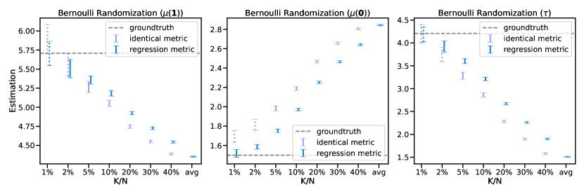
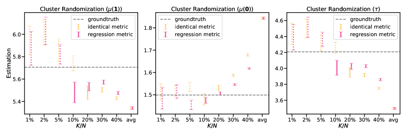
Figure A.1: Estimation Utilizing Nearest Neighbor Approach: The figure showcases Hájek estimators employing Bernoulli (upper) and graph cluster randomization (lower) schemes, with the identical distance metric or regression coefficient distance metric. The $x$-label $K/N$ represents the fraction of the number of nodes used in the nearest neighbor exposure condition relative to the entire population. Error bars depict standard errors, wherein the dotted error bars indicate estimates that do not meet the positivity requirement. The dashed gray lines represent the ground truth, reflecting the average potential outcomes for fully treated ($\mu(\bm{1})$) or non-treated ($\mu(\bm{0})$) groups, as well as the global treatment effect ($\tau$). The label “avg” denotes the approach of calculating average outcomes for treatment and/or control groups.

Comparisons with Fractional $q$ Neighborhood Exposure Mapping.

We establish a baseline comparison with the fractional $q$ neighborhood exposure mapping. Essentially, implementing fractional $q$ neighborhood exposure mapping is similar to our approach, albeit restricted to using the fraction of treated neighbors as the only feature. In order to ensure a fair comparison, we maintain the same $K$ value and assess the bias and variance between the fractional $q$ exposure mapping and our methodology.

Using Bernoulli randomization as an illustration, we depict in Figure A.2 that our approach and fractional $q$ neighborhood exposure mapping produce similar variance levels across all $K$ values. We observe that the bias of the estimator derived from our approach is considerably lower than that of the fractional $q$ neighborhood exposure mapping. This outcome underscores the advantage of utilizing intricate causal network motifs to capture complex network micro-patterns, thereby enabling a more accurate reflection of varied interference patterns in controlled experiments.

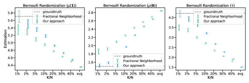
Figure A.2: Estimation Utilizing Nearest Neighbor Approach and Comparing Fractional $q$ Neighborhood Exposure Mapping versus Our Approach: The figure showcases Hájek estimators employing Bernoulli scheme, with the regression coefficient distance metric. The $x$-label $K/N$ represents the fraction of the number of nodes used in the nearest neighbor exposure condition relative to the entire population. Error bars depict standard errors, wherein the dotted error bars indicate estimates that do not meet the positivity requirement. The dashed gray lines represent the ground truth, reflecting the average potential outcomes for fully treated ($\mu(\bm{1})$) or non-treated ($\mu(\bm{0})$) groups, as well as the global treatment effect ($\tau$). The label “avg” denotes the approach of calculating average outcomes for treatment and/or control groups.

We also present the tree-based results using dyadic features only in Figure A.3. For instance, under Bernoulli randomization, we have only the exposure conditions $\mathcal{R}_{1}$ and $\mathcal{R}_{2}$. The proportion of treated neighbors can only distinguish differences to the smaller extent of $0.714$, a much smaller power than that in Figure 2. This also yields subpar outcomes in the estimation of global average treatment effects.

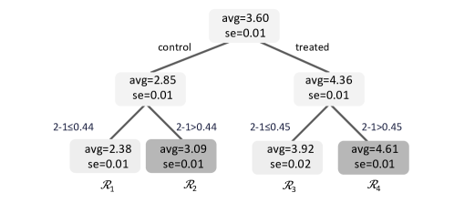
Figure A.3: Tree-algorithm results for the fractional $q$ neighborhood exposure mapping for Watts-Strogatz synthetic experiment (equivalent to using dyadic features only). Each leaf corresponds to an exposure condition. The decision path towards each leaf indicates the subspace of $[0,1]^{M}$ that corresponds to exposure condition. We use training sets to construct the trees and estimation sets to estimate the average potential outcomes and their standard errors. Codes of causal network motifs are marked in Fig. 1.

Horvitz–Thompson Estimator.

Finally, we present the results for the Horvitz–Thompson estimator. We use the nearest neighbors results as an illustration though the tree results are consistent. The results in the main text focuses on Hájek estimator because it is empirically “wise” by sacrificing a tiny amount of bias for a great variance reduction (Eckles et al. 2016, Khan and Ugander 2021). We present the result for Horvitz–Thompson estimator in Figure A.4. These tables show that, in general, the standard errors of the Horvitz-Thompson estimators are more than twice as large as those of the Hájek estimators. When the positivity requirement is satisfied, the difference between the Hájek and HT estimators is much smaller than the standard errors. The tree-based algorithm also yields a similar conclusion with the result of Hájek in the main text.

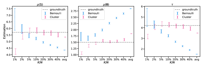
Figure A.4: Estimation Utilizing Nearest Neighbor Approach: The figure showcases Horvitz–Thompson estimators employing Bernoulli and graph cluster randomization schemes, with the regression coefficient distance metric. The $x$-label $K/N$ represents the fraction of the number of nodes used in the nearest neighbor exposure condition relative to the entire population. Error bars depict standard errors, wherein the dotted error bars indicate estimates that do not meet the positivity requirement. The dashed gray lines represent the ground truth, reflecting the average potential outcomes for fully treated ($\mu(\bm{1})$) or non-treated ($\mu(\bm{0})$) groups, as well as the global treatment effect ($\tau$). The label “avg” denotes the approach of calculating average outcomes for treatment and/or control groups.

G.2 Additional Details for the Slashdot Experiment

In this section, we analyze public network data from Slashdot, a news website renowned for its specific user community, as provided by Leskovec et al. (2009). The degree distribution of this network is presented in Figure A.5. The network comprises 82,168 nodes and 582,533 edges.

Figure A.5: Degree rank plot for the Slashdot network

Notably, unlike the Watts-Strogatz network, the Slashdot network exhibits a long-tailed degree distribution. We employed the same potential outcome functions as used in the Watts-Strogatz network and applied our methods to this real-world network. For our experiments, both Bernoulli and graph cluster randomizations (with 512 clusters) were conducted. Here $\mu(\bm{1})=6.0$, $\mu(\bm{0})=1.5$, and $\tau=4.5$.

Nearest neighbors results are presented in Figure A.6. As illustrated in the figures, all the primary conclusions drawn from the Watts-Strogatz network are applicable here. For example, a smaller value of $K$ results in less biased estimation, albeit with a larger variance. Additionally, integrating our approach with graph cluster randomization yields the least biased estimation. It is worth noting that in comparison to the Watts-Strogatz model, where the degree distribution is less skewed, a smaller value of $K$ seems to violate the positivity requirement more easily here. This is because nodes with a larger degree may be less likely to present a representation that closely resembles the fully treated or non-treated representations (much less likely to become a nearest neighbor).

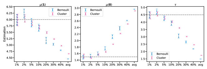
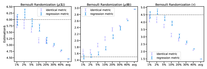
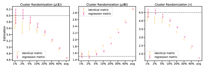
Figure A.6: Nearest Neighbor Estimation Results for the Slashdot Network. The x-label, $K/N$, denotes the fraction of nodes used in the nearest neighbor exposure condition relative to the total population. Error bars represent standard errors, with dotted bars indicating estimates that do not satisfy the positivity requirement. The dashed gray lines depict the ground truth, signifying the average potential outcomes for fully treated ($\mu(\bm{1})$) or non-treated ($\mu(\bm{0})$) groups, as well as the global treatment effect ($\tau$). The label “avg” refers to the method of calculating average outcomes for treatment and/or control groups.

G.3 Additional Details for the Rural China Insurance Adoption Network with Real-World Outcomes

As mentioned in the main text, we also use rural insurance experiment conducted by Cai et al. (2015) as another example. Cai et al. (2015) conducted a randomized experiment to introduce a new weather insurance policy for rice farmers in rural China. The experiment included 4,832 households across 185 villages. In order to understand the value of social networks for insurance understanding and adoption, the spillover effect was measured by informing a random subset of farmers on the rest of the farmers. The random assignment consisted of two waves: slightly less than half of the subjects were in the first wave, and the rest were in the second wave. In both waves, households (units) were randomized and assigned to treatment and control groups with Bernoulli randomization, where only the treatment group households received intensive introduction to the insurance. The analysis evaluated the impact on farmers’ understanding of the insurance benefits and whether they were more likely to adopt the insurance. The authors used survey data to collect network relationships among households.

Since the original paper found that the spillover pattern was fundamentally different between the first and the second stages, we separate the analyses for these two waves. While the original paper considered interference via the fraction of treated friends, we consider a more fine-grained analysis of how those friends are connected via causal network motifs. As an illustration, we select causal network motifs with the proportion of treated friends (2-1), the proportions of fully treated closed triad (3c-2).

Cai et al. (2015) found that the spillover pattern was different between the first and second waves. For the first wave, they only highlighted the difference in means between the treatment and control groups, but not spillover effects. For the second wave, the authors did not find a significant average treatment effect, but detected strong spillover effects from the units who were treated in the first wave.

We apply our tree-based approach to this experiment data. As shown in the left panel of Figure A.7, again, the first wave has a strong treatment effect. Among those treated, the average potential outcome is larger if a person has a large fraction of treated neighbors ($>$35%). For the right panel, the second wave participants no longer exhibit significant differences between those treated versus non-treated. Instead, our algorithm specifies the exposure mapping by the fraction of treated neighbors in the first wave. If this fraction is greater than 59%, the average potential outcome is larger than otherwise. Note that a small number of exposure conditions is expected, as the sample size is not comparable to what digital platforms typically perform experiments on.

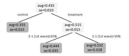
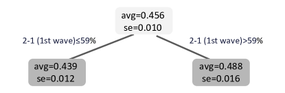
Figure A.7: Tree-algorithm results for the Watts-Strogatz synthetic experiment. Each leaf corresponds to an exposure condition. The decision path towards each leaf indicates the subspace of $[0,1]^{M}$ that corresponds to exposure condition. We use training sets to construct the trees and estimation sets to estimate the average potential outcomes and their standard errors. Codes of causal network motifs are marked in Fig. 1. The left and right panels are the results for the first and second waves respectively.

We next employ the nearest neighbors approach. We present the results of estimating $\mu(\bm{1})$ and $\mu(\bm{0})$, respectively. Again we split the analysis into the first and second waves in the left and right panels of Figure A.8, respectively. Most selected $K$ values satisfy the positivity requirement, except when $K$ is too small (indicated by dashed error bars and supposedly disregarded). For both waves, we observe that the $\hat{\mu}(\mathcal{R}_{k_{1}})$ appears to have a decreasing trend, whereas we do not observe a clear trend for $\hat{\mu}(\mathcal{R}_{k_{0}})$. If $K$ is large enough, it is close to simply taking averages of treated and non-treated samples. Regarding the global average treatment effect, estimations for both the first and second waves are larger than simply taking the average between treatment and control groups. This appears to be consistent with the results from previous studies such as (Chin 2019). However, since this is a small-sample network experiment compared to experiments on most online platforms with over millions of users, variance is large in these estimations.

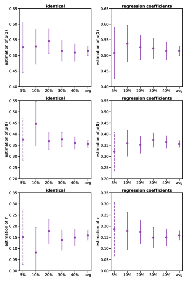
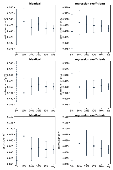
Figure A.8: The nearest neighbors result for the experiment of (Cai et al. 2015). The left panel (purple error bars) is the first wave result and the right panel (navy error bars) is the second wave result. Error bars represent standard errors. Dashed purple or navy error bars mean that less than 99% of units of non-zero estimated empirical general probability of exposure (violation of positivity).

References

- Aral and Nicolaides (2017) Aral S, Nicolaides C (2017) Exercise contagion in a global social network. Nature Communications 8(1):1–8.
- Aral and Van Alstyne (2011) Aral S, Van Alstyne M (2011) The diversity-bandwidth trade-off. American Journal of Sociology 117(1):90–171.
- Aral and Walker (2012) Aral S, Walker D (2012) Identifying influential and susceptible members of social networks. Science 337(6092):337–341.
- Aral and Walker (2014) Aral S, Walker D (2014) Tie strength, embeddedness, and social influence: A large-scale networked experiment. Management Science 60(6):1352–1370.
- Aronow et al. (2021) Aronow PM, Eckles D, Samii C, Zonszein S (2021) Spillover effects in experimental data. Advances in Experimental Political Science 289:319.
- Aronow and Samii (2017) Aronow PM, Samii C (2017) Estimating average causal effects under general interference, with application to a social network experiment. The Annals of Applied Statistics .
- Athey et al. (2018) Athey S, Eckles D, Imbens GW (2018) Exact p-values for network interference. Journal of the American Statistical Association 113(521):230–240.
- Athey and Imbens (2016) Athey S, Imbens G (2016) Recursive partitioning for heterogeneous causal effects. Proceedings of the National Academy of Sciences .
- Awan et al. (2020) Awan U, Morucci M, Orlandi V, Roy S, Rudin C, Volfovsky A (2020) Almost-matching-exactly for treatment effect estimation under network interference. International Conference on Artificial Intelligence and Statistics, 3252–3262 (PMLR).
- Bajari et al. (2021) Bajari P, Burdick B, Imbens GW, Masoero L, McQueen J, Richardson T, Rosen IM (2021) Multiple randomization designs. arXiv preprint arXiv:2112.13495 .
- Bakshy et al. (2014) Bakshy E, Eckles D, Bernstein MS (2014) Designing and deploying online field experiments. Proceedings of the 23rd International Conference on World Wide Web, 283–292.
- Bargagli-Stoffi et al. (2020) Bargagli-Stoffi FJ, Tortu C, Forastiere L (2020) Heterogeneous treatment and spillover effects under clustered network interference. arXiv preprint arXiv:2008.00707 .
- Basse and Airoldi (2018) Basse GW, Airoldi EM (2018) Model-assisted design of experiments in the presence of network-correlated outcomes. Biometrika 105(4):849–858.
- Basse et al. (2019) Basse GW, Feller A, Toulis P (2019) Randomization tests of causal effects under interference. Biometrika 106(2):487–494.
- Belloni et al. (2022) Belloni A, Fang F, Volfovsky A (2022) Neighborhood adaptive estimators for causal inference under network interference. arXiv preprint arXiv:2212.03683 .
- Bland (2004) Bland JM (2004) Cluster randomised trials in the medical literature: two bibliometric surveys. BMC Medical Research Methodology 4(1):1–6.
- Bojinov and Gupta (2022) Bojinov I, Gupta S (2022) Online experimentation: Benefits, operational and methodological challenges, and scaling guide .
- Bojinov et al. (2022) Bojinov I, Simchi-Levi D, Zhao J (2022) Design and analysis of switchback experiments. Management Science .
- Bowers et al. (2013) Bowers J, Fredrickson MM, Panagopoulos C (2013) Reasoning about interference between units: A general framework. Political Analysis 97–124.
- Boyarsky et al. (2023) Boyarsky A, Namkoong H, Pouget-Abadie J (2023) Modeling interference using experiment roll-out. arXiv preprint arXiv:2305.10728 .
- Brennan et al. (2022) Brennan J, Mirrokni V, Pouget-Abadie J (2022) Cluster randomized designs for one-sided bipartite experiments. Advances in Neural Information Processing Systems 35:37962–37974.
- Cai et al. (2015) Cai J, De Janvry A, Sadoulet E (2015) Social networks and the decision to insure. American Economic Journal: Applied Economics 7(2):81–108.
- Candogan et al. (2023) Candogan O, Chen C, Niazadeh R (2023) Correlated cluster-based randomized experiments: Robust variance minimization. Management Science .
- Centola (2010) Centola D (2010) The spread of behavior in an online social network experiment. Science .
- Centola and Macy (2007) Centola D, Macy M (2007) Complex contagions and the weakness of long ties. American Journal of Sociology 113(3):702–734.
- Chin (2019) Chin A (2019) Regression adjustments for estimating the global treatment effect in experiments with interference. Journal of Causal Inference 7(2).
- Cortez et al. (2022a) Cortez M, Eichhorn M, Yu CL (2022a) Exploiting neighborhood interference with low order interactions under unit randomized design. arXiv preprint arXiv:2208.05553 .
- Cortez et al. (2022b) Cortez M, Eichhorn M, Yu CL (2022b) Graph agnostic estimators with staggered rollout designs under network interference. arXiv preprint arXiv:2205.14552 .
- Diamantopoulos et al. (2020) Diamantopoulos N, Wong J, Mattos DI, Gerostathopoulos I, Wardrop M, Mao T, McFarland C (2020) Engineering for a science-centric experimentation platform. Proceedings of the ACM/IEEE 42nd International Conference on Software Engineering: Software Engineering in Practice, 191–200.
- Eckles et al. (2016) Eckles D, Karrer B, Ugander J (2016) Design and analysis of experiments in networks: Reducing bias from interference. Journal of Causal Inference 5(1).
- Forastiere et al. (2021) Forastiere L, Airoldi EM, Mealli F (2021) Identification and estimation of treatment and interference effects in observational studies on networks. Journal of the American Statistical Association 116(534):901–918.
- Gallagher and Eliassi-Rad (2008) Gallagher B, Eliassi-Rad T (2008) Leveraging label-independent features for classification in sparsely labeled networks: An empirical study. Proceedings of the Workshop on Social Network Mining and Analysis, 1–19 (Springer).
- Granovetter (1973) Granovetter MS (1973) The strength of weak ties. American Journal of Sociology 78(6):1360–1380.
- Hagiu and Wright (2015) Hagiu A, Wright J (2015) Marketplace or reseller? Management Science 61(1):184–203.
- Harshaw et al. (2023) Harshaw C, Sävje F, Eisenstat D, Mirrokni V, Pouget-Abadie J (2023) Design and analysis of bipartite experiments under a linear exposure-response model. Electronic Journal of Statistics 17(1):464–518.
- Holtz et al. (2020) Holtz D, Lobel R, Liskovich I, Aral S (2020) Reducing interference bias in online marketplace pricing experiments. arXiv preprint arXiv:2004.12489 .
- Hu et al. (2022) Hu Y, Li S, Wager S (2022) Average direct and indirect causal effects under interference. Biometrika .
- Hudgens and Halloran (2008) Hudgens MG, Halloran ME (2008) Toward causal inference with interference. Journal of the American Statistical Association 103(482):832–842.
- Imbens and Rubin (2015) Imbens GW, Rubin DB (2015) Causal inference in statistics, social, and biomedical sciences (Cambridge University Press).
- Johari et al. (2022) Johari R, Li H, Liskovich I, Weintraub GY (2022) Experimental design in two-sided platforms: An analysis of bias. Management Science .
- Kernighan and Lin (1970) Kernighan BW, Lin S (1970) An efficient heuristic procedure for partitioning graphs. The Bell System Technical Journal 49(2):291–307.
- Khan and Ugander (2021) Khan S, Ugander J (2021) Adaptive normalization for ipw estimation. arXiv preprint arXiv:2106.07695 .
- Kim and Fernandez (2017) Kim M, Fernandez RM (2017) Strength matters: Tie strength as a causal driver of networks’ information benefits. Social Science Research 65:268–281.
- Kohavi et al. (2013) Kohavi R, Deng A, Frasca B, Walker T, Xu Y, Pohlmann N (2013) Online controlled experiments at large scale. Proceedings of the 19th ACM SIGKDD International Conference on Knowledge Discovery and Data Mining, 1168–1176.
- Kohavi et al. (2020) Kohavi R, Tang D, Xu Y (2020) Trustworthy online controlled experiments: A practical guide to A/B testing (Cambridge University Press).
- Koning et al. (2022) Koning R, Hasan S, Chatterji A (2022) Experimentation and start-up performance: Evidence from A/B testing. Management Science 68(9):6434–6453.
- Kramer et al. (2014) Kramer AD, Guillory JE, Hancock JT (2014) Experimental evidence of massive-scale emotional contagion through social networks. Proceedings of the National Academy of Sciences 111(24):8788–8790.
- Künzel et al. (2019) Künzel SR, Sekhon JS, Bickel PJ, Yu B (2019) Metalearners for estimating heterogeneous treatment effects using machine learning. Proceedings of the National Academy of Sciences 116(10):4156–4165.
- Leskovec et al. (2009) Leskovec J, Lang KJ, Dasgupta A, Mahoney MW (2009) Community structure in large networks: Natural cluster sizes and the absence of large well-defined clusters. Internet Mathematics 6(1):29–123.
- Leung (2022) Leung MP (2022) Causal inference under approximate neighborhood interference. Econometrica 90(1):267–293.
- Leung and Loupos (2022) Leung MP, Loupos P (2022) Unconfoundedness with network interference. arXiv preprint arXiv:2211.07823 .
- Li et al. (2022) Li H, Zhao G, Johari R, Weintraub GY (2022) Interference, bias, and variance in two-sided marketplace experimentation: Guidance for platforms. Proceedings of the ACM Web Conference 2022, 182–192.
- Lyu et al. (2022) Lyu D, Yuan Y, Wang L, Wang X, Pentland A (2022) Investigating and modeling the dynamics of long ties. Communications Physics 5(1):1–9.
- Mahalanobis (1936) Mahalanobis PC (1936) On the generalized distance in statistics (National Institute of Science of India).
- Manski (2013) Manski CF (2013) Identification of treatment response with social interactions. The Econometrics Journal 16(1):S1–S23.
- Milo et al. (2002) Milo R, Shen-Orr S, Itzkovitz S, Kashtan N, Chklovskii D, Alon U (2002) Network motifs: simple building blocks of complex networks. Science 298(5594):824–827.
- Munro et al. (2021) Munro E, Wager S, Xu K (2021) Treatment effects in market equilibrium. arXiv:2109.11647 .
- Pollmann (2020) Pollmann M (2020) Causal inference for spatial treatments. arXiv preprint arXiv:2011.00373 .
- Pouget-Abadie et al. (2018) Pouget-Abadie J, Mirrokni V, Parkes DC, Airoldi EM (2018) Optimizing cluster-based randomized experiments under monotonicity. Proceedings of the 24th ACM SIGKDD International Conference on Knowledge Discovery & Data Mining, 2090–2099.
- Pouget-Abadie et al. (2019) Pouget-Abadie J, Saint-Jacques G, Saveski M, Duan W, Ghosh S, Xu Y, Airoldi EM (2019) Testing for arbitrary interference on experimentation platforms. Biometrika 106(4):929–940.
- Qu et al. (2021) Qu Z, Xiong R, Liu J, Imbens G (2021) Efficient treatment effect estimation in observational studies under heterogeneous partial interference. arXiv preprint arXiv:2107.12420 .
- Rajkumar et al. (2022) Rajkumar K, Saint-Jacques G, Bojinov I, Brynjolfsson E, Aral S (2022) A causal test of the strength of weak ties. Science 377(6612):1304–1310.
- Rubin (1980) Rubin DB (1980) Randomization analysis of experimental data: The fisher randomization test comment. Journal of the American Statistical Association 75(371):591–593.
- Rubin (2005) Rubin DB (2005) Causal inference using potential outcomes: Design, modeling, decisions. Journal of the American Statistical Association 100(469):322–331.
- Särndal et al. (1992) Särndal C, Swensson B, Wretman J (1992) Model Assisted Survey Sampling (Springer).
- Saveski et al. (2017) Saveski M, Pouget-Abadie J, Saint-Jacques G, Duan W, Ghosh S, Xu Y, Airoldi EM (2017) Detecting network effects: Randomizing over randomized experiments. Proceedings of the 23rd ACM SIGKDD International Conference on Knowledge Discovery and Data Mining, 1027–1035.
- Sävje (2023) Sävje F (2023) Causal inference with misspecified exposure mappings: separating definitions and assumptions. Biometrika asad019.
- Shen-Orr et al. (2002) Shen-Orr SS, Milo R, Mangan S, Alon U (2002) Network motifs in the transcriptional regulation network of escherichia coli. Nature Genetics 31(1):64–68.
- Sussman and Airoldi (2017) Sussman DL, Airoldi EM (2017) Elements of estimation theory for causal effects in the presence of network interference. arXiv preprint arXiv:1702.03578 .
- Tang et al. (2010) Tang D, Agarwal A, O’Brien D, Meyer M (2010) Overlapping experiment infrastructure: More, better, faster experimentation. Proceedings of the 16th ACM SIGKDD International Conference on Knowledge Discovery and Data Mining, 17–26.
- Tibshirani (1996) Tibshirani R (1996) Regression shrinkage and selection via the lasso. Journal of the Royal Statistical Society: Series B (Methodological) 58(1):267–288.
- Toulis and Kao (2013) Toulis P, Kao E (2013) Estimation of causal peer influence effects. International Conference on Machine Learning, 1489–1497 (PMLR).
- Ugander et al. (2012) Ugander J, Backstrom L, Marlow C, Kleinberg J (2012) Structural diversity in social contagion. Proceedings of the National Academy of Sciences 109(16):5962–5966.
- Ugander et al. (2013) Ugander J, Karrer B, Backstrom L, Kleinberg J (2013) Graph cluster randomization: Network exposure to multiple universes. Proceedings of the 19th ACM SIGKDD International Conference on Knowledge Discovery and Data Mining, 329–337.
- Ugander and Yin (2020) Ugander J, Yin H (2020) Randomized graph cluster randomization. arXiv preprint arXiv:2009.02297 .
- Viviano (2020) Viviano D (2020) Experimental design under network interference. arXiv preprint arXiv:2003.08421 .
- Wang (2021) Wang Y (2021) Causal inference under temporal and spatial interference. arXiv preprint arXiv:2106.15074 .
- Wang et al. (2020) Wang Y, Samii C, Chang H, Aronow P (2020) Design-based inference for spatial experiments with interference. arXiv preprint arXiv:2010.13599 .
- Watts and Strogatz (1998) Watts DJ, Strogatz SH (1998) Collective dynamics of ‘small-world’networks. Nature 393(6684):440–442.
- Weisburd and Telep (2014) Weisburd D, Telep CW (2014) Hot spots policing: What we know and what we need to know. Journal of Contemporary Criminal Justice 30(2):200–220.
- Xu et al. (2015) Xu Y, Chen N, Fernandez A, Sinno O, Bhasin A (2015) From infrastructure to culture: A/b testing challenges in large scale social networks. Proceedings of the 19th ACM SIGKDD International Conference on Knowledge Discovery and Data Mining, 2227–2236.
- Yan et al. (2018) Yan Y, Zhao R, Liu Z (2018) Strategic introduction of the marketplace channel under spillovers from online to offline sales. European Journal of Operational Research 267(1):65–77.
- Yu et al. (2022) Yu CL, Airoldi EM, Borgs C, Chayes JT (2022) Estimating the total treatment effect in randomized experiments with unknown network structure. Proceedings of the National Academy of Sciences 119(44):e2208975119.
- Yuan et al. (2021) Yuan Y, Altenburger K, Kooti F (2021) Causal network motifs: Identifying heterogeneous spillover effects in A/B tests. Proceedings of the Web Conference 2021, 3359–3370.
- Yuan et al. (2019) Yuan Y, Liu T, Tan C, Chen Q, Pentland A, Tang J (2019) Gift contagion in online groups: Evidence from wechat red packets. arXiv preprint arXiv:1906.09698 .
- Zigler and Papadogeorgou (2021) Zigler CM, Papadogeorgou G (2021) Bipartite causal inference with interference. Statistical science: a review journal of the Institute of Mathematical Statistics 36(1):109.