Emergent hydrodynamic behaviour of few strongly interacting fermions

Hydrodynamics provides a successful framework to effectively describe the dynamics of complex many-body systems ranging from subnuclear Mottelson1976 to cosmological scales Vogelsberger_2014 by introducing macroscopic quantities such as particle densities and fluid velocities. According to textbook knowledge Landau_1987 , it requires coarse graining over microscopic constituents to define a macroscopic fluid cell, which is large compared to the interparticle spacing and the mean free path. In addition, the entire system must consist of many such fluid cells. The latter requirement on the system size has been challenged by experiments on high-energy heavy-ion collisions, where collective particle emission – typically associated with the formation of a hydrodynamic medium – has been observed with few tens of final-state particles Khachatryan_2010 ; ALICE:2012eyl ; ATLAS:2012cix ; PHENIX:2018lia ; STAR:2022pfn . Here, we demonstrate emergence of hydrodynamics in a system with significantly less constituents. Our observation challenges the requirements for a hydrodynamic description, as in our system all relevant length scales, i.e. the system size, the inter-particle spacing, and the mean free path are comparable. The single particle resolution, deterministic control over particle number and interaction strength in our experiment allow us to explore the boundaries between a microscopic description and a hydrodynamic framework in unprecedented detail.

Hydrodynamics is one of the basic principles governing the behavior of matter. A paradigmatic manifestation of hydrodynamic behaviour is elliptic flow Ollitrault_1992 arising from the expansion of a fluid initially confined in an elliptical geometry. The anisotropy of pressure-gradient forces leads to faster acceleration along the direction of tighter confinement. As a consequence, the expanding fluid undergoes a characteristic inversion of its initial aspect ratio.

In the last decades, elliptic flow has been observed directly in experiments with expanding ultracold quantum gases Thomas_2002 ; Davis_1995 ; Trenkwalder_2011 ; Fletcher_2018 . In addition, it has been utilized at vastly different energy scales to probe the hydrodynamic behaviour of the quark-gluon plasma Braun-Munzinger_2007 ; Busza:2018rrf in the context of relativistic nuclear collisions, where it is observed as an elliptical deformation of the momentum distribution of the detected particles Poskanzer_1998 ; Bhalerao:2005mm . More recently, elliptic flow has been observed in proton-nucleus and even proton-proton collisions producing few tens of final state particles Nagle:2018nvi ; Schenke:2021mxx . These observations indicate emergent collective behaviour of matter in extreme conditions where standard criteria for the applicability of hydrodynamics do not hold Kurkela:2019kip ; Ambrus:2022qya .

In this work, we study the quantum dynamics of few contact-interacting fermionic atoms after release from an elliptically shaped trap. We measure the position or momentum of each atom after different expansion times. For a system of as few as ten constituents, the initial real space density is shaped elliptically while the momentum space distribution is isotropic. During the expansion, we observe a redistribution of momenta due to interactions, leading to the characteristic inversion of the initial aspect ratio. This redistribution sets it apart from the single particle case, where the inversion of the aspect ratio is caused by the anisotropy of the initial momentum distribution. Our control over the atom number allows us to explore the emergence of elliptic flow from the single particle limit. By tuning the interaction strength, we observe the emergence of hydrodynamics from the non-interacting to the strongly-interacting system.

Our measurements challenge the traditional understanding of hydrodynamics, as this effective description based on separation of scales is a priori not applicable in our mesoscopic system.

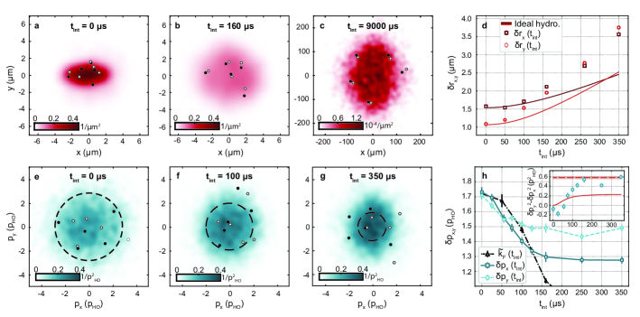
Figure 1: Hydrodynamic expansion. We prepare 5+5 strongly interacting spin up and down atoms (black/white dots) in the ground state of an elliptically shaped trap. We measure their positions (a-c) or momenta (e-g). The two dimensional histograms show the density distribution, obtained from averaging over many experimental realizations of the same quantum state. The initial system has an elliptic density distribution in real space and a round Fermi surface in momentum space (see a and e). We study the expansion after switching off the trap (b-c, f-g) and observe the inversion of the inital aspect ratio in real space and the build up of momentum anisotropy. The dashed black circle in e-g shows the Fermi momentum calculated from the real space peak density. d Root mean square of the atom positions $\delta r_{\text{x}},\delta r_{\text{y}}$ as a function of $t_{\text{int}}$. The expectation assuming ideal hydrodynamic evolution of the corresponding many-body system with the same initial density is shown as a reference (red lines). h Root mean square value $\delta p_{\text{x}},\delta p_{\text{y}}$ of the momenta of the atoms as a function of $t_{\text{int}}$. The triangles show the Fermi momentum $\tilde{k}_{\text{F}}$, rescaled to the geometric mean of $\delta p_{\text{x}},\delta p_{\text{y}}$ at initial time $t_{\text{int}}=$0\text{\,}\mathrm{\SIUnitSymbolMicro}\mathrm{s}$$. The connecting lines serve as a guide to the eye. In the inset, the difference of $\delta p^{2}_{\text{x}}$ and $\delta p^{2}_{\text{y}}$ shows the build up of momentum anisotropy during the interacting expansion. The ideal hydrodynamic expansion (red line) and the asymptotic long term limit derived from the real space data (red dashed line) provide a reference. The error bars of the long term limit are shown by the shaded region. All error bars show the $95\text{\,}\mathrm{\char 37\relax}$ confidence interval, determined using a bootstrapping technique.

Experimental system and observables

We work with a mesoscopic system of ultracold fermionic ⁶Li atoms in the ground state of a potential created by two optical traps. The first one confines the atoms strongly in the vertical direction, creating an effectively two-dimensional (2D) system. The second trap (OT) confines the atoms in the horizontal plane, in an anisotropic, effectively harmonic confinement with trap frequencies $(\omega_{\text{x}},\omega_{\text{y}})/(2\pi)=($1280(3)$,$3384(7)$)\unit{Hz}$ (see Methods). We prepare a discrete many-body quantum state, composed of N spin up and N spin down atoms (denoted N+N) in the ground state, utilizing a technique developed in previous works Serwane_2011 ; Bayha_2020 .

The typical length scales of our system are on the order of the harmonic oscillator length, which is given by $l^{\text{x,y}}_{\text{HO}}=\sqrt{\hbar/m\omega_{\text{x,y}}}\approx($1.1$,$0.7$)\unit{\micro m}$, where $m$ is the mass of a ⁶Li atom. We estimate the typical interparticle spacing from the peak density $n_{0}=(k_{\text{F}}^{0})^{2}/(4\pi)$ of the non-interacting system, with the Fermi wave vector defined as $k^{\text{0}}_{\text{F}}=\sqrt{2mE_{\text{F}}}/\hbar$. Here $E_{\text{F}}$ is the Fermi energy of the non-interacting system, determined by the highest filled energy level of the OT (see Methods). The mean interparticle spacing is $1/\sqrt{n_{0}}\approx$1.3\text{\,}\mathrm{\SIUnitSymbolMicro}\mathrm{m}$$. These length scales are estimated for the non-interacting system, but are on the same order of magnitude in the interacting case. The unitary limit constrains the minimum mean free path to be on the order of the interparticle spacing.

The strength of the attractive interactions can be tuned using the magnetic Feshbach resonance Zuern_2013 . It is quantified by the dimensionless interaction parameter $\text{ln}(k^{\text{0}}_{\text{F}}a_{\text{2D}})$, that relates the initial interparticle spacing (proportional to the inverse of the Fermi wave vector $k^{\text{0}}_{\text{F}}$) to the 2D scattering length $a_{\text{2D}}$ Shlyapnikov2001 ; Materials .

After preparing the system, we remove the horizontal confinement, while keeping the vertical 2D confinement. We let the atoms expand for an interacting expansion time $t_{\text{int}}$. At $t_{\text{int}}$, we instantaneously switch off interactions by a two-photon Raman transition Holten_2022 . Subsequently, we apply matterwave magnification techniques, to image either the momenta Holten_2022 or the positions Subramanian_2023 of the atoms at $t_{\text{int}}$. For the longest interacting expansion time ($t_{\text{int}}=$9\text{\,}\mathrm{m}\mathrm{s}$$), the system has expanded enough for the atoms to be resolvable without matterwave magnification.

We make use of a fluorescence imaging scheme to obtain single atom and spin resolved images Bergschneider_2018 . Each image represents a projection of the wave function on $N+N$ positions or momenta. We obtain the 2D density from approximately 1000 images for each setting (see Methods).

To quantify the widths of the 2D densities, we calculate the root mean square (rms) $\delta$ of the momenta $p$ and positions $r$ over all atoms and images. The rms width in real space is given in $\unit{\micro m}$. We express the momentum rms width $\delta p$ in units of the harmonic oscillator momentum $p_{\text{HO}}=\sqrt{\hbar m\omega_{x}}$ of the weakly confined $x$-direction, to relate to the initial momentum distribution in the trap.

Observing elliptic flow

We investigate the evolution of the 2D density profiles in real and momentum space for a system of $5+5$ atoms and initial interaction parameter $\text{ln}(k^{0}_{\text{F}}a_{\text{2D}})=$1.15$$. The obtained density profiles, superimposed with a randomly chosen single image of both spin states (black and white points), are shown in Fig. 1a-c (real space) and Fig. 1e-g (momentum space).

In real space (see Fig. 1a-d), the system starts from an elliptical density distribution with $\delta r_{\text{x}}>\delta r_{\text{y}}$ and expands anisotropically, with a stronger acceleration along the initially tightly confined direction. After $t_{\text{int}}\gtrsim$250\text{\,}\mathrm{\SIUnitSymbolMicro}\mathrm{s}$$, one observes the characteristic inversion of the initial aspect ratio. Note that after long interacting expansion times we observe molecules (see Fig. 1c).

In order to rule out single particle dynamics stemming from the Heisenberg uncertainty principle, we additionally measure the evolution of the momentum distribution (see Fig. 1e-h). In contrast to the one-body case, the system is initially isotropic, as expected in the many-body limit of a degenerate Fermi gas Pitaevskii_2016 . During the expansion, we observe two main effects in momentum space: the width in both directions decrease and an anisotropy builds up. Both processes subside at $t_{\text{int}}\approx$160\text{\,}\mathrm{\SIUnitSymbolMicro}\mathrm{s}$$.

The increase of anisotropy arises from a redistribution of momenta driven by interactions. This observation is reminiscent of the dynamics of fluids and the unitary Fermi gas Schafer:2009zjw , which exhibit a fast redistribution of momenta followed by the inversion of the initial aspect ratio. Therefore, we interpret our result as the signature of an emergent dynamics driven by a pressure-gradient-type force.

The initial width of the momentum distribution is determined by the Fermi momentum $k_{\text{F}}=\sqrt{4\pi n}$ (see Fig. 1e dashed circle), obtained from the peak real space density $n(t_{\text{int}})=N/(2\pi\delta r_{\text{x}}\delta r_{\text{y}})$. To compare the Fermi momentum to the momentum space rms widths $\delta p_{\text{x,y}}$, we rescale $k_{\text{F}}$ to the geometric mean of $\delta p_{\text{x}}$ and $\delta p_{\text{y}}$ at the initial time $t_{\text{int}}=$0\text{\,}\mathrm{\SIUnitSymbolMicro}\mathrm{s}$$ (denoted $\tilde{k}_{\text{F}}$, shown in Fig 1h). As the system expands in real space the density drops and the Fermi momentum decreases accordingly (see Fig. 1e-g dashed circle and Fig. 1h). For short interacting expansion times, $t_{\text{int}}\lesssim$160\text{\,}\mathrm{\SIUnitSymbolMicro}\mathrm{s}$$, the rescaled Fermi momentum $\tilde{k}_{\text{F}}$ remains comparable to $\delta p_{\text{x,y}}$. For longer times, $\tilde{k}_{\text{F}}$ is smaller than both momentum space widths. The Fermi momentum is comparable to $\delta p_{\text{x,y}}$ up to the time where the redistribution of momenta subsides, indicating that the hydrodynamic description holds only for an interacting degenerate Fermi gas.

The momentum distribution includes both the momentum uncertainty and the velocity field of the system. The framework of hydrodynamics, however contains only the velocity field. It is possible to link the fluid density and velocity to the experimentally observed difference in momentum widths,

$$\frac{m}{2N}\int_{\bf x}\rho(t,\mathbf{x})\left[v_{y}^{2}(t,\mathbf{x})-v_{x}^{2}(t,\mathbf{x})\right]=(\delta p_{y})^{2}-(\delta p_{x})^{2}\,.$$ (1)

This is achieved by relating the momentum flux in the fluid description (interacting atoms) to the one of freely streaming particles (non-interacting atoms) (see Methods). The difference in the squared momenta is shown in the inset of Fig. 1h. This relation allows us to determine the asymptotic limit of the squared momentum differences from the real space data.

In order to understand to which degree the system behaves like a macroscopic fluid, we compare the experimental results to theoretical calculations (see Methods) performed within the framework of ideal hydrodynamics Landau_1987 , i.e. in absence of dissipation. The measured real space density at $t_{\text{int}}=$0\text{\,}\mathrm{\SIUnitSymbolMicro}\mathrm{s}$$ (Fig. 1a) is used as an initial condition for the ideal hydrodynamic expansion, which is simulated by solving the continuity and Euler equation. The pressure as a function of density is required as an additional input for the calculations. It is obtained from the equation of state (EOS) of the corresponding many-body system at low temperature, as determined in experiments on two-dimensional macroscopic Fermi gases 2014PhRvL.112d5301M . The comparison between the simulated real space evolution and the experimental data is shown in Fig. 1d. We extract the difference in velocity fields from the simulation and compare it to the difference in the momentum widths, see inset Fig 1h.

We observe a discrepancy between the experimental results and the theoretical calculations. The pressure used in the simulation would have to be increased approximately two-fold compared to the EOS to find agreement with the experimental data. Finite-size effects, that arise for example, from the single particle gap in our initial, trapped system Bayha_2020 ; Bjerlin_2016 , lead to an increase of the pressure. This is equivalent to the Thomas-Fermi approximation not being valid in our small system Pitaevskii_2016 .

A more accurate description can be achieved by going beyond the Thomas-Fermi approximation. This includes taking into account contributions from local density gradients, known as the von-Weizsäcker term Weizsaecker_1935 ; Salasnich_2013 . Generally, it is expected that higher orders in gradients become more important for small systems.

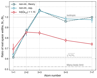
Figure 2: Emergence of hydrodynamics with increasing atom number. The anisotropy of the real space density after an expansion time of $9\text{\,}\mathrm{m}\mathrm{s}$ is quantified by the ratio of the real space rms widths in $x$ and $y$ direction. The non-interacting system (blue dots experimental data, blue squares analytical calculation) evolves from the one-body limit, i.e. the inverse anisotropy of the harmonic oscillator ($\sqrt{\omega_{x}/\omega_{y}}$, dashed line) to the many-body limit, where we observe the build up of an isotropic (dotted line) Fermi surface. The strongly interacting system, characterized by $\text{ln}(k^{0}_{\text{F}}a_{\text{2D}})=1.15$ (red dots), starts from the same one-body limit. For the interacting system, we observe an inversion of the aspect ratio at all atom numbers, with a stronger deviation from the non-interacting system at higher atom numbers. The dashed dotted line shows the numerically calculated final aspect ratio in the many-body limit. The connecting lines serve as a guide to the eye. All error bars show the $95\text{\,}\mathrm{\char 37\relax}$ confidence interval, determined using a bootstrapping technique.

Building a fluid atom by atom

To explore the hydrodynamic behaviour in the few body limit, we study the emergence of elliptic flow for increasing particle numbers starting from a one-body system Floerchinger:2022qem . The dependency of the aspect ratio $\delta r_{\text{x}}/\delta r_{\text{y}}$ after a long expansion time on the atom number is displayed in Fig 2. We compare a strongly interacting system ($\text{ln}(k^{0}_{\text{F}}a_{\text{2D}})=1.15$, red points) to the non-interacting system ($\text{ln}(k^{0}_{\text{F}}a_{\text{2D}})\rightarrow\infty$, blue points) after an expansion time of $9\text{\,}\mathrm{m}\mathrm{s}$.

First, we investigate the non-interacting case. After a non-interacting expansion the final positions are determined by the initial momenta. In the non-interacting system of 1+1 atoms, we observe an inversion of the initial real space aspect ratio ($\delta r_{\text{x}}($0\text{\,}\mathrm{m}\mathrm{s}$)/\delta r_{\text{y}}($0\text{\,}\mathrm{m}\mathrm{s}$)>1$). The momentum space profile of 1+1 non-interacting atoms corresponds to that of a single atom in a harmonic oscillator. A single atom in the ground state has a momentum anisotropy given by the inverse anisotropy of the harmonic oscillator ($\sqrt{\omega_{x}/\omega_{y}})$, which causes the inversion. For larger atom numbers, the non-interacting system becomes increasingly symmetric ($\delta r_{\text{x}}($9\text{\,}\mathrm{m}\mathrm{s}$)/\delta r_{\text{y}}($9\text{\,}\mathrm{m}\mathrm{s}$)=1$), as a round Fermi surface emerges in momentum space. The measured aspect ratio agrees well with the analytical solution of the anisotropic harmonic oscillator ground state (see Methods).

In the case of strongly interacting atoms $(\text{ln}(k^{0}_{\text{F}}a_{\text{2D}})=1.15)$ we see an inversion of the initial aspect ratio for all atom numbers. While there is no significant deviation from the non-interacting case for 1+1 and 2+2 atoms, we observe a strong deviation at higher atom numbers, starting from 3+3 atoms. The final aspect ratio reduces further for increasing atom numbers indicating the emergence of collective behaviour.

In the many-body limit, the local density approximation is applicable and the initial density distribution is described by the Thomas-Fermi (TF) approximation Stringari_2008 , whereby the spatial dependence of the chemical potential becomes determined by the shape of the confining harmonic potential. In the many-body limit, a prediction of $\delta r_{\text{x}}/\delta r_{\text{y}}\rightarrow$0.52$$ can be obtained from solving the hydrodynamic equations using the TF density profile and the pressure determined by the many-body EOS as starting conditions (see Fig. 2) (see Methods).

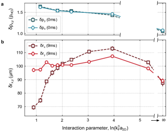
Figure 3: Emergence of hydrodynamics as function of interaction strength. We show the rms widths in momentum $\delta p_{\text{x,y}}($0\text{\,}\mathrm{m}\mathrm{s}$)$ and real space $\delta r_{\text{x,y}}($9\text{\,}\mathrm{m}\mathrm{s}$)$ for different interaction strengths. a The initial momentum distribution remains isotropic for all interaction strenghts, as expected for a degenerate Fermi gas and increases for stronger interactions. b The real space rms widths after $t_{\text{int}}=$9\text{\,}\mathrm{m}\mathrm{s}$$ show the characteristic inversion of the aspect ratio for strong interactions. In the weakly interacting regime, the initial real space anisotropy is preserved. In the non-interacting limit it becomes isotropic, reflecting the initial momentum space profile. The connecting lines serve as a guide to the eye. All error bars show the $95\text{\,}\mathrm{\char 37\relax}$ confidence interval, determined using a bootstrapping technique.

Tuning interactions

In order to investigate the influence of interactions on the expansion, we measure $\delta p_{\text{x,y}}$ at $t_{\text{int}}=$0\text{\,}\mathrm{m}\mathrm{s}$$ and $\delta r_{\text{x,y}}$ after $t_{\text{int}}=$9\text{\,}\mathrm{m}\mathrm{s}$$ for $5+5$ atoms at various interaction strengths. The momentum space data is shown in Fig. 3a, the real space data in Fig. 3b.

As expected for a degenerate Fermi gas, the initial momentum distribution is isotropic ($\delta p_{\text{x}}($0\text{\,}\mathrm{m}\mathrm{s}$)=\delta p_{\text{y}}($0\text{\,}\mathrm{m}\mathrm{s}$)$) for all interaction strengths. Stronger interactions yield a monotonous increase in $\delta p_{\text{x,y}}($0\text{\,}\mathrm{m}\mathrm{s}$)$, as the size of the cloud in real space decreases due to the attractive interactions.

We identify two regimes for the interacting expansion, the strongly ($\text{ln}(k^{0}_{\text{F}}a_{\text{2D}})\lesssim 2$) and the weakly ($\text{ln}(k^{0}_{\text{F}}a_{\text{2D}})\gtrsim 2$) interacting regime . For strong interactions, we observe the emergence of elliptic flow. The final real space distribution becomes increasingly anisotropic with higher interaction strength. Additionally, the rms width along both directions reduces, with a stronger decrease of $\delta r_{\text{x}}$.

In the weakly interacting regime, the final real space widths $\delta r_{\text{x,y}}($9\text{\,}\mathrm{m}\mathrm{s}$)$ do not reflect the shape of the initial momentum profile. Instead, the initial real space anisotropy is conserved ($\delta r_{\text{x}}($0\text{\,}\mathrm{m}\mathrm{s}$)>\delta r_{\text{y}}($0\text{\,}\mathrm{m}\mathrm{s}$))$. This effect decreases with weaker interactions, and is not present in the non-interacting limit $\text{ln}(k^{0}_{\text{F}}a_{\text{2D}})\rightarrow\infty$.

Conclusion and Outlook

We observe elliptic flow – a smoking gun of hydrodynamics – in a mesoscopic quantum gas of ⁶Li atoms. We show that the inversion of the aspect ratio is an interaction driven effect, and that it emerges with increasing atom number. Our measurements challenge the established criteria for a hydrodynamic description since in our experiment, the system size, the interparticle spacing, and the mean free path are not separable.

Our experimental observations might contribute to a deeper understanding of the observed hydrodynamic behaviour in high-energy nuclear collisions in the regime of small particle numbers Nagle:2018nvi ; Schenke:2021mxx . Furthermore, in analogy to the expansion of the quark-gluon plasma (QGP) the transition of our system from strongly interacting to free streaming is accompanied by the formation of bound states – hadrons in the case of QGP and molecules in the case of cold atoms. Our experiment may thus relate to the chemical freeze out of the QGP Andronic:2017pug .

To gain further insight into the mechanism behind the observed hydrodynamic behaviour, we will investigate its connection to the emergence of superfluidity. This has already been seen in helium nanodroplets with tens of atoms Grebenev_1998 . In our system, we can search for signatures of superfluidity by studying the rotational properties, and beyond that exotic strongly correlated quantum states Palm_2020 .

Methods

Preparation Sequence

A detailed description of the preparation scheme can be found in Bayha_2020 . We utilize the same steps to deterministically prepare stable ground state configurations of up to 7+7 atoms in a 2D harmonic oscillator. During the experimental sequence we use the hyperfine states of the ²S${}_{\frac{1}{2}}$ Lithium ground state. The states are labelled in ascending order of energies $\ket{1}-\ket{6}$. First, the ⁶Li atoms are laser cooled by a Zeeman slower and in a magneto optical trap (MOT). From the MOT they are transferred into a red-detuned crossed beam optical dipole trap (CODT), where we utilize a sequence of radio frequency pulses to obtain a balanced mixture of atoms in the hyperfine states $\ket{1}$ and $\ket{3}$.

After evaporating in the CODT, we load the sample in a tightly focused vertical optical tweezer (OT). In the OT we evaporate further and make use of the spilling technique described in Serwane_2011 to end up with a sample of roughly 30 atoms where all states up to the Fermi surface are occupied with high probability.

To prepare the anisotropic 2D sample, we perform a continuous crossover to the quasi-2D regime by ramping up the power of a vertical optical lattice (2D-OT) with trap frequencies of $\omega_{z}/2\pi=$7432(3)\text{\,}\mathrm{H}\mathrm{z}$$ and $\omega^{\text{opt}}_{r}/2\pi=$19.1(1)\text{\,}\mathrm{H}\mathrm{z}$$. Simultaneously we decrease the radial confinement of the OT and adiabatically change its round shape into an elliptic one. The manipulation of the confinement and the shape of the tweezer is controlled by a spatial light modulator in the Fourier plane. Our final trap is an anisotropic 2D harmonic oscillator with trap frequencies of $\omega_{x}/2\pi=$1280(1)\text{\,}\mathrm{H}\mathrm{z}$$, $\omega_{y}/2\pi=$3384(7)\text{\,}\mathrm{H}\mathrm{z}$$ and $\omega_{z}/2\pi=$7432(3)\text{\,}\mathrm{H}\mathrm{z}$$ - see Extended Data Fig. 1.

By using the spilling technique introduced in Bayha_2020 , we prepare the 2D ground state of up to seven atoms per spin state deterministically. The anisotropy of our final trap leads to a different level structure compared to the isotropic harmonic oscillator described in Bayha_2020 (see Extended Data Fig. 1 b,c). With filled harmonic oscillator shells, we can prepare stable ground states of 1+1, 2+2, 3+3, 5+5 and 7+7 atoms with high fidelities.

The interactions are described by the effective 2D scattering length $a_{\text{2D}}$, which is given by Shlyapnikov2001

$$a_{\text{2D}}=\ell_{z}\sqrt{\frac{\pi}{0.905}}\exp(-\ell_{z}/a_{\text{3D}}\sqrt{\pi/2}),$$ (1)

where $\ell_{z}$ is the harmonic oscillator length in the vertical direction and $a_{\text{3D}}$ is the scattering length in a three dimensional (3D) system. The 3D scattering length between two different hyperfine states can be tuned via the magnetic offset field using a Feshbach resonance Zuern_2013 .

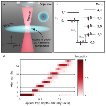
Extended Data Figure 1: Initial system We prepare our initial system in a 2D harmonic oscillator. a The confinement is given by the overlap of a 2D light sheet (2D OT) and a vertical optical tweezer (OT) with elliptical beamshape. b The resulting level scheme of the non-interacting system is characterized by two quantum numbers (n${}_{\text{x}}$, n${}_{\text{y}}$). Shown is a closed shell configuration of 5+5 atoms. The Fermi energy is the energy of the highest occupied level. c By lowering the trap depth, the particles leave the trap shell by shell. Counting the number of atoms as a function of the optical trap depth reveals the level structure of the system. For the weakly-interacting system we find, corresponding to B, filled shells of 1+1, 2+2, 3+3, 5+5 and 7+7 atoms.

Interacting expansion

After preparing the groundstate in the OT, we turn the horizontal confinement off and let the atoms expand in a single plane of the radially symmetric 2D-ODT. We quench off the interactions at a given time $t_{\text{int}}$ after the release from the OT, by driving a Raman transition from the $\ket{1}-\ket{3}$ mixture to the almost non-interacting $\ket{1}-\ket{4}$ mixture. For the $\ket{1}-\ket{4}$ mixture, the scatttering length is equal to that of the singlet with $a_{\text{s}}/a_{\text{0}}=$47(3)$$ Abraham_1996 . The Raman transition is performed on timescales on the order of $300\text{\,}\mathrm{n}\mathrm{s}$. We have previously shown that this timescale is fast enough to preserve correlations in the system Holten_2022 .

In the radial symmetric 2D plane, the radial confinement of the atoms is given by the gaussian optical trap and the harmonic magnetic trap. The optical trap frequency is $\omega^{\text{opt}}_{r}/2\pi=$19.1(1)\text{\,}\mathrm{H}\mathrm{z}$$. The magnetic trap frequency depends on the magnetic field $B$ (given in G) and is given by $\omega^{\text{mag}}_{r}/2\pi=$12.15\text{\,}\mathrm{H}\mathrm{z}$\cdot\sqrt{\frac{B}{700}}$.

For short interacting expansion times, the effect of the radial external potential is negligible. Compared to a free time of flight, the final position differs by less than $1\,\%$. For long interacting expansion times, the potential becomes relevant (deviation $\approx 25\%$), and also depends on the magnetic field. In the analysis we can account for this by solving the equation of motion in the combined trap numerically.

Matterwave magnification

We utilize matterwave magnification techniques to obtain either the position or the momenta of the atoms after short interacting expansion times of up to $350\text{\,}\mathrm{\SIUnitSymbolMicro}\mathrm{s}$. A detailed description for the momentum space measurements can be found in Holten_2022 and in Subramanian_2023 for real space.

To magnify the wavefunction, we switch off interactions at $t=t_{\text{int}}$. The switch-off of interactions is followed by the magnification of the wavefunction. To extract the momenta of the atoms, we let the atoms evolve for $t_{\text{tof}}=$9\text{\,}\mathrm{m}\mathrm{s}$$ in the potential given by the combination of the 2D OT and the magnetic trap. During this expansion the cloud size increases by a factor of $\approx 50$, allowing us to resolve single atoms. Additionally this allows us to map the final positions of the atoms onto their momenta at $t=t_{\text{int}}$. Holten_2022

To image the positions of the particles at $t=t_{\text{int}}$, we utilize the matterwave magnification scheme described in Asteria_2021 ; Subramanian_2023 . The interaction switch off is followed by an expansion in an optical trap with a trap frequency of $\omega_{\text{exp}}/2\pi=$947\text{\,}\mathrm{H}\mathrm{z}$$ for a quarter period. This maps the initial positions $x(t_{\text{int}})$ onto the momenta after the expansion in the optical trap. This is then followed by the same expansion sequence described for momentum space above. The ratio of trap frequencies allows us to magnify the initial positions by a factor of $\approx 42$. This allows us to resolve individual particles and measure their position after the matterwave magnification, which can be directly mapped back to their position at $t=t_{\text{int}}$ Subramanian_2023 .

Imaging

A detailed description of the imaging technique can be found in Bergschneider_2018 ; Holten_2022 . The imaging protocol depends on whether we apply one of the matterwave magnification techniques.

The exact imaging protocol when using matterwave magnification can be found in Holten_2022 . As discussed above, we utilize the non-interacting $\ket{1}-\ket{4}$ mixture for matterwave magnification. Due to technical reasons, the magnetic field is jumped to $750\text{\,}\mathrm{G}$ after the interaction switch-off. During the non-interacting expansion time, we perform two subsequent Landau Zener passages from $\ket{1}\rightarrow\ket{2}\rightarrow\ket{3}$, as $\ket{3}$ has a closed imaging transition. We then image the atoms in $\ket{3}$. After this first image we perform a Landau Zeener passage from state $\ket{4}\rightarrow\ket{3}$ and again take an image of the atoms in $\ket{3}$. As states $\ket{3}$ and $\ket{4}$ are separated by $1.9\,\text{GHz}$, off resonant scattering is highly suppressed.

For measurements without a matterwave magnification protocol, the atoms remain in the $\ket{1}-\ket{3}$ mixture. As the Landau Zeener passages described above take $\approx$8\text{\,}\mathrm{m}\mathrm{s}$$, it is not possible to shift the atoms in $\ket{1}$ to $\ket{3}$, after taking the first image. The imaging transition for $\ket{1}$ is not closed and there is a finite possibility for the atom to decay into a dark state. For imaging atoms in $\ket{3}$, we achieve imaging fidelities of $\approx 98\%$, while the detection fidelity for atoms in $\ket{1}$ is only $\approx 93\%$. In addition, we observe a significantly higher number of off-resonant scattering events compared to the $\ket{1}$ -$\ket{4}$ mixture, due to the smaller detuning of the imaging frequencies. To circumvent this problem, we first image the atoms in $\ket{3}$. These images are then neither affected by off resonant scattering, nor by the finite possibility to decay into a dark state. The atoms in state $\ket{1}$ are also imaged, but the positions are not utilized for the calculation of the rms width due to the abovementioned limitations.

Non-interacting data

The single-particle wavefunction of the two-dimensional harmonic oscillator is given by

$$\begin{split}\Psi_{n,m}(x,y)=&\frac{1}{\sqrt{2^{n}l^{\text{x}}_{\text{HO}}\pi^{1/2}n!}}\text{e}^{-x^{2}/2{l^{\text{x}}_{\text{HO}}}^{2}}\mathcal{H}_{n}(x/l^{\text{x}}_{\text{HO}})\\ &\frac{1}{\sqrt{2^{m}l^{\text{y}}_{\text{HO}}\pi^{1/2}m!}}\text{e}^{-y^{2}/2{l^{\text{y}}_{\text{HO}}}^{2}}\mathcal{H}_{m}(y/l^{\text{y}}_{\text{HO}}),\end{split}$$ (2)

with the harmonic oscillator length in x-, and y-direction $l^{\text{x}}_{\text{HO}}$ and $l^{\text{y}}_{\text{HO}}$, respectively, and the Hermite polynomials of $n$th order $\mathcal{H}_{\text{n}}$.

Exemplary, we show the experimental data and the theoretical calculation of the 5-particle probability density in Extended Data Fig. 2 and Extended Data Fig. 3.

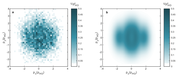
Extended Data Figure 2: Momentum space density of 5+5 non-interacting atoms. Comparison of the experimental and theoretical (a and b, respectively) momentum space density of 5+5 non-interacting atoms in our elliptical trap. The pixel size is given by the pixel size of our camera.

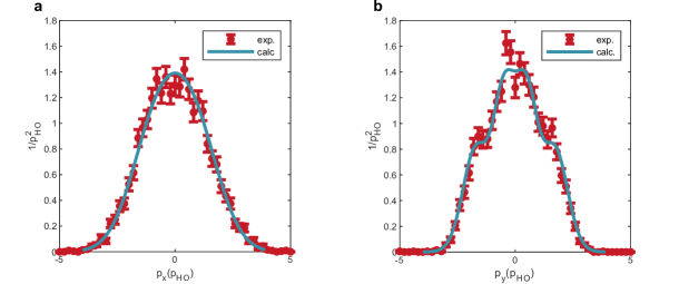
Extended Data Figure 3: Integrated momentum space density of 5+5 non-interacting atoms. The measured and the calculated momentum density gets integrated along y- and x-direction (a and b, respectively). In the errors, the theoretical curve coincides with the experimental curves, showing that the non-interacting system is in the ground state of the harmonic oscillator potential.

Hydrodynamic simulations

The first step in the hydrodynamic modeling is the construction of the initial condition for the expansion, i.e., the mass density, $\rho$, at $t_{\rm int}=0$. As we lack theoretical guidance for the density of a strongly-interacting mesoscopic system, we fit to the measured histogram of atom positions a parametrized function able to match the experimental data. This is achieved with a Fermi-Dirac-type function (where ${\bf x}$ is a coordinate in the $(x,y)$ plane):

$$\rho({\bf x},t_{\rm int}=0)\propto$$

$$\left[1+\exp\left(\frac{(x^{2})^{a_{x}}-b_{x}}{c_{x}}\right)\right]^{-dx}\left[1+\exp\left(\frac{(y^{2})^{a_{y}}-b_{y}}{c_{y}}\right)\right]^{-dy}.$$ (3)

This function is fitted to the histogram of $x$ and $y$ atom positions at $t_{\rm int}=0$, and we have checked that further generalizations through the addition of more parameters do not lead to an improved fit. The mass density is normalized to satisfy:

$$\int d^{2}{\bf x}~{}\rho({\bf x},t_{\rm int})=2mN,$$ (4)

where $m$ is the lithium mass. For the density shown in Fig. 1A, with $N=5$, the fit parameters in Eq. (Hydrodynamic simulations) are $a_{x}=$0.557$$, $b_{x}=$3.155\text{\,}\mathrm{\SIUnitSymbolMicro}\mathrm{m}$$, $c_{x}=$0.904\text{\,}\mathrm{\SIUnitSymbolMicro}\mathrm{m}$$, $d_{x}=$2.171$$, and $a_{y}=$0.173$$, $b_{y}=$0.928\text{\,}\mathrm{\SIUnitSymbolMicro}\mathrm{m}$$, $c_{y}=$0.119\text{\,}\mathrm{\SIUnitSymbolMicro}\mathrm{m}$$, $d_{y}=$0.882$$. Standard errors on these values are of the same order as their absolute magnitudes, as expected from the overfitting of the experimental data.

This initial density profile is then evolved in time according to ideal hydrodynamics. This amounts to solving equations for the conservation of mass, i.e., the fact that integral in Eq. (4) is constant as a function of time, and the conservation of momentum Landau_1987 , respectively,

$$\begin{split}\partial_{t}\rho+\nabla\cdot(\rho{\bf v})&=0\,,\\ \rho(\partial_{t}+{\bf v}\cdot\nabla){\bf v}&=-\nabla P\,,\end{split}$$ (5)

where ${\bf v}=(v_{x},v_{y})$ is the fluid velocity vector. This set of equations is closed by use of a thermodynamic equation of state that relates pressure, $P$, and density. To obtain the pressure, we match our system to the appropriate many-body limit of an interacting Fermi gas at zero temperature in two dimensions. The variation of $P$ as a function of the interaction strength parameter, $\eta=\ln(k_{F}a_{2D})$, is quantified as a deviation from the pressure of the ideal Fermi gas Levinsen2015

$$P_{\rm ideal}\equiv P(\eta\rightarrow\infty)=\frac{\pi\hbar^{2}}{2m^{3}}\rho^{2}.$$ (6)

In the range of $\eta$ relevant to our experimental setup, roughly $\eta<1.2$, an exponential correction to the ideal gas pressure accurately captures the result for $P(\eta)$ obtained from experimental measurements in equilibrium two-dimensional Fermi gases at low temperature 2014PhRvL.112d5301M . From the fit of the experimental data in the region of interest, $-1.7<\eta<1.2$, we obtain the correction

$$P(\eta)=\alpha e^{\beta\eta}P_{\rm ideal},$$ (7)

with $\alpha=$0.216(8)$$ and $\beta=$0.67(5)$$. This allows us to stick to a polytropic-type EOS,

$$P\propto\rho^{2+\beta/2}.$$ (8)

Full solutions of the hydrodynamic equations are finally obtained by means of the compressible hydrodynamic solver of the pyro simulation framework pyro . We compare to experimental data the temporal dependence of the dispersion of the system in real space,

$$\langle\delta r_{x}^{2}\rangle(t_{\rm int})=\frac{\int d^{2}{\bf x}~{}\rho({\bf x},t_{\rm int})x^{2}}{\int d^{2}{\bf x}~{}\rho({\bf x},t_{\rm int})},$$ (9)

and analogously for $\langle\delta r_{y}^{2}\rangle(t_{\rm int})$.

Momentum space analysis

Hereafter we denote by $v_{j}$ the component of the velocity vector ${\bf v}$, where $j$ is either $x$ or $y$. In the conservation law for mass in Eq. (5) the quantity $\mathscr{P}_{j}=\rho v_{j}$ corresponds to the mass current, or flux density, which defines the fluid velocity. In a nonrelativistic system, the mass current corresponds also to the momentum density. Hence, the local momentum conservation law is $\partial_{t}\mathscr{P}_{k}+\partial_{j}\mathscr{P}_{jk}=0$, where the symmetric tensor $\mathscr{P}_{jk}$ is the momentum flux density, with the subscript $k$ also labeling either $x$ or $y$. Fluid dynamics is based on an expansion around local thermal equilibrium in terms of gradients of the fields that characterize equilibrium states. The leading order truncation corresponds to ideal hydrodynamics, for which we have

$$\mathscr{P}_{jk}(t,\mathbf{x})=\rho(t,\mathbf{x})v_{j}(t,\mathbf{x})v_{k}(t,\mathbf{x})+P(t,\mathbf{x})\delta_{jk},$$ (10)

where $P$ is the pressure and $\delta_{jk}$ is the Kronecker symbol.

Experimentally, particle momenta are determined following an instantaneous switch-off of interactions. In a kinetic description, the momentum flux density of a non-interacting system with a phase space distribution $f(t,\mathbf{x},\mathbf{p})=dN/d^{2}xd^{2}p$ involves moments of the momentum distribution,

$$\mathscr{P}_{jk}(t,\mathbf{x})=\int d^{2}p\left\{\frac{p_{j}p_{k}}{m}f(t,\mathbf{x},\mathbf{p})\right\}.$$ (11)

The question is now whether the sudden change in interaction strength enables us to connect the interacting system to the non-interacting one by matching Eq. (10) and Eq. (11) at $t_{\rm int}$.

The instantaneous interaction switch-off is not expected to change $\rho$ or v because they are defined through conserved quantities, but it is expected to change the pressure term, $P$. In the simplest scenario, it would change from the pressure associated with the density in the interacting equation of state, to the one associated with a non-interacting equation of state, though non-equilibrium corrections beyond that should also be expected. To avoid assumptions about the dynamics of the isotropic pressure term, one can thus eliminate such a contribution by studying the difference in Eq. (1). This leads to a solid prediction of the hydrodynamic framework for quantities defined in momentum space.

As discussed in the context of high-energy nuclear collisions Bhalerao:2005mm , the build-up of momentum in a fluid occurs approximately over a time scale $\tau=R/c_{s}$, where $R$ is the system size and $c_{s}$ is the speed of sound. In our case the system size is $R\sim$1\text{\,}\mathrm{\SIUnitSymbolMicro}\mathrm{m}$$, while from the many-body EOS the speed of sound at the center of the cloud is of order $c_{s}=\sqrt{dP/d\rho}\sim$10\text{\,}\mathrm{\SIUnitSymbolMicro}\mathrm{m}\mathrm{/}\mathrm{m}\mathrm{s}$$. Consequently, from a hydrodynamic viewpoint the time scale of the build-up of momentum anisotropy in our system is of order $\tau\sim$0.1\text{\,}\mathrm{m}\mathrm{s}$$. This is consistent with the trends shown in Fig. 1H.

Thomas-Fermi model

From a given equation of state one can obtain a hydrostatic solution in a trap. This is equivalent to the Thomas-Fermi approximation, where the chemical potential is replaced by the space-dependent quantity

$$\mu(x)=\mu_{0}-V(x)\,,$$ (12)

wherever the density is non-vanishing. At constant (in our case zero) temperature we can recover from this and the equation of state $P(\rho)$ the density profile $\rho(x)$ by making use of $\differential{P}=n\differential{\mu}$. This holds as long as there are no relevant derivative corrections through finite size effects. Here we observe deviations of the initial particle density from the Thomas-Fermi prediction that can hence be interpreted as a sign that finite size corrections play an important role in our system. Performing hydrodynamic simulations with the fitted many-body EOS of Eq. (7) and starting with Thomas-Fermi profiles matched to different particle numbers, we find that the baseline aspect ratio at $t_{\rm int}=$9\text{\,}\mathrm{m}\mathrm{s}$$ shown in Fig. 2 is independent of $N$. The origin of this finding as well as corrections to the Thomas-Fermi profile arising from the von-Weizsäcker term Weizsaecker_1935 will be addressed in a separate study.

Data availability

The data that support the findings of this study are available from the corresponding authors upon reasonable request. Source data are provided with this paper.

Acknowledgments

We gratefully acknowledge insightful discussions with Tilman Enss, Aleksas Mazeliauskas, and Jean-Yves Ollitrault. This work has been supported by the Heidelberg Center for Quantum Dynamics, the DFG Collaborative Research Centre SFB 1225 (ISOQUANT), the DFG project DFG FL 736/3-1 (NEQFluids), the Germany’s Excellence Strategy EXC2181/1-390900948 (Heidelberg Excellence Cluster STRUCTURES) and the European Union’s Horizon 2020 research and innovation program under grant agreements No. 817482 (PASQuanS) and No. 725636 (ERC QuStA). This work has been partially financed by the Baden-Württemberg Stiftung.

Author Contributions

S.B. and P.L. contributed equally to this work. S.B., P.L, C.H. and S.J conceived the experiment. S.B. and C.H. performed the measurements. P.L., S.B., and C.H.  analyzed the data. S.J. supervised the experimental part of the project. S.F., G.G., and L.H.H. set up and ran the hydrodynamic simulations. S.B. and P.L. wrote the manuscript with input from all authors. All authors contributed to the discussion of the results.

Competing Interest

The authors declare no competing interests.

Correspondence and requests for materials

should be addressed to S.B. (brandstetter@physi.uni-heidelberg.de) and P.L. (lunt@physi.uni-heidelberg.de)

References

- (1) Mottelson, B. Elementary modes of excitation in the nucleus. (1976). URL https://www.semanticscholar.org/paper/fdf0bf13f2d26cc1ee0101c2250113f7f6f31b20.
- (2) Vogelsberger, M. et al. Properties of galaxies reproduced by a hydrodynamic simulation. Nature 509, 177–182 (2014). URL https://doi.org/10.1038/nature13316.
- (3) Landau, L. & Lifshitz, E. Fluid mechanics (Pergamon Press, 1987).
- (4) Khachatryan, V. et al. Observation of Long-Range Near-Side Angular Correlations in Proton-Proton Collisions at the LHC. JHEP 09, 091 (2010). eprint 1009.4122.
- (5) Abelev, B. et al. Long-range angular correlations on the near and away side in -Pb collisions at TeV. Phys. Lett. B 719, 29–41 (2013). eprint 1212.2001.
- (6) Aad, G. et al. Observation of Associated Near-Side and Away-Side Long-Range Correlations in =5.02 TeV Proton-Lead Collisions with the ATLAS Detector. Phys. Rev. Lett. 110, 182302 (2013). eprint 1212.5198.
- (7) Aidala, C. et al. Creation of quark–gluon plasma droplets with three distinct geometries. Nature Phys. 15, 214–220 (2019). eprint 1805.02973.
- (8) Abdulhamid, M. I. et al. Measurements of the Elliptic and Triangular Azimuthal Anisotropies in Central He3+Au, d+Au and p+Au Collisions at sNN=200 GeV. Phys. Rev. Lett. 130, 242301 (2023). eprint 2210.11352.
- (9) Ollitrault, J.-Y. Anisotropy as a signature of transverse collective flow. Phys. Rev. D 46, 229–245 (1992).
- (10) O’Hara, K. M., Hemmer, S. L., Gehm, M. E., Granade, S. R. & Thomas, J. E. Observation of a strongly interacting degenerate fermi gas of atoms. Science 298, 2179–2182 (2002). URL https://www.science.org/doi/abs/10.1126/science.1079107. eprint https://www.science.org/doi/pdf/10.1126/science.1079107.
- (11) Davis, K. B. et al. Bose-einstein condensation in a gas of sodium atoms. Phys. Rev. Lett. 75, 3969–3973 (1995). URL https://link.aps.org/doi/10.1103/PhysRevLett.75.3969.
- (12) Trenkwalder, A. et al. Hydrodynamic expansion of a strongly interacting fermi-fermi mixture. Phys. Rev. Lett. 106, 115304 (2011). URL https://link.aps.org/doi/10.1103/PhysRevLett.106.115304.
- (13) Fletcher, R. J. et al. Elliptic flow in a strongly interacting normal bose gas. Phys. Rev. A 98, 011601 (2018). URL https://link.aps.org/doi/10.1103/PhysRevA.98.011601. eprint 1803.06338.
- (14) Braun-Munzinger, P. & Stachel, J. The quest for the quark-gluon plasma. Nature 448, 302–309 (2007).
- (15) Busza, W., Rajagopal, K. & van der Schee, W. Heavy Ion Collisions: The Big Picture, and the Big Questions. Ann. Rev. Nucl. Part. Sci. 68, 339–376 (2018). eprint 1802.04801.
- (16) Poskanzer, A. M. & Voloshin, S. A. Methods for analyzing anisotropic flow in relativistic nuclear collisions. Phys. Rev. C 58, 1671–1678 (1998). URL https://link.aps.org/doi/10.1103/PhysRevC.58.1671.
- (17) Bhalerao, R. S., Blaizot, J.-P., Borghini, N. & Ollitrault, J.-Y. Elliptic flow and incomplete equilibration at RHIC. Phys. Lett. B 627, 49–54 (2005). eprint nucl-th/0508009.
- (18) Nagle, J. L. & Zajc, W. A. Small System Collectivity in Relativistic Hadronic and Nuclear Collisions. Ann. Rev. Nucl. Part. Sci. 68, 211–235 (2018). eprint 1801.03477.
- (19) Schenke, B. The smallest fluid on Earth. Rept. Prog. Phys. 84, 082301 (2021). eprint 2102.11189.
- (20) Kurkela, A., Wiedemann, U. A. & Wu, B. Flow in AA and pA as an interplay of fluid-like and non-fluid like excitations. Eur. Phys. J. C 79, 965 (2019). eprint 1905.05139.
- (21) Ambrus, V. E., Schlichting, S. & Werthmann, C. Establishing the Range of Applicability of Hydrodynamics in High-Energy Collisions. Phys. Rev. Lett. 130, 152301 (2023). eprint 2211.14356.
- (22) Serwane, F. et al. Deterministic preparation of a tunable few-fermion system. Science 332, 336–338 (2011).
- (23) Bayha, L. et al. Observing the emergence of a quantum phase transition shell by shell. Nature 587, 583–587 (2020).
- (24) Zürn, G. et al. Precise characterization of Li6 feshbach resonances using trap-sideband-resolved RF spectroscopy of weakly bound molecules. Phys. Rev. Lett. 110, 135301 (2013).
- (25) Petrov, D. S. & Shlyapnikov, G. V. Interatomic collisions in a tightly confined bose gas. Phys. Rev. A 64, 012706 (2001). URL https://link.aps.org/doi/10.1103/PhysRevA.64.012706.
- (26) Materials and methods are available as supplementary materials .
- (27) Holten, M. et al. Observation of cooper pairs in a mesoscopic two-dimensional fermi gas. Nature 606, 287–291 (2022). URL https://doi.org/10.1038/s41586-022-04678-1.
- (28) Subramanian, K. et al. Matterwave magnification of a mesoscopic quantum state of atoms. in preparation (2023).
- (29) Bergschneider, A. et al. Spin-resolved single-atom imaging of Li6 in free space. Phys. Rev. A 97, 063613 (2018).
- (30) Pitaevskii, L. & Stringari, S. Bose-Einstein Condensation and Superfluidity - (Oxford University Press, New York, 2016).
- (31) Schäfer, T. & Chafin, C. Scaling Flows and Dissipation in the Dilute Fermi Gas at Unitarity. Lect. Notes Phys. 836, 375–406 (2012). eprint 0912.4236.
- (32) Makhalov, V., Martiyanov, K. & Turlapov, A. Ground-State Pressure of Quasi-2D Fermi and Bose Gases. Phys. Rev. Lett. 112, 045301 (2014). eprint 1305.4411.
- (33) Bjerlin, J., Reimann, S. & Bruun, G. Few-body precursor of the Higgs mode in a Fermi gas. Phys. Rev. Lett. 116, 155302 (2016).
- (34) v. Weizsaecker, C. F. Zur theorie der kernmassen. Zeitschrift fuer Physik 96, 431–458 (1935). URL https://doi.org/10.1007/bf01337700.
- (35) Salasnich, L., Comaron, P., Zambon, M. & Toigo, F. Collective modes in the anisotropic unitary fermi gas and the inclusion of a backflow term. Phys. Rev. A 88, 033610 (2013). URL https://link.aps.org/doi/10.1103/PhysRevA.88.033610.
- (36) Floerchinger, S., Giacalone, G., Heyen, L. H. & Tharwat, L. Qualifying collective behavior in expanding ultracold gases as a function of particle number. Phys. Rev. C 105, 044908 (2022).
- (37) Giorgini, S., Pitaevskii, L. P. & Stringari, S. Theory of ultracold atomic fermi gases. Rev. Mod. Phys. 80, 1215–1274 (2008). URL https://link.aps.org/doi/10.1103/RevModPhys.80.1215.
- (38) Andronic, A., Braun-Munzinger, P., Redlich, K. & Stachel, J. Decoding the phase structure of QCD via particle production at high energy. Nature 561, 321–330 (2018). eprint 1710.09425.
- (39) Grebenev, S., Toennies, J. P. & Vilesov, A. F. Superfluidity within a small helium-4 cluster: The microscopic andronikashvili experiment. Science 279, 2083–2086 (1998). URL https://www.science.org/doi/abs/10.1126/science.279.5359.2083.
- (40) Palm, L., Grusdt, F. & Preiss, P. M. Skyrmion ground states of rapidly rotating few-fermion systems. New J. Phys. 22, 083037 (2020).
- (41) Abraham, E. R. I. et al. Singlet -wave scattering lengths of and . Phys. Rev. A 53, R3713–R3715 (1996). URL https://link.aps.org/doi/10.1103/PhysRevA.53.R3713.
- (42) Asteria, L., Zahn, H. P., Kosch, M. N., Sengstock, K. & Weitenberg, C. Quantum gas magnifier for sub-lattice-resolved imaging of 3d quantum systems. Nature 599, 571–575 (2021).
- (43) Levinsen, J. & Parish, M. M. Strongly interacting two-dimensional Fermi gases. In Annual Review of Cold Atoms and Molecules - Volume 3. Edited by MADISON KIRK W ET AL. Published by World Scientific Publishing Co. Pte. Ltd, vol. 3, 1–75 (2015). eprint 1408.2737.
- (44) Harpole, A., Zingale, M., Hawke, I. & Chegini, T. pyro: a framework for hydrodynamics explorations and prototyping. Journal of Open Source Software 4, 1265 (2019). URL https://doi.org/10.21105/joss.01265.