GiGaMAE: Generalizable Graph Masked Autoencoder via
Collaborative Latent Space Reconstruction

Abstract.

Self-supervised learning with masked autoencoders has recently gained popularity for its ability to produce effective image or textual representations, which can be applied to various downstream tasks without retraining. However, we observe that the current masked autoencoder models lack good generalization ability on graph data. To tackle this issue, we propose a novel graph masked autoencoder framework called GiGaMAE. Different from existing masked autoencoders that learn node presentations by explicitly reconstructing the original graph components (e.g., features or edges), in this paper, we propose to collaboratively reconstruct informative and integrated latent embeddings. By considering embeddings encompassing graph topology and attribute information as reconstruction targets, our model could capture more generalized and comprehensive knowledge. Furthermore, we introduce a mutual information based reconstruction loss that enables the effective reconstruction of multiple targets. This learning objective allows us to differentiate between the exclusive knowledge learned from a single target and common knowledge shared by multiple targets. We evaluate our method on three downstream tasks with seven datasets as benchmarks. Extensive experiments demonstrate the superiority of GiGaMAE against state-of-the-art baselines. We hope our results will shed light on the design of foundation models on graph-structured data. Our code is available at: https://github.com/sycny/GiGaMAE.

1. Introduction

Figure 1. Preliminary experiments on two downstream tasks (node classification and link prediction) with GraphMAE (Hou et al., 2022) and VGAE (Kipf and Welling, 2016b) on Cora and Computers datasets.

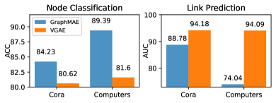
Self-supervised generative models, exemplified by MAE (He et al., 2022) and BERT (Devlin et al., 2018), have demonstrated remarkable performance in acquiring generalizable representations in various domains such as computer vision (Kirillov et al., 2023; Wei et al., 2022) and natural language processing (Zheng et al., 2021). Such representations offer the advantage of being easily adaptable to diverse downstream tasks. In graph domains, generalizable representations also hold significant value in real applications, such as social network platforms where we may want to conduct recommendation (Fan et al., 2019; Tan et al., 2021b, a; Zhou et al., 2021) (link prediction), community detection (Hu et al., 2020b; Tan et al., 2019) (node clustering) and malicious account detection (Cai et al., 2021; Guan et al., 2023; Zhou et al., 2022) (node classification) simultaneously. Thus, generalizable node representations are desirable.

However, we have observed that it is challenging for existing self-supervised generative models on graphs to meet the above expectation. To assess the generalization capacity, we conduct a pilot study on two representative models (VGAE (Kipf and Welling, 2016b) and GraphMAE (Hou et al., 2022)) in Figure 1. We observe that the recently proposed GraphMAE shows good performance in node classification, but it lags behind traditional VGAE in link prediction. Moreover, neither model consistently achieves satisfactory results on both tasks. We have similar observations on other graph generative models as well (e.g., GAE (Kipf and Welling, 2016b), Marginalized GAE (Wang et al., 2017), GATE (Salehi and Davulcu, 2019), and S2GAE (Tan et al., 2023a)), and in other tasks (e.g., node clustering). Based on these observations, we argue that the well-established graph generative methods usually fail to exhibit desirable generalization capabilities across tasks. The limited generalization ability of the model necessitates additional efforts for training on different downstream tasks, which can be time-consuming in practice (Thakoor et al., 2021a).

To understand the generalization issue above, we analyze the state-of-the-art graph generative models and identify the key obstacles. These models typically follow the design of auto-encoding frameworks (He et al., 2022) consisting of an encoder that learns to map the input graph (Hou et al., 2022; Kipf and Welling, 2016b) into latent representations, and a decoder that reconstructs either the observed edges (Kipf and Welling, 2016b) or raw node features (Hou et al., 2022; Wang et al., 2017) from the latent space. Despite their simplicity and popularity, we argue that such a naive reconstruction task is sub-optimal for graph representation learning. This is mainly because graphs are heterogeneous data, containing multiple modalities of information (node features and graph topology). Simply reconstructing a single modality only captures limited aspects of information in the learned representations (Huang et al., 2021). Therefore, a model achieves good performance in a specific downstream task if the corresponding graph information is encoded in embeddings. For example, preserving local information such as node features (e.g., GraphMAE) could benefit node classification, while learning graph structural information results in embeddings that are effective for link prediction or clustering. This motivates us to design a more comprehensive self-supervised reconstruction objective to enhance the generalization ability of representations.

However, this is nontrivial due to the following challenges. (i) Graph reconstruction incompatibility. Graph topology and attributes possess distinct characteristics. Graph edges are discrete and sparse, while node features are continuous and often high-dimensional. This fundamental incompatibility makes it difficult to reconstruct both edges and features simultaneously. Furthermore, previous research has shown that directly reconstructing both edges and features can adversely impact model performance (Hou et al., 2022). (ii) Limitations of existing learning objectives. Current learning objectives are predominantly designed for reconstructing a single modality and do not account for the joint reconstruction of both topology and attribute information. For example, Mean Square Error (MSE) is employed for feature reconstruction tasks, while Binary Cross Entropy (BCE) is used for link prediction tasks. A straightforward approach would be to combine these objectives. However, such optimization goals impose conflicting requirements on the reconstruction model, leading to gradient conflicts (Yu et al., 2020; Lin et al., 2021) and resulting in sub-optimal performance.

In this paper, we propose a novel self-supervised generative model on graphs, called GiGaMAE (Generalizable Graph Masked AutoEncoder), to tackle the above challenges. For challenge (i), instead of directly recovering edges and node features, we map information into a homogeneous latent space for reconstruction. To be more concrete, we use embeddings from multiple external models (e.g., node2vec (Grover and Leskovec, 2016) and PCA (Abdi and Williams, 2010)) as the reconstruction targets. These targets encompass diverse information and can be reconstructed in a unified way, which facilitates the learning of generalizable representation. For challenge (ii), we leverage the Infomax principle (Tschannen et al., 2019) and design a mutual information based reconstruction loss. This loss explicitly captures the shared information between graph topology and node attributes, and distinguishes the distinctive information from different sources. In our framework, we prioritize learning from the shared information since it contains more underlying knowledge, thus enhancing generalization capabilities. We evaluate our framework on various tasks, including node classification, node clustering, and link prediction. The main contributions of this paper are summarized below:

• We investigate how to enhance the generalization capability of self-supervised graph generative models, and propose a novel approach called GiGaMAE by reconstructing graph information in the latent space.

• We propose a novel self-supervised reconstruction loss. This loss effectively characterizes, balances, and integrates both shared and distinct information across multiple collaborative reconstruction targets.

• We conduct extensive experiments on seven benchmark datasets to evaluate the generalization ability of GiGaMAE. Empirical results demonstrate the superiority of our proposed method across three critical graph analysis tasks compared to state-of-the-art baselines.

2. Preliminaries

2.1. Mutual Information (MI)

We resort to mutual information (MI) (Shannon, 1948; Shi et al., 2023b) for the learning objective design in our paper since it can measure the dependency relationship between variables (Tishby et al., 2000; Gabrié et al., 2018).

Mutual Information

The mutual information between two variables $X_{1},X_{2}$ is defined as:

(1) $$\begin{split}&I(X_{1};X_{2})=KL(P_{(X_{1},X_{2})}||P_{X_{1}}P_{X_{2}})\\ =&\sum_{x_{1}\in X_{1}}\sum_{x_{2}\in X_{2}}P_{(X_{1},X_{2})}(x_{1},x_{2})\log\left(\frac{P_{(X_{1},X_{2})}(x_{1},x_{2})}{P_{X_{1}}(x_{1})P_{X_{2}}(x_{2})}\right),\end{split}$$

where $P_{X_{1}}$ and $P_{X_{2}}$ denote the marginal distributions of $X_{1}$ and $X_{2}$, $P_{(X_{1},X_{2})}$ means the joint distribution. $KL(\cdot||\cdot)$ is the Kullback–Leibler divergence (Csiszár, 1975). Multivariate mutual information is a more general definition of dependency measurement if there are more than two variables. The multivariate mutual information between $n\geq 3$ variables $X_{1},X_{2},...,X_{n}$ is defined as below:

(2) $$I(X_{1};...;X_{n})=I(X_{1};...;X_{n-1})-I(X_{1};...;X_{n-1}|X_{n}),$$

where $I(X_{1};...;X_{n-1}|X_{n})$ is the conditional mutual information given the variable $X_{n}$.

Chain Rules for Mutual Information

Specifically, given three random variables $X_{1}$, $X_{2}$, and $X_{3}$, two chain rules for mutual information are listed below:

(3) $$I(X_{1};X_{2},X_{3})=I(X_{1};X_{3})+I(X_{1};X_{2}|X_{3}),$$

(4) $$I(X_{1};X_{2};X_{3})=I(X_{1};X_{2})+I(X_{1};X_{3})-I(X_{1};X_{2},X_{3}).$$

The proof for Equation (3)$\sim$(4) is provided in the Appendix.

Figure 2. The framework of GiGaMAE. Top: The training pipeline. Bottom: We learn different information for nodes with different types of masking. The red shadow region in the Venn Diagram highlights the information to be learned by $\mathbf{S}[i]$.

2.2. Mutual Information Estimation

It is difficult to directly compute MI, because the input distribution is usually unknown. Various methods have been proposed to estimate MI (Poole et al., 2019). In this paper, we select InfoNCE (Oord et al., 2018) as the estimator, which has been empirically proven to be effective in various scenarios (Tschannen et al., 2019; Chen et al., 2020). Given a pair of node representations $(p_{i}$, $q_{i})$ as input, the InfoNCE loss $\ell^{\mathcal{D}}{(p_{i},q_{i})}$ can be defined as:

(5) $$\ell^{\mathcal{D}}{(p_{i},q_{i})}=\log\frac{\mathcal{D}\left(p_{i},q_{i}\right)}{\sum_{i^{\prime}=1}^{N}\mathcal{D}(p_{i},q_{i^{\prime}})+\sum_{i^{\prime}=1}^{N}\mathcal{D}(p_{i},p_{i^{\prime}})-\mathcal{D}(p_{i},p_{i})},$$

where $N$ denotes the number of negative examples, and $\mathcal{D}(\cdot,\cdot)$ denotes the discriminator function. Intuitively, $\mathcal{D}(\cdot,\cdot)$ assigns high values to positive pairs and low values to all other pairs (Veličković et al., 2018; Tschannen et al., 2019). In this paper, we define positive pairs as distinct latent representations of the same node in a graph, whereas negative examples are all the representations of other nodes within the same graph. Then, the overall objective for set $\mathcal{P}$ and $\mathcal{Q}$ (they both contain $N^{\prime}$ node representations) is defined as:

(6) $$\mathcal{L}_{\mathcal{D}}(\mathcal{P},\mathcal{Q})=\frac{1}{2N^{\prime}}\sum_{i=1}^{N^{\prime}}[\ell^{\mathcal{D}}{(p_{i},q_{i})}+\ell^{\mathcal{D}}{(q_{i},p_{i})}],$$

where $p_{i}\in\mathcal{P},q_{i}\in\mathcal{Q}$. The loss $\mathcal{L}_{\mathcal{D}}(\mathcal{P},\mathcal{Q})$ is a lower bound of mutual information $I(\mathcal{P},\mathcal{Q})$ (Poole et al., 2019). Specifically, we can maximize the mutual information by maximizing its corresponding InfoNCE loss.

2.3. Problem Definition

We define a graph as $\mathcal{G}=\left\{\mathcal{V},\textbf{A},\textbf{X}\right\}$, where $\mathcal{V}$ denotes the node set, $\textbf{A}\in\left\{0,1\right\}^{|\mathcal{V}|\times|\mathcal{V}|}$ is the adjacency matrix, and $\textbf{X}\in\mathbb{R}^{|{\mathcal{V}}|\times D}$ is the feature matrix with $D$-dimensional features for each node. Given a graph $\mathcal{G}$ as input, our framework aims to obtain generalizable node representations $\mathbf{Z}\in\mathbb{R}^{|\mathcal{V}|\times d}$, where $d$ is the latent dimension. $\mathbf{z}_{i}=\mathbf{Z}[i,:]$ denotes the representation of node $v_{i}\in\mathcal{V}$.

Problem 1.

Learning Generalizable Graph Representations. Given an input graph $\mathcal{G}$, our goal is to pre-train a generative model to learn node representations $\mathbf{Z}$ that demonstrate consistently competitive performance across commonly studied downstream tasks, including node classification, node clustering, and link prediction.

3. Methodology

We now present GiGaMAE framework. In Section 3.1, we provide an overview of our model as a graph masked autoencoder. In Section 3.2, we introduce the details of the loss function design for training the model. Finally, in Section 3.3, we discuss different candidates as reconstruction targets in the masked autoencoder.

3.1. Framework Design

Our GiGaMAE framework is based on a graph masked autoencoder, as depicted in Figure 2. Unlike previous works that directly reconstruct the original graph information (e.g., node features and graph topology), we employ the output of other graph representation models as the reconstruction targets. The details are given below.

3.1.1. Graph Masked Autoencoder.

A typical graph masked autoencoder consists of three components: a graph augmenter $f^{aug}(\cdot)$, an encoder $f^{enc}(\cdot)$, and a decoder $f^{dec}(\cdot)$. The original graph $\mathcal{G}$ serves as the input and undergoes masking to become $\mathcal{G}^{\prime}=f^{aug}(\mathcal{G})$ through edge masking (Tan et al., 2023a) or feature masking (Wang et al., 2017). The encoder $f^{enc}(\cdot)$ takes $\mathcal{G}^{\prime}$ as input and encodes the nodes into representations $\mathbf{Z}$. Commonly used GNN architectures, such as GAT (Veličković et al., 2017) and GCN (Kipf and Welling, 2016a; Shi et al., 2023a), can be applied for the encoder. Finally, the decoder $f^{dec}(\cdot)$ reconstructs graph components, such as edges or features, from the latent representations $\mathbf{Z}$. The learning objective is typically set as maximizing the accuracy of reconstructing the masked graph components. Graph masked autoencoders have attracted increasing attention recently, but it is challenging for them to produce generalizable representations, due to the limitation in data augmentation and reconstruction objective design. To tackle these issues, we propose a more comprehensive graph augmenter in Section 3.1.2 and an enhanced reconstruction strategy in Section 3.1.3.

3.1.2. Edge and Feature Masking.

Existing graph generative models commonly employ masking over either edges or features of the input graph, while keeping the other modality intact (Hou et al., 2022; Salehi and Davulcu, 2019; Park et al., 2019). Masking both modalities together will negatively affect model learning since it may lack sufficient information for graph reconstruction. However, solely masking and reconstructing one modality limits the model’s ability to learn from the other modality, which hinders the learning of comprehensive representations. In this work, we mask both edges and features of the original graph during training. This results in an augmented graph $\mathcal{G}^{\prime}=f^{aug}(\mathcal{G})=\{\mathcal{V},\textbf{A}^{\prime},\textbf{X}^{\prime}\}$, where $\textbf{A}^{\prime}$ and $\textbf{X}^{\prime}$ denote the masked feature matrix and the masked adjacent matrix, respectively. Formally, we design the augmenter as $f^{aug}(\{\mathcal{V},\textbf{A},\textbf{X}\})=\{\mathcal{V},\textbf{A}\odot\textbf{M}^{\text{E}},\text{diag}(\textbf{M}^{\text{F}})\cdot\textbf{X}\}$, where $\odot$ stands for the Hadamard product. The edge-mask matrix $\textbf{M}^{\text{E}}\in\left\{0,1\right\}^{|\mathcal{V}|\times|\mathcal{V}|}$ and the feature-mask matrix $\textbf{M}^{\text{F}}\in\left\{0,1\right\}^{|\mathcal{V}|}$ are randomly generated binary matrices. The perturbation can be controlled by the sparsity of $\textbf{M}^{\text{E}}$ and $\textbf{M}^{\text{F}}$. After data augmentation, we divide the nodes $\mathcal{V}$ into four types: 1) nodes without any masks $\mathcal{V}^{N}$; 2) nodes with masked edges $\mathcal{V}^{E}$; 3) nodes with masked features $\mathcal{V}^{F}$; and 4) nodes with both masked features and edges $\mathcal{V}^{B}$, where $\mathcal{V}=\mathcal{V}^{N}\cup\mathcal{V}^{E}\cup\mathcal{V}^{F}\cup\mathcal{V}^{B}$. The masked graph is fed into the encoder to obtain the latent representations $\textbf{Z}=f^{enc}(\textbf{A}^{\prime},\textbf{X}^{\prime})$.

3.1.3. Reconstruction Targets.

Different from conventional methods that reconstruct edges or features, we propose to reconstruct the embeddings of other graph models as targets. Here we consider multiple graph models, and $\textbf{Z}_{n}\in\mathbb{R}^{|\mathcal{V}|\times d_{n}}$ denotes the $n$-th reconstruction target. Different graph models focus on learning different graph information. For example, node2vec (Grover and Leskovec, 2016) prioritizes the learning of graph structure information, while PCA (Candès et al., 2011) trained on feature matrix $\mathbf{X}$ mainly encodes node attribute information. The information from various modalities is preserved in continuous embedding spaces $\{\textbf{Z}_{n}\}$ that are homogeneous. By reconstructing these embeddings, we could learn representations that contain both graph topology and attribute information.

Before reconstruction, we further apply re-masking (Hou et al., 2022) on Z to obtain more compressed representations $\textbf{S}\in\mathbb{R}^{|\mathcal{V}|\times d}$. Formally, let $\mathbf{s}_{i}=\textbf{S}[i,:]$ denote the representation of node $v_{i}$:

(7) $$\mathbf{s}_{i}=\begin{cases}f^{enc}(\textbf{A}^{\prime},\textbf{X}^{\prime})[i,:]&\text{ if }v_{i}\in\mathcal{V}^{E}\cup\mathcal{V}^{F}\cup\mathcal{V}^{B}\\ \textbf{0}&\text{ if }v_{i}\in\mathcal{V}^{N}\end{cases},$$

where 0 is a $d$-dimension all-zero vector. Meanwhile, we also apply re-masking on $\mathbf{Z}_{n}$ to obtain $\mathbf{T}_{n}$. Let $\mathbf{t}^{n}_{i}=\textbf{T}_{n}[i,:]$, then $\mathbf{t}^{n}_{i}=\textbf{Z}_{n}[i,:]$ if $v_{i}\notin\mathcal{V}^{N}$, and $\mathbf{t}^{n}_{i}=\textbf{0}\text{ if}\,\,v_{i}\in\mathcal{V}^{N}$. We implement the decoder with a set of projectors $\{f^{proj}_{n}(\cdot)\}$, which map S to the target embedding space $\{\mathbf{T}_{n}\}$. The projected representation is defined as $\textbf{S}_{n}=f^{proj}_{n}(\textbf{S})\in\mathbb{R}^{|\mathcal{V}|\times d_{n}}$. Each projector is implemented as a multi-layer perceptron (MLP).

3.1.4. The Training Objective

Given the compressed representations $\mathbf{S}$ and target embeddings $\mathbf{T}_{1},\mathbf{T}_{2},...,\mathbf{T}_{n}$, the learning objective of our proposed framework is defined as follows:

(8) $$\underset{\theta}{\text{min}}\;\;\mathcal{-L}(\mathbf{S},\{\mathbf{T}_{1},\mathbf{T}_{2},...,\mathbf{T}_{n}\}),$$

where $\theta$ denotes the trainable parameters in our model, including the parameters in $f^{enc}$ and $\{f^{proj}_{n}\}$. The objective encourages $\mathbf{S}$ to preserve the knowledge across different targets, which requires an effective and flexible loss function. Previous research has explored various loss functions, such as the $l_{2}$-norm loss (Salehi and Davulcu, 2019; Park et al., 2019) and the cross-entropy loss (Kipf and Welling, 2016b). However, the $l_{2}$-norm loss considers each feature channel independently and neglects their dependencies, leading to sub-optimal results (Tian et al., 2019). On the other hand, the cross-entropy loss is only applicable to discrete labels. Hence, none of them is suitable for our problem. In the next section, we design a new loss to tackle the challenge.

3.2. Reconstruction Loss Design

We propose a mutual information (MI) based reconstruction loss to effectively learn knowledge from multiple collaborative targets. To facilitate illustration, we first consider the case of a single target and then extend it to handle multiple targets.

3.2.1. Single-Target Reconstruction.

We start by discussing the scenario where we have a single reconstruction target $\mathbf{T}$. Our goal is to optimize the generative model’s representations to capture as much useful information as possible from the target. To achieve this, we define our learning objective as maximizing the MI between $\mathbf{S}$ and $\mathbf{T}$, denoted as $\mathcal{L}_{\text{Single}}=I(\mathbf{S};\mathbf{T})$. According to Equation (6), the objective can be optimized by maximizing the InfoNCE loss (Oord et al., 2018):

(9) $$\hat{\mathcal{L}}_{\text{Single}}=\mathcal{L}_{\mathcal{D}}(\mathbf{S},\mathbf{T}),$$

where $\hat{\mathcal{L}}_{\text{Single}}$ is a lower bound of $I(\mathbf{S};\mathbf{T})$. Specifically, the discriminator $\mathcal{D}$ used in $\mathcal{L}_{\mathcal{D}}$ is formulated following (Veličković et al., 2018; Tian et al., 2020) as:

(10) $$\mathcal{D}(\mathbf{s},\mathbf{t})=\exp\left(\frac{f^{proj}\left(\mathbf{s}\right)\cdot\mathbf{t}}{\left\|f^{proj}\left(\mathbf{s}\right)\right\|\cdot\left\|\mathbf{t}\right\|}\cdot\frac{1}{\tau}\right),$$

where $f^{proj}$ is the projector function, and $\tau$ denotes the temperature hyper-parameter. Intuitively, the information in $\mathbf{t}$ is reconstructed from $\mathbf{s}$ via maximizing the similarity between $\mathbf{t}$ and $f^{proj}(\mathbf{s})$.

3.2.2. Dual-Target Reconstruction.

We then discuss how to extend the single-target scenario to deal with dual targets that could cover heterogeneous modalities. A naive design is to maximize the similarity between the projected representation $\mathbf{S}_{n}$ and the target representation $\mathbf{T}_{n}$. However, this approach learns from each target individually, failing to capture the information shared between them, which could contain crucial common knowledge that the model should emphasize. To overcome this issue, we propose to quantify this shared knowledge using MI. Specifically, we use $I(\mathbf{S};\mathbf{T}_{1};\mathbf{T}_{2})$ to define the common knowledge shared between $\mathbf{T}_{1}$ and $\mathbf{T}_{2}$ learned by $\mathbf{S}$. Meanwhile, we use $I(\mathbf{S};\mathbf{T}_{1}|\mathbf{T}_{2})$ and $I(\mathbf{S};\mathbf{T}_{2}|\mathbf{T}_{1})$ to define the unique knowledge solely from $\mathbf{T}_{1}$ and $\mathbf{T}_{2}$, respectively, that is learned by $\mathbf{S}$. As the two targets could preserve different knowledge, their weights may differ. Hence, we propose to treat each part of knowledge separately by presenting a more general form of Equation (9) as below:

(11) $$\mathcal{L}_{\text{Dual}}=\lambda_{1}I(\mathbf{S};\mathbf{T}_{1}|\mathbf{T}_{2})+\lambda_{2}I(\mathbf{S};\mathbf{T}_{2}|\mathbf{T}_{1})+\lambda_{3}I(\mathbf{S};\mathbf{T}_{1};\mathbf{T}_{2}).$$

The parameters $\lambda_{1}$, $\lambda_{2}$, and $\lambda_{3}$ control the influence of each part of knowledge in model training. A larger value of $\lambda$ indicates a greater importance assigned to the corresponding knowledge. In Equation (11), it is challenging to directly estimate the conditional mutual information or the multivariate mutual information involving three variables with existing methods (Poole et al., 2019). To address this, we employ chain rules to transform the loss function as:

$$\mathcal{L}_{\text{Dual}}= \,\,\lambda_{1}[I(\mathbf{S};\mathbf{T}_{1},\mathbf{T}_{2})-I(\mathbf{S};\mathbf{T}_{2})]+\lambda_{2}[I(\mathbf{S};\mathbf{T}_{1},\mathbf{T}_{2})-I(\mathbf{S};\mathbf{T}_{1})]$$

$$+\lambda_{3}[I(\mathbf{S};\mathbf{T}_{1})+I(\mathbf{S};\mathbf{T}_{2})-I(\mathbf{S};\mathbf{T}_{1},\mathbf{T}_{2})]$$

$$= \,\,(\lambda_{3}-\lambda_{2})\cdot I(\mathbf{S};\mathbf{T}_{1})+(\lambda_{3}-\lambda_{1})\cdot I(\mathbf{S};\mathbf{T}_{2})$$

(12) $$+(\lambda_{1}+\lambda_{2}-\lambda_{3})\cdot I(\mathbf{S};\mathbf{T}_{1},\mathbf{T}_{2}),$$

where the transformed mutual information can be estimated by the InfoNCE loss. Thus, the dual-target reconstruction loss used for model training is defined as:

(13) $$\begin{split}\hat{\mathcal{L}}_{\text{Dual}}&=\tilde{\lambda}_{1}\mathcal{L}_{\mathcal{D}_{1}}(\mathbf{S},\mathbf{T}_{1})+\tilde{\lambda}_{2}\mathcal{L}_{\mathcal{D}_{2}}(\mathbf{S},\mathbf{T}_{2})+\tilde{\lambda}_{3}\mathcal{L}_{\mathcal{D}_{3}}(\mathbf{S},\{\mathbf{T}_{1},\mathbf{T}_{2}\}),\end{split}$$

where $\tilde{\lambda}_{1}=(\lambda_{3}-\lambda_{2})$, $\tilde{\lambda}_{2}=(\lambda_{3}-\lambda_{1})$, $\tilde{\lambda}_{3}=(\lambda_{1}+\lambda_{2}-\lambda_{3})$ are the reorganized weight hyper-parameters. And we set $\tilde{\lambda}_{1},\tilde{\lambda}_{2},\tilde{\lambda}_{3}\geq 0$. $\mathcal{L}_{\mathcal{D}_{1}}$ and $\mathcal{L}_{\mathcal{D}_{2}}$ apply $\mathcal{D}_{1}$ and $\mathcal{D}_{2}$ as their discriminator, which have the same formula as Equation (10) with $f^{proj}_{1}:\mathbb{R}^{|\mathcal{V}|\times d}\rightarrow\mathbb{R}^{|\mathcal{V}|\times d_{1}}$ and $f^{proj}_{2}:\mathbb{R}^{|\mathcal{V}|\times d}\rightarrow\mathbb{R}^{|\mathcal{V}|\times d_{2}}$ as projectors, respectively. $\mathcal{L}_{\mathcal{D}_{3}}$ applies $\mathcal{D}_{3}$ as the discriminator which is applicable given three input variables. We define $\mathcal{D}_{3}$ as:

(14) $$\mathcal{D}_{3}(\mathbf{s},\{\mathbf{t}_{1},\mathbf{t}_{2}\})=\exp\left(\frac{f^{proj}_{3}\left(\mathbf{s}\right)\cdot[\mathbf{t}_{1};\mathbf{t}_{2}]}{\left\|f^{proj}_{3}\left(\mathbf{s}\right)\right\|\cdot\left\|[\mathbf{t}_{1};\mathbf{t}_{2}]\right\|}\cdot\frac{1}{\tau}\right),$$

where $f^{proj}_{3}:\mathbb{R}^{|\mathcal{V}|\times d}\rightarrow\mathbb{R}^{|\mathcal{V}|\times(d_{1}+d_{2})}$ will map the compressed representations to the concatenated dimension, and $[;]$ denotes concatenation. In particular, when $\lambda_{1}=\lambda_{2}$ and $\lambda_{3}=\lambda_{1}+\lambda_{2}$, the knowledge learned from different sources is treated equally.

3.2.3. Multiple-Target Reconstruction.

A general version of loss that handles $n\geq 3$ targets can be derived from the dual-target loss as:

(15) $$\hat{\mathcal{L}}_{\text{Multi}}=\sum_{i\in 2^{n}-1}\tilde{\lambda}_{i}\mathcal{L}_{D_{i}}(\mathbf{S},\{\mathcal{T^{\prime}}\}_{i}),$$

where $\mathcal{T}=\{\mathbf{T}_{1},\mathbf{T}_{2},...,\mathbf{T}_{n}\}$ is the set of target embeddings, and the $\mathcal{T^{\prime}}=\{\mathbf{T}_{1},\mathbf{T}_{2},\mathbf{T}_{3},...,\{\mathbf{T}_{1},\mathbf{T}_{2}\},\{\mathbf{T}_{1},\mathbf{T}_{3}\},...,\{\mathbf{T}_{1},\mathbf{T}_{2},...,\mathbf{T}_{n}\}\}$ is the collective set formed by every subset of $\mathcal{T}$. According to Equation (15), as the number of targets increases, the computational cost will increase rapidly. However, in practice, many graph models produce highly similar embeddings containing overlapping information, so we can remove the overlapping targets without affecting the performance. Our experiment results show that state-of-the-art downstream task performance can be achieved with no more than three targets. This observation is also consistent with current research findings on multi-view learning (Tian et al., 2020; Hassani and Khasahmadi, 2020), where too many targets are not necessarily needed for desirable results.

3.3. Reconstruction Target Candidates

In this subsection, we discuss how to choose reconstruction targets and how to choose their weights.

3.3.1. Reconstruction Target.

A wide range of graph embedding models are potential candidates. We categorize the candidates into three groups based on their input and inductive bias.

Target embeddings with structural knowledge.

This group of target embeddings captures the original graph’s topological or structural information. Examples include Grarep (Ahmed et al., 2013), Deepwalk (Perozzi et al., 2014), and node2vec (Grover and Leskovec, 2016). In this paper, we use the output of node2vec as our structural target embedding. Given a graph $\mathcal{G}=\{\mathcal{V},\textbf{A}\}$ as input, node2vec generates target embedding that preserves path-aware topological information by employing two traversing strategies: breadth-first sampling (BFS) and depth-first sampling (DFS). The combination of the two strategies enables node2vec to learn comprehensive structural information. Compared with the recent self-supervised learning models (e.g., contrastive learning), node2vec is more efficient due to its lower time and space complexity.

Target embeddings with attribute knowledge.

This group of target embeddings encodes attribute information from an input graph. Examples include principal component analysis (PCA) (Candès et al., 2011) and autoencoder (Wang et al., 2016). In this paper, we choose the output of PCA as our attribute target embedding. Given a graph $\mathcal{G}=\{\mathcal{V},\textbf{X}\}$ as input, PCA maps the feature matrix into a lower-dimensional embedding space, which preserves most of the useful information and eliminates the noise (Salmon et al., 2014). Here PCA is also efficient due to its relatively low time and space complexity. In the rest of the paper, we choose node2vec and PCA as default models to provide embeddings as the reconstruction targets, since they are efficient and can encode distinct information modalities.

Target embeddings with hybrid knowledge.

This group leverages GNNs as encoders to capture both topological and feature information. Examples include graph contrastive learning models (Zhu et al., 2020; You et al., 2020; Thakoor et al., 2021b) and graph generative models (Kipf and Welling, 2016b; Salehi and Davulcu, 2019). In this paper, we select the Graph Autoencoder (GAE) as the hybrid knowledge extractor (Kipf and Welling, 2016b). Given a graph $\mathcal{G}=\{\mathcal{V},\textbf{A},\textbf{X}\}$ as input, the GAE learns target embeddings by reconstructing edges of the original graph. However, GAE comes with a higher computational cost, thus we only include it for performance comparison in the ablation study.

3.3.2. Weight Setting Strategy.

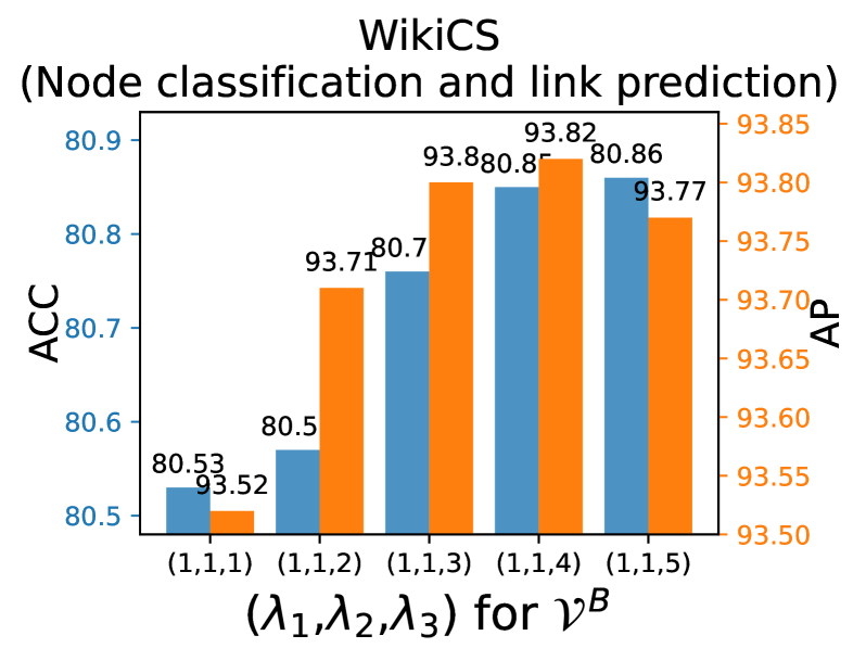
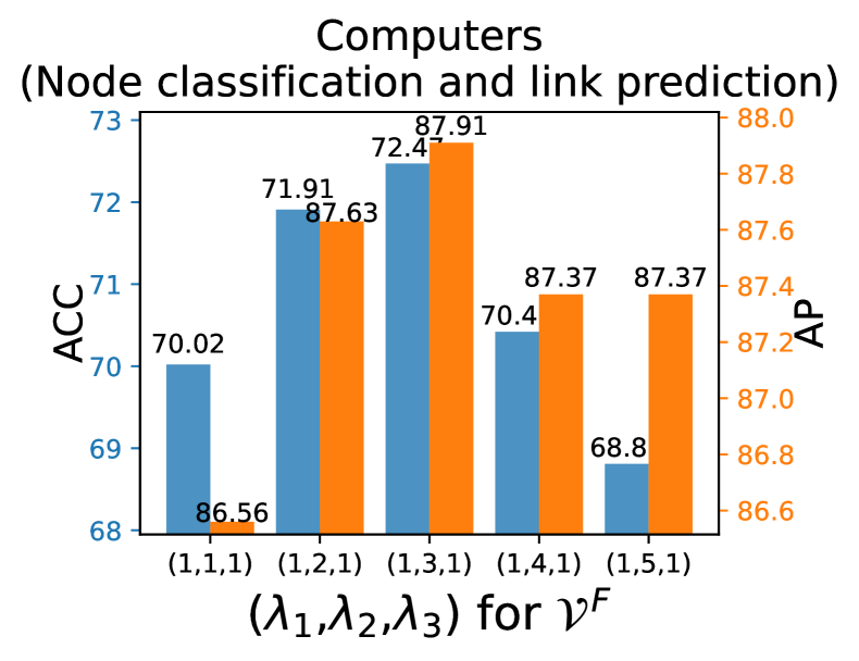
In this paper, we decide the weight value of $\{\lambda_{1},\lambda_{2},...\}$ based on the masking results of $f^{aug}$. The key idea is to prioritize the learning of information that is masked by $f^{aug}$, as shown in Figure 2. For example, suppose we use node2vec as $target_{1}$ and PCA as $target_{2}$. For nodes in $\mathcal{V}^{E}$ whose edges are masked, since $target_{1}$ contains the topological information, we prioritize the learning of this information, meaning that $\lambda_{1}>\lambda_{2}$. In contrast, for nodes in $\mathcal{V}^{F}$, a reasonable setting would be $\lambda_{2}>\lambda_{1}$. In self-supervised learning, this would make the pre-training task more challenging and valuable, encouraging the encoder to learn more generalizable patterns from the input (He et al., 2022; Hou et al., 2022).

Furthermore, $\mathcal{V}^{B}$ consists of nodes with masked edges and features, which results in the absence of both structural and attribute information, making their reconstruction particularly challenging and unstable. To address this, we prioritize the reconstruction of the most fundamental information for nodes in $\mathcal{V}^{B}$. Intuitively, this information refers to the shared knowledge among all target models, which we refer to as common knowledge in Section 3.2.2 and 3.2.3. For example, in the dual-target scenario, a reasonable weight setting for nodes in $\mathcal{V}^{B}$ would be $\lambda_{3}>\lambda_{1}$ and $\lambda_{3}>\lambda_{2}$. We validate the effectiveness of our weight setting strategy through an ablation study in our experiments.

Table 1. Node classification performance comparison (Accuracy). A.R. means the average rank.

Model Type	Dataset	Cora	Citeseer	WikiCS	Computers	Photo	CS	Physics	A.R.
Randwalk	Deepwalk	73.32±0.61	48.24±1.35	76.37±0.19	86.59±0.10	90.08±0.29	85.40±0.13	92.37±0.08	8.86
Contrastive	MVGRL	84.39±0.34	71.71±0.24	80.15±0.27	88.28±0.13	92.29±0.19	92.91 ±0.07	95.36±0.06	4.71
	GCA	83.86±0.45	71.83±0.68	78.86±0.26	88.06±0.12	92.44±0.29	92.66±0.09	95.50±0.18	5.71
	BGRL	82.35±0.26	71.29±0.59	79.47±0.26	89.80±0.17	92.77±0.15	92.60±0.05	95.60±0.04	4.86
Generative	VGAE	80.62±0.32	71.85±1.19	78.21±0.43	81.60±0.28	90.77±0.44	92.41±0.13	95.24±0.03	7.43
	GraphMAE	84.23±0.42	72.74±0.29	80.57±0.17	89.39±0.84	92.83±0.43	92.68±0.30	95.52±0.15	3.29
	GraphMAE2	84.41±0.30	72.11±0.42	81.01±0.34	89.50±0.76	92.87±0.14	92.74±0.14	95.38±0.08	3.00
	S2GAE	84.14±0.65	72.21±0.47	79.14±0.23	89.64±0.12	92.09±0.28	89.92±0.17	94.37±0.14	5.71
Generative	GiGaMAE	84.72±0.47	72.31±0.50	81.14±0.16	90.45±0.16	93.01±0.41	92.72±0.32	95.66±0.14	1.43

Table 2. Node clustering performance comparison (NMI/ARI).

Dataset	Cora	Citeseer	WikiCS	Computers	Photo	CS	Physics	A.R.
Deepwalk	0.4161/0.3416	0.1376/0.1452	0.4660/0.3587	0.4202/0.2637	0.6482/0.5129	0.6445/0.4863	0.6995/0.7985	5.21
MVGRL	0.5481/0.5167	0.4073/0.4115	0.2135/0.1101	0.2657/0.1806	0.1776/0.1127	0.6436/0.4737	0.4948/0.4799	6.79
GCA	0.4645/0.3268	0.2681/0.2178	0.1463/0.0176	0.4062/0.1512	0.4480/0.2518	0.6975/0.5578	0.6638/0.7468	6.93
BGRL	0.2851/0.0920	0.2156/0.1759	0.2767/0.0937	0.4396/0.2096	0.6189/0.4754	0.7740/0.6422	0.7249/0.8130	5.50
VGAE	0.4930/0.4392	0.4104/0.4247	0.3453/0.1478	0.3073/0.2054	0.4847/0.3539	0.7736/0.6646	0.4925/0.2628	5.50
GraphMAE	0.5781/0.5082	0.4330/0.4423	0.4038/0.2951	0.5015/0.3298	0.6676/0.5703	0.7297/0.5691	0.6348/0.6734	3.14
GraphMAE2	0.5821/0.5310	0.4283/0.4268	0.3674/0.2541	0.5053/0.3418	0.6496/0.5613	0.4423/0.2449	0.2820/0.1564	4.50
S2GAE	0.5127/0.4481	0.3346/0.2830	0.3143/0.1110	0.4397/0.2297	0.5624/0.3427	0.6251/0.4289	0.6152/0.7059	5.93
GiGaMAE	0.5836/0.5453	0.4224/0.4283	0.4910/0.4239	0.5228/0.3579	0.7066/0.5859	0.7622/0.6417	0.7373/0.8271	1.50

Table 3. Link prediction performance comparison.

Dataset	Metrics	Cora	Citeseer	WikiCS	Computers	Photo	CS	Physics	A.R.
Deepwalk	AUC	76.33±0.48	64.67±0.61	91.06±0.06	87.36±0.06	91.74±0.09	91.01±0.12	91.94±0.07
	AP	81.77±0.29	72.77±0.49	91.76±0.08	87.34±0.04	91.55±0.08	92.28±0.10	91.93±0.07	6.14
MVGRL	AUC	74.57±0.38	68.33±0.59	93.09±0.14	85.32±0.25	84.89±0.08	77.13±0.33	77.26±0.53
	AP	77.16±0.28	72.79±0.32	93.37±0.15	86.45±0.21	85.54±0.10	78.77±0.35	79.84±0.42	7.64
GCA	AUC	89.88±1.21	87.25±0.87	93.83±0.23	90.95±0.44	91.47±0.47	87.72±0.21	90.45±0.34
	AP	89.39±1.76	87.59±0.65	93.90±0.35	89.80±0.13	91.26±0.46	86.08±0.34	88.12±0.37	5.71
BGRL	AUC	91.70±0.59	92.90±0.57	89.67±0.58	93.69±0.43	94.21±0.64	92.60±0.15	92.29±0.56
	AP	92.18±0.43	93.91±0.44	89.67±0.59	92.86±0.53	93.44±0.65	91.29±0.19	90.79±0.88	4.36
VGAE	AUC	94.18±0.80	93.79±0.21	96.99±0.11	94.09±0.10	95.28±0.14	95.94±0.14	95.88±0.17
	AP	95.12±0.11	93.80±0.23	97.75±0.46	93.84±0.11	94.59±0.16	95.41±0.17	95.24±0.10	2.36
GraphMAE	AUC	88.78±0.87	90.32±1.26	71.40±4.19	74.04±3.08	74.58±3.90	85.37±1.37	81.29±5.13
	AP	88.32±0.91	91.54±0.87	68.60±3.96	70.08±2.80	72.30±3.01	83.93±1.08	79.71±4.40	7.86
GraphMAE2	AUC	89.54±0.30	90.48±0.98	72.71±3.33	73.99±3.04	83.77±1.32	89.22±0.35	83.20±1.43
	AP	88.91±0.31	91.53±0.71	69.66±3.31	70.05±2.76	80.71±1.08	87.13±0.32	82.24±1.05	7.07
S2GAE	AUC	93.12±0.58	93.81±0.23	98.74±0.02	94.59±1.16	93.84±2.22	96.13±0.48	95.21±0.75
	AP	93.96±0.58	94.21±0.24	98.76±0.02	94.01±1.11	92.07±3.12	95.73±0.62	94.56±0.83	2.29
GiGaMAE	AUC	95.13±0.15	94.18±0.36	95.30±0.09	95.17±0.38	96.24±0.11	96.34±0.07	96.32±0.08
	AP	95.20±0.17	94.40±0.12	95.59±0.09	92.91±0.51	94.62±0.11	95.28±0.09	95.27±0.04	1.57

4. Experiments

We conduct experiments to answer the following questions. Q1: Does the proposed method generalize well to the common downstream tasks? Q2: How does our framework perform given different targets with different settings? Q3: Is our reconstruction loss effective with the proposed masking and weight setting strategy?

4.1. Experiments Setup

4.1.1. Datasets and Baselines

We demonstrate the effectiveness of our framework on various node-level tasks. We select seven representative benchmark datasets (Yang et al., 2016; Mernyei and Cangea, 2020; Shchur et al., 2018), including Cora, CiteSeer, WikiCS, Amazon-Computers (Computers), Amazon-Photo (Photo), Coauthor-CS (CS), and Coauthor-Phy (Phy), as benchmarks. Our proposed framework is compared with various types of state-of-the-art models. The first type is contrastive learning models, which include GCA (Zhu et al., 2021), MVGRL (Hassani and Khasahmadi, 2020), and BGRL (Thakoor et al., 2021b). Among them, GCA uses node centrality to generate high-quality contrastive views; MVGRL utilizes multiple views of graphs for contrastive learning; BGRL gets rid of negative examples by leveraging the idea of self-distillation. The second type is generative models, which include VGAE (Kipf and Welling, 2016b), GraphMAE (Hou et al., 2022), GraphMAE2 (Hou et al., 2023), and S2GAE (Tan et al., 2023a). The VGAE and S2GAE aim to predict the existence of edges, and GraphMAE and GraphMAE2 seek to reconstruct the node feature. The last type is a random-walk based model, i.e., Deepwalk (Perozzi et al., 2014).

4.1.2. Experimental Settings

Our proposed framework is implemented in PyTorch (Paszke et al., 2019) and PyG (PyTorch Geometric) (Fey and Lenssen, 2019). The implementation details for baselines and GiGaMAE can be found in the Appendix. Unless otherwise specified, we obtain our target embeddings $\mathbf{T}_{1}$ and $\mathbf{T}_{2}$ using node2vec and PCA, respectively.

Figure 3. The average of A.R. on three tasks (A lower value indicates better performance and generalization ability).

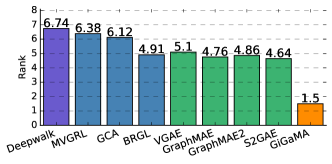
4.2. Quantitative Evaluation

To answer Q1, we benchmark the performance of GiGaMAE on three crucial graph learning tasks: node classification, node clustering, and link prediction. For a clear comparison, we report the average rank (A.R.) along with the corresponding metric scores. We also provide the average value of A.R. on these tasks in Figure 3. We can observe that GiGaMAE is the only method that consistently performs well over the three tasks, which validates its generalization ability. Detailed analysis is as follows.

4.2.1. Node Classification

For the node classification task, we follow the same linear evaluation protocol in (Zhu et al., 2020). First, we use the pre-trained model to generate node representations given the whole graph. Then we evaluate the node representation quality under a logistic-regression classifier using grid-search, where the train/test split follows (Zhu et al., 2020, 2021). It is important to point out that the applied split setting is different from the ones used in (Thakoor et al., 2021b; Hassani and Khasahmadi, 2020; Tan et al., 2023a; Hou et al., 2022, 2023), resulting in slight variations in the reported results. Finally, we report the mean accuracy results with standard deviation on the test nodes for ten runs. The results are listed in Table 1. Our proposed model achieves the best performance in most datasets and ranks top-1 over eight state-of-the-art baselines.

4.2.2. Node Clustering

For the node clustering task, we follow the evaluation protocol in (Park et al., 2019; Wang et al., 2017). The whole data is used in the pre-training process to obtain representations, which are then clustered using the K-Means algorithm with cluster numbers set to label class numbers. We report the mean value of normalized mutual information (NMI) and average rand index (ARI) for ten runs. Table 2 reports the clustering results. Our approach has the best overall clustering performance ranking top-1 against the baselines. We also find that the models (e.g., MVGRL) with good classification performance do not always have good clustering performance, suggesting these two tasks require different kinds of knowledge.

Table 4. Target embeddings performance vs. GiGaMAE performance.

Dataset	Cora			WikiCS			Computers
Metrics	ACC	NMI/ARI	AUC	ACC	NMI/ARI	AUC	ACC	NMI/ARI	AUC
Node2vec	71.76±0.75	0.3944/0.2460	85.85±1.13	71.57±0.36	0.4081/0.3452	91.70±0.26	83.98±0.28	0.5248/0.3882	84.83±0.21
PCA	42.22±0.57	0.0212/0.0068	68.93±0.05	68.52±0.25	0.3181/0.2211	79.03±0.02	66.40±0.25	0.0305/0.0236	59.86±0.02
GAE	81.29±0.61	0.4907/0.4136	90.04±0.15	70.33±0.86	0.1091/0.0603	94.65±0.16	77.01±1.08	0.3204/0.1749	91.58±0.13
GiGaMAENode2vec	84.00±0.51	0.5376/0.4706	93.67±0.19	80.56±0.51	0.4687/0.3592	94.60±0.44	89.98±0.21	0.5089/0.3207	87.71±0.64
GiGaMAEPCA	83.17±0.59	0.5343/0.4861	93.44±0.60	80.96±0.33	0.4810/0.3397	94.59±0.21	90.07±0.16	0.5139/0.3123	89.60±1.97
GiGaMAEGAE	84.14±0.63	0.5802/0.5257	92.78±0.31	80.74±0.30	0.4664/0.3433	94.16±0.13	89.46±0.06	0.5288/0.3843	87.58±0.08
GiGaMAE	84.72±0.47	0.5836/0.5453	95.13±0.15	81.14±0.16	0.4908/0.4211	95.30±0.09	90.45±0.16	0.5228/0.3579	95.17±0.38
GiGaMAELarge	84.69±0.46	0.5808/0.5394	95.12±0.09	81.14±0.20	0.4777/0.3748	95.34±0.04	90.44±0.20	0.5375/0.3901	93.61±0.29

Table 5. Models performance with naive learning objectives and mask strategies.

Dataset		Cora			WikiCS			Computers
Metrics		ACC	NMI/ARI	AUC	ACC	NMI/ARI	AUC	ACC	NMI/ARI	AUC
Naive Integration	MaxPooling	47.24±0.56	0.0621/0.0308	64.05±0.02	57.67±0.38	0.1070/0.0536	60.27±0.02	65.36±0.27	0.0569/0.0067	44.44±0.03
	AvgPooling	58.16±0.88	0.3117/0.2537	72.92±0.03	68.88±0.27	0.1462/0.0661	86.15±0.01	74.20±0.30	0.3414/0.2133	74.87±0.02
	Concatenate	70.94±0.48	0.4119/0.3641	77.59±0.01	74.51±0.30	0.1625/0.0767	89.84±0.01	82.71±0.19	0.3715/0.2218	81.90±0.02
Naive Loss	MSE	83.83±0.70	0.5862/0.5425	56.68±0.13	80.43±0.39	0.4623/0.3639	89.32±0.02	89.85±0.76	0.5182/0.3469	72.75±0.68
	Scaled Cosine	84.10±1.18	0.5489/0.4722	94.22±0.35	80.95±0.20	0.4586/0.3456	91.04±0.02	89.82±0.23	0.5128/0.3254	89.36±1.01
	Contrastive Loss	84.17±0.46	0.5792/0.5363	94.61±0.10	80.76±0.25	0.4870/0.4163	92.58±0.60	90.03±0.30	0.5080/0.3045	90.63±1.75
Naive Mask	w/o Mask Edge	84.22±0.30	0.5706/0.5329	94.01±0.10	80.91±0.15	0.4912/0.4194	91.90±0.08	90.25±0.13	0.5056/0.3005	93.97±0.26
	w/o Mask Feature	83.58±0.34	0.5683/0.5235	94.94±0.27	80.24±0.15	0.4846/0.4087	94.10±0.25	90.03±0.14	0.5279/0.3613	94.29±0.52
GiGaMAE		84.72±0.47	0.5836/0.5453	95.13±0.15	81.14±0.16	0.4908/0.4211	95.30±0.09	90.45±0.16	0.5228/0.3579	95.17±0.38

Figure 4. Downstream task performance with different PCA ratios and node2vec walk length on Cora.

Figure 5. Downstream task performance with different feature/edge mask ratios on Cora.

Figure 6. Downstream task performance with different weight settings on WikiCS and Computers.

4.2.3. Link Prediction

For the link prediction task, we use the same evaluation protocol as in (Tan et al., 2023a, c, b). The whole dataset is split into three parts: the training set (85%), the validation set (5%), and the test set (10%). We only use the training set to train the GiGaMAE model and the validation set to tune the hyperparameters. The reported AUC and Average Precision (AP) scores are calculated on the test set. The link prediction results are shown in Table 3. We make three observations: (1) Among baseline methods, S2GAE and VGAE show the best results, which makes sense since their pre-training task is to infer node connections. (2) The contrastive learning methods (GCA, MVGRL, BGRL) have the second-best performance. The edge data augmentation in contrastive learning enables these models to pick up structural information. (3) GraphMAE and GraphMAE2 show the worst performance on the link prediction task, where a possible reason is that they focus on learning attribute information since they mainly reconstruct features of graphs.

4.3. Ablation Studies on Embedding Models

We answer Q2 in this section. The experiments show that even with just one target, our obtained representations can still achieve better performance than the target embeddings, demonstrating the effectiveness of our self-supervised learning design. Meanwhile, the performance and generalization ability of our framework could be further improved with multiple targets. The computational cost analysis is provided in the Appendix.

4.3.1. Evaluation with Different Targets

Table 4 presents the performance of target embeddings and their corresponding GiGaMAE performance. The metric ACC denotes the accuracy of node classification. The metrics used to evaluate node clustering are NMI and ARI, which indicate the mean value of normalized mutual information and average rand index, respectively. The metric AUC evaluates link prediction performances. We report the average values (with standard deviation) after running experiments five times.

The results verify that our GiGaMAE trained on a single target outperforms the target embeddings. This finding shows that the mask-and-reconstruction paradigm empowers the learned representations with informative knowledge that is beyond the original reconstruction target. For the node classification task, our proposed GiGaMAE model can improve the accuracy by 14.43%. However, learning from a sole target cannot ensure the GiGaMAE model maps the original node into generalizable representations. Therefore, we need to introduce multiple targets. We report the performance of GiGaMAE (with node2vec and PCA as embedding models) and GiGaMAE_Large (with node2vec, PCA, and GAE as embedding models). Both of them demonstrate satisfying performance.

4.3.2. Evaluation on Embedding Models Settings

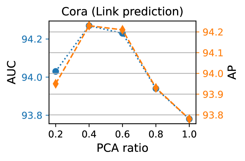
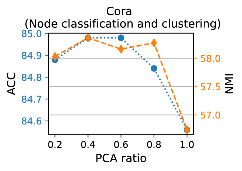
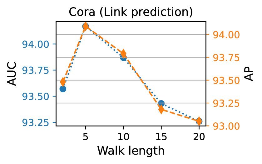
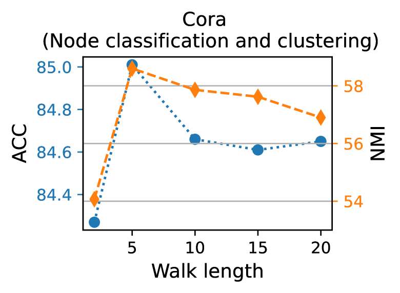
Figure 4 demonstrates the influence of embedding models’ hyper-parameter settings on the proposed framework. Specifically, we choose the compression ratio of PCA and the walk length of node2vec for analysis. The experiments are conducted on the Cora dataset. We can observe that a too-small or too-large PCA ratio could impair the downstream task performance. On the one hand, reconstructing the heavily compressed embedding (ratio=0.2) will lead to the degradation of link prediction and node classification/clustering task performance, possibly due to the reconstructed targets lacking sufficient information. On the other hand, reconstructing the full-size feature matrix (ratio=1.0) will also impair downstream task performance, possibly due to information redundancy. A similar trend can also be observed in the walk length setting. A moderate value (length =5) leads to a decent performance, while a too-small (length =2) or too-large (length =20) value will hurt the performance.

4.4. Ablation Studies on Autoencoder Models

We answer Q3 in this section, where we validate the effectiveness of our proposed learning and mask strategies along with our proposed reconstruction loss design and weight setting strategy.

4.4.1. Evaluation on Learning Strategies

Our GiGaMAE effectively integrates knowledge from multiple targets. For comparison, we design three naive knowledge integration methods, with results in Table 5. In the naive methods, the obtained target embeddings are directly used in downstream tasks after a simple aggregation operation. The aggregation operations include maxpooling, avgpooling, and concatenate. We can observe that these naive methods have poor performance indicating that they are not valid knowledge integration methods compared with the graph masked autoencoder approaches. The impact of different learning objectives is also analyzed in Table 5. For comparison, we replace our proposed MI-based reconstruction loss with MSE, scaled cosine (Hou et al., 2022) and multi-view contrastive loss (Tian et al., 2020), and leave everything else unchanged. The result shows that the scaled cosine and contrastive loss perform better than the MSE. However, neither of them can match the effectiveness of our proposed MI-based learning objective.

4.4.2. Evaluation on Mask Strategies

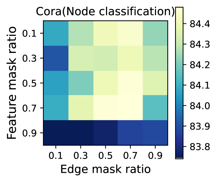
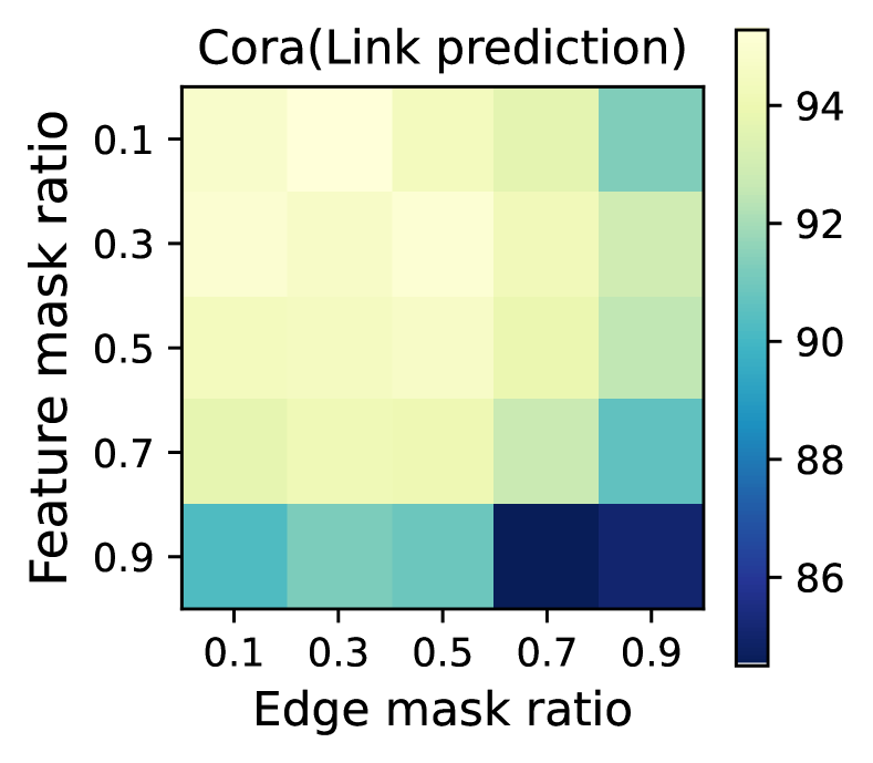
We report the performance of our proposed framework with only one kind of data augmentation, i.e., w/o edge masking and w/o feature masking. The results in Table 5 show that the sole edge or feature mask strategy degrades the downstream performance and generalization ability, which proves the necessity of combining two kinds of mask augmentation together in the generative models. Then we apply different mask ratios on the Cora dataset to see how the downstream performance will change. The result is shown in Figure 5, which shows that a larger mask ratio benefits the node classification task while a smaller mask ratio is preferred for the link prediction task.

4.4.3. Evaluation on Weight Setting

Figure 6 demonstrates the effectiveness of our proposed weight setting strategy. In the WikiCS dataset, the weight $\lambda_{3}$ for the shared knowledge introduced by both node2vec and PCA embeddings is gradually increased for nodes $\mathcal{V}^{B}$ (mask both edges and features). In the Computers dataset, the weight $\lambda_{2}$ for the knowledge solely introduced by the PCA embedding is gradually increased from 1 to 5 for nodes $\mathcal{V}^{F}$ (only mask features). To eliminate interference from other types of nodes, we only use $\mathcal{V}^{B}$ and $\mathcal{V}^{F}$ to calculate the loss in the above cases, respectively. In the left figure, we observe that the model performance improves as we increase $\lambda_{3}$, indicating that the shared knowledge between two targets benefits the learning of $\mathcal{V}^{B}$ nodes, which is consistent with our hypothesis in loss function design. In the right figure, the model performance on $\mathcal{V}^{F}$ nodes improves as $\lambda_{2}$ increases, indicating PCA embedding is more important for self-supervised learning when attributes (of its input graph) are masked.

5. Related Work: Graph Autoencoder

Graph autoencoders typically reconstruct graph components such as edges or features. A traditional way to achieve such reconstruction is to enforce the model to recover the original input graph data. Examples of early research include GAE and VGAE (Kipf and Welling, 2016b), which predict link existence, GALA (Park et al., 2019), which reconstructs features, and GATE (Salehi and Davulcu, 2019), which reconstructs both edges and features. However, these models suffer from overfitting issues and do not produce robust representations (Vincent et al., 2008). To address these challenges, recent works have adopted self-supervised learning strategies, leveraging data augmentation techniques to encourage the model to learn more informative underlying patterns. For example, S2GAE (Tan et al., 2023a) masks edges in the graph and predicts missing links, while MaskGAE (Li et al., 2022) corrupts both edge and path and reconstructs the original edge and degree information. GraphMAE (Hou et al., 2022) utilizes GNN models as the encoder and decoder to reconstruct masked node features, while GraphMAE2 (Hou et al., 2023) introduces latent representation prediction with random re-masking for node attribute reconstruction. Although these models have shown superior performance, they focus on reconstructing specific modality information, limiting their ability to capture more comprehensive knowledge. GPT-GNN (Hu et al., 2020a) tries to overcome this by incorporating both edge masking and feature masking in the training process, aiming to reconstruct joint probability distributions of the graph. However, it assumes a sequential dependency among the generated features/edges that may not exist in real graphs, which generally limits the model applicability. As a result, an effective generative model that seamlessly combines structural and attribute reconstruction is still lacking. To address this issue, we propose the GiGaMAE framework.

6. Conclusion

In this paper, we present a novel framework for Generalizable Graph Masked Autoencoder (GiGaMAE). Our GiGaMAE learns generalizable node representations by reconstructing target embeddings that contain diverse information. We also design a new reconstruction loss based on mutual information, which is flexible to handle knowledge learned by targets individually and shared between multiple targets. We evaluate GiGaMAE via extensive experiments using two efficient target models (node2vec and PCA), where GiGaMAE consistently shows good performance on seven benchmark datasets and three graph learning tasks.

Appendix A Appendix

A.1. Computational Cost Comparison

Our approach requires training the embedding model before reconstruction, resulting in additional computation costs. In this section, we compare the training time of GiGaMA with other baseline models, as shown in Table 6. Our model requires more computation time than GraphMAE due to the extra training time for the embedding models and more advanced learning objective. However, our framework is faster than the contrastive model GCA as we only use a partial graph (masked nodes) for each epoch’s loss calculation, reducing the computation cost.

Table 6. Computation cost (Total seconds for one time run).

datasets	Emb Train		GiGaMAtrain	GiGaMAtotal	GraphMAE	GCA
	PCA	node2vec
Cora	1.22	7.10	8.32	16.64	42.38	27.47
CiteSeer	1.12	3.43	6.53	11.08	10.33	11.34
WikiCS	1.29	2.78	25.50	29.56	57.21	472.08
Computers	1.37	14.63	103.31	119.31	62.82	255.63
Photo	1.31	20.45	121.44	143.20	45.60	141.52
CS	35.58	77.13	247.88	291.38	360.59	314.08
Phy	45.92	140.23	516.18	702.33	391.58	1362.60

A.2. Implementation Details

All experiments are conducted on a workstation with a GPU of NVIDIA A6000. For baselines, we report the baseline model results based on their provided codes with official settings. If their settings are not available, we conduct a hyper-parameter search. The baselines are elevated under the same settings as our model on three downstream tasks. For our graph masked autoencoder, we choose GAT (Veličković et al., 2017) as our encoder model and two-layer MLPs as our projector models. The GiGaMA and embedding model hyper-parameters setting is listed in Table 7.

Table 7. Main hyper-parameters setting.

	Settings	Cora	CiteSeer	WikiCS	Computers	Photo	CS	Physics
GiGaMA	Hidden dimension	512	256	256	512	512	512	512
	Mask_edge	0.4	0.1	0.4	0.4	0.4	0.2	0.2
	Mask_feature	0.4	0.5	0.4	0.4	0.4	0.2	0.2
	$(\tilde{\lambda}_{1},\tilde{\lambda}_{2},\tilde{\lambda}_{3})_{\mathcal{V}^{E}}$	(5,2,6)	(5,2,6)	(5,2,6)	(5,2,6)	(5,2,6)	(5,2,6)	(5,2,6)
	$(\tilde{\lambda}_{1},\tilde{\lambda}_{2},\tilde{\lambda}_{3})_{\mathcal{V}^{F}}$	(2,5,6)	(2,5,6)	(2,5,6)	(2,5,6)	(2,5,6)	(2,5,6)	(2,5,6)
	$(\tilde{\lambda}_{1},\tilde{\lambda}_{2},\tilde{\lambda}_{3})_{\mathcal{V}^{B}}$	(1,1,3)	(1,1,3)	(1,1,3)	(1,1,3)	(1,1,3)	(0,0,1)	(0,0,1)
PCA	Ratio	0.5	0.5	0.5	0.5	0.5	0.9	0.9
Node2vec	Walk length	5	5	10	10	10	10	10
	Context size	5	5	10	10	10	10	10
	Walks per node	5	5	10	10	10	10	10
	Epoch	20	20	20	30	100	200	200

A.3. Theoretical Proof

Lemma A.1.

Chain Rule (1). Given three random variables $X_{1}$, $X_{2}$, and $X_{3}$, we have

$$I(X_{1};X_{2},X_{3})=I(X_{1};X_{3})+I(X_{1};X_{2}|X_{3}).$$

Proof.

Using the chain rule for entropy, we first can have:

$$I(X_{1};X_{2}\mid X_{3}) =H(X_{1},X_{3})+H(X_{2},X_{3})-H(X_{1},X_{2},X_{3})-H(X_{3})$$

$$=H(X_{1}\mid X_{3})+H(X_{2}\mid X_{3})-H(X_{1},X_{2}\mid X_{3}).$$

Then the above can be re-written to

$$I(X_{1};X_{2}|X_{3})=I(X_{1};X_{2},X_{3})-I(X_{1};X_{3}).$$

Rearrange the above equation, we can have

$$I(X_{1};X_{2},X_{3})=I(X_{1};X_{3})+I(X_{1};X_{2}|X_{3}).$$

∎

Lemma A.2.

Chain Rule (2). Given three random variables $X_{1}$, $X_{2}$, and $X_{3}$, we have:

$$I(X_{1};X_{2};X_{3})=I(X_{1};X_{2})+I(X_{1};X_{3})-I(X_{1};X_{2},X_{3}).$$

Proof.

By definition, the multivariate mutual information is defined as:

$$I(X_{1};X_{2};X_{3})=I(X_{1};X_{2})-I(X_{1};X_{2}\mid X_{3}).$$

So according to Equation (3), we can get:

$$I(X_{1};X_{2};X_{3})=I(X_{1};X_{2})-(I(X_{1};X_{2},X_{3})-I(X_{1};X_{3}))$$

$$=I(X_{1};X_{2})+I(X_{1};X_{3})-I(X_{1};X_{2},X_{3}).$$

∎

References

- (1)
- Abdi and Williams (2010) Hervé Abdi and Lynne J Williams. 2010. Principal component analysis. Wiley interdisciplinary reviews: computational statistics 2, 4 (2010), 433–459.
- Ahmed et al. (2013) Amr Ahmed, Nino Shervashidze, Shravan Narayanamurthy, Vanja Josifovski, and Alexander J Smola. 2013. Distributed large-scale natural graph factorization. In Proceedings of the 22nd international conference on World Wide Web. 37–48.
- Cai et al. (2021) Lei Cai, Zhengzhang Chen, Chen Luo, Jiaping Gui, Jingchao Ni, Ding Li, and Haifeng Chen. 2021. Structural temporal graph neural networks for anomaly detection in dynamic graphs. In Proceedings of the 30th ACM international conference on Information & Knowledge Management. 3747–3756.
- Candès et al. (2011) Emmanuel J Candès, Xiaodong Li, Yi Ma, and John Wright. 2011. Robust principal component analysis? Journal of the ACM (JACM) 58, 3 (2011), 1–37.
- Chen et al. (2020) Ting Chen, Simon Kornblith, Mohammad Norouzi, and Geoffrey Hinton. 2020. A simple framework for contrastive learning of visual representations. In ICML. PMLR, 1597–1607.
- Csiszár (1975) Imre Csiszár. 1975. I-divergence geometry of probability distributions and minimization problems. The annals of probability (1975), 146–158.
- Devlin et al. (2018) Jacob Devlin, Ming-Wei Chang, Kenton Lee, and Kristina Toutanova. 2018. Bert: Pre-training of deep bidirectional transformers for language understanding. arXiv preprint arXiv:1810.04805 (2018).
- Fan et al. (2019) Wenqi Fan, Yao Ma, Qing Li, Yuan He, Eric Zhao, Jiliang Tang, and Dawei Yin. 2019. Graph neural networks for social recommendation. In The world wide web conference. 417–426.
- Fey and Lenssen (2019) Matthias Fey and Jan E. Lenssen. 2019. Fast Graph Representation Learning with PyTorch Geometric. In ICLR Workshop on Representation Learning on Graphs and Manifolds.
- Gabrié et al. (2018) Marylou Gabrié, Andre Manoel, Clément Luneau, Nicolas Macris, Florent Krzakala, Lenka Zdeborová, et al. 2018. Entropy and mutual information in models of deep neural networks. NIPS 31 (2018).
- Grover and Leskovec (2016) Aditya Grover and Jure Leskovec. 2016. node2vec: Scalable feature learning for networks. In Proceedings of the 22nd ACM SIGKDD international conference on Knowledge discovery and data mining. 855–864.
- Guan et al. (2023) Zihan Guan, Mengnan Du, and Ninghao Liu. 2023. XGBD: Explanation-Guided Graph Backdoor Detection. arXiv preprint arXiv:2308.04406 (2023).
- Hassani and Khasahmadi (2020) Kaveh Hassani and Amir Hosein Khasahmadi. 2020. Contrastive multi-view representation learning on graphs. In ICML. PMLR, 4116–4126.
- He et al. (2022) Kaiming He, Xinlei Chen, Saining Xie, Yanghao Li, Piotr Dollár, and Ross Girshick. 2022. Masked autoencoders are scalable vision learners. In Proceedings of the IEEE/CVF Conference on Computer Vision and Pattern Recognition. 16000–16009.
- Hou et al. (2023) Zhenyu Hou, Yufei He, Yukuo Cen, Xiao Liu, Yuxiao Dong, Evgeny Kharlamov, and Jie Tang. 2023. GraphMAE2: A Decoding-Enhanced Masked Self-Supervised Graph Learner. arXiv preprint arXiv:2304.04779 (2023).
- Hou et al. (2022) Zhenyu Hou, Xiao Liu, Yuxiao Dong, Chunjie Wang, Jie Tang, et al. 2022. GraphMAE: Self-Supervised Masked Graph Autoencoders. arXiv preprint arXiv:2205.10803 (2022).
- Hu et al. (2020b) Ruiqi Hu, Shirui Pan, Guodong Long, Qinghua Lu, Liming Zhu, and Jing Jiang. 2020b. Going deep: Graph convolutional ladder-shape networks. In Proceedings of the AAAI Conference on Artificial Intelligence, Vol. 34. 2838–2845.
- Hu et al. (2020a) Ziniu Hu, Yuxiao Dong, Kuansan Wang, Kai-Wei Chang, and Yizhou Sun. 2020a. Gpt-gnn: Generative pre-training of graph neural networks. In Proceedings of the 26th ACM SIGKDD International Conference on Knowledge Discovery & Data Mining. 1857–1867.
- Huang et al. (2021) Yu Huang, Chenzhuang Du, Zihui Xue, Xuanyao Chen, Hang Zhao, and Longbo Huang. 2021. What makes multi-modal learning better than single (provably). NIPS 34 (2021), 10944–10956.
- Kipf and Welling (2016a) Thomas N Kipf and Max Welling. 2016a. Semi-supervised classification with graph convolutional networks. arXiv preprint arXiv:1609.02907 (2016).
- Kipf and Welling (2016b) Thomas N Kipf and Max Welling. 2016b. Variational graph auto-encoders. arXiv preprint arXiv:1611.07308 (2016).
- Kirillov et al. (2023) Alexander Kirillov, Eric Mintun, Nikhila Ravi, Hanzi Mao, Chloe Rolland, Laura Gustafson, Tete Xiao, Spencer Whitehead, Alexander C Berg, Wan-Yen Lo, et al. 2023. Segment anything. arXiv preprint arXiv:2304.02643 (2023).
- Li et al. (2022) Jintang Li, Ruofan Wu, Wangbin Sun, Liang Chen, Sheng Tian, Liang Zhu, Changhua Meng, Zibin Zheng, and Weiqiang Wang. 2022. MaskGAE: masked graph modeling meets graph autoencoders. arXiv preprint arXiv:2205.10053 (2022).
- Lin et al. (2021) Baijiong Lin, Feiyang Ye, and Yu Zhang. 2021. A closer look at loss weighting in multi-task learning. arXiv preprint arXiv:2111.10603 (2021).
- Mernyei and Cangea (2020) Péter Mernyei and Cătălina Cangea. 2020. Wiki-cs: A wikipedia-based benchmark for graph neural networks. arXiv preprint arXiv:2007.02901 (2020).
- Oord et al. (2018) Aaron van den Oord, Yazhe Li, and Oriol Vinyals. 2018. Representation learning with contrastive predictive coding. arXiv preprint arXiv:1807.03748 (2018).
- Park et al. (2019) Jiwoong Park, Minsik Lee, Hyung Jin Chang, Kyuewang Lee, and Jin Young Choi. 2019. Symmetric graph convolutional autoencoder for unsupervised graph representation learning. In Proceedings of the IEEE/CVF International Conference on Computer Vision. 6519–6528.
- Paszke et al. (2019) Adam Paszke, Sam Gross, Francisco Massa, Adam Lerer, James Bradbury, Gregory Chanan, Trevor Killeen, Zeming Lin, Natalia Gimelshein, Luca Antiga, et al. 2019. Pytorch: An imperative style, high-performance deep learning library. NIPS 32 (2019).
- Perozzi et al. (2014) Bryan Perozzi, Rami Al-Rfou, and Steven Skiena. 2014. Deepwalk: Online learning of social representations. In Proceedings of the 20th ACM SIGKDD international conference on Knowledge discovery and data mining. 701–710.
- Poole et al. (2019) Ben Poole, Sherjil Ozair, Aaron Van Den Oord, Alex Alemi, and George Tucker. 2019. On variational bounds of mutual information. In ICML. PMLR, 5171–5180.
- Salehi and Davulcu (2019) Amin Salehi and Hasan Davulcu. 2019. Graph attention auto-encoders. arXiv preprint arXiv:1905.10715 (2019).
- Salmon et al. (2014) Joseph Salmon, Zachary Harmany, Charles-Alban Deledalle, and Rebecca Willett. 2014. Poisson noise reduction with non-local PCA. Journal of mathematical imaging and vision 48, 2 (2014), 279–294.
- Shannon (1948) Claude Elwood Shannon. 1948. A mathematical theory of communication. The Bell system technical journal 27, 3 (1948), 379–423.
- Shchur et al. (2018) Oleksandr Shchur, Maximilian Mumme, Aleksandar Bojchevski, and Stephan Günnemann. 2018. Pitfalls of graph neural network evaluation. arXiv preprint arXiv:1811.05868 (2018).
- Shi et al. (2023a) Yucheng Shi, Hehuan Ma, Wenliang Zhong, Gengchen Mai, Xiang Li, Tianming Liu, and Junzhou Huang. 2023a. Chatgraph: Interpretable text classification by converting chatgpt knowledge to graphs. arXiv preprint arXiv:2305.03513 (2023).
- Shi et al. (2023b) Yucheng Shi, Kaixiong Zhou, and Ninghao Liu. 2023b. ENGAGE: Explanation Guided Data Augmentation for Graph Representation Learning. arXiv preprint arXiv:2307.01053 (2023).
- Tan et al. (2019) Qiaoyu Tan, Ninghao Liu, and Xia Hu. 2019. Deep representation learning for social network analysis. Frontiers in big Data 2 (2019), 2.
- Tan et al. (2023a) Qiaoyu Tan, Ninghao Liu, Xiao Huang, Soo-Hyun Choi, Li Li, Rui Chen, and Xia Hu. 2023a. S2GAE: Self-Supervised Graph Autoencoders are Generalizable Learners with Graph Masking. In Proceedings of the Sixteenth ACM International Conference on Web Search and Data Mining. 787–795.
- Tan et al. (2021a) Qiaoyu Tan, Jianwei Zhang, Ninghao Liu, Xiao Huang, Hongxia Yang, Jingren Zhou, and Xia Hu. 2021a. Dynamic memory based attention network for sequential recommendation. In Proceedings of the AAAI conference on artificial intelligence, Vol. 35. 4384–4392.
- Tan et al. (2021b) Qiaoyu Tan, Jianwei Zhang, Jiangchao Yao, Ninghao Liu, Jingren Zhou, Hongxia Yang, and Xia Hu. 2021b. Sparse-interest network for sequential recommendation. In Proceedings of the 14th ACM international conference on web search and data mining. 598–606.
- Tan et al. (2023b) Qiaoyu Tan, Xin Zhang, Xiao Huang, Hao Chen, Jundong Li, and Xia Hu. 2023b. Collaborative Graph Neural Networks for Attributed Network Embedding. IEEE Transactions on Knowledge and Data Engineering (2023).
- Tan et al. (2023c) Qiaoyu Tan, Xin Zhang, Ninghao Liu, Daochen Zha, Li Li, Rui Chen, Soo-Hyun Choi, and Xia Hu. 2023c. Bring your own view: Graph neural networks for link prediction with personalized subgraph selection. In Proceedings of the Sixteenth ACM International Conference on Web Search and Data Mining. 625–633.
- Thakoor et al. (2021a) Shantanu Thakoor, Corentin Tallec, Mohammad Gheshlaghi Azar, Mehdi Azabou, Eva L Dyer, Remi Munos, Petar Veličković, and Michal Valko. 2021a. Large-scale representation learning on graphs via bootstrapping. arXiv preprint arXiv:2102.06514 (2021).
- Thakoor et al. (2021b) Shantanu Thakoor, Corentin Tallec, Mohammad Gheshlaghi Azar, Rémi Munos, Petar Veličković, and Michal Valko. 2021b. Bootstrapped representation learning on graphs. In ICLR 2021 Workshop.
- Tian et al. (2019) Yonglong Tian, Dilip Krishnan, and Phillip Isola. 2019. Contrastive representation distillation. arXiv preprint arXiv:1910.10699 (2019).
- Tian et al. (2020) Yonglong Tian, Dilip Krishnan, and Phillip Isola. 2020. Contrastive multiview coding. In European conference on computer vision. Springer, 776–794.
- Tishby et al. (2000) Naftali Tishby, Fernando C Pereira, and William Bialek. 2000. The information bottleneck method. arXiv preprint physics/0004057 (2000).
- Tschannen et al. (2019) Michael Tschannen, Josip Djolonga, Paul K Rubenstein, Sylvain Gelly, and Mario Lucic. 2019. On mutual information maximization for representation learning. arXiv preprint arXiv:1907.13625 (2019).
- Veličković et al. (2017) Petar Veličković, Guillem Cucurull, Arantxa Casanova, Adriana Romero, Pietro Lio, and Yoshua Bengio. 2017. Graph attention networks. arXiv preprint arXiv:1710.10903 (2017).
- Veličković et al. (2018) Petar Veličković, William Fedus, William L Hamilton, Pietro Liò, Yoshua Bengio, and R Devon Hjelm. 2018. Deep graph infomax. arXiv preprint arXiv:1809.10341 (2018).
- Vincent et al. (2008) Pascal Vincent, Hugo Larochelle, Yoshua Bengio, and Pierre-Antoine Manzagol. 2008. Extracting and composing robust features with denoising autoencoders. In Proceedings of the 25th ICML. 1096–1103.
- Wang et al. (2017) Chun Wang, Shirui Pan, Guodong Long, Xingquan Zhu, and Jing Jiang. 2017. Mgae: Marginalized graph autoencoder for graph clustering. In Proceedings of the 2017 ACM on Conference on Information and Knowledge Management. 889–898.
- Wang et al. (2016) Yasi Wang, Hongxun Yao, and Sicheng Zhao. 2016. Auto-encoder based dimensionality reduction. Neurocomputing 184 (2016), 232–242.
- Wei et al. (2022) Chen Wei, Haoqi Fan, Saining Xie, Chao-Yuan Wu, Alan Yuille, and Christoph Feichtenhofer. 2022. Masked feature prediction for self-supervised visual pre-training. In Proceedings of the IEEE/CVF Conference on Computer Vision and Pattern Recognition. 14668–14678.
- Yang et al. (2016) Zhilin Yang, William Cohen, and Ruslan Salakhudinov. 2016. Revisiting semi-supervised learning with graph embeddings. In ICML. PMLR, 40–48.
- You et al. (2020) Yuning You, Tianlong Chen, Yongduo Sui, Ting Chen, Zhangyang Wang, and Yang Shen. 2020. Graph contrastive learning with augmentations. NIPS 33 (2020), 5812–5823.
- Yu et al. (2020) Tianhe Yu, Saurabh Kumar, Abhishek Gupta, Sergey Levine, Karol Hausman, and Chelsea Finn. 2020. Gradient surgery for multi-task learning. NIPS 33 (2020), 5824–5836.
- Zheng et al. (2021) Sixiao Zheng, Jiachen Lu, Hengshuang Zhao, Xiatian Zhu, Zekun Luo, Yabiao Wang, Yanwei Fu, Jianfeng Feng, Tao Xiang, Philip HS Torr, et al. 2021. Rethinking semantic segmentation from a sequence-to-sequence perspective with transformers. In Proceedings of the IEEE/CVF conference on computer vision and pattern recognition. 6881–6890.
- Zhou et al. (2021) Huachi Zhou, Qiaoyu Tan, Xiao Huang, Kaixiong Zhou, and Xiaoling Wang. 2021. Temporal augmented graph neural networks for session-based recommendations. In Proceedings of the 44th International ACM SIGIR conference on research and development in information retrieval. 1798–1802.
- Zhou et al. (2022) Shuang Zhou, Xiao Huang, Ninghao Liu, Qiaoyu Tan, and Fu-Lai Chung. 2022. Unseen anomaly detection on networks via multi-hypersphere learning. In Proceedings of the 2022 SIAM International Conference on Data Mining (SDM). SIAM, 262–270.
- Zhu et al. (2020) Yanqiao Zhu, Yichen Xu, Feng Yu, Qiang Liu, Shu Wu, and Liang Wang. 2020. Deep graph contrastive representation learning. arXiv preprint arXiv:2006.04131 (2020).
- Zhu et al. (2021) Yanqiao Zhu, Yichen Xu, Feng Yu, Qiang Liu, Shu Wu, and Liang Wang. 2021. Graph contrastive learning with adaptive augmentation. In Proceedings of the Web Conference 2021. 2069–2080.