Critical enhancement of the spin Hall effect by spin fluctuations

Abstract

The spin Hall (SH) effect, the conversion of the electric current to the spin current along the transverse direction, relies on the relativistic spin-orbit coupling (SOC). Here, we develop microscopic mechanisms of the SH effect in magnetic metals, where itinerant electrons are coupled with localized magnetic moments via the Hund exchange interaction and the SOC. Both antiferromagnetic metals and ferromagnetic metals are considered. It is shown that the spin Hall conductivity can be significantly enhanced by the spin fluctuation when approaching the magnetic transition temperature of both cases. For antiferromagnetic metals, the pure SHE appears in entire temperature range, while for ferromagnetic metals, the pure SHE is expected to be replaced by the anomalous Hall effect below the transition temperature. We also discuss possible experimental realizations and the effect of the quantum criticality when the antiferromagnetic transition temperature is tuned to zero temperature.

Introduction

The spin Hall (SH) effect [1, 2] and its reciprocal effect, the inverse SH effect [3], are among the most important components for the spintronic application [4] because they allow the conversion between charge current and pure spin current electrically. A variety of phenomena have been envisioned [5, 6]. The SH effect and the anomalous Hall (AH) effect  [7] are both rooted in the relativistic spin-orbit coupling (SOC), and these effects are traditionally understood as arising from intrinsic mechanisms, i.e., band effects, [8, 9] or extrinsic mechanisms, i.e., impurity/disorder effects [10, 11, 12, 13] and interfaces [14].

There have appeared a number of proposals of the extrinsic mechanisms of the SH effect utilizing excitations or fluctuations in solids, such as phonons [15, 16, 17]. Identifying new mechanisms thus opens up a new research avenue and hereby helps to improve the efficiency of the SH effect, which remains small for practical applications [18]. Recently, the current authors proposed extrinsic mechanisms focusing on the spin fluctuation (SF) in nearly ferromagnetic (FM) disordered systems [19]. In these mechanisms, the critical SF associated with the zero-temperature FM quantum critical point (QCP) plays a fundamental role. It was predicted that the SH conductivity $\sigma_{SH}$ is maximized at nonzero temperature when approaching the QCP. When the FM transition temperature $T_{C}$ is finite, the pure SH effect is replaced by the AH effect below $T_{C}$, thus limiting the operation temperature range of the SH effect. This limitation could be lifted when the antiferromagnetic (AFM) SF is considered because the net magnetic moment is absent even below the AFM transition temperature $T_{N}$. From the study of itinerant electron magnetism [20], it has been recognized that the FM SF and the AFM SF provide qualitatively different behavior in electronic specific heat, conductivity, etc [22, 23, 21]. Thus, the SH effect could be another example that highlights the difference between FM SF and AFM SF.

While the SH effect due to the FM critical SF has not been experimentally examined, yet, Refs. [24, 25, 26] examined the SH effect in FM alloys with finite $T_{C}$. In Ref. [24], Wei et al. reported that the temperature dependence of the inverse SH resistance of Ni-Pd alloys follows the uniform second-order nonlinear susceptibility $\chi_{2}$, but the inverse SH resistance has peaks above and below the Curie temperature and changes its sign at $T_{C}$. This behavior is consistent with the theoretical prediction in Ref. [27], which used a static mean field approximation to the model proposed by Kondo [28]. On the other hand in Ref. [25], Ou et al. reported that the inverse SH effect of Fe-Pt alloys is maximized near $T_{C}$ as if it follows the uniform linear susceptibility. More recently, Wu et al. reported similar effects using Ni-Cu alloys [26]. For AFM systems, early work on Cr has already reported the large SH effects [29, 30]. Recently, Fang and coworkers found that the SH conductivity in metallic Cr is enhanced when temperature is approaching the Néel temperature $T_{N}$ [31], suggesting the AFM SF as the main mechanism of the SH effect. However, the effect of AFM SF to the SH effect has not been theoretically addressed.

The main purpose of this work is to develop the theoretical description of the SH effect in magnetic metallic systems by the SF when the magnetic transition temperature ($T_{C}$ or $T_{N}$) is finite. Our theory is based on a microscopic model describing the coupling between itinerant electrons and localized magnetic moments by Kondo [28] and the self-consistent renormalization theory describing the fluctuation of localized moments by Moriya [20]. The main difference between AFM systems and FM systems is that the AFM ordering or correlation is characterized by the nonzero magnetic wave vector $\mathbf{Q}$. Thus, itinerant electrons scattered by the AFM SF gain or lose corresponding momenta. Our theory takes into account this momentum conservation appropriately. Despite this difference, it is demonstrated that the SH conductivity is enhanced as temperature is approaching $T_{C}$ for FM systems or $T_{N}$ for AFM systems. The result for the AFM systems strongly supports the conjecture made in Ref. [31]. We highlight the qualitatively different behavior between the AFM SF and the FM SF near the finite-temperature phase transition and near the QCP.

Results

Theoretical model and formalism We start from setting up our theoretical tools. First, we introduce the $s$-$d$ Hamiltonian, which is modified from the original form developed by Kondo [28]. This clarifies the scattering mechanism for the SH conductivity. Second, we set up the Gaussian action, which describes the SF based on the self-consistent renormalization theory by Moriya [20].

In this work, we consider three-dimensional systems. The $s$-$d$ Hamiltonian is written as $H=H_{0}+H_{K}$. Here, the non-interacting itinerant electron part is described by $H_{0}=\sum_{\mathbf{k},\nu}\varepsilon_{\mathbf{k}}a_{\mathbf{k}\nu}^{\dagger}a_{\mathbf{k}\nu}$, where $\varepsilon_{\mathbf{k}}$ is an energy eigenvalue at momentum $\mathbf{k}$ given by $\varepsilon_{\mathbf{k}}=\frac{\hbar^{2}k^{2}}{2m}-\varepsilon_{F}$ with the Fermi energy $\varepsilon_{F}$ and the carrier effective mass $m$, and $a_{\mathbf{k}\nu}^{({\dagger})}$ is an annihilation (creation) operator of an electron at momentum $\mathbf{k}$ with the spin index $\nu$. This electronic part of the Hamiltonian is assumed to be unrenormalized [20]. However, as discussed briefly later, going beyond this assumption is necessary especially near the finite temperature phase transition. The $s$-$d$ coupling term in the original model has a mixed representation of momentum of conduction electrons and real-space coordinate of localized magnetic moments [28, 32]. For magnetic metallic systems, where localized magnetic moments form a periodic lattice and conduction electrons hop through the same lattice sites, it is more convenient to express a model Hamiltonian entirely in the momentum space as

$$H_{K}\!\!\! = \!\!\!-\frac{1}{\sqrt{N}}\sum_{\mathbf{k},\mathbf{k}^{\prime}}\sum_{\nu,\nu^{\prime}}a_{\mathbf{k}\nu}^{\dagger}a_{\mathbf{k}^{\prime}\nu^{\prime}}\Biggl{[}2(\mathbf{J}_{\mathbf{k}-\mathbf{k}^{\prime}}\cdot\mathbf{s}_{\nu\nu^{\prime}})$$ (1)

$$\times \!\!\!\bigl{\{}{\cal F}_{0}+2{\cal F}_{1}(\mathbf{k}\cdot\mathbf{k}^{\prime})\bigr{\}}+i{\cal F}_{2}\mathbf{J}_{\mathbf{k}-\mathbf{k}^{\prime}}\cdot(\mathbf{k}^{\prime}\times\mathbf{k})$$

$$+ \!\!\!\frac{i}{\sqrt{N}}\sum_{\mathbf{p}}{\cal F}_{3}\biggl{\{}(\mathbf{J}_{\mathbf{p}}\cdot\mathbf{s}_{\nu\nu^{\prime}})\bigl{(}\mathbf{J}_{\mathbf{k}-\mathbf{k}^{\prime}-\mathbf{p}}\cdot(\mathbf{k}^{\prime}\times\mathbf{k})\bigr{)}$$

$$+ \!\!\!\bigl{(}\mathbf{J}_{\mathbf{p}}\cdot(\mathbf{k}^{\prime}\times\mathbf{k})\bigr{)}(\mathbf{J}_{\mathbf{k}-\mathbf{k}^{\prime}-\mathbf{p}}\cdot\mathbf{s}_{\nu\nu^{\prime}})$$

$$- \!\!\!\frac{2}{3}(\mathbf{J}_{\mathbf{p}}\cdot\mathbf{J}_{\mathbf{k}-\mathbf{k}^{\prime}-\mathbf{p}})\bigl{(}\mathbf{s}_{\nu\nu^{\prime}}\cdot(\mathbf{k}^{\prime}\times\mathbf{k})\bigr{)}\biggr{\}}\Biggr{]}.$$

Here, $\mathbf{s}_{\nu\nu^{\prime}}=\frac{1}{2}\mbox{\boldmath$\sigma$}_{\nu\nu^{\prime}}$ is the spin of a conduction electron with the Pauli matrices $\sigma$. $N$ is the total number of lattice sites. $\mathbf{J}_{\mathbf{p}}$ is the Fourier transform of a local spin moment $\mathbf{J}_{n}$ at position $\mathbf{R}_{n}$ defined by $\mathbf{J}_{\mathbf{p}}=\frac{1}{\sqrt{N}}\sum_{n}\mathbf{J}_{n}e^{-i\mathbf{p}\cdot\mathbf{R}_{n}}$. Parameters ${\cal F}_{l}$ [19] are related to $F_{l}$ defined in Ref. [28]. ${\cal F}_{0,1}$ terms correspond to the standard $s$-$d$ exchange interaction or Hund coupling as depicted in Fig. 1 (a). ${\cal F}_{2,3}$ terms represent the exchange of angular momentum between a conduction electron and a local moment. These ${\cal F}_{2,3}$ terms are odd (linear or cubic)-order in $\mathbf{J}_{n}$ and $\mathbf{s}$ and induce the electron deflection depending on the direction of $\mathbf{J}_{n}$ or $\mathbf{s}$. More precisely, the ${\cal F}_{2}$ term and the ${\cal F}_{3}$ term generate the side-jump and the skew-scattering contributions to the SH conductivity, respectively, as depicted in Fig. 1 (b) and (c). From Eq. (S1) and the position operator $\mathbf{r}$, the velocity operator is obtained as $\mathbf{v}=(i/\hbar)[H_{K},\mathbf{r}]$. The anomalous velocity, the main source of the side-jump contribution, arises from the ${\cal F}_{2}$ term (see Ref. [32] for details).

From Eq. (S1), one can notice the main difference from FM alloy systems [19]. Since itinerant electrons and localized moments share the same lattice structure, their coupling does not have a phase factor such as $e^{i\mathbf{p}\cdot(\mathbf{R}_{n}-\mathbf{R}_{n^{\prime}})}$, where $\mathbf{R}_{n}$ is the position of the localized moment $\mathbf{J}_{n}$. Therefore, the SF could contribute to the SH effect even if it has characteristic momentum $\mathbf{Q}\neq\mathbf{0}$, such as in AFM systems, without introducing destructive effects. Otherwise, averaging over the lattice coordinate would lead to zero SH effect as $\langle e^{i\mathbf{Q}\cdot(\mathbf{R}_{n}-\mathbf{R}_{n^{\prime}})}\rangle\approx 0$.

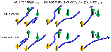
Figure 1: Schematic view of the Kondo model. (a) Spin dependent scattering by ${\cal F}_{0,1}$ terms, (b) anomalous velocity induced by ${\cal F}_{2}$ terms, and (c) skew scattering by ${\cal F}_{3}$terms. Yellow arrows indicate conduction electrons, and green arrows indicate local moments. In the ${\cal F}_{2(3)}$ scattering processes, the electron deflection depends on the direction of the local moment (the electron spin), leading to the side-jump (skew-scattering) contribution to $\sigma_{SH}$.

To describe the fluctuation of localized moments $\mathbf{J}_{n}$, we adopt a generic Gaussian action given by [20, 33, 34, 35],

$$A_{Gauss}=\frac{1}{2}\sum_{\mathbf{p},l}D^{-1}_{\mathbf{p}}(i\omega_{l})\,{\mathbf{J}}_{\mathbf{p}}(i\omega_{l})\cdot{\mathbf{J}}_{-\mathbf{p}}(-i\omega_{l})$$ (2)

with

$$D_{\mathbf{p}}(i\omega_{l})=\frac{1}{\delta+A|\mathbf{p}-\mathbf{Q}|^{2}+|\omega_{l}|/\Gamma_{\mathbf{p}}}.$$ (3)

Here, $\mathbf{J}_{\mathbf{p}}(i\omega_{l})$ is a space and imaginary-time $\tau$ Fourier transform of $\mathbf{J}_{n}(\tau)$, where we made the $\tau$ dependence explicit, and $\omega_{l}=2l\pi T$ is the bosonic Matsubara frequency. Parameter $A$ is introduced as a constant so that $A|\mathbf{p}-\mathbf{Q}|^{2}$ has the unit of energy, and $\delta$ is the distance from the magnetic transition temperature and is related to the magnetic correlation length as $\xi\propto\delta^{-1/2}$ at $T>T_{N,C}$ and to the ordered magnetic moment as $M(T)\propto\delta^{1/2}$ at $T<T_{N,C}$. $\Gamma_{\mathbf{p}}$ represents the Landau damping, whose momentum dependence is neglected for AFM systems, $\Gamma_{\mathbf{p}}=\Gamma$, since it is weak near the magnetic wave vector $\mathbf{Q}$. For FM systems with $\mathbf{Q}=\mathbf{0}$, the damping term has a momentum dependence as $\Gamma_{\mathbf{p}}=\Gamma p$. With impurity scattering or disorder, $\Gamma_{\mathbf{p}}$ remains finite below a cutoff momentum $|\mathbf{p}|\leq q_{c}$ as $\Gamma_{\mathbf{p}}=\Gamma q_{c}$.

Theoretical analyses based on this model have been successful to explain many experimental results on itinerant magnets [20]. In principle, $\delta$ depends on temperature and is determined by solving self-consistent equations for a full model including non-Gaussian terms [33, 34, 20, 35, 36]. However, the temperature dependence of $\delta$ is know for the following three cases in three dimension. I: $\delta\propto(T-T_{N,C})$ at $T\gtrsim T_{N,C}$, II: $\delta\propto M^{2}(T)\propto T_{N,C}-T$ at $T\lesssim T_{N,C}$, and III: $\delta\propto T^{3/2}$ at $T\sim 0$ when $T_{N}\rightarrow 0$, i.e., approaching the QCP. For FM with impurity scattering or disorder $\delta\propto T^{3/2}$ at $T\sim 0$ when $T_{C}\rightarrow 0$, while for clean FM $\delta\propto T^{4/3}$.

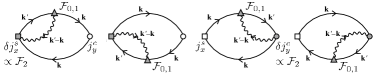
Figure 2: Diagrammatic representation for the side-jump contribution. Solid (wavy) lines are the electron Green’s functions (the SF propagators). Squares (circles) are the spin (charge) current vertices, with filled symbols representing the velocity correction with ${\cal F}_{2}$, i.e., side jump. Filled triangles are the interaction vertices with ${\cal F}_{0,1}$.

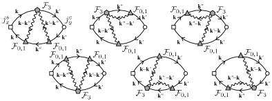
Figure 3: Diagrammatic representation for the skew-scattering contribution. Filled pentagons are the interaction vertices with ${\cal F}_{3}$. The definitions of the other symbols or lines are the same as in Fig. 2.

Spin-Hall conductivity With the above preparations, we analyze the SH conductivity using the Matsubara formalism, by which one can take the dynamical SF into account via a diagramatic technique as described in Ref. [32]. Here, the frequency-dependent SH conductivity is considered as $\sigma_{SH}(i\Omega_{l})$. $\Omega_{l}$ is the bosonic Matsubara frequency, which is analytically continued to real frequency as $i\Omega_{l}\rightarrow\Omega+i0^{+}$ at the end of the analysis, and then the DC limit, $\Omega\rightarrow 0$, is taken to obtain $\sigma_{SH}$. Based on the diagrammatic representations in Figs. 2 and 3, $\sigma_{SH}$ is expressed in terms of electron Green’s function $G$ and the propagator $D$ of the longitudinal SF. While the transverse SFs or spin wave excitatiosn exist below the magnetic transition temperature, the scattering of electrons by such SFs does not show a critical behavior [37, 38], and its contribution is expected to be small. Therefore, for our analysis, we consider only longitudinal SFs below $T_{N,C}$.

We first focus on the SH effect by the AFM SF. By carrying out the Matsubara summations, the energy integrals and the momentum summations as detailed in Ref. [32], we find

$$\sigma^{side\,jump}_{AFM,SH}\approx\frac{e^{2}m\tau_{\mathbf{k}}}{2\pi^{3}\hbar^{4}|\mathbf{Q}|}\,A_{AFM}^{side\,jump}\,\tilde{I}_{AFM}(T,\delta)$$ (4)

for the side-jump contribution and

$$\sigma^{skew\,scat.}_{AFM,SH}\approx\frac{e^{2}\tau_{\mathbf{k}}^{2}\,\Gamma\,\delta}{2\pi^{2}\hbar^{3}|\mathbf{Q}|}\,A_{AFM}^{skew\,scat.}\,I_{AFM}^{2}(T,\delta)$$ (5)

for the skew-scatting contribution. In both cases, $\tau_{\mathbf{k}}$ is the carrier lifetime on the Fermi surface at special momenta $\mathbf{k}$ that satisfy the nesting condition. Such momenta $\mathbf{k}$ form loops on the Fermi surface. With the parabolic band, the carrier lifetime due to the AFM SF along such loops is independent of momentum [32]. The momentum dependence of the carrier lifetime due to other effects, such as disorder and phonons, is weak. Thus, we assume that $\tau_{\mathbf{k}}$ is a constant. The functions $\tilde{I}_{AFM}(T,\delta)$ and $I_{AFM}(T,\delta)$ defined in Ref. [32] represent the coupling between conduction electrons and the dynamical SF. $A_{AFM}^{side\,jump}$ and $A_{AFM}^{skew\,scatt.}$ are constants defined by the integrals over the azimuth angle of momentum $\mathbf{k}$ measured from the direction of $\mathbf{Q}$ as described in Ref. [32]. Since the angle integrals give only geometrical factors of ${\cal O}(1)$, $A_{AFM}^{side\,jump}\approx{\cal F}_{0}{\cal F}_{2}k_{F}^{2}$ and $A_{AFM}^{skew\,scatt.}\approx{\cal F}_{0}^{2}{\cal F}_{3}k_{F}^{4}$.

Similarly, the SH conductivity due to the FM SF is obtained (for details, see Ref. [32]) as

$$\sigma^{side\,jump}_{FM,SH}\approx\frac{2e^{2}\tau_{\mathbf{k}}}{m}\,A_{FM}^{side\,jump}\,I_{FM}(T,\delta)$$ (6)

for the side-jump contribution and

$$\sigma^{skew\,scat.}_{FM,SH}\approx\frac{4e^{2}\hbar\tau_{\mathbf{k}}^{2}}{m^{2}}\,A_{FM}^{skew\,scat.}\,I_{FM}^{2}(T,\delta)$$ (7)

for the skew-scatting contribution. Here, $\tau_{\mathbf{k}}$ is the carrier lifetime on the Fermi surface, and the constants $A_{FM}^{side\,jump}$ and $A_{FM}^{skew\,scatt.}$ are given by $A_{FM}^{side\,jump}\approx\frac{mk_{F}^{3}}{\pi^{2}\hbar}{\cal F}_{0}{\cal F}_{2}$ and $A_{FM}^{skew\,scatt.}\approx\frac{mk_{F}^{5}}{\pi^{2}\hbar^{2}}{\cal F}_{0}^{2}{\cal F}_{3}$, respectively. The function $I_{FM}(T,\delta)$ is defined in Ref. [32].

Table 1: $T$ dependence of $\sigma_{SH}$. An additional $T$ dependence appears via the carrier lifetime $\tau_{\mathbf{k}}$.

$T$ regime		$\sigma_{AFM,SH}^{side\,jump}$	$\sigma_{AFM,SH}^{skew\,scatt.}$	$\sigma_{FM,SH}^{side\,jump}$	$\sigma_{FM,SH}^{skew\,scatt.}$
I	$T>T_{N,C}$	$\propto\tau_{\mathbf{k}}T^{2}/\sqrt{T-T_{N}}$	$\propto\tau_{\mathbf{k}}^{2}T^{6}/(T-T_{N})$	$\propto\tau_{\mathbf{k}}T^{3}/(T-T_{C})$	$\propto\tau_{\mathbf{k}}^{2}T^{6}/(T-T_{C})^{2}$
II	$T<T_{N,C}$	$\propto\tau_{\mathbf{k}}T^{2}/\sqrt{T_{N}-T}$	$\propto\tau_{\mathbf{k}}^{2}T^{6}/(T_{N}-T)$	$\propto\tau_{\mathbf{k}}T^{3}/(T_{C}-T)$	$\propto\tau_{\mathbf{k}}^{2}T^{6}/(T_{C}-T)^{2}$
III	$T\sim 0$ ($T_{N,C}\rightarrow 0$)	$\propto\tau_{\mathbf{k}}T^{3/2}$	$\propto\tau_{\mathbf{k}}^{2}T^{9/2}$	$\propto\tau_{\mathbf{k}}T^{3/2}$${\dagger}$	$\propto\tau_{\mathbf{k}}^{2}T^{3}$${\ddagger}$

${\dagger}$	In the absence of disorder or impurity scattering, this temperature dependence is modified as $\propto\tau_{\mathbf{k}}T^{5/3}$.$\S$
${\ddagger}$	In the absence of disorder or impurity scattering, this temperature dependence is modified as $\propto\tau_{\mathbf{k}}^{2}T^{10/3}$$\S$.
$\S$	Not considered in the main text, but briefly discussed in Ref. [32].

Temperature dependence of the Spin-Hall conductivity Reflecting the temperature dependence of spin dynamics, $\sigma_{SH}$ by the SF could show a strong temperature dependence. This is governed by the functions $\tilde{I}_{AFM}(T,\delta)$, $I_{AFM}(T,\delta)$, and $I_{FM}(T,\delta)$, and the carrier lifetime $\tau_{\mathbf{k}}$. $\tau_{\mathbf{k}}$ has several contributions, such as the disorder or impurity effects $\tau_{dis}$, which $T$ dependence is expected to be small, the electron-electron interactions $\tau_{ee}$, the electron-phonon interactions $\tau_{ep}$, and the scattering due to the SF $\tau_{sf}$. Within the current model, $\tau_{sf}\approx\frac{\hbar}{2}{\cal F}_{0}^{-2}I_{AFM,FM}^{-1}(T,\delta)$ [32], thus, involves the functions $I_{AFM,FM}(T,\delta)$.

In addition to the different momentum dependence in the dumping term $\Gamma_{\mathbf{p}}$, the AFM SF and the FM SF have fundamentally different character due to the momentum conservation during scattering events. For the AFM case, electrons scattered by the SF gain or lose momentum $\mathbf{Q}$. As a result, $\sigma_{AFM,SH}^{skew\,scatt.}$ in Eq. (5) has extra $\delta$ [for comparison, see Eq. (7)]. Furthermore, $\sigma_{AFM,SH}^{side\,jump}$ has $\tilde{I}_{AFM}(\delta,T)$, whose temperature dependence somewhat differs from $I_{AFM}(\delta,T)$. $\tilde{I}_{AFM}(\delta,T)$ has the same temperature dependence of the scattering rate due to the AFM SF as reported by Ref.  [38]. While the result of Ref.  [38] was obtained by loosening the momentum conservation by averaging the electron self-energy over the Fermi surface, the momentum dependence is explicitly considered in our $\sigma_{AFM,SH}^{side\,jump}$. These differences in the scattering process lead to the different temperature dependence in $\sigma_{SH}$ by the AFM SF and the FM SF.

Table SI in the supporting information summarizes the $T$ dependence of $\delta$ and $T$-$\delta$ dependence of $\tilde{I}_{AFM}(T,\delta)$, $I_{AFM}(T,\delta)$, and $I_{FM}(T,\delta)$ in three $T$ regimes I – III and in the vicinity of the magnetic phase transition at $T_{N,C}$ between regimes I and II. By including the $T$ dependence of $\delta$, the full $T$ dependence of $\tilde{I}_{AFM}(T,\delta)$ and $I_{AFM,FM}(T,\delta)$ is fixed as follows: In the regimes I and II, $\tilde{I}_{AFM}(T,\delta)$, $I_{AFM}(T,\delta)$, and $I_{FM}(T,\delta)$ are enhanced as $T\rightarrow T_{N,C}$ as $\tilde{I}_{AFM}(T,\delta)\propto\delta^{-1/2}\propto 1/\sqrt{|T-T_{N}|}$, $I_{AFM}(T,\delta)\propto\delta^{-1}\propto 1/|T-T_{N}|$, and $I_{FM}(T,\delta)\propto\delta^{-1}\propto 1/|T-T_{C}|$, respectively. While the divergence of $\tilde{I}_{AFM}(T,\delta)$ is cutoff at $T_{N}$, the $1/|T-T_{N,C}|$ divergence of $I_{AFM,FM}(T,\delta)$ at $T_{N,C}$ is weakened to the logarithmic divergence $-\ln|T-T_{N}|$ or the with smaller power $1/|T-T_{C}|$. Note however that this behavior of $I_{AFM,FM}(T,\delta)$ right at $T_{N,C}$ is a result of the current treatment which does not include the feedback between the carrier lifetime and the SF spectrum. We anticipate that including such feedback effects will cutoff these divergences. Since this requires one to solve the full Hamiltonian, including electron-electron interactions self-consistently, such a treatment is left for the future study. On the other hand, the behavior near the QCP, the regime III, is qualitatively reliable. This is because, the scattering rate $\tau_{\mathbf{k}}^{-1}$ for the pure case and $I_{AFM,FM}(T,\delta)$ approach $0$ with $T\rightarrow 0$ and, and fulfill the self-consistency condition between them. In this regime, however, $\tau_{\mathbf{k}}$ diverges with $T\rightarrow 0$ without disorder effects. This could leads to the pathological divergence of $\sigma_{SH}$. We will not consider such a situation in the main text, and give a brief discussion in Ref. [32].

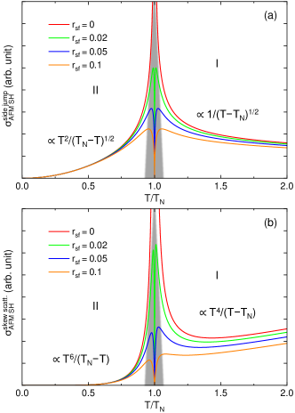
Figure 4: Schematic temperature dependence of the SH conductivity of antiferromagnets in the $T$ regimes I and II with nonzero $T_{N}$. The side-jump contribution $\sigma_{AFM,SH}^{side\,jump}$ is shown in (a) and the skew-scattering contribution $\sigma_{AFM,SH}^{skew\,scatt.}$ is shown (b). The carrier lifetime is modeled as $\tau_{\mathbf{k}}^{-1}=r_{dis}+r_{ee}T^{2}+r_{sf}T^{3}/|T-T_{N}|$, with $r_{dis}$, $r_{ee}$, and $r_{sf}$ terms representing the disorder and impurity effects, electron-electron interaction, and the AFM SF, respectively. $r_{sf}$ is varied with fixing $r_{dis}=r_{ee}=1$. Shaded areas indicate where the current treatment breaks down, requiring the self-consistent treatment.

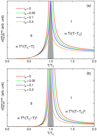
Figure 5: Schematic temperature dependence of the SH conductivity ferromagnets in the $T$ regimes I and II with nonzero $T_{C}$. The side-jump contribution $\sigma_{FM,SH}^{side\,jump}$ is shown in (a) and the skew-scattering contribution $\sigma_{FM,SH}^{skew\,scatt.}$ is shown (b). The carrier lifetime is modeled as $\tau_{\mathbf{k}}^{-1}=r_{dis}+r_{ee}T^{2}+r_{sf}T^{3}/|T-T_{C}|$, with $r_{dis}$, $r_{ee}$, and $r_{sf}$ terms representing the disorder and impurity effects, electron-electron interaction, and the AFM SF, respectively. $r_{sf}$ is varied with fixing $r_{dis}=r_{ee}=1$. Shaded areas indicate where the current treatment breaks down, requiring the self-consistent treatment.

The temperature dependence of $\sigma_{SH}$ coming from $\delta$, $\tilde{I}_{AFM}$, and $I_{AFM,FM}$ is summarized in Table 1. Reflecting the diverging behavior of $\tilde{I}_{AFM}$ and $I_{AFM,FM}$, $\sigma_{SH}$ is sharply enhanced as $T\rightarrow T_{N,C}$ in the regimes I and II, as displayed in Figures 4 for the AFM case and 5 for the FM case. Here, the approximate inverse carrier lifetime appropriate in these $T$ regime is considered as $\tau_{\mathbf{k}}^{-1}=r_{dis}+r_{ee}T^{2}+r_{sf}T^{3}/|T-T_{N,C}|$, where $r_{dis}$, $r_{ee}$, and $r_{sf}$ terms correspond to the disorder effect, electron-electron interaction [39], and the SF, respectively. Focusing on the low $T$ behavior, we ignored the electron-phonon coupling, which would contribute to the carrier lifetime at high temperatures close to the Debye temperature [40, 41]. In the current theory, there are three energy units; the Fermi energy $\varepsilon_{F}\approx\hbar v_{F}/a$, the spin stiffness $A/a^{2}$ and magnetic transition temperature $T_{N,C}$. The temperature dependence of $\sigma_{AFM,FM}^{skew\,scatt.}$ and $\sigma_{FM}^{side\,jump}$ is from $I_{AFM,FM}(T,\delta)$, and therefore $T$ is scaled by $\varepsilon_{F}$, while $\sigma_{AFM}^{sidejump}$ is from $\tilde{I}_{AFM}(T,\delta)$ and $T$ is scaled by $A/a^{2}$. For the analytical plots, we use the dimensionless unit for temperature, where $T$ is scaled by these energy units, and $T_{N,C}=1$ for the $T$ regimes I and II. With this convention, $r_{dis}$, $r_{ee}$, $r_{sf}$ have the unit of inverse time.

Despite the diverging trend as $T\rightarrow T_{N}$, $\sigma_{AFM,SH}^{side\,jump}$ and $\sigma_{AFM,SH}^{skew\,scatt.}$ sharply drop to zero in the vicinity of $T_{N}$ with nonzero $r_{sf}$. This is caused by the suppression of $\tau_{\mathbf{k}}$ due to the SF. We anticipate that a self-consistent treatment of the original model leads to a smooth $T$ dependence of $\sigma_{SH}$.

$\sigma_{FM,SH}^{side\,jump}$ and $\sigma_{FM,SH}^{skew\,scatt.}$ have stronger $T$ dependence than the AFM counterparts, leading to the divergence with $T$ approaches $T_{C}$ with $r_{sf}=0$. Nonzero $r_{sf}$ suppress the divergence in $\sigma_{FM,SH}^{side\,jump}$ and $\sigma_{FM,SH}^{skew\,scatt.}$ in the vicinity of $T_{C}$, leading to sharp cusps. However, similar to the AFM case, we anticipate that a self-consistent treatment of the original model leads to a smooth $T$ dependence of $\sigma_{SH}$ across $T_{C}$.

For the quantum critical regime III, the carrier lifetime has the temperature dependence as $\tau_{\mathbf{k}}^{-1}=r_{dis}+r_{ee}T^{2}+r_{sf}T^{3/2}$ for the AFM case and the FM with disorder effects. The temperature dependence of $\sigma_{SH}$ is strongly influenced by the temperature dependence of $\tau_{\mathbf{k}}$. Thus, here we discuss the cases with disorder effect which make $\tau_{\mathbf{k}}$ finite at $T=0$. Special cases, where the disorder effect is absent and $\tau_{\mathbf{k}}$ becomes infinity at $T=0$, will be briefly discussed in Ref. [32].

The schematic temperature dependence of $\sigma_{AFM,SH}$ and $\sigma_{FM,SH}$ is shown in Fig. 6 and 7, respectively. With nonzero $r_{dis}$, all $\sigma_{SH}$ approach 0 with $T$ goes to 0 but with different slope; $\sigma_{AFM,SH}^{side\,jump}\propto T^{3/2}$, $\sigma_{AFM,SH}^{skew\,scatt.}\propto T^{9/2}$, $\sigma_{FM,SH}^{side\,jump}\propto T^{3/2}$, and $\sigma_{FM,SH}^{skew\,scatt.}\propto T^{3}$. For the latter two cases, different power laws of $T$ were predicted in Ref. [19] as mentioned in Ref. [42].

Interestingly, $\sigma_{AFM,SH}^{side\,jump}$ and $\sigma_{FM,SH}^{side\,jump}$ show formally the same leading $T$ dependence because the divergence of the SF propagator has a cutoff by $|\mathbf{Q}|$ in the former and $q_{c}$ in the latter. On the other hand, $\sigma_{AFM,SH}^{skew\,scatt.}$ and $\sigma_{FM,SH}^{skew\,scatt.}$ show contrasting $T$ dependence; the former continuously decreases with decreasing $T$ while the latter first increases, shows maximum, and finally goes to zero with decreasing $T$ because of the competition between $\tau_{\mathbf{k}}$ and $I_{FM}(T,\delta)$.

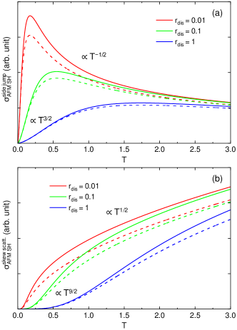
Figure 6: Schematic temperature dependence of the SH conductivity of antiferromagnets in the $T$ regime III with $T_{N}\rightarrow 0$. The side-jump contribution $\sigma_{AFM,SH}^{side\,jump}$ is shown in (a), and the skew-scattering contribution $\sigma_{AFM,SH}^{skew\,scatt.}$ shown in (b). The carrier lifetime is modeled as $\tau_{\mathbf{k}}^{-1}=r_{dis}+r_{ee}T^{2}+r_{sf}T^{3/2}$, and $r_{dis}$ is varied with fixing $r_{ee}=1$ and $r_{sf}=0.0$ $(0.1)$ for solid (dashed) lines.

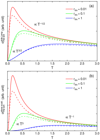
Figure 7: Schematic temperature dependence of the SH conductivity of ferromagnets in the $T$ regime III with $T_{C}\rightarrow 0$. The side-jump contribution $\sigma_{FM,SH}^{side\,jump}$ is shown in (a), and the skew-scattering contribution $\sigma_{FM,SH}^{skew\,scatt.}$ shown in (b). The carrier lifetime is modeled as $\tau_{\mathbf{k}}^{-1}=r_{dis}+r_{ee}T^{2}+r_{sf}T^{3/2}$, and $r_{dis}$ is varied with fixing $r_{ee}=1$ and $r_{sf}=0$ $(0.1)$ for solid (dashed) lines.

Discussion

Relative strength between skew scattering and side jump Now, we discuss the relative strength of the side-jump contribution and the skew-scattering contribution. When the FM critical fluctuation is dominant in the carrier lifetime in the temperature regime III, the carrier lifetime is given by $\tau_{sf}\approx\hbar/2\bigl{\{}F_{0}+2F_{1}k_{F}^{2}\bigr{\}}^{2}I_{FM}(T,\delta)$, and therefore the ratio between the maximum $\sigma_{FM,SH}^{skew\,scatt.}$ and the maximum $\sigma_{FM,SH}^{side\,jump}$ is estimated as $\sigma_{FM,SH}^{skew\,scatt.}/\sigma_{FM,SH}^{side\,jump}\approx\varepsilon_{F}{\cal F}_{3}/{\cal F}_{0}{\cal F}_{2}$ {see, Eqs. (6) and (7) and the discussion in Ref. [19]}. From the typical interaction strengths ${\cal F}$s and the Fermi energy $\varepsilon_{F}$, the maximum of $\sigma_{FM,SH}^{skew\,scatt.}$ is expected to be 1 to 2 orders of magnitude larger than that of $\sigma_{FM,SH}^{side\,jump}$. This relation is expected be hold for the FM case with finite $T_{C}$.

When disorder effects or electron-electron scattering becomes dominant in the carrier lifetime, the magnitude of $\tau_{\mathbf{k}}$ and $I_{FM}(T,\delta)$ has to be explicitly considered. Using the asymptotic form of $I_{FM}(T,\delta)$ near $\delta\sim 0$ in the $T$ regimes of I, II, and III, $I_{FM}(T,\delta)\approx\frac{1}{8\pi}(\frac{aT}{\hbar v_{F}})^{3}\frac{1}{\delta}$ (see Ref. [32]) for details) the ratio between $\sigma^{skew\,scatt.}_{FM,SH}$ and $\sigma^{side\,jump}_{FM,SH}$ is estimated as

$$\frac{\sigma^{skew\,scatt.}_{FM,SH}}{\sigma^{side\,jump}_{FM,SH}}\approx\frac{k_{F}^{2}}{4\pi m}\tau_{\mathbf{k}}{\cal F}_{0}\frac{{\cal F}_{3}}{{\cal F}_{2}}\biggl{(}\frac{aT}{\hbar v_{F}}\biggr{)}^{3}\frac{1}{\delta}.$$ (8)

Because of the factor of $1/\delta$, this ratio diverges when $\delta$ goes to zero as $T$ approaches $T_{C}$ as long as $\tau_{\mathbf{k}}$ is finite. Thus, the skew-scattering mechanism is expected to become dominant near the critical temperature. On the other hand near the FM QCP, the side-jump contribution may grow with lowering temperature when the carrier lifetime is dominated by other mechanisms than the SF.

In the AFM-fluctuation case, the situation is more complicated. This is because the side-jump contribution and the skew-scattering contribution have different temperature dependence, $\tilde{I}_{AFM}(T,\delta)$ vs. $I_{AFM}(T,\delta)$, while they show similar enhancement near the magnetic transition temperature. Therefore, the microscopic parameters determining the SF come into play. To see this, first consider the temperature regimes I and II, where the leading temperature dependence of $\sigma_{AFM,SH}^{side\,jump}$ and $\sigma_{AFM,SH}^{skew\,scatt.}$ is given by

$$\sigma_{AFM,SH}^{side\,jump}\approx\frac{e^{2}m}{32\pi^{2}\hbar^{4}}\frac{\tau_{\mathbf{k}}}{|\mathbf{Q}|}\,{\cal F}_{0}k_{F}^{2}{\cal F}_{2}\,\frac{T^{2}}{\Gamma\sqrt{\delta(A/a^{2})^{3}}}$$ (9)

and

$$\sigma_{AFM,SH}^{skew\,scatt.}\approx\frac{e^{2}}{128\pi^{3}\hbar^{3}}\frac{\tau_{\mathbf{k}}^{2}}{|\mathbf{Q}|}\,{\cal F}_{0}^{2}k_{F}^{2}{\cal F}_{3}\,\biggl{(}\frac{T}{\varepsilon_{F}}\biggr{)}^{\!\!6}\frac{\Gamma}{\delta},$$ (10)

respectively. Here, we approximate $k_{F}\approx 1/a$ (inverse lattice constant), so that $\hbar v_{F}/a\approx\varepsilon_{F}$. The ratio between these two contributions thus reads

$$\frac{\sigma_{AFM,SH}^{skew\,scatt.}}{\sigma_{AFM,SH}^{side\,jump}}\approx\frac{1}{2\pi}\frac{\tau_{\mathbf{k}}}{\hbar}\,\Gamma^{2}{\cal F}_{0}\frac{{\cal F}_{3}}{{\cal F}_{2}}\frac{T^{4}}{\varepsilon_{F}^{5}}\sqrt{\frac{(A/a^{2})^{3}}{\delta}}.$$ (11)

Thus, the relative strength depends on both electronic properties and the SF. On the electronic part, (i) longer lifetime $\tau_{\mathbf{k}}$, (ii) larger ${\cal F}_{3}$ than ${\cal F}_{2}$, and (iii) smaller Fermi energy $\varepsilon_{F}$ prefer the skew-scattering mechanism over the side jump. On the SF part, (iv) larger $A$, corresponding to spin stiffness or magnetic exchange, (v) larger damping ratio $\Gamma$, which is a dimensionless parameter here but is proportional to the electron density of states at the Fermi level, and (vi) smaller $\delta$ prefer the skew-scattering contribution.

Near the AFM QCP (the $T$ regime III), $\sigma_{SH}^{side\,jump}$ is modified as

$$\sigma_{AFM,SH}^{side\,jump}\approx\frac{e^{2}m}{2\pi^{3}\hbar^{4}}\frac{\tau_{\mathbf{k}}}{|\mathbf{Q}|}\,{\cal F}_{0}k_{F}^{2}{\cal F}_{2}\,\frac{T^{3/2}}{\Gamma\sqrt{(A/a^{2})^{3}}}$$ (12)

Hence, with $\delta=T^{3/2}$, the ratio between the two contributions becomes

$$\frac{\sigma_{AFM,SH}^{skew\,scatt.}}{\sigma_{AFM,SH}^{side\,jump}}\approx\frac{\pi}{32}\frac{\tau_{\mathbf{k}}}{\hbar}\,\Gamma^{2}{\cal F}_{0}\frac{{\cal F}_{3}}{{\cal F}_{2}}\frac{T^{3}}{\varepsilon_{F}^{5}}\sqrt{(A/a^{2})^{3}}.$$ (13)

Thus, $\sigma_{AFM,SH}^{side\,jump}$ is expected to become progressively dominant as $T\rightarrow 0$. This could be seen in the contrasting $T$ dependence of $\sigma_{AFM,SH}$ as plotted in Fig. 6.

Materials consideration In this work, we first considered the SH effect by the AFM SF, which is relevant to AFM metallic Cr. As early studies have shown, metallic Cr shows large SH effect [29, 30]. With the small SOC for a $3d$ element, this indicates additional contributions to the SH effect. Recent study used high-quality single crystal of Cr and revealed the detailed temperature dependence of the SH conductivity [31]. Their electric resistivity data does not show a strong anomaly at $T_{N}$. This indicates that the carrier lifetime is influenced by magnetic ordering and the AFM SF only weakly and, thus, the system is in the perturbative regime, corresponding to very small $r_{sf}$ in the plots of Fig. 4. Thus, the strong enhancement in the SH conductivity could be ascribed to the mechanisms developed in this work. The remaining question is which mechanism provides the main contribution to the SH effect in Cr, the side-jump mechanism or the skew-scattering mechanism. This will be answered when the SF fluctuation spectrum is carefully analyzed. Such analyses will also be helpful to understand and predict other AFM metallic systems for the SH effect.

How about AFM quantum critical fluctuation? At this moment, we are unaware of experimental reports of the SH effect in the vicinity of the AFM QCP. It might be worth investing the SH effect using CeCu_6-xAu_x [43] and other Ce compounds [44]. The temperature dependence of the SH conductivity might provide further insight into the nature of their QCP.

The SH effect near the FM critical temperature appears to depend on the material. Early studies on Ni-Pd alloys [24] reported that the temperature dependence of the SH effect is analogous to that of the uniform second-order nonlinear susceptibility $\chi_{2}$, with a positive peak above $T_{C}$ and a negative peak below $T_{C}$, thus showing the sign change across $T_{C}$. Such a behavior is qualitatively reproduced by a theoretical work by Gu et al. [27], which adopted a static mean field approximation to the Kondo’s model [28]. The current work, on the other hand, predicts that the SH effect of FM metals is maximized at $T_{C}$, while the same model is used as Gu et al.. An experimental study by Ou et al. reported the sharp enhancement of the SH effect near $T_{C}$ of Fe-Pt alloys [25], the behavior resembles our prediction. A more recent experimental study by Wu et al. also reported a similar but weaker enhancement of the SH effect of Ni-Cu alloys [26]. How the SH effect depends on the material, changing sign or maximizing at $T_{C}$, remains an open question. One possible scenario is that the spin dynamics in Ni-Pd alloys is “classical” in nature, while that in Fe-Pt and Ni-Cu alloys is more “quantum”, so that the theoretical analysis presented in this work is more relevant to the latter. Detailed experimental analysis on the spin dynamics of these FM metallic alloys using inelastic neutron scattering would settle this issue.

At this moment, it is not clear which SF generates the larger spin Hall effect, AFM or FM. It would depend on the detail of the materials property. From the leading temperature dependence, the FM SF gives a stronger temperature dependence of the spin Hall conductivity when approaching $T_{C}$ from above than the AFM fluctuation when approaching $T_{N}$. For FM metals, the spin Hall effect is expected to be replaced by the anomalous Hall effect below $T_{C}$, which is not the scope of the current study, while for AFM metals the spin Hall effect should persists down to low temperatures. Thus, both systems could be useful depending on the temperature range.

To summarize, we developed the comprehensive theoretical description of the spin Hall effect in magnetic metallic systems due to the spin fluctuation. The special focus is paid to the antiferromagnetic spin fluctuation with nonzero Néel temperature $T_{N}$ and $T_{N}=0$, and the FM SF with nonzero Curie temperature $T_{C}$. In contrast to the spin Hall effect due to the ferromagnetic critical fluctuation, where the skew-scattering mechanism is one or two orders of magnitude stronger than the side-jump mechanism, the relative strength of the mechanisms could be altered depending on the detail of the spin-fluctuation spectrum and temperature. In particular, for antiferromagnetic metals, the skew-scattering mechanism becomes progressively dominant when approaching the magnetic transition temperature $T_{N}$, while the side-jump contribution becomes dominant by lowering temperature below $T_{N}$. The crossover from the skew scattering to the side jump also appears in a quantum critical system, where $T_{N}$ is tuned to zero temperature. Aside from the absolute magnitude of the spin Hall conductivity, antiferromagnetic metals and ferromagnetic metals could be complementary in nature. This work thus provides an important component in antiferromagnetic spintronics [45].

S1 Kondo model in the momentum space

The original model, that was proposed by Kondo in Ref. [1] and adopted by the current authors in Ref. [2], has a mixed representation of momentum of conduction electrons and real-space coordinate of localized magnetic moments. This is suited to describe metallic systems, where localized magnetic moments do not necessarily form a periodic lattice. For magnetic metallic systems, wher localized magnetic moments form a periodic lattice and conduction electrons hop through the same lattice sites, it is more convenient to start from a model Hamiltonian represented in the momentum space.

The model Hamiltonian adopted in Ref. [2] is given by

$$H_{K}\!\! = \!\!-\frac{1}{N}\sum_{n}^{N_{m}}\sum_{\mathbf{k},\mathbf{k}^{\prime}}\sum_{\nu,\nu^{\prime}}e^{i(\mathbf{k}^{\prime}-\mathbf{k})\cdot\mathbf{R}_{n}}a_{\mathbf{k}\nu}^{\dagger}a_{\mathbf{k}^{\prime}\nu^{\prime}}\biggl{[}2(\mathbf{J}_{n}\cdot\mathbf{s}_{\nu\nu^{\prime}})\bigl{\{}{\cal F}_{0}+2{\cal F}_{1}(\mathbf{k}\cdot\mathbf{k}^{\prime})\bigr{\}}+i{\cal F}_{2}\mathbf{J}_{n}\cdot(\mathbf{k}^{\prime}\times\mathbf{k})$$ (S1)

$$+ \!\!i{\cal F}_{3}\Bigl{\{}(\mathbf{J}_{n}\cdot\mathbf{s}_{\nu\nu^{\prime}})\bigl{(}\mathbf{J}_{n}\cdot(\mathbf{k}^{\prime}\times\mathbf{k})\bigr{)}+\bigl{(}\mathbf{J}_{n}\cdot(\mathbf{k}^{\prime}\times\mathbf{k})\bigr{)}(\mathbf{J}_{n}\cdot\mathbf{s}_{\nu\nu^{\prime}})-\frac{2}{3}(\mathbf{J}_{n}\cdot\mathbf{J}_{n})\bigl{(}\mathbf{s}_{\nu\nu^{\prime}}\cdot(\mathbf{k}^{\prime}\times\mathbf{k})\bigr{)}\Bigr{\}}\biggr{]}.$$

Here, $a_{\mathbf{k}\nu}^{({\dagger})}$ is the annihilation (creation) operator of a conduction electron with momentum $\mathbf{k}$ and spin $\nu$, $\varepsilon_{\mathbf{k}}=\frac{\hbar^{2}k^{2}}{2m}-\varepsilon_{F}$ is the dispersion relation measured from the Fermi energy $\varepsilon_{F}$ with the carrier effective mass $m$, $\mathbf{s}_{\nu\nu^{\prime}}=\frac{1}{2}\mbox{\boldmath$\sigma$}_{\nu\nu^{\prime}}$is the conduction electron spin with the Pauli matrices $\sigma$, and $N(N_{m})$ is the total number of lattice sites (local moments). $\mathbf{J}_{n}$ is a local magnetic moment at position $\mathbf{R}_{n}$, when the SOC is weaker than the crystal field splitting and could be treated as a perturbation, or the local total angular momentum, when the SOC is strong so that the total angular momentum is a constant of motion. Parameters ${\cal F}_{l}$ are related to $F_{l}$ defined in Ref. [1] as discussed in Ref. [2].

For the current periodic system with $N_{m}=N$, we introduce the Fourier transform to localized moments as

$$\mathbf{J}_{n}=\frac{1}{\sqrt{N}}\sum_{\mathbf{p}}\mathbf{J}_{\mathbf{p}}e^{i\mathbf{p}\cdot\mathbf{R}_{n}}$$ (S2)

and the normalization $\frac{1}{N}\sum_{n}e^{i(\mathbf{k}-\mathbf{k}^{\prime})\cdot\mathbf{R}_{n}}=\delta_{\mathbf{k}\mathbf{k}^{\prime}}$. The annihilation operator of an electron $a_{\mathbf{k}\nu}$ follows the same rule.

After introducing this Fourier transform, the Hamiltonian describing the coupling between localized moments and itinerant electrons is given entirely in the momentum space as presented in Eq. (1) in the main text.

As in the conventional SH effect, a side-jump-type contribution to the SH effect arises from the anomalous velocity. Using a standard derivation $\mathbf{v}=(i/\hbar)[H_{K},\mathbf{r}]$, the velocity operator is obtained as

$$\mathbf{v}=\sum_{\mathbf{k}}\frac{\hbar\mathbf{k}}{m}a_{\mathbf{k}\nu}^{\dagger}a_{\mathbf{k}\nu}-\frac{i{\cal F}_{2}}{\hbar\sqrt{N}}\sum_{\mathbf{k},\mathbf{k}^{\prime}}\sum_{\nu,\nu^{\prime}}\mathbf{J}_{\mathbf{k}-\mathbf{k}^{\prime}}\times(\mathbf{k}^{\prime}-\mathbf{k})a_{\mathbf{k}\nu}^{\dagger}a_{\mathbf{k}^{\prime}\nu^{\prime}}.$$ (S3)

Here, we neglected terms involving ${\cal F}_{1,3}$ because these terms do not contribute to $\sigma_{SH}$ at the lowest order. The second term involving ${\cal F}_{2}$ is the anomalous velocity. The charge current and the spin current are given by using the velocity operator as $\mathbf{j}^{c}=-e\mathbf{v}$ and $\mathbf{j}^{s}=-e\{\frac{1}{N}\sum_{\mathbf{k}}s_{\nu\nu^{\prime}}^{z}a_{\mathbf{k}\nu}^{\dagger}a_{\mathbf{k}\nu^{\prime}},\mathbf{v}\}$, respectively. These current operators have the same dimension.

S2 Spin-Hall conductivity of antiferromagnets

Here, we highlight the formalism to compute the spin-Hall conductivity $\sigma_{SH}$ as described in Ref. [2]. The frequency-dependent SH conductivity is formally expressed as

$$\sigma_{SH}(i\Omega_{l})=\frac{i}{i\Omega_{l}V}\int_{0}^{1/T}d\tau e^{i\Omega_{l}\tau}\langle T_{\tau}j_{x}^{s}(\tau)j_{y}^{c}(0)\rangle.$$ (S4)

Here, $\Omega_{l}$ is the bosonic Matsubara frequency, which is analytically continued to real frequency as $i\Omega_{l}\rightarrow\Omega+i0^{+}$ at the end of the analysis, and then the DC limit, $\Omega\rightarrow 0$, is taken to obtain $\sigma_{SH}$. $V$ is the volume of the system. The imaginary time $\tau$ dependence is explicitly shown for the current operators $j_{x}^{s}(\tau)$ and $j_{y}^{c}(0)$. These current operators are defined in the main text.

Based on the diagrammatic representations in Figs. 2 and 3 in the main text, $\sigma_{SH}$ is expressed in terms of electron Green’s function $G$ and the propagator $D$ of the longitudinal spin fluctuation. Detailed analyses of the side-jump contribution $\sigma_{SH}^{side\,jump}$ and the skew-scattering contribution $\sigma_{SH}^{skew\,scatt.}$ are presented in the following subsections.

S2.1 Side jump

The SH conductivity by the side-jump mechanism as diagramatically shown in Fig. 2 is expressed in terms of the electron Green’s function and the propagator of the spin fluctuation as

$$\sigma^{side\,jump}_{AFM,SH}(i\Omega_{l})\!\!\! = \!\!\!\frac{1}{i\Omega_{l}}\frac{2e^{2}}{m}\frac{T^{2}}{VN}\sum_{l,l^{\prime}}\sum_{\mathbf{k},\mathbf{k}^{\prime}}\Bigl{\{}{\cal F}_{0}k_{x}^{2}-2{\cal F}_{1}k_{x}^{2}\bigl{(}k^{\prime}_{x}\bigr{)}^{2}\Bigr{\}}{\cal F}_{2}D_{\mathbf{k}^{\prime}-\mathbf{k}}(i\varepsilon_{l^{\prime}}-i\varepsilon_{l})$$ (S5)

$$\times \!\!\!G_{\mathbf{k}}(i\varepsilon_{l})G_{\mathbf{k}}(i\varepsilon_{l}+i\hbar\Omega_{l})\bigl{\{}G_{\mathbf{k}^{\prime}}(i\varepsilon_{l^{\prime}}+i\hbar\Omega_{l})-G_{\mathbf{k}^{\prime}}(i\varepsilon_{l^{\prime}})\bigr{\}}$$

where, $G_{\mathbf{k}}(i\varepsilon_{l})=\{i\varepsilon_{l}-\varepsilon_{\mathbf{k}}-\Sigma_{\mathbf{k}}(i\varepsilon_{l})\}^{-1}$ is the electron Matsubara Green’s function, with the fermionic Matsubara frequency $\varepsilon_{l}=(2l+1)\pi T$. The Planck constant $\hbar$ is included explicitly in front of the Matsubara frequency $\Omega_{l}$.

After carrying out the Matsubara summation, and taking the limit of $i\Omega_{l}\rightarrow 0$, one obtains

$$\sigma^{side\,jump}_{AFM,SH}\!\!\! = \!\!\!\frac{2e^{2}\hbar}{\pi mVN}\!\int\!\!d\varepsilon d\omega\sum_{\mathbf{k},\mathbf{k}^{\prime}}\Bigl{\{}{\cal F}_{0}k_{x}^{2}-2{\cal F}_{1}k_{x}^{2}\bigl{(}k^{\prime}_{x}\bigr{)}^{2}\Bigr{\}}{\cal F}_{2}B_{\mathbf{k}^{\prime}-\mathbf{k}}(\omega)\Bigl{\{}b(\omega)+f\bigl{(}\varepsilon_{\mathbf{k}^{\prime}}\bigr{)}\Bigr{\}}$$ (S6)

$$\times \!\!\!\Bigl{[}\partial_{\varepsilon}f(\varepsilon)\bigl{|}G_{\mathbf{k}}^{R}(\varepsilon)\bigr{|}^{2}\Im\bigl{\{}G_{\mathbf{k}^{\prime}}^{R}(\varepsilon+\omega)\bigr{\}}+f(\varepsilon)\Im\bigl{\{}G_{\mathbf{k}}^{R}(\varepsilon)G_{\mathbf{k}}^{R}(\varepsilon)\partial_{\varepsilon}G_{\mathbf{k}^{\prime}}^{R}(\varepsilon+\omega)\bigr{\}}\Bigr{]}.$$

$f(\varepsilon)$ and $b(\omega)$ are the Fermi distribution function and the Bose distribution function, respectively. $G_{\mathbf{k}}^{R,A}(\varepsilon)=G_{\mathbf{k}}(i\varepsilon_{l}\rightarrow\varepsilon\pm i\hbar/2\tau_{\mathbf{k}})$ are the retarded and advanced Green’s function, respectively. Here, the self-energy is assumed to be independent of $\varepsilon$, and $\tau_{\mathbf{k}}$ is the carrier lifetime. $B_{\mathbf{p}}(\omega)$ is the spectral function of the $J$ propagator given by $B_{\mathbf{p}}(\omega)=-\frac{1}{\pi}\Im D_{\mathbf{p}}(i\omega_{l}\rightarrow\omega+i0^{+})=\frac{1}{\pi}\frac{\omega/\Gamma}{\bigl{\{}\delta+A|\mathbf{p}-\mathbf{Q}|^{2}\bigr{\}}^{2}+(\omega/\Gamma)^{2}}$.

The first term in the square bracket of Eq. (S6) is proportional to $\partial_{\varepsilon}f(\varepsilon)\approx-\delta(\varepsilon)$, the so-called Fermi surface term, while the second term is proportional to $f(\varepsilon)$, the so-called Fermi sea term. In principle, two terms contribute, but it can be shown that the contribution from the second term, the Fermi sea term, is small. Thus, we focus on the first contribution.

We use the following approximations considering the small self-energy $\Sigma_{\mathbf{k}}(\varepsilon)=i\hbar/2\tau_{\mathbf{k}}$: $|G^{R}_{\mathbf{k}}(\varepsilon)|^{2}\approx(2\pi\tau_{\mathbf{k}}/\hbar)\delta(\varepsilon-\varepsilon_{\mathbf{k}})$ and $\Im G^{R}_{\mathbf{k}}(\varepsilon)\approx-\pi\delta(\varepsilon-\varepsilon_{\mathbf{k}})$. Carrying out $\varepsilon$ integral, one finds

$$\sigma^{side\,jump}_{AFM,SH}=-\frac{2e^{2}\hbar}{\pi mVN}\!\int\!\!d\omega\sum_{\mathbf{k},\mathbf{k}^{\prime}}\Bigl{\{}{\cal F}_{0}k_{x}^{2}-2{\cal F}_{1}k_{x}^{2}\bigl{(}k^{\prime}_{x}\bigr{)}^{2}\Bigr{\}}{\cal F}_{2}B_{\mathbf{k}^{\prime}-\mathbf{k}}(\omega)\bigl{\{}b(\omega)+f(\omega)\bigr{\}}\bigl{|}G_{\mathbf{k}}^{R}(0)\bigr{|}^{2}\Im\bigl{\{}G_{\mathbf{k}^{\prime}}^{R}(\omega)\bigr{\}}.$$ (S7)

For the sake of convenience, we change the momentum variable from $\mathbf{k}^{\prime}-\mathbf{k}$ to $\mathbf{q}$ and the notation from $B_{\mathbf{q}}(\omega)=\frac{1}{\pi}\frac{\omega/\Gamma}{\bigl{(}\delta+A|\mathbf{q}-\mathbf{Q}|^{2}\bigr{)}^{2}+(\omega/\Gamma)^{2}}$ to $B_{\mathbf{q}}(\omega)=\frac{1}{\pi}\frac{\omega/\Gamma}{\bigl{(}\delta+Aq^{2}\bigr{)}^{2}+(\omega/\Gamma)^{2}}$, where $\mathbf{q}$ is the momentum variable measured from magnetic wave vector $\mathbf{Q}$. Thus, Eq. (S7) is re-expressed as

$$\sigma^{side\,jump}_{AFM,SH}=-\frac{2e^{2}\hbar}{\pi mVN}\!\int\!\!d\omega\sum_{\mathbf{k},\mathbf{q}}F_{\mathbf{k},\mathbf{q}}(\omega)\bigl{|}G_{\mathbf{k}}^{R}(0)\bigr{|}^{2}\Im\bigl{\{}G_{\mathbf{k}+\mathbf{Q}+\mathbf{q}}^{R}(\omega)\bigr{\}},$$ (S8)

with $F_{\mathbf{k},\mathbf{q}}(\omega)=\Bigl{\{}{\cal F}_{0}k_{x}^{2}-2{\cal F}_{1}k_{x}^{2}\bigl{(}k_{x}+Q_{x}+q_{x}\bigr{)}^{2}\Bigr{\}}{\cal F}_{2}B_{\mathbf{q}}(\omega)\bigl{\{}b(\omega)+f(\omega)\bigr{\}}$.

Using $\bigl{|}G_{\mathbf{k}}^{R}(0)\bigr{|}^{2}=(2\pi\tau_{\mathbf{k}}/\hbar)\delta(\varepsilon_{\mathbf{k}})$ and $\Im\bigl{\{}G_{\mathbf{k}+\mathbf{Q}+\mathbf{q}}^{R}(\omega)\bigr{\}}=-\pi\delta(\omega-\varepsilon_{\mathbf{k}+\mathbf{Q}+\mathbf{q}})$ explicitly, with $\varepsilon_{\mathbf{k}+\mathbf{Q}+\mathbf{q}}=\frac{\hbar^{2}}{2m}(\mathbf{k}+\mathbf{Q}+\mathbf{q})^{2}-\varepsilon_{F}$, one proceeds to the $\mathbf{k}$ integral to find

$$\sigma^{side\,jump}_{SH}\!\!\! = \!\!\!\frac{1}{N}\frac{e^{2}k_{F}}{2\pi^{2}\hbar^{2}}\int\!\!d\omega\sum_{\mathbf{q}}\int_{0}^{2\pi}\!\!d\varphi\int_{0}^{\pi}\!\!\sin\theta d\theta\,\tau_{\mathbf{k}}\,F_{\mathbf{k},\mathbf{q}}(\omega)$$ (S9)

$$\times \!\!\!\delta\biggl{(}\omega-\frac{\hbar^{2}}{2m}\bigl{\{}2(\mathbf{k}+\mathbf{Q})\cdot\mathbf{q}+|\mathbf{Q}|^{2}+|\mathbf{q}|^{2}+2\cos\theta k_{F}|\mathbf{Q}|\bigr{\}}\biggr{)}\biggl{|}_{|\mathbf{k}|=k_{F}}\,$$

where $\varphi$ is the azimuth angle and $\theta$ is the polar angle of $\mathbf{k}$ measured from the $\mathbf{Q}$ direction. Here, the $\mathbf{k}$ dependence is kept in the $\delta$ function, but the size of $\mathbf{k}$ is constrained as $|\mathbf{k}|=k_{F}=\sqrt{2m\varepsilon_{F}}/\hbar$. By further carrying out the $\theta$ integral, one arrives at

$$\sigma^{side\,jump}_{AFM,SH}\!\!\! = \!\!\!\frac{1}{N}\frac{e^{2}mk_{F}}{2\pi^{2}\hbar^{4}|\mathbf{Q}|}\int\!\!d\omega\sum_{\mathbf{q}}\int_{0}^{2\pi}\!\!d\varphi\,\,\tau_{\mathbf{k}}F_{\mathbf{k},\mathbf{q}}(\omega)\Bigl{|}^{|\mathbf{k}|=k_{F}}_{\cos\theta=\frac{m}{\hbar^{2}k_{F}|\mathbf{Q}|}\Bigl{[}\omega-\frac{\hbar^{2}}{2m}\bigl{\{}2(\mathbf{k}+\mathbf{Q})\cdot\mathbf{q}+|\mathbf{Q}|^{2}+|\mathbf{q}|^{2}\bigr{\}}\Bigr{]}},$$ (S10)

where we assumed that $|\mathbf{Q}|<2k_{F}$.

Now we consider low temperature $T$ regime, where only small frequency $\omega$ and small momentum $|\mathbf{q}|$ contribute to this integral. In this case, the constraint $\cos\theta=\frac{m}{\hbar^{2}k_{F}|\mathbf{Q}|}\Bigl{[}\omega-\frac{\hbar^{2}}{2m}\bigl{\{}2(\mathbf{k}+\mathbf{Q})\cdot\mathbf{q}+|\mathbf{Q}|^{2}+|\mathbf{q}|^{2}\bigr{\}}\Bigr{]}$ can be approximated as $\cos\theta\approx-|\mathbf{Q}|/2k_{F}$ because contributions coming from $\omega$ and $\mathbf{q}$ are expected to induce only small corrections in $\sigma^{side\,jump}_{SH}$ higher-order in $T$. Together with $|\mathbf{k}|=k_{F}$, the condition $\cos\theta\approx-|\mathbf{Q}|/2k_{F}$ means that the main contribution to $\sigma^{side\,jump}_{SH}$ comes from the momenta that satisfy the nesting condition. Further, $q_{x}$ in ${\cal F}_{0}k_{x}^{2}-2{\cal F}_{1}k_{x}^{2}\bigl{(}k_{x}+Q_{x}+q_{x}\bigr{)}^{2}$ gives only small contributions to the spin-Hall conductivity. Thus, assuming that the angle dependence of $\tau_{\mathbf{k}}$ is weak, the leading term of $\sigma^{side\,jump}_{SH}$ is summarized as

$$\sigma^{side\,jump}_{AFM,SH}=\frac{e^{2}m\tau_{\mathbf{k}}}{2\pi^{2}\hbar^{4}|\mathbf{Q}|}\,A_{AFM}^{side\,jump}\,\tilde{I}_{AFM}(T,\delta),$$ (S11)

where

$$A_{AFM}^{side\,jump}=\int_{0}^{2\pi}\!\!d\varphi\bigl{\{}{\cal F}_{0}k_{x}^{2}-2{\cal F}_{1}k_{x}^{2}(k_{x}+Q_{x})^{2}\bigr{\}}{\cal F}_{2}\bigl{|}^{|\mathbf{k}|=k_{F}}_{\cos\theta=-|\mathbf{Q}|/2k_{F}},$$ (S12)

and

$$\tilde{I}_{AFM}(T,\delta)\!\!\! = \!\!\!\frac{\pi}{N}\sum_{\mathbf{q}}\int\!\!d\omega\,B_{\mathbf{q}}(\omega)\,\bigl{\{}b(\omega)+f(\omega)\bigr{\}}$$ (S13)

$$= \!\!\!\frac{a^{3}}{8\pi^{2}}\int\!\!d\omega\!\!\int\!\!d^{3}\mathbf{q}\,\frac{\omega/\Gamma}{\bigl{(}\delta+Aq^{2}\bigr{)}^{2}+(\omega/\Gamma)^{2}}\,\frac{1}{\sinh(\omega/T)}.$$

S2.2 Skew scattering

Using Matsubara Green’s functions for conduction electrons and the spin fluctuation propagator, the SH conductivity due to the skew scattering is expressed as

$$\sigma^{skew\,scat.}_{AFM,SH}(i\Omega_{l})\!\!\! = \!\!\!\frac{1}{i\Omega_{l}}\frac{e^{2}\hbar^{2}}{m^{2}}\frac{T^{3}}{VN^{2}}\sum_{l,l^{\prime},l^{\prime\prime}}\sum_{\mathbf{k},\mathbf{k}^{\prime},\mathbf{k}^{\prime\prime}}$$ (S14)

$$\times \!\!\!G_{\mathbf{k}}(i\varepsilon_{l})G_{\mathbf{k}}(i\varepsilon_{l}+i\hbar\Omega_{l})G_{\mathbf{k}^{\prime}}(i\varepsilon_{l^{\prime}})G_{\mathbf{k}^{\prime}}(i\varepsilon_{l^{\prime}}+i\hbar\Omega_{l})\bigl{\{}G_{\mathbf{k}^{\prime\prime}}(i\varepsilon_{l^{\prime\prime}}+i\hbar\Omega_{l})-G_{\mathbf{k}^{\prime\prime}}(i\varepsilon_{l^{\prime\prime}})\bigr{\}}$$

$$\times \!\!\!\Bigl{\{}-D_{\mathbf{k}-\mathbf{k}^{\prime\prime}}(i\varepsilon_{l}-i\varepsilon_{l^{\prime\prime}})D_{\mathbf{k}^{\prime}-\mathbf{k}^{\prime\prime}}(i\varepsilon_{l^{\prime}}-i\varepsilon_{l^{\prime\prime}}){\cal F}_{3}k_{x}^{2}{k^{\prime}_{y}}^{2}\bigl{(}{\cal F}_{0}+{\cal F}_{1}\mathbf{k}\cdot\mathbf{k}^{\prime\prime}\bigr{)}\bigl{(}{\cal F}_{0}+{\cal F}_{1}\mathbf{k}^{\prime}\cdot\mathbf{k}^{\prime\prime}\bigr{)}$$

$$+ \!\!\!2D_{\mathbf{k}-\mathbf{k}^{\prime}}(i\varepsilon_{l}-i\varepsilon_{l^{\prime}})D_{\mathbf{k}^{\prime\prime}-\mathbf{k}^{\prime}}(i\varepsilon_{l^{\prime\prime}}-i\varepsilon_{l^{\prime}}){\cal F}_{3}k_{x}^{2}{k^{\prime\prime}_{y}}{k^{\prime}_{y}}\bigl{(}{\cal F}_{0}+{\cal F}_{1}\mathbf{k}\cdot\mathbf{k}^{\prime}\bigr{)}\bigl{(}{\cal F}_{0}+{\cal F}_{1}\mathbf{k}^{\prime}\cdot\mathbf{k}^{\prime\prime}\bigr{)}\Bigr{\}}.$$

Here, the last term in Eq. (1) is not considered because this term is proportional to $(\mathbf{J}_{n}\cdot\mathbf{J}_{n})\approx const.$. The Matsubara summation can be carried out similarly as in the side-jump mechanism. Focusing on the Fermi surface terms, one finds

$$\sigma^{skew\,scat.}_{AFM,SH}\!\!\! = \!\!\!\frac{e^{2}\hbar^{3}}{\pi m^{2}VN^{2}}\!\int\!\!d\varepsilon d\omega d\omega^{\prime}\!\!\sum_{\mathbf{k},\mathbf{k}^{\prime},\mathbf{k}^{\prime\prime}}$$ (S15)

$$\times \!\!\!\biggl{[}{\cal F}_{3}k_{x}^{2}{k^{\prime}_{y}}^{2}\bigl{(}{\cal F}_{0}+{\cal F}_{1}\mathbf{k}\cdot\mathbf{k}^{\prime\prime}\bigr{)}\bigl{(}{\cal F}_{0}+{\cal F}_{1}\mathbf{k}^{\prime}\cdot\mathbf{k}^{\prime\prime}\bigr{)}B_{\mathbf{k}-\mathbf{k}^{\prime\prime}}(\omega)\Bigl{\{}b(\omega)+f\bigl{(}\varepsilon_{\mathbf{k}}\bigr{)}\Bigr{\}}B_{\mathbf{k}^{\prime}-\mathbf{k}^{\prime\prime}}(\omega^{\prime})\Bigl{\{}b(\omega^{\prime})+f\bigl{(}\varepsilon_{\mathbf{k}^{\prime}}\bigr{)}\Bigr{\}}$$

$$\times \!\!\!\partial_{\varepsilon}f(\varepsilon)\bigl{|}G_{\mathbf{k}}^{R}(\varepsilon+\omega)\bigr{|}^{2}\bigl{|}G_{\mathbf{k}^{\prime}}^{R}(\varepsilon+\omega^{\prime})\bigr{|}^{2}\Im\bigl{\{}G_{\mathbf{k}^{\prime\prime}}^{R}(\varepsilon)\bigr{\}}$$

$$- \!\!\!2{\cal F}_{3}k_{x}^{2}{k^{\prime\prime}_{y}}{k^{\prime}_{y}}\bigl{(}{\cal F}_{0}+{\cal F}_{1}\mathbf{k}\cdot\mathbf{k}^{\prime}\bigr{)}\bigl{(}{\cal F}_{0}+{\cal F}_{1}\mathbf{k}^{\prime}\cdot\mathbf{k}^{\prime\prime}\bigr{)}B_{\mathbf{k}-\mathbf{k}^{\prime}}(\omega)\Bigl{\{}b(\omega)+f\bigl{(}\varepsilon_{\mathbf{k}}\bigr{)}\Bigr{\}}B_{\mathbf{k}^{\prime\prime}-\mathbf{k}^{\prime}}(\omega^{\prime})\Bigl{\{}b(\omega^{\prime})+f\bigl{(}\varepsilon_{\mathbf{k}^{\prime\prime}}\bigr{)}\Bigr{\}}$$

$$\times \!\!\!\partial_{\varepsilon}f(\varepsilon)\bigl{|}G_{\mathbf{k}}^{R}(\varepsilon+\omega)\bigr{|}^{2}\bigl{|}G_{\mathbf{k}^{\prime}}^{R}(\varepsilon)\bigr{|}^{2}\Im\bigl{\{}G_{\mathbf{k}^{\prime\prime}}^{R}(\varepsilon+\omega^{\prime})\bigr{\}}\biggr{]}.$$

Again, we change momentum variables from $\mathbf{k}-\mathbf{k}^{\prime\prime}$ to $\mathbf{q}$ and from $\mathbf{k}^{\prime}-\mathbf{k}^{\prime\prime}$ to $\mathbf{q}^{\prime}$ and measure them from the magnetic wave vector $\mathbf{Q}$, and use the new notation of the spin fluctuation propagator $B$. Replacing Green’s function by $\delta$ functions and carrying out the $\varepsilon$ integral, one finds

$$\sigma^{skew\,scat.}_{AFM,SH}\!\!\! = \!\!\!\frac{4\pi^{2}e^{2}\hbar}{m^{2}VN^{2}}\!\int\!\!d\omega d\omega^{\prime}\!\!\sum_{\mathbf{k},\mathbf{q},\mathbf{q}^{\prime}}\delta\bigl{(}\varepsilon_{\mathbf{k}}\bigr{)}\delta\bigl{(}\omega-\varepsilon_{\mathbf{k}+\mathbf{Q}+\mathbf{q}}\bigr{)}\delta\bigl{(}\omega^{\prime}-\varepsilon_{\mathbf{k}+\mathbf{Q}+\mathbf{q}^{\prime}}\bigr{)}$$ (S16)

$$\times \!\!\!F_{\mathbf{k},\mathbf{q},\mathbf{q}^{\prime}}B_{\mathbf{q}}(\omega)\bigl{\{}b(\omega)+f(\omega)\bigr{\}}B_{\mathbf{q}^{\prime}}(\omega^{\prime})\bigl{\{}b(\omega^{\prime})+f(\omega^{\prime})\bigr{\}},$$

where

$$F_{\mathbf{k},\mathbf{q},\mathbf{q}^{\prime}}\!\!\! = \!\!\!{\cal F}_{3}\bigl{(}k_{x}+Q_{x}+q_{x}\bigr{)}^{2}\bigl{(}k_{y}+Q_{y}+q_{y}\bigr{)}^{2}\bigl{\{}{\cal F}_{0}+{\cal F}_{1}\mathbf{k}\cdot(\mathbf{k}+\mathbf{Q}+\mathbf{q})\bigr{\}}\bigl{\{}{\cal F}_{0}+{\cal F}_{1}\mathbf{k}\cdot(\mathbf{k}+\mathbf{Q}+\mathbf{q}^{\prime})\bigr{\}}\tau_{\mathbf{k}+\mathbf{Q}+\mathbf{q}}\,\tau_{\mathbf{k}+\mathbf{Q}+\mathbf{q}^{\prime}}$$

$$- \!\!\!2{\cal F}_{3}\bigl{(}k_{x}+Q_{x}+q_{x}\bigr{)}^{2}\bigl{(}k_{y}+Q_{y}+q_{y}\bigr{)}{k_{y}}\bigl{\{}{\cal F}_{0}+{\cal F}_{1}\mathbf{k}\cdot(\mathbf{k}+\mathbf{Q}+\mathbf{q})\bigr{\}}\bigl{\{}{\cal F}_{0}+{\cal F}_{1}\mathbf{k}\cdot(\mathbf{k}+\mathbf{Q}+\mathbf{q}^{\prime})\bigr{\}}\tau_{\mathbf{k}}\,\tau_{\mathbf{k}+\mathbf{Q}+\mathbf{q}}.$$

Carrying out polar and radial parts of the $\mathbf{k}$ integral and $\omega^{\prime}$ integral, one finds

$$\sigma^{skew\,scat.}_{AFM,SH}\!\!\! = \!\!\!\frac{1}{N^{2}}\frac{e^{2}}{2\pi\hbar^{3}|\mathbf{Q}|}\!\int\!\!d\omega d\omega^{\prime}\sum_{\mathbf{q},\mathbf{q}^{\prime}}\int_{0}^{2\pi}\!\!d\varphi\delta\bigl{(}\omega-\varepsilon_{\mathbf{k}+\mathbf{Q}+\mathbf{q}}-\omega^{\prime}+\varepsilon_{\mathbf{k}+\mathbf{Q}+\mathbf{q}^{\prime}}\bigr{)}F_{\mathbf{k},\mathbf{q},\mathbf{q}^{\prime}}$$

$$\times \!\!\!B_{\mathbf{q}}(\omega)\bigl{\{}b(\omega)+f(\omega)\bigr{\}}B_{\mathbf{q}^{\prime}}(\omega^{\prime})\bigl{\{}b(\omega^{\prime})+f(\omega^{\prime})\bigr{\}}\Bigl{|}^{|\mathbf{k}|=k_{F}}_{\cos\theta=-|\mathbf{Q}|/2k_{F}}$$

$$= \!\!\!\frac{1}{N^{2}}\frac{e^{2}}{2\pi\hbar^{3}|\mathbf{Q}|}\!\int\!\!d\omega\sum_{\mathbf{q},\mathbf{q}^{\prime}}\int_{0}^{2\pi}\!\!d\varphi\,F_{\mathbf{k},\mathbf{q},\mathbf{q}^{\prime}}\,B_{\mathbf{q}}(\omega)\bigl{\{}b(\omega)+f(\omega)\bigr{\}}$$

$$\times \!\!\!B_{\mathbf{q}^{\prime}}(\omega-\varepsilon_{\mathbf{k}+\mathbf{Q}+\mathbf{q}}+\varepsilon_{\mathbf{k}+\mathbf{Q}+\mathbf{q}^{\prime}})\bigl{\{}b(\omega-\varepsilon_{\mathbf{k}+\mathbf{Q}+\mathbf{q}}+\varepsilon_{\mathbf{k}+\mathbf{Q}+\mathbf{q}^{\prime}})+f(\omega-\varepsilon_{\mathbf{k}+\mathbf{Q}+\mathbf{q}}+\varepsilon_{\mathbf{k}+\mathbf{Q}+\mathbf{q}^{\prime}})\bigr{\}}\Bigl{|}^{|\mathbf{k}|=k_{F}}_{\cos\theta=-|\mathbf{Q}|/2k_{F}}$$

As in the side jump case, we consider low temperatures $T$, where only small $\mathbf{q}$ and $\mathbf{q}^{\prime}$ contribute to $\sigma^{skew\,scat.}_{SH}$. With the constraints $|\mathbf{k}|=k_{F}$ and $\cos\theta=-|\mathbf{Q}|/2k_{F}$, one can approximate $\varepsilon_{\mathbf{k}+\mathbf{Q}+\mathbf{q}}$ as $\varepsilon_{\mathbf{k}+\mathbf{Q}+\mathbf{q}}=\frac{\hbar^{2}}{2m}|\mathbf{k}+\mathbf{Q}+\mathbf{q}|^{2}-\varepsilon_{F}\approx\hbar\mathbf{v}_{F}\cdot\mathbf{q}$, where $\mathbf{v}_{F}=\hbar(\mathbf{k}+\mathbf{Q})/m$ is the Fermi velocity at $\mathbf{k}+\mathbf{Q}$.

Now, we re-write $B_{\mathbf{q}^{\prime}}(\omega-\varepsilon_{\mathbf{k}+\mathbf{Q}+\mathbf{q}}+\varepsilon_{\mathbf{k}+\mathbf{Q}+\mathbf{q}^{\prime}})$. In the critical regime, $|\mathbf{q}|^{2}$ and $\mathbf{\varepsilon}_{\mathbf{k}+\mathbf{Q}+\mathbf{q}^{\prime}}=\hbar\mathbf{v}_{F}\cdot\mathbf{q}^{\prime}$ are small. Under this assumption, $B_{\mathbf{q}^{\prime}}(\omega-\varepsilon_{\mathbf{k}+\mathbf{Q}+\mathbf{q}}+\varepsilon_{\mathbf{k}+\mathbf{Q}+\mathbf{q}^{\prime}})$ is re-written as follows:

$$B_{\mathbf{q}^{\prime}}(\omega-\varepsilon_{\mathbf{k}+\mathbf{Q}+\mathbf{q}}+\varepsilon_{\mathbf{k}+\mathbf{Q}+\mathbf{q}^{\prime}})\!\!\! = \!\!\!\frac{1}{\pi}\frac{(\omega-\varepsilon_{\mathbf{k}+\mathbf{Q}+\mathbf{q}}+\varepsilon_{\mathbf{k}+\mathbf{Q}+\mathbf{q}^{\prime}})/\Gamma}{\bigl{(}\delta+Aq^{\prime 2}\bigr{)}^{2}+\bigl{\{}\bigl{(}\omega-\varepsilon_{\mathbf{k}+\mathbf{Q}+\mathbf{q}}+\varepsilon_{\mathbf{k}+\mathbf{Q}+\mathbf{q}^{\prime}}\bigr{)}/\Gamma\bigr{\}}^{2}}$$ (S19)

$$\approx \!\!\!\frac{1}{\pi}\frac{\bigl{(}\omega-\varepsilon_{\mathbf{k}+\mathbf{Q}+\mathbf{q}}+\varepsilon_{\mathbf{k}+\mathbf{Q}+\mathbf{q}^{\prime}}\bigr{)}/\Gamma}{\bigl{(}\delta+Aq^{\prime 2}\bigr{)}^{2}+\bigl{\{}\bigl{(}\varepsilon_{\mathbf{k}+\mathbf{Q}+\mathbf{q}^{\prime}}\bigr{)}/\Gamma\bigr{\}}^{2}}\frac{1}{1+\frac{\bigl{\{}\bigl{(}\omega-\varepsilon_{\mathbf{k}+\mathbf{Q}+\mathbf{q}}\bigr{)}/\Gamma\bigr{\}}^{2}}{\bigl{(}\delta+Aq^{\prime 2}\bigr{)}^{2}+\bigl{\{}\bigl{(}\varepsilon_{\mathbf{k}+\mathbf{Q}+\mathbf{q}^{\prime}}\bigr{)}/\Gamma\bigr{\}}^{2}}}$$

$$\approx \!\!\!\frac{1}{\pi}\frac{\bigl{(}\omega-\varepsilon_{\mathbf{k}+\mathbf{Q}+\mathbf{q}}+\varepsilon_{\mathbf{k}+\mathbf{Q}+\mathbf{q}^{\prime}}\bigr{)}/\Gamma}{\bigl{(}\delta+Aq^{\prime 2}\bigr{)}^{2}+\bigl{\{}\bigl{(}\varepsilon_{\mathbf{k}+\mathbf{Q}+\mathbf{q}^{\prime}}\bigr{)}/\Gamma\bigr{\}}^{2}}\frac{\bigl{(}\delta+Aq^{\prime 2}\bigr{)}^{2}\,\Gamma^{2}+\varepsilon_{\mathbf{k}+\mathbf{Q}+\mathbf{q}^{\prime}}^{2}}{\bigl{(}\delta+Aq^{\prime 2}\bigr{)}^{2}\,\Gamma^{2}+\varepsilon_{\mathbf{k}+\mathbf{Q}+\mathbf{q}^{\prime}}^{2}+\bigl{(}\omega-\varepsilon_{\mathbf{k}+\mathbf{Q}+\mathbf{q}}\bigr{)}^{2}}$$

$$\approx \!\!\!\frac{1}{\pi}\frac{\bigl{(}\varepsilon_{\mathbf{k}+\mathbf{Q}+\mathbf{q}^{\prime}}\bigr{)}/\Gamma}{\bigl{(}\delta+Aq^{\prime 2}\bigr{)}^{2}+\bigl{\{}\bigl{(}\varepsilon_{\mathbf{k}+\mathbf{Q}+\mathbf{q}^{\prime}}\bigr{)}/\Gamma\bigr{\}}^{2}}\,\delta\bigl{(}\omega-\varepsilon_{\mathbf{k}+\mathbf{Q}+\mathbf{q}}\bigr{)}\,\pi\Gamma\delta$$

In the second line, a small cross term $\varepsilon_{\mathbf{k}+\mathbf{Q}+\mathbf{q}}(\omega-\varepsilon_{\mathbf{k}+\mathbf{Q}+\mathbf{q}^{\prime}})$ is neglected, and in the last line small terms $(2\delta Aq^{\prime 2}+A^{2}q^{\prime 4})\Gamma^{2}+\varepsilon_{\mathbf{k}+\mathbf{Q}+\mathbf{q}^{\prime}}^{2}$, which are proportional to $q^{\prime 2}$, are neglected and $\Gamma\delta$ is assumed to be small. Thus, at low temperatures and near the critical regime, $B_{\mathbf{q}^{\prime}}(\omega-\varepsilon_{\mathbf{k}+\mathbf{Q}+\mathbf{q}}+\varepsilon_{\mathbf{k}+\mathbf{Q}+\mathbf{q}^{\prime}})$ is approximated as

$$B_{\mathbf{q}^{\prime}}(\omega-\varepsilon_{\mathbf{k}+\mathbf{Q}+\mathbf{q}}+\varepsilon_{\mathbf{k}+\mathbf{Q}+\mathbf{q}^{\prime}})\approx B_{\mathbf{q}^{\prime}}(\varepsilon_{\mathbf{k}+\mathbf{Q}+\mathbf{q}^{\prime}})\delta\bigl{(}\omega-\varepsilon_{\mathbf{k}+\mathbf{Q}+\mathbf{q}}\bigr{)}\,\pi\Gamma\delta.$$ (S20)

Note that this approximation cannot be used to describe the behavior precisely at the critical point at finite temperature because $B_{\mathbf{q}^{\prime}}(\omega-\varepsilon_{\mathbf{k}+\mathbf{Q}+\mathbf{q}}+\varepsilon_{\mathbf{k}+\mathbf{Q}+\mathbf{q}^{\prime}})$ becomes zero as $\delta\rightarrow 0$, while $B_{\mathbf{q}^{\prime}}(\omega-\varepsilon_{\mathbf{k}+\mathbf{Q}+\mathbf{q}}+\varepsilon_{\mathbf{k}+\mathbf{Q}+\mathbf{q}^{\prime}})$ is expected to remain nonzero.

With this approximation and neglecting small contributions in $F_{\mathbf{k},\mathbf{q},\mathbf{q}^{\prime}}$ from $\mathbf{q}$ and $\mathbf{q}^{\prime}$, $\mathbf{q}$ and $\mathbf{q}^{\prime}$ integrals can be carried out separately. As a result, the leading contribution to $\sigma^{skew\,scat.}_{SH}$ is given by

$$\sigma^{skew\,scat.}_{AFM,SH}\!\!\! = \!\!\!\frac{1}{N^{2}}\frac{e^{2}}{2\pi\hbar^{3}|\mathbf{Q}|}\sum_{\mathbf{q},\mathbf{q}^{\prime}}\int_{0}^{2\pi}\!\!d\varphi F_{\mathbf{k},\mathbf{q}=0,\mathbf{q}^{\prime}=0}\,B_{\mathbf{q}}(\varepsilon_{\mathbf{k}+\mathbf{Q}+\mathbf{q}})\bigl{\{}b(\varepsilon_{\mathbf{k}+\mathbf{Q}+\mathbf{q}})+f(\varepsilon_{\mathbf{k}+\mathbf{Q}+\mathbf{q}})\bigr{\}}$$

$$\times \!\!\!B_{\mathbf{q}^{\prime}}(\varepsilon_{\mathbf{k}+\mathbf{Q}+\mathbf{q}^{\prime}})\bigl{\{}b(\varepsilon_{\mathbf{k}+\mathbf{Q}+\mathbf{q}^{\prime}})+f(\varepsilon_{\mathbf{k}+\mathbf{Q}+\mathbf{q}^{\prime}})\bigr{\}}\Bigl{|}^{|\mathbf{k}|=k_{F}}_{\cos\theta=-|\mathbf{Q}|/2k_{F}}.$$

Considering the constraints $|\mathbf{k}|=k_{F}$ and $\cos\theta=-|\mathbf{Q}|/2k_{F}$ and carrying out momentum integrals separately, one arrives at

$$\sigma^{skew\,scat.}_{AFM,SH}\!\!\! = \!\!\!\frac{e^{2}\tau_{\mathbf{k}}^{2}\,\Gamma\,\delta}{2\pi^{2}\hbar^{3}|\mathbf{Q}|}A_{AFM}^{skew\,scatt.}\,I_{AFM}^{2}(T,\delta),$$ (S22)

where $A^{skew\,scatt.}$ and $I_{AFM}(T,\delta)$ are given by

$$A_{AFM}^{skew\,scatt.}\!\!\! = \!\!\!\int_{0}^{2\pi}\!\!d\varphi\Bigl{[}{\cal F}_{3}\bigl{(}k_{x}+Q_{x}\bigr{)}^{2}\bigl{(}k_{y}+Q_{y}\bigr{)}^{2}\bigl{\{}{\cal F}_{0}+{\cal F}_{1}\mathbf{k}\cdot(\mathbf{k}+\mathbf{Q})\bigr{\}}\bigl{\{}{\cal F}_{0}+{\cal F}_{1}\mathbf{k}\cdot(\mathbf{k}+\mathbf{Q}^{\prime})\bigr{\}}$$ (S23)

$$- \!\!\!2{\cal F}_{3}\bigl{(}k_{x}+Q_{x}\bigr{)}^{2}\bigl{(}k_{y}+Q_{y}\bigr{)}{k_{y}}\bigl{\{}{\cal F}_{0}+{\cal F}_{1}\mathbf{k}\cdot(\mathbf{k}+\mathbf{Q})\bigr{\}}\bigl{\{}{\cal F}_{0}+{\cal F}_{1}\mathbf{k}\cdot(\mathbf{k}+\mathbf{Q})\bigr{\}}\Bigr{]}\Bigl{|}^{|\mathbf{k}|=k_{F}}_{\cos\theta=-|\mathbf{Q}|/2k_{F}}$$

and

$$I_{AFM}(T,\delta)\!\!\! = \!\!\!\frac{\pi}{N}\sum_{\mathbf{q}}B_{\mathbf{q}}(\hbar\mathbf{v}_{F}\cdot\mathbf{q})\bigl{\{}b(\hbar\mathbf{v}_{F}\cdot\mathbf{q})+r(\hbar\mathbf{v}_{F}\cdot\mathbf{q})\bigr{\}}$$ (S24)

$$= \frac{a^{3}}{8\pi^{2}}\!\!\!\int d^{3}\mathbf{q}\frac{\hbar\mathbf{v}_{F}\cdot\mathbf{q}/\Gamma}{\bigl{(}\delta+Aq^{2}\bigr{)}^{2}+\bigl{(}\hbar\mathbf{v}_{F}\cdot\mathbf{q}/\Gamma\bigr{)}^{2}}\frac{1}{\sinh\bigl{(}\hbar\mathbf{v}_{F}\cdot\mathbf{q}/T\bigr{)}},$$

respectively.

S2.3 Detail of $\tilde{I}_{AFM}(T,\delta)$

In this subsection, we describe the detailed behavior of $\tilde{I}_{AFM}(T,\delta)$ and their analytic forms where these are available. These results and other functions are summarized in Table SII.

Carrying out the azimuth and polar integral of $\mathbf{q}$ of Eq. (S13), $\tilde{I}_{AFM}(T,\delta)$ becomes

$$\tilde{I}_{AFM}(T,\delta)=\frac{a^{3}}{2\pi^{2}}\int\!\!d\omega\!\!\int\!\!dq\,\frac{q^{2}\omega/\Gamma}{\bigl{(}\delta+Aq^{2}\bigr{)}^{2}+(\omega/\Gamma)^{2}}\,\frac{1}{\sinh(\omega/T)}.$$ (S25)

(1) Disordered regime or ordered phase away from the finite-temperature phase transition, so that $|\delta|\gg T/\Gamma$.

This include $T$ regimes I at $T>T_{N}$ and II at $T<T_{N}$ with nonzero $T_{N}$. In this regime, the damping term $\omega/\Gamma$ can be neglected compared with $\delta$, so that

$$\tilde{I}_{AFM}(T,\delta)\approx\frac{a^{3}}{2\pi^{2}}\int_{-\infty}^{\infty}\!\!d\omega\!\!\int_{0}^{\infty}\!\!dq\,\frac{q^{2}\omega/\Gamma}{\bigl{(}\delta+Aq^{2}\bigr{)}^{2}}\,\frac{1}{\sinh(\omega/T)}.$$ (S26)

Making use of $\int_{0}^{\infty}dx\frac{x}{\sinh\,x}=\frac{\pi^{2}}{4}$, one finds

$$\tilde{I}_{AFM}(T,\delta)\approx\frac{a^{3}T^{2}}{4\Gamma}\int_{0}^{\infty}\!\!dq\,\frac{q^{2}}{\bigl{(}\delta+Aq^{2}\bigr{)}^{2}}=\frac{a^{3}T^{2}}{4\Gamma}\frac{1}{2A\sqrt{A\delta}}\arctan\frac{q}{\sqrt{A\delta}}\biggr{]}_{0}^{\infty}=\frac{\pi a^{3}T^{2}}{16\Gamma A\sqrt{A\delta}}.$$ (S27)

(2) Near the finite-temperature phase transition, so that $|\delta|\ll T/\Gamma$.

In this regime, $\delta$ can be neglected in the frequency regime at $\omega/\Gamma\gg\delta$. Considering small but not too small temperature $T$, we approximate $\frac{\omega}{\sinh(\omega/T)}$ as $\frac{\omega}{\sinh(\omega/T)}\approx T$. Then, we introduce the upper limit of the frequency integral as $T$, divide the frequency range at $\omega=\Gamma\delta$, and set $\delta=0$ above $\omega=\Gamma\delta$.

$$\tilde{I}_{AFM}(T,\delta)\!\! \approx \!\!\frac{a^{3}T}{\pi^{2}\Gamma}\int_{0}^{\infty}dq\,q^{2}\biggl{[}\int_{0}^{\delta\Gamma}d\omega\frac{1}{(\delta+Aq^{2})^{2}+(\omega/\Gamma)^{2}}+\int_{\delta\Gamma}^{T}d\omega\frac{1}{(Aq^{2})^{2}+(\omega/\Gamma)^{2}}\biggr{]}$$ (S28)

$$= \!\!\frac{a^{3}T}{\pi^{2}}\int_{0}^{\infty}dq\,q^{2}\biggl{[}\frac{1}{\delta+Aq^{2}}\arctan\frac{\delta}{\delta+Aq^{2}}+\frac{1}{Aq^{2}}\biggl{(}\arctan\frac{T}{Aq^{2}\Gamma}-\arctan\frac{\delta}{Aq^{2}}\biggr{)}\biggr{]}$$

$$= \!\!\frac{a^{3}T}{\pi^{2}}\int_{0}^{\infty}dq\,q^{2}\frac{1}{\delta+Aq^{2}}\arctan\frac{\delta}{\delta+Aq^{2}}+\frac{T}{\sqrt{2A^{3}}}\biggl{(}\sqrt{\frac{T}{\Gamma}}-\sqrt{\delta}\biggr{)}.$$

In the last line, we made use of

$$\int_{0}^{\infty}\!\!dx\arctan\frac{a}{x^{2}}=x\arctan\frac{a}{x^{2}}\biggr{]}_{0}^{\infty}+\int_{0}^{\infty}\!\!dx\frac{2ax^{2}}{x^{4}+a^{2}}=\pi\sqrt{\frac{a}{2}}.$$ (S29)

Since we are focusing at small $|\delta|$, approximating $\arctan\frac{\delta}{\delta+Aq^{2}}$ as $\arctan\frac{\delta}{\delta+Aq^{2}}\approx\frac{\delta}{\delta+Aq^{2}}$ and $\int_{0}^{\infty}dq\frac{a^{2}}{(\delta+Aq^{2})^{2}}=\frac{\pi}{4\sqrt{A^{3}\delta}}$, we arrive at

$$\tilde{I}_{AFM}(T,\delta)\approx\frac{a^{3}T}{\pi\sqrt{2A^{3}}}\biggl{[}\sqrt{\frac{T}{\Gamma}}-\biggl{(}1-\frac{1}{2\sqrt{2}}\biggr{)}\sqrt{\delta}\biggr{]}.$$ (S30)

(3) Quantum critical regime.

This corresponds to $T$ regime III. In this regime, one expects $\delta\propto T^{3/2}\ll T$. Therefore, the first term of Eq. (S30) becomes dominant. Therefore,

$$\tilde{I}_{AFM}(T,\delta)\approx\frac{a^{3}T}{\pi\sqrt{2A^{3}}}\sqrt{\frac{T}{\Gamma}}.$$ (S31)

Similar temperature dependence was suggested to appear in the electrical resistivity in Ref. [7].

Table SII: $T$ dependence of $\delta$ and $T$-$\delta$ dependence of $\tilde{I}_{AFM}(T,\delta)$, $I_{AFM}(T,\delta)$, and $I_{FM}(T,\delta)$. $const.$ is a dimensionless constant, which depends on how to introduce the frequency cutoff. In the analysis highlighted in the supporting information, $const.=(1-\frac{1}{2\sqrt{2}})$. Ref. [6] reports $const.=3$.

$T$ regime		$\delta$	$\tilde{I}_{AFM}(T,\delta)$	$I_{AFM}(T,\delta)$	$I_{FM}(T,\delta)$
I	$T>T_{N,C}$	$\sim T-T_{N}$	$\approx\frac{\pi}{16}\frac{a^{3}T^{2}}{\Gamma\sqrt{A^{3}\delta}}$	$\approx\frac{1}{8\pi}\bigl{(}\frac{aT}{\hbar v_{F}}\bigr{)}^{3}\frac{1}{\delta}$	$\approx\frac{1}{8\pi}\bigl{(}\frac{aT}{\hbar v_{F}}\bigr{)}^{3}\frac{1}{\delta}$
—	$T\sim T_{N,C}$	$\sim|T-T_{N}|$	$\hskip 2.84526pt\approx\frac{a^{3}T}{\pi\sqrt{2A^{3}}}\Bigl{[}\sqrt{\frac{T}{\Gamma}}-const.\sqrt{\delta}\Bigr{]}$	$\hskip 2.84526pt\approx\frac{a^{3}T}{8\pi\hbar v_{F}A}\ln\bigl{|}\frac{A}{\delta}\bigl{(}\frac{T}{\hbar v_{F}}\bigr{)}^{2}\bigr{|}$	$\approx\frac{a^{3}T}{8\pi\Gamma q_{c}}\frac{1}{A\sqrt{A\delta}}$
II	$T<T_{N,C}$	$\hskip 2.84526pt\propto M^{2}(T)\sim T_{N}-T$	$\approx\frac{\pi}{16}\frac{a^{3}T^{2}}{\Gamma\sqrt{A^{3}\delta}}$	$\approx\frac{1}{8\pi}\bigl{(}\frac{aT}{\hbar v_{F}}\bigr{)}^{3}\frac{1}{\delta}$	$\approx\frac{1}{8\pi}\bigl{(}\frac{aT}{\hbar v_{F}}\bigr{)}^{3}\frac{1}{\delta}$
III	$T\sim 0$ ($T_{N,C}\rightarrow 0$)	$\sim T^{3/2}$*	$\approx\frac{a^{3}T}{\pi\sqrt{2A^{3}}}\sqrt{\frac{T}{\Gamma}}$	$\approx\frac{1}{8\pi}\bigl{(}\frac{aT}{\hbar v_{F}}\bigr{)}^{3}\frac{1}{\delta}$	$\approx\frac{1}{8\pi}\bigl{(}\frac{aT}{\hbar v_{F}}\bigr{)}^{3}\frac{1}{\delta}$

*	For FM with no disorder effects, $\delta\propto T^{4/3}$.

S2.4 Detail of $I_{AFM}(T,\delta)$

In this subsection, we describe the detailed behavior of $I_{AFM}(T,\delta)$. We first consider finite but relatively low temperature regime, where the $A$ term is relevant and the linear approximation $\varepsilon_{\mathbf{k}^{\prime}}\approx\hbar\mathbf{v}_{F}\cdot\mathbf{q}$ can be applied. We further approximate $1/\sinh\bigl{(}\hbar\mathbf{v}_{F}\cdot\mathbf{q}/T\bigr{)}\approx T/\hbar\mathbf{v}_{F}\cdot\mathbf{q}$. Considering a three dimensional system, the $\mathbf{q}$ integral in Eq. (S24) is evaluated as

$$I_{AFM}(T,\delta) \approx \!\!\!\frac{a^{3}}{(2\pi)^{3}}\!\!\!\int d^{3}\mathbf{q}\frac{T/\Gamma}{\bigl{(}\delta+Aq^{2}\bigr{)}^{2}+\bigl{(}\hbar\mathbf{v}_{F}\cdot\mathbf{q}/\Gamma\bigr{)}^{2}}=\frac{a^{3}}{(2\pi)^{3}}\int_{0}^{T/\hbar v_{F}}\!\!\!\!dq\int_{0}^{\pi}\!\!\!d\theta\frac{2\pi q^{2}T\sin\theta/\Gamma}{\bigl{(}\delta+Aq^{2}\bigr{)}^{2}+\bigl{(}\hbar v_{F}q\cos\theta/\Gamma\bigr{)}^{2}}$$ (S32)

$$= \!\!\!\frac{a^{3}T}{4\pi^{2}\Gamma}\int_{0}^{T/\hbar v_{F}}\!\!\!\!dq\int_{-1}^{1}\!\!\!dx\frac{q^{2}}{\bigl{(}\delta+Aq^{2}\bigr{)}^{2}+\bigl{(}\hbar v_{F}qx/\Gamma\bigr{)}^{2}}.$$

The range of $x$ integral can be extended to $(-\infty,\infty)$, allowing the analytic integral over $q$. This leads to the following form:

$$I_{AFM}(T,\delta) \approx \!\!\!\frac{a^{3}T}{8\pi\hbar v_{F}A}\ln\biggl{|}\frac{A}{\delta}\biggl{(}\frac{T}{\hbar v_{F}}\biggr{)}^{2}+1\biggr{|}.$$ (S33)

(1) Disordered regime or ordered phase away from the finite-temperature phase transition, so that $|\delta|\gg A(T/\hbar v_{F})^{2}$.

This include $T$ regimes I at $T>T_{N}$ and II at $T<T_{N}$ with nonzero $T_{N}$. In this regime, $\ln$ can be expanded, so that

$$I_{AFM}(T,\delta)\approx\frac{1}{8\pi}\biggl{(}\frac{aT}{\hbar v_{F}}\biggr{)}^{3}\frac{1}{\delta}.$$ (S34)

(2) Near the finite-temperature phase transition, so that $|\delta|\ll A(T/\hbar v_{F})^{2}$.

In this regime, opposite to the case (1), $1$ inside the logarithmic function can be neglected, so tat

$$I_{AFM}(T,\delta) \approx \!\!\!\frac{a^{3}T}{8\pi\hbar v_{F}A}\ln\biggl{|}\frac{A}{\delta}\biggl{(}\frac{T}{\hbar v_{F}}\biggr{)}^{2}\biggr{|}.$$ (S35)

Thus, compared with Eq. (S34), the divergence with reducing $\delta$ is weaker.

(3) Quantum critical regime.

Now, we consider quantum critical regime at low temperatures, the $T$ regime III. In this case, the $Aq^{2}$ term is irrelevant compared with $\delta$ and $\hbar\mathbf{v}_{F}\cdot\mathbf{q}/\Gamma$ terms. Considering a three dimensional system, the $\mathbf{q}$ integral is evaluated as

$$I_{AFM}(T,\delta) \approx \!\!\!\frac{a^{3}}{(2\pi)^{3}}\!\!\!\int d^{3}\mathbf{q}\frac{T/\Gamma}{\delta^{2}+\bigl{(}\hbar\mathbf{v}_{F}\cdot\mathbf{q}/\Gamma\bigr{)}^{2}}=\frac{a^{3}T}{4\pi^{2}\Gamma}\int_{0}^{T/\hbar v_{F}}\!\!\!\!dq\int_{0}^{\pi}\!\!\!d\theta\frac{q^{2}\sin\theta}{\delta^{2}+\bigl{(}\hbar v_{F}q\cos\theta/\Gamma\bigr{)}^{2}}$$ (S36)

$$\approx \!\!\!\frac{a^{3}T}{4\pi^{2}\Gamma}\int_{0}^{T/\hbar v_{F}}\!\!\!\!dq\int_{-\infty}^{\infty}\!\!dx\frac{q^{2}}{\delta^{2}+\bigl{(}\hbar v_{F}qx/\Gamma\bigr{)}^{2}}=\frac{a^{3}T}{4\pi}\int_{0}^{T/\hbar v_{F}}\!\!\!dq\,\frac{q}{hv_{F}\delta}=\frac{1}{8\pi}\biggl{(}\frac{aT}{hv_{F}}\biggr{)}^{3}\frac{1}{\delta}.$$

In the second line, the integral range of $x=\sin\theta$ is extended from $(-1,1)$ to $(-\infty,\infty)$. The final expression is identical to Eq. (S34).

S3 Spin-Hall conductivity of ferromagnets

Here, we consider the ferromagnetic (FM) spin fluctuation [2]. Considering the periodic lattice system as discussed in the previous sections, the model Hamiltonian is given by Eq. (1) in the main text. The FM spin fluctuation is characterized by the propagator $D$, whose spectral function $B_{\mathbf{q}}(\omega)$ is given by $B_{\mathbf{q}}(\omega)=-\frac{1}{\pi}\Im D_{\mathbf{q}}(i\omega_{l}\rightarrow\omega+i0^{+})=\frac{1}{\pi}\frac{\omega/\Gamma_{\mathbf{q}}}{(\delta+Aq^{2})^{2}+(\omega/\Gamma_{\mathbf{q}})^{2}}$, where the damping term $\Gamma_{\mathbf{q}}$ for clean systems is given by $\Gamma q$, with $\Gamma$ is a constant with the dimension of length. For systems with impurity scattering or disorder, this damping term has a momentum cutoff at $q=q_{c}$, so that $\Gamma_{\mathbf{q}}$ is given by $\Gamma_{\mathbf{q}}=\Gamma q$ for $q\geq q_{c}$ and $\Gamma_{\mathbf{q}}=\Gamma q_{c}$ for $q\leq q_{c}$.

S3.1 Side jump

The SH conductivity by the side-jump-type mechanism as diagramatically shown in Fig. 2 is expressed in terms of the electron Green’s function and the propagator of the spin fluctuation. The formal derivation is identical to that of the side-jump due to the AFM spin fluctuation up to Eq. (S7).

By carrying out $\omega$ integral, one finds

$$\sigma^{side\,jump}_{FM,SH}\!\!\! \approx \!\!\!\frac{2e^{2}\pi}{mVN}\sum_{\mathbf{k},\mathbf{k}^{\prime}}\tau_{\mathbf{k}}\delta(\varepsilon_{\mathbf{k}})\Bigl{\{}{\cal F}_{0}k_{x}^{2}-2{\cal F}_{1}k_{x}^{2}(k^{\prime}_{x})^{2}\Bigr{\}}{\cal F}_{2}B_{\mathbf{k}^{\prime}-\mathbf{k}}\bigl{(}\varepsilon_{\mathbf{k}^{\prime}}\bigr{)}\Bigl{\{}b\bigl{(}\varepsilon_{\mathbf{k}^{\prime}}\bigr{)}+f\bigl{(}\varepsilon_{\mathbf{k}^{\prime}}\bigr{)}\Bigr{\}}.$$ (S37)

Changing the momentum variable from $\mathbf{k}^{\prime}$ to $\mathbf{k}+\mathbf{q}$, and approximating the low-energy dispersion as $\delta(\varepsilon_{\mathbf{k}})\varepsilon_{\mathbf{k}+\mathbf{q}}\approx\delta(\varepsilon_{\mathbf{k}})\hbar\mathbf{v}_{F}\cdot\mathbf{q}$, one arrives at

$$\sigma^{side\,jump}_{FM,SH}\!\!\! \approx \!\!\!\frac{2e^{2}\pi}{mVN}\sum_{\mathbf{k},\mathbf{q}}\tau_{\mathbf{k}}\delta(\varepsilon_{\mathbf{k}})\Bigl{\{}{\cal F}_{0}k_{x}^{2}-2{\cal F}_{1}k_{x}^{2}(k_{x}+q_{x})^{2}\Bigr{\}}{\cal F}_{2}B_{\mathbf{q}}\bigl{(}\hbar\mathbf{v}_{F}\cdot\mathbf{q}\bigr{)}\Bigl{\{}b\bigl{(}\hbar\mathbf{v}_{F}\cdot\mathbf{q}\bigr{)}+f\bigl{(}\hbar\mathbf{v}_{F}\cdot\mathbf{q}\bigr{)}\Bigr{\}}.$$ (S38)

By neglecting small corrections coming from $q_{x}^{2}$, the $\mathbf{q}$ integral is summarized into the following function,

$$I_{FM}(T,\delta)\!\!\! \equiv \!\!\!\frac{\pi}{N}\sum_{\mathbf{q}}B_{\mathbf{q}}\bigl{(}\hbar\mathbf{v}_{F}\cdot\mathbf{q}\bigr{)}\Bigl{\{}b\bigl{(}\hbar\mathbf{v}_{F}\cdot\mathbf{q}\bigr{)}+f\bigl{(}\hbar\mathbf{v}_{F}\cdot\mathbf{q}\bigr{)}\Bigr{\}}$$ (S39)

$$= \!\!\!\frac{a^{3}}{8\pi^{2}}\!\!\int\!\!d^{3}{\mathbf{q}}\,\frac{\hbar{\mathbf{v}}_{F}\cdot\mathbf{q}/\Gamma_{\mathbf{q}}}{(\delta+Aq^{2})^{2}+(\hbar{\mathbf{v}}_{F}\cdot\mathbf{q}/\Gamma_{\mathbf{q}})}\frac{1}{\sinh(\hbar{\mathbf{v}}_{F}\cdot\mathbf{q}/T)}$$

with

$$\Gamma_{\mathbf{q}}=\left\{\begin{array}[]{ll}\Gamma q_{c}&(q\leq q_{c})\\ \Gamma q&(q\geq q_{c})\end{array}\right..$$ (S42)

Combining Eqs. (S38) and (S39), one arrives at

$$\sigma^{side\,jump}_{FM,SH}=\frac{2e^{2}\tau_{\mathbf{k}}}{m}A_{FM}^{side\,jump}I_{FM}(T,\delta),$$ (S43)

where

$$A_{FM}^{side\,jump}=\frac{1}{(2\pi)^{3}}\int\!\!\!d^{3}{\mathbf{k}}\,\delta(\varepsilon_{\mathbf{k}})\Bigl{\{}{\cal F}_{0}k_{x}^{2}-2{\cal F}_{1}k_{x}^{4}\Bigr{\}}{\cal F}_{2}.$$ (S44)

$\tau_{\mathbf{k}}$ is the carrier lifetime on the Fermi surface. Its momentum dependence is assumed to be independent of $\mathbf{k}$, and $\tau_{\mathbf{k}}$ is moved outside the $\mathbf{k}$ integral.

S3.2 Skew scattering

The SH conductivity by the skew-scattering-type mechanism as diagramatically shown in Fig. 3. As in the side-jump mechanism, the formal derivation is identical to that of the skew-scattering by the AFM spin fluctuation up to Eq. (S15). By carrying out $\omega$, $\omega^{\prime}$, and $\varepsilon$ integrals, one finds

$$\sigma^{skew\,scat.}_{FM,SH}\!\!\! \approx \!\!\!\frac{4e^{2}\hbar\pi^{2}}{m^{2}VN^{2}}\!\!\sum_{\mathbf{k},\mathbf{k}^{\prime},\mathbf{k}^{\prime\prime}}\delta(\varepsilon_{\mathbf{k}^{\prime\prime}})B_{\mathbf{k}-\mathbf{k}^{\prime\prime}}(\varepsilon_{\mathbf{k}})\Bigl{\{}b(\varepsilon_{\mathbf{k}})+f\bigl{(}\varepsilon_{\mathbf{k}}\bigr{)}\Bigr{\}}B_{\mathbf{k}^{\prime}-\mathbf{k}^{\prime\prime}}(\varepsilon_{\mathbf{k}^{\prime}})\Bigl{\{}b(\varepsilon_{\mathbf{k}^{\prime}})+f\bigl{(}\varepsilon_{\mathbf{k}^{\prime}}\bigr{)}\Bigr{\}}$$

$$\times \!\!\!\bigl{\{}{\tau_{\mathbf{k}}\tau_{\mathbf{k}^{\prime}}\cal F}_{3}k_{x}^{2}{k^{\prime}_{y}}^{2}\bigl{(}{\cal F}_{0}+{\cal F}_{1}\mathbf{k}\cdot\mathbf{k}^{\prime\prime}\bigr{)}\bigl{(}{\cal F}_{0}+{\cal F}_{1}\mathbf{k}^{\prime}\cdot\mathbf{k}^{\prime\prime}\bigr{)}-2\tau_{\mathbf{k}}\tau_{\mathbf{k}^{\prime\prime}}{\cal F}_{3}k_{x}^{2}{k^{\prime\prime}_{y}}{k^{\prime}_{y}}\bigl{(}{\cal F}_{0}+{\cal F}_{1}\mathbf{k}\cdot\mathbf{k}^{\prime\prime}\bigr{)}\bigl{(}{\cal F}_{0}+{\cal F}_{1}\mathbf{k}^{\prime}\cdot\mathbf{k}^{\prime\prime}\bigr{)}\bigr{\}}.$$

By neglecting small corrections coming from $\mathbf{k}-\mathbf{k}^{\prime\prime}$ and $\mathbf{k}^{\prime}-\mathbf{k}^{\prime\prime}$, one arrives at

$$\sigma^{skew\,scat.}_{FM,SH}=\frac{4e^{2}\hbar\tau_{\mathbf{k}}^{2}}{m^{2}}A_{FM}^{skew\,scatt.}I_{FM}^{2}(T,\delta),$$ (S46)

where

$$A_{FM}^{skew\,scatt.}\!\!\! = \!\!\!-\frac{1}{(2\pi)^{3}}\!\!\!\int d^{3}{\mathbf{k}}\,\delta(\varepsilon_{\mathbf{k}}){\cal F}_{3}k_{x}^{2}{k_{y}}^{2}\bigl{(}{\cal F}_{0}+{\cal F}_{1}|\mathbf{k}|^{2}\bigr{)}^{2}.$$ (S47)

As in the side-jump contribution, we neglect the momentum dependence of $\tau_{\mathbf{k}}$ and move it outside the momentum integral.

S3.3 Detail of $I_{FM}(T,\delta)$

Here, we describe the detail of $I_{FM}(T,\delta)$ defined by Eq. (S39). As in $I_{AFM}(T,\delta)$, we consider finite but relatively low temperature regime, where the $A$ term is relevant, and $1/\sinh\bigl{(}\hbar\mathbf{v}_{F}\cdot\mathbf{q}/T\bigr{)}$ is approximated by $T/\hbar\mathbf{v}_{F}\cdot\mathbf{q}$. Considering a three dimensional system, the $\mathbf{q}$ integral in Eq. (S39) is evaluated as

$$I_{FM}(T,\delta) \approx \!\!\!\frac{a^{3}}{(2\pi)^{3}}\!\!\!\int d^{3}\mathbf{q}\frac{T/\Gamma_{\mathbf{q}}}{\bigl{(}\delta+Aq^{2}\bigr{)}^{2}+\bigl{(}\hbar\mathbf{v}_{F}\cdot\mathbf{q}/\Gamma_{\mathbf{q}}\bigr{)}^{2}}=\frac{a^{3}}{(2\pi)^{3}}\int_{0}^{T/\hbar v_{F}}\!\!\!\!dq\int_{0}^{\pi}\!\!\!d\theta\frac{2\pi q^{2}T\sin\theta/\Gamma_{\mathbf{q}}}{\bigl{(}\delta+Aq^{2}\bigr{)}^{2}+\bigl{(}\hbar v_{F}q\cos\theta/\Gamma_{\mathbf{q}}\bigr{)}^{2}}$$

$$= \!\!\!\frac{a^{3}T}{4\pi^{2}\Gamma_{\mathbf{q}}}\int_{0}^{T/\hbar v_{F}}\!\!\!\!dq\int_{-1}^{1}\!\!\!dx\frac{q^{2}}{\bigl{(}\delta+Aq^{2}\bigr{)}^{2}+\bigl{(}\hbar v_{F}qx/\Gamma_{\mathbf{q}}\bigr{)}^{2}}=\frac{a^{3}T}{4\pi^{2}\Gamma_{\mathbf{q}}}\int_{0}^{T/\hbar v_{F}}\!\!\!\!dq\frac{2q}{\delta+Aq^{2}}\arctan\frac{\hbar v_{F}q/\Gamma_{\mathbf{q}}}{\delta+Aq^{2}}.$$

(1) Disordered regime or ordered phase away from the finite-temperature phase transition, so that $|\delta|\gg A(T/\hbar v_{F})^{2}$.

The calculation is similar to the AFM case. Extending the $x$ integral from $(-1,1)$ to $(-\infty,\infty)$ in Eq. (LABEL:eq:IFM2) or approximating $\arctan$ by $\frac{\pi}{2}$, one finds

$$I_{FM}(T,\delta) \approx \!\!\!\frac{a^{3}T}{8\pi\hbar v_{F}A}\ln\biggl{|}\frac{A}{\delta}\biggl{(}\frac{T}{\hbar v_{F}}\biggr{)}^{2}+1\biggr{|}.$$ (S49)

In the limit of $|\delta|\gg A(T/\hbar v_{F})^{2}$, this is approximated as

$$I_{FM}(T,\delta)\approx\frac{1}{8\pi}\biggl{(}\frac{aT}{\hbar v_{F}}\biggr{)}^{3}\frac{1}{\delta}.$$ (S50)

(2) Near the finite-temperature phase transition, so that $|\delta|\ll A(T/\hbar v_{F})^{2}$.

Considering the case where $\hbar v_{F}q/\Gamma_{\mathbf{q}}\approx\hbar v_{F}/\Gamma\propto T^{0}\ll Aq^{2}\propto T^{2}$, the argument of $\arctan$ is expanded, and the momentum integral is separated into two regions, $q\leq q_{c}$ and $q\geq q_{c}$.

$$I_{FM}(T,\delta) \approx \!\!\!\frac{a^{3}T}{(2\pi)^{2}\hbar v_{F}}\Biggl{\{}\int_{0}^{q_{c}}\!\!\!\!dq\frac{2q^{2}\hbar v_{F}/\Gamma q_{c}}{(\delta+Aq^{2})^{2}}+\int_{q_{c}}^{T/\hbar v_{F}}\!\!\!\!dq\frac{2q\hbar v_{F}/\Gamma}{(\delta+Aq^{2})^{2}}\Biggr{\}}$$ (S51)

$$= \!\!\!\frac{a^{3}T}{(2\pi)^{2}\Gamma}\Biggl{\{}\frac{1}{q_{c}A\sqrt{A\delta}}\arctan\sqrt{\frac{A}{\delta}}q_{c}-\frac{1}{A\{\delta+A(T/\hbar v_{F})^{2}\}}\Biggr{\}}$$

Near the phase transition (Curie temperature $T_{C}$), $\delta$ behaves as $\delta\propto|T-T_{C}|$, and with $T\rightarrow T_{C}$, $\delta\rightarrow 0$. Therefore, the critical behavior of $I_{FM}(T,\delta)$ is given by approximating $\arctan\sqrt{\frac{A}{\delta}}q_{c}\approx\frac{\pi}{2}$, leading to

$$I_{FM}(T,\delta) \approx \!\!\!\frac{a^{3}T}{8\pi\Gamma q_{c}}\frac{1}{A\sqrt{A\delta}}.$$ (S52)

(3) Quantum critical regime.

In this $T$ regime III, the momentum integral is dominated by $q\lesssim T/\hbar v_{F}$. With the impurity scattering or disorder, the damping term remains finite at small $q$ as $\Gamma_{\mathbf{q}}=\Gamma q_{c}$. This self-consistently determine that $\delta$ behaves as $\delta\propto T^{3/2}$. When disorder effects are absent, $\delta\propto T^{4/3}$ and $q_{c}=0$. In either case, the argument of $\arctan$ $\frac{\hbar v_{F}q/\Gamma_{\mathbf{q}}}{\delta+Aq^{2}}$ diverges as $T\rightarrow 0$, allowing approximating $\arctan\frac{\hbar v_{F}q/\Gamma_{\mathbf{q}}}{\delta+Aq^{2}}\approx\frac{\pi}{2}$ as in the disordered case (1). Thus, the form of $I_{FM}(T,\delta)$ in this case is identical to that in the disordered case (1) and $I_{AFM}(T,\delta)$ in the quantum critical regime,

$$I_{FM}(T,\delta)\approx\frac{1}{8\pi}\biggl{(}\frac{aT}{hv_{F}}\biggr{)}^{3}\frac{1}{\delta}.$$ (S53)

For a disordered case, $\delta\propto T^{3/2}$ leads to $I(T,\delta)\propto T^{3/2}$, while for an undisordered case, $\delta\propto T^{4/3}$ leads to $I(T,\delta)\propto T^{5/3}$.

The results $I_{FM}(T,\delta)$ are also summarized in Table SII.

In Ref. [2], the low-temperature behavior of $I_{FM}(T,\delta)$ with disorder or impurity scattering was evaluated considering the limit of $T\ll\Gamma q_{c}\delta$, corresponding to approximating $\arctan\frac{\hbar v_{F}q/\Gamma_{\mathbf{q}}}{\delta+Aq^{2}}$ in Eq. (LABEL:eq:IFM2) by $\frac{\hbar v_{F}q/\Gamma_{\mathbf{q}}}{\delta+Aq^{2}}$. This led to $I_{FM}(T,\delta)\propto T^{4}/\delta^{2}$ and, thus, the different power law of $I_{FM}(T,\delta)\propto T$ with $\delta\propto T^{3/2}$. However, because the temperature dependence of $\delta$ is $\delta\propto T^{3/2}$ in disordered system, $T\ll\Gamma q_{c}\delta$ does not correspond to the proper low temperature limit.

S4 Carrier lifetime by the spin fluctuation

Figure S1: Diagrammatic representation for the electron self-energy.

S4.1 AFM spin fluctuation

Here, we consider the electron self-energy $\Sigma_{\mathbf{k}}(i\varepsilon_{l})$ due to the coupling with the antiferromagnetic spin fluctuation. The lowest order self-energy is given by (see Fig. S1 for the diagramatic representation)

$$\Sigma_{\mathbf{k}}(i\varepsilon_{l})=\frac{T}{N}\sum_{\mathbf{p},i\omega_{l}}\Bigl{\{}{\cal F}_{0}+2{\cal F}_{1}\bigl{(}k^{2}+\mathbf{k}\cdot\mathbf{p}\bigr{)}\Bigr{\}}^{2}G_{\mathbf{k}+\mathbf{p}}(i\varepsilon_{l}+i\omega_{l})D_{\mathbf{p}}(i\omega_{l}).$$ (S54)

After carrying out the Matsubara summation and the analytic continuation $i\varepsilon_{l}\rightarrow\varepsilon+i\eta$ with $i\eta$ being a small imaginary number, the imaginary part of the self-energy becomes

$$\Im\Sigma_{\mathbf{k}}(\varepsilon)\approx-\frac{\pi}{N}\sum_{\mathbf{p}}\int d\omega\Bigl{\{}{\cal F}_{0}+2{\cal F}_{1}\bigl{(}k^{2}+\mathbf{k}\cdot\mathbf{p}\bigr{)}\Bigr{\}}^{2}B_{\mathbf{p}}(\omega)\bigl{\{}b(\omega)+f(\omega+\varepsilon)\bigr{\}}\delta(\varepsilon+\omega-\varepsilon_{\mathbf{k}+\mathbf{p}}),$$ (S55)

with $B_{\mathbf{p}}(\omega)=\frac{1}{\pi}\frac{\omega/\Gamma}{\bigl{\{}\delta+A|\mathbf{p}-\mathbf{Q}|^{2}\bigr{\}}^{2}+(\omega/\Gamma)^{2}}$.

As in the SH conductivity, we focus on the low-energy part $\varepsilon=0$ and momenta that satisfy the nesting condition, i.e., $\mathbf{k}$ and $\mathbf{k}+\mathbf{Q}$ are on the Fermi surface. Changing the momentum variable from $\mathbf{p}-\mathbf{Q}$ to $\mathbf{q}$ and approximate $\varepsilon_{\mathbf{k}+\mathbf{p}}=\varepsilon_{\mathbf{k}+\mathbf{q}+\mathbf{Q}}\approx\hbar{\mathbf{v}}_{F}\cdot\mathbf{q}$, one finds

$$\Im\Sigma_{\mathbf{k}}(0)\approx-\frac{\pi}{N}\sum_{\mathbf{q}}\Bigl{[}F_{0}+2F_{1}\bigl{\{}k^{2}+\mathbf{k}\cdot(\mathbf{q}+\mathbf{Q})\bigr{\}}\Bigr{]}^{2}B_{\mathbf{q}}(\hbar{\mathbf{v}}_{F}\cdot\mathbf{q})\bigl{\{}b(\hbar{\mathbf{v}}_{F}\cdot\mathbf{q})+f(\hbar{\mathbf{v}}_{F}\cdot\mathbf{q})\bigr{\}}.$$ (S56)

Neglecting the small contribution from $\mathbf{k}\cdot\mathbf{q}$, one obtains for $\mathbf{k}$, which is on the Fermi surface and satisfies the nesting condition,

$$\Im\Sigma_{\mathbf{k}}(0)\approx-\bigl{\{}F_{0}+2F_{1}(k_{F}^{2}+\mathbf{k}\cdot\mathbf{Q})\bigr{\}}^{2}I_{AFM}(T,\delta)=-\hbar/2\tau_{sf}.$$ (S57)

With the parabolic band $\varepsilon_{\mathbf{k}}=\frac{\hbar^{2}k^{2}}{2m}-\varepsilon_{F}$, $\mathbf{k}\cdot\mathbf{Q}=const.$, therefore $\Im\Sigma_{\mathbf{k}}(0)$ is independent of $\mathbf{k}$, which is on the Fermi surface and satisfies the nesting condition.

S4.2 FM spin fluctuation

Similarly, the carrier lifetime due to the FM fluctuation is evaluated from the electron self-energy, whose diagramatic representation is given in Fig. S1. As discussed in Ref. [2], the derivation of the inverse carrier lifetime is identical to that by the AFM spin fluctuation except that $B_{\mathbf{p}}$ in Eq. (S56) is replaced by $B_{\mathbf{p}}(\omega)=\frac{1}{\pi}\frac{\omega/\Gamma_{\mathbf{p}}}{(\delta+Ap^{2})^{2}+(\omega/\Gamma_{\mathbf{p}})^{2}}$, which leads to

$$1/\tau_{sf}=-\frac{2}{\hbar}\Im\Sigma_{\mathbf{k}}(0)\approx\frac{2}{\hbar}\bigl{\{}F_{0}+2F_{1}k_{F}^{2}\bigr{\}}^{2}I_{FM}(T,\delta).$$ (S58)

In contrast to the AFM case, this lifetime is independent of momentum as long as it is on the Femi surface.

S5 $\sigma_{SH}$ in the quantum critical regime III in the clean limit

Here, we briefly discuss $\sigma_{SH}$ in the quantum critical regime III with no disorder effects. The main difference appears in the FM case, where the absence of the disorder effects implies no cutoff momentum $q_{c}$ in the SF propagator. This leads to the modified $T$ dependence of $\delta$ and, as a result, $I_{FM}(T,\delta)$ as discussed in subsection S3.

When the carrier lifetime is solely from the electron-electron scattering, $\sigma_{AFM,SH}^{side\,jump}$, $\sigma_{FM,SH}^{side\,jump}$, and $\sigma_{FM,SH}^{skew\,scatt.}$ diverge as $T\rightarrow 0$ because the divergence of $\tau_{\mathbf{k}}\propto T^{-2}$ is stronger than that of $\tilde{I}_{AFM}(T,\delta)$ and $I_{FM}(T,\delta)$. When the SF contributes to the carrier lifetime, such divergence is cutoff as shown in Fig. S2.

$\sigma_{AFM,SH}^{skew\,scatt.}$ in the $T$ regime III does not show a diverging behavior even with $r_{dis}=0$. Therefore, the change in $\sigma_{AFM,SH}^{skew\,scatt.}$ by nonzero $r_{sf}$ is small.

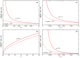
Figure S2: Schematic temperature dependence of the SH conductivity with no disorder effects in the $T$ regime III with $T_{N,C}\rightarrow 0$. (a) The side-jump type contribution $\sigma_{AFM,SH}^{side\,jump}$, (b) the skew-scattering type contribution $\sigma_{AFM,SH}^{skew\,scatt.}$, (c) the side-jump type contribution $\sigma_{FM,SH}^{side\,jump}$, and (d) the skew-scattering type contribution $\sigma_{FM,SH}^{skew\,scatt.}$. The carrier lifetime is modeled as $\tau_{\mathbf{k}}^{-1}=r_{ee}T^{2}+r_{sf}T^{3/2}$ in (a,b), and $\tau_{\mathbf{k}}^{-1}=r_{ee}T^{2}+r_{sf}T^{5/3}$ in (c,d). For the spin-fluctuation contribution, $r_{sf}=0$ is used for solid lines and $\tau_{sf}=0.1$ for dashed lines.

References

- S [1] J. Kondo, Prog. Theor. Phys. 27, 772 (1962).
- S [2] S. Okamoto, T. Egami, and N. Nagaosa, Phys. Rev. Lett. 123, 196603 (2019).
- S [3] T. Moriya, Spin Fluctuations in Itinerant Electron Magnetism, Solid-State Sciences 56 (Springer-Verlag, Berlin, 1985).
- S [4] K. Ueda and T. Moriya, J. Phys. Soc. Jpn. 39, 605 (1975).
- S [5] N. Nagaosa, Quantum Field Theory in Strongly Correlated Electron Systems (Springer-Verlag, Berlin, 1999).
- S [6] P. Wölfle and T. Ziman, Phys. Rev. B 104, 054441 (2021).
- S [7] K. Ueda, J. Phys. Soc. Jpn. 43, 1497 (1997).