Non existence of closed null geodesics in Kerr spacetimes

Abstract.

The Kerr-star spacetime is the extension over the horizons and in the negative radial region of the slowly rotating Kerr black hole. It is known that below the inner horizon, there exist both timelike and null (lightlike) closed curves. Nevertheless, we prove that the null geodesics cannot be closed in the Kerr-star spacetime.

1. Introduction

1.1. Result

Given a spacetime $\big{(}\mathcal{M},\mathbf{g}\big{)}$, i.e. a time-oriented connected Lorentzian manifold, and a geodesic curve $\gamma:I=[a,b]\rightarrow\mathcal{M}$, we say that $\gamma$ is a closed geodesic if $\gamma(a)=\gamma(b)$ and $\gamma^{\prime}(a)=\lambda\gamma^{\prime}(b)\neq 0$, for some real number $\lambda\neq 0$. The purpose of this paper is to prove the non existence of closed null (lightlike) geodesics in the Kerr-star spacetime, which is the extension of the slowly rotating Kerr black hole over the horizons and in the negative radial region. For a detailed construction of the Kerr-star spacetime, see §2.

Theorem 1.1.

Let $K^{*}$ be the Kerr-star spacetime. Then there are no closed null (lightlike) geodesics in $K^{*}$.

1.2. Physical motivation

Kerr spacetimes model the gravitational field in the presence of a rotating black hole (BH), at least sufficiently far away from it. For a precise (attempt of a) definition of BH, see for instance [24]. The recent image of the supermassive black hole at the center of the galaxy M87, which is the first ever direct detection of a BH, obtained by the Event Horizon Telescope Collaboration [18], is in fact consistent with the shadow [5] predicted using the Kerr model. Another empirical motivation comes from the gravitational waves signal detected by the LIGO interferometers [6]: the decay of the waveform agrees with the damped oscillations of a BH relaxing to a final Kerr configuration. The Kerr spacetimes are solutions of Einstein’s vacuum field equations, found by R. P. Kerr [27], which are stationary, axisymmetric and asymptotically flat (see [45]), parametrized by mass parameter $M$ and rotation parameter $a$ (angular momentum per mass unit). They are generalizations of the static spherically symmetric solution of Schwarzschild [39]; indeed, if we set the rotation parameter $a$ to zero, we recover the Schwarzschild spacetime. Notice that the Schwarzschild spacetime is globally hyperbolic (see for instance [29]), hence it is causal, while the slowly rotating Kerr spacetime violates causality as first noticed by Carter [9] (see Ch. $2$ of [35]): both closed timelike and null curves are present. Whether or not causality violating spacetimes can be considered physically reasonable is an open problem. Many classical solutions of the Einstein field equations do violate causality, for instance: van Stockum’s spacetime [44] which have closed timelike curves (CTCs) [43] and closed timelike geodesics (CTGs) [40], Gödel spacetime [20] which presents CTCs but neither closed null geodesics (CNGs) nor CTGs as pointed out by Kundt [28], Chandrasekhar and Wright [11] and then by Nolan in [34], Gott’s spacetime [21] with CTCs. Note that all of these are solutions of non-vacuum Einstein equations: van Stockum’s spacetime in presence of an infinite rotating dust cylinder and zero cosmological constant, Gödel’s solution describes a stationary and homogeneous universe with rotating dust in the presence of non-vanishing cosmological constant, and Gott’s solution contains two moving rotating non-intersecting cosmic strings. Our result shows that the Kerr-star spacetime is a solution of the vacuum Einstein equations containing CTCs but not CNGs, as the solutions found by Li [30] and by Low [31]. Note that the existence of closed null geodesics is also related to the chronology protection conjecture stated by Hawking in [23]. From the physical point of view, closed causal geodesics rise more conceptual problems than closed causal curves, since causal curves correspond to accelerated particles while geodesics are simply free-falling ones. Indeed, for example, it is known for the Gödel spacetime that the required acceleration for such curves is incredibly high (see [34] for a discussion about this). Therefore, the absence of causal geodesics seems to be more physically relevant to ask for, compared to the general causality requirement, in order to get a realistic spacetime model. Notice that we only prove the non existence of closed lightlike geodesics but do not rule out closed timelike geodesics.

1.3. Mathematical motivation: the space of null geodesics

The original motivation which led us to investigate the existence of closed null geodesics in the Kerr spacetime is the study of the space of null (lightlike) geodesics of this spacetime. The ”space of null geodesics” is the space of unparametrized inextendible future pointing null geodesics of a given spacetime. Penrose was the first to suggest the importance of the study of the space of null geodesics [36], [38]. First results in this context were obtained by Low [33]. He proved that if the spacetime is globally hyperbolic (we refer to [2] for causal theory definitions), then its space of null geodesics is contactomorphic to the spherical cotangent bundle of any Cauchy hypersurface of the spacetime, as explained in [32, 12]. For this reason, in the case of globally hyperbolic spacetimes, causality can be described in terms of the geometry of the emerging contact manifold, as shown by Chernov, Nemirovski [14], [13]. In the case of causally simple spacetimes, thanks to the result of Hedicke, Suhr [25], a sufficient condition to get a smooth contact manifold for the space of null geodesics is the existence of a conformal open embedding of the spacetime into a globally hyperbolic one. Furthermore, in [33] it is proven that if $\mathcal{M}$ is a strongly causal spacetime, then its space of null geodesics inherits a smooth structure from the cotangent bundle of $\mathcal{M}$. Nevertheless Low [33] also showed that strong causality is not sufficient to get an Hausdorff topological space. If instead the spacetime is not causal, like Kerr, we have no results which give us informations about its space of null geodesics, except for Zollfrei spacetimes [22, 41], in which all the null geodesics are closed and the space of null geodesics is well understood. From the study of null geodesic orbits we hope to obtain insights into the structure of the space of null geodesics of Kerr spacetimes.

1.4. History of null geodesics in Kerr

Thanks to the existence of three obvious constants of motion (the energy, associated to the timelike Killing vector field, the angular momentum, associated to the spacelike Killing vector field, and the Lorentzian energy of the geodesic), geodesic motion can be solved in some special submanifolds, since in such case three constants of motion are sufficient to completely integrate the system. First Boyer and Price [4], then Boyer and Lindquist [3], and then de Felice [16] studied geodesic motion in the equatorial hyperplane $Eq=\{\theta=\pi/2\}$ in Kerr spacetime [27]. For the same reason, Carter [8] was able to study orbits in the symmetry axis $A=\{\theta=0,\pi\}$. Bounded orbits, namely geodesics which run over a finite interval of radius, were studied by Wilkins [47]. After the maximal analytic extension of the Kerr metric by Boyer and Lindquist [3], Carter [9] found a fourth constant of motion, the Carter constant, which completed the integrability (see for instance [19]) and allowed the study of geodesics in full generality.

The study of the causality of geodesics in the Kerr spacetimes started with the work of Calvani, de Felice, Muchotrzeb, Salmistraro [7]. They considered the fast ($|a|>M$) Kerr spacetime and studied timelike geodesics moving on $\{\theta=\textrm{const}\}$. They found that these geodesics cannot travel back at an earlier time with respect to the starting point. This seemed to suggest that for geodesic motion, there was some kind of obstruction in the violation of causality. For this reason, they conjectured that this would have been a general constraint that saved geodesics from violating causality. However, in a following paper [17], again for the fast Kerr spacetime, Calvani and de Felice showed that this is not true for null geodesics: there exist null geodesics that start their journey at $r=-\infty$, enter the causality violating region, invert their radial motion and go back to asymptotic regions at an earlier time. Note that both [7] and [17] treat the fast Kerr spacetime, i.e. a naked singularity spacetime [37], and not the slow ($|a|<M$) Kerr which is the object of this work and in any case they do not prove the existence of closed causal geodesics.

1.5. Organization of the paper

In §2, we introduce the Kerr metric and discuss the definition and properties of the Kerr-star spacetime. In §3 we recall the set of first order differential equations satisfied by geodesic orbits. In §4, we study the properties of null geodesics required to prove the main theorem. In §5, we give the proof of Thm. 1.1 split into several cases. The overall structure of the proof is detailed in 5.1, 5.3 and Fig. 3.

Acknownledgments

I would like to thank my PhD supervisors S. Nemirovski and S. Suhr for many fruitful discussions and precious advices. I am also grateful to Liang Jin for the interesting and helpful conversations. This research is supported by the SFB/TRR 191 “Symplectic Structures in Geometry, Algebra and Dynamics”, funded by the Deutsche Forschungsgemeinschaft.

2. The Kerr-star spacetime

Consider $\mathbb{R}^{2}\times S^{2}$ with coordinates $(t,r)\in\mathbb{R}^{2}$ and $(\theta,\phi)\in S^{2}$. Fix two real numbers $a\in\mathbb{R}\setminus\{0\}$, $M\in\mathbb{R}_{>0}$ and define the functions

$$\rho(r,\theta):=\sqrt{r^{2}+a^{2}\cos^{2}\theta}$$

and

$$\Delta(r):=r^{2}-2Mr+a^{2}.$$

We study the case $|a|<M$ called slow Kerr, for which $\Delta(r)$ has two positive roots

$$r_{\pm}=M\pm\sqrt{M^{2}-a^{2}}>0$$

and define two sets

• the horizons $\mathscr{H}:=\{\Delta(r)=0\}=\{r=r_{\pm}\}:=\mathscr{H}_{-}\,\sqcup\mathscr{H}_{+}$,

• the ring singularity $\Sigma:=\{\rho(r,\theta)=0\}=\{r=0,\;\theta=\pi/2\}$.

The Kerr metric [27] in Boyer–Lindquist coordinates is

(1) $$\mathbf{g}=-dt\otimes dt+\frac{2Mr}{\rho^{2}(r,\theta)}(dt-a\sin^{2}\theta\;d\phi)^{2}+\frac{\rho^{2}(r,\theta)}{\Delta(r)}dr\otimes dr+a^{2}\sin^{4}(\theta)d\phi\otimes d\phi+\rho^{2}(r,\theta)d\sigma^{2},$$

where $d\sigma^{2}=d\theta\otimes d\theta+\sin^{2}\theta d\phi\otimes d\phi$ is the $2$-dimensional (Riemannian) metric of constant unit curvature on the unit sphere $S^{2}\subset\mathbb{R}^{3}$ written in spherical coordinates.

Remark 2.1.

The components of $\mathbf{g}$ in Boyer–Lindquist coordinates can be read off the common expression

$$\mathbf{g}=- \bigg{(}1-\frac{2Mr}{\rho^{2}(r,\theta)}\bigg{)}\>dt\otimes dt-\frac{4Mar\sin^{2}\theta}{\rho^{2}(r,\theta)}\>dt\otimes d\phi+$$

(2) $$+ \bigg{(}r^{2}+a^{2}+\frac{2Mra^{2}\sin^{2}\theta}{\rho^{2}(r,\theta)}\bigg{)}\sin^{2}\theta\>d\phi\otimes d\phi+\frac{\rho^{2}(r,\theta)}{\Delta(r)}\>dr\otimes dr+\rho^{2}(r,\theta)\>d\theta\otimes d\theta.$$

Nevertheless this last expression does not cover the subsets $\{\theta=0,\pi\}$.

Lemma 2.2.

The metric (1) is a Lorentzian metric on $\mathbb{R}^{2}\times S^{2}\setminus(\Sigma\,\cup\mathscr{H})$.

The sets on which the Boyer–Lindquist coordinates or the metric tensor fail are:

• the horizons $\mathscr{H}=\{\Delta(r)=0\}=\{r=r_{\pm}\}=\mathscr{H}_{-}\sqcup\mathscr{H}_{+}$;

• the ring singularity $\Sigma=\{\rho(r,\theta)=0\}=\{r=0,\;\theta=\pi/2\}$.

In order to extend the metric tensor to the horizons, one has to introduce a new set of coordinates. No change of coordinates can be found in order to extend the metric across the ring singularity. For a detailed study of the nature of the ring singularity, see for instance [15].

Definition 2.3.

The subsets

$$\textrm{I}:=\{r>r_{+}\},\;\textrm{II}:=\{r_{-}<r<r_{+}\},\;\textrm{III}:=\{r<r_{-}\}\subset\{(t,r)\in\mathbb{R}^{2},\;(\theta,\phi)\in S^{2}\}\setminus(\Sigma\,\cup\mathscr{H})$$

are called the Boyer–Lindquist (BL) blocks.

Remark 2.4.

The BL blocks I, II and III are the connected components of $\mathbb{R}^{2}\times S^{2}\setminus(\Sigma\,\cup\mathscr{H})$. Each block with the restriction of the metric tensor (1) is a connected Lorentzian $4$-manifold. To get spacetimes, one has to choose a time orientation on each block.

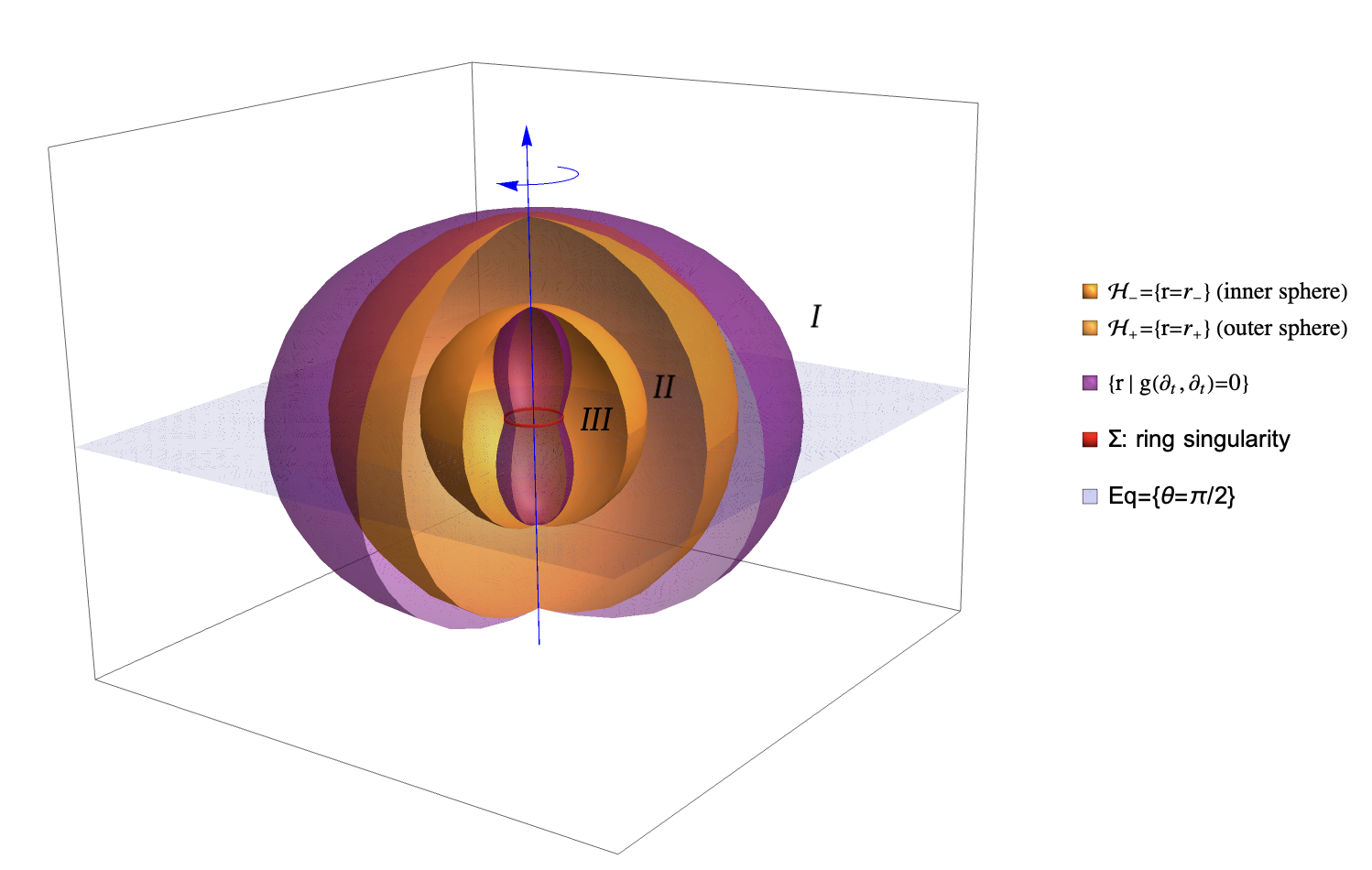
Figure 1. This picture shows a $t$-slice $\{t\}\times\mathbb{R}\times S^{2}$, with the radius drawn as $e^{r}$, so that $r=-\infty$ is at the center of the figure. The Ergoregion $\{\mathbf{g}(\partial_{t},\partial_{t})>0\}$ (at fixed time $t$) is the region between the purple ellipsoids in which $\partial_{t}$ becomes spacelike.

2.1. Time orientation of BL blocks

We define a future time-orientation of block I using the gradient timelike vector field $-\nabla t$. Indeed, the hypersurfaces $\{t=\textrm{const}\}$ are spacelike in block I. Notice that the coordinate vector field $\partial_{t}$ is timelike future-directed for $r\gg r_{+}$ on block I, since $\mathbf{g}(-\nabla t,\partial_{t})=-1$.

We define a time-orientation of block II by declaring the vector field $-\partial_{r}$, which is timelike in II, to be future-oriented.

We define a time-orientation of block III by declaring the vector field $V:=(r^{2}+a^{2})\partial_{t}+a\partial_{\phi}$, which is timelike in III, to be future-oriented.

With this choice of time orientations, each block is a spacetime, i.e. a connected time-oriented Lorentzian $4$-manifold.

2.2. Kerr spacetimes

Definition 2.5.

A Kerr spacetime is an analytic spacetime $(K,g_{K})$ such that

1. there exists a family of open disjoint isometric embeddings $\Phi_{i}\colon\mathcal{B}_{i}\hookrightarrow K$ $(i\in\mathbb{N})$ of BL blocks $(\mathcal{B}_{i},\mathbf{g}_{K}|_{\mathcal{B}_{i}})$, such that $\cup_{i\in\mathbb{N}}\Phi_{i}(\mathcal{B}_{i})$ is dense in $K$;

2. there are analytic functions $r$ and $C$ on K such that their restriction on each $\Phi_{i}(\mathcal{B}_{i})$ of condition $(1)$ is $\Phi_{i}$-related to the Boyer–Lindquist functions $r$ and $C=\cos\theta$ on $\mathcal{B}_{i}$;

3. there is an isometry $\epsilon:K\rightarrow K$ called the equatorial isometry whose restrictions to each BL block sends $\theta$ to $\pi-\theta$, leaving the other coordinates unchanged;

4. there are Killing vector fields $\tilde{\partial_{t}}$ and $\tilde{\partial_{\phi}}$ on K that restrict to the Boyer–Lindquist coordinate vector fields $\partial_{t}$ and $\partial_{\phi}$ on each BL block.

Remark 2.6.

With abuse of notation, we identify each block $\mathcal{B}_{i}$ with its image via the isometric embedding $\Phi_{i}(\mathcal{B}_{i})\subset K$.

Lemma 2.7.

Each time-oriented BL block is a Kerr spacetime.

Definition 2.8.

In a Kerr spacetime K, on any BL block $\mathcal{B}_{i}$

1. the axis $A=\{\theta=0,\pi\}$ is the set of zeroes of the Killing vector field $\tilde{\partial_{\phi}}$ as in $(4)$ of Def. 2.5;

2. the equatorial hyperplane $Eq=\{\theta=\pi/2\}$ is the set of fixed points of the equatorial isometry $\epsilon$ as in $(3)$ of Def. 2.5.

2.3. The Kerr-star spacetime

Definition 2.9.

On each BL block, we define the Kerr-star coordinate functions:

(3) $$t^{*}:=t+\mathcal{T}(r)\in\mathbb{R},\hskip 28.45274pt\phi^{*}:=\phi+\mathcal{A}(r)\in S^{1},$$

with $d\mathcal{T}/dr:=(r^{2}+a^{2})/\Delta(r)$ and $d\mathcal{A}/dr:=a/\Delta(r)$.

Lemma 2.10 ([35], Lemma $2.5.1$).

For each BL block $B$, the map $\xi^{*}=(t^{*},r,\theta,\phi^{*}):B\setminus A\rightarrow\xi^{*}(B)\subseteq\mathbb{R}^{4}$ is a coordinate system on $B\setminus A$, where $A$ is the axis. We call $\xi^{*}$ a Kerr-star coordinate system.

Because the Kerr-star coordinate functions differ from BL coordinates only by additive functions of $r$, the coordinate vector fields $\partial_{t},\partial_{\theta},\partial_{\phi}$ are the same in the two systems, except that in $K^{*}$ they extend over the horizons. Instead, the new coordinate vector field $\partial^{*}_{r}=\partial_{r}-\Delta(r)^{-1}V$, where $V$ is one of the canonical vector fields defined in Section 3. Note that if we use Kerr-star coordinates, we get $\mathbf{g}(\partial^{*}_{r},\partial^{*}_{r})=0$, i.e. $\partial^{*}_{r}$ is a null vector field of $K^{*}$, while in BL coordinates, $\mathbf{g}(\partial_{r},\partial_{r})=\rho^{2}(r,\theta)/\Delta(r),$ which is singular when $\Delta(r)=0$.

Lemma 2.11.

The Kerr metric, expressed in Kerr-star coordinates, takes the form

$$\mathbf{g}= -\bigg{(}1-\frac{2Mr}{\rho^{2}(r,\theta)}\bigg{)}\>dt^{*}\otimes dt^{*}-\frac{4Mar\sin^{2}\theta}{\rho^{2}(r,\theta)}\>dt^{*}\otimes d\phi^{*}\,+$$

(4) $$+\bigg{(}r^{2}+a^{2}+\frac{2Mra^{2}\sin^{2}\theta}{\rho^{2}(r,\theta)}\bigg{)}\sin^{2}\theta\>d\phi^{*}\otimes d\phi^{*}+2\>dt^{*}\otimes dr\,+$$

$$-2a\sin^{2}\theta\>d\phi^{*}\otimes dr+\rho^{2}(r,\theta)\>d\theta\otimes d\theta.$$

Now all coefficients in $\mathbf{g}$ are well defined on the horizons $\mathscr{H}=\{\Delta(r)=0\}$, hence it is a well defined Lorentzian metric on $\mathbb{R}^{2}\times S^{2}\setminus\Sigma$ and constitutes an analytic extension of (1) over $\mathscr{H}$.

Definition 2.12.

The Kerr-star spacetime is a Kerr spacetime as defined in 2.5 given by the tuple $(K^{*},\mathbf{g},o)$ with $K^{*}=\{(t^{*},r)\in\mathbb{R}^{2},\,(\theta,\phi^{*})\in S^{2}\}\setminus\Sigma$, $\mathbf{g}$ as in Lemma 2.11 (extended over the axis) and $o$ is the future time-orientation induced by the null vector field $-\partial^{*}_{r}.$

Remark 2.13.

Note that the time-orientations on individual BL blocks agree with the ones defined for the Kerr-star spacetime: $\mathbf{g}(-\partial^{*}_{r},\partial_{t})=-1<0$ on I, $\mathbf{g}(-\partial^{*}_{r},-\partial_{r})=\mathbf{g}(\partial_{r},\partial_{r})=\rho^{2}(r,\theta)/\Delta(r)<0$ on II and $\mathbf{g}(-\partial^{*}_{r},V)=\frac{1}{\Delta(r)}\mathbf{g}(V,V)=-\rho^{2}(r,\theta)<0$ on III.

2.4. Totally geodesic submanifolds of the Kerr-star spacetime

Lemma 2.14.

Let $K^{*}$ be the Kerr-star spacetime as in Def. 2.12. The axis $A$ and the equatorial hyperplane $Eq$ of $K^{*}$ are closed totally geodesic submanifolds of $K^{*}$.

Proposition 2.15.

[35] Let $K^{*}$ be the Kerr-star spacetime. Then the horizon $\mathscr{H}$ is a closed totally geodesic null hypersurface, with future hemicone on the $-\partial^{*}_{r}$ side. Moreover, the restriction of $V:=(r^{2}+a^{2})\partial_{t}+a\partial_{\phi}$ (called canonical vector field in §3) on $\mathscr{H}$ is the unique null vector field on $\mathscr{H}$ that is tangent to $\mathscr{H}$, hence also normal to $\mathscr{H}$.

2.5. Causal region of the Kerr-star spacetime

Proposition 2.16 ([35], Proposition $2.4.6$).

The BL blocks I and II are causal.

Corollary 2.17.

Let $K^{*}$ be the Kerr-star spacetime. Then the region
I$\;\cup$ II$\;\cup\;\{r=r_{\pm}\}=\{t^{*}\in\mathbb{R},r\in[r_{-},+\infty),(\theta,\phi^{*})\in S^{2}\}\setminus\Sigma\subset K^{*}$ is causal.

Proof.

Let $\gamma$ be a future pointing curve. If $\gamma$ is entirely contained either in I or in II, then by Prop. 2.16, $\gamma$ cannot be closed. If $\gamma$ is entirely contained in $\mathscr{H}=\{r=r_{\pm}\}$ (closed totally geodesic null hypersurface of $K^{*}$ by Prop. 2.15), then by Lem. $1.5.11$ of [35], except for restphotons, all other curves are spacelike, but restphotons are integral curves of $V|_{\mathscr{H}}=(r^{2}_{\pm}+a^{2})\partial_{t}+a\partial_{\phi}$, which cannot be closed. Since the time orientation $-\partial^{*}_{r}$ is null and transverse to the null hypersurface $\mathscr{H}$, the future directed curves always go in the direction of $-\partial^{*}_{r}$, if they hit $\mathscr{H}$ transversally. Henceforth, if $\gamma$ starts in the BL block I (II), crosses $\mathscr{H}_{+}$ ($\mathscr{H}_{-}$) transversally, enters the block II (III), then $\gamma$ cannot re-intersect $\mathscr{H}_{+}$ from II to I ($\mathscr{H}_{-}$ from III to II). The last possibility is the following: $\gamma$ starts in I (II), becomes tangent to $\mathscr{H}_{+}$ ($\mathscr{H}_{-}$), hence either lies forever on $\mathscr{H}_{+}$ ($\mathscr{H}_{-}$) or leaves it at some point. In the first case, $\gamma$ is obviously not closed, while in the second, it cannot be closed because it will necessarily have to enter the region $\{r<r_{+}\}$ ($\{r<r_{-}\}$), according to the time orientation. ∎

3. Geodesics in Kerr spacetimes

3.1. Constants of motion

Let $(K,\mathbf{g})$ be a Kerr spacetime as in Def. 2.5. Recall that there are two Killing vector fields $\tilde{\partial_{t}}$ and $\tilde{\partial_{\phi}}$ on $K$.

Definition 3.1 (Energy and angular momentum).

For a geodesic $\gamma$ of $(K,\mathbf{g})$, the constants of motion

$$E=E(\gamma):=-\mathbf{g}(\gamma^{\prime},\tilde{\partial_{t}})$$

and

$$L=L(\gamma):=\mathbf{g}(\gamma^{\prime},\tilde{\partial_{\phi}})$$

are called its energy and its angular momentum (around the axis of rotation of the black hole), respectively.

Definition 3.2.

For every BL block $\mathcal{B}_{i}$ define the canonical vector fields

$$V:=(r^{2}+a^{2})\partial_{t}+a\partial_{\phi}\quad\text{ and }\quad W:=\partial_{\phi}+a\sin^{2}\theta\,\partial_{t}$$

via the isometry $\Phi_{i}\colon\mathcal{B}_{i}\hookrightarrow K$.

Remark 3.3.

$V$ and $W$ are not Killing vectors.

Definition 3.4.

Let $\gamma$ be a geodesic in $K$ with energy $E$ and angular momentum $L$. Define the functions $\mathbb{P}$ and $\mathbb{D}$ along $\gamma$ by

$$\mathbb{P}(r):=-\mathbf{g}(\gamma^{\prime},V)=(r^{2}+a^{2})E-La$$

and

$$\mathbb{D}(\theta):=\mathbf{g}(\gamma^{\prime},W)=L-Ea\sin^{2}\theta.$$

A geodesic in a Kerr spacetime has two additional constants of motions. First, there is the Lorentian energy $q:=\mathbf{g}(\gamma^{\prime},\gamma^{\prime})$, which is always constant along every geodesic in any pseudo-Riemannian manifold. The second one is $K$, which was first found by Carter in [9] using the separability of the Hamilton–Jacobi equation. $K$ can be defined (see Ch. $7$ in [10]) by

$$K:=2\rho^{2}(r,\theta)\mathbf{g}(l,\gamma^{\prime})\mathbf{g}(n,\gamma^{\prime})+r^{2}q,$$

where $l=\frac{1}{\Delta(r)}V+\partial_{r}$ and $n=\frac{1}{2\rho^{2}(r,\theta)}V-\frac{\Delta(r)}{2\rho^{2}(r,\theta)}\partial_{r}$. See also [46] for a definition using a Killing tensor for the Kerr metric.

Definition 3.5 (Carter constant).

On a Kerr spacetime, the constant of motion

$$Q:=K-(L-aE)^{2}\hskip 14.22636pt\textrm{or}\hskip 14.22636pt\mathcal{Q}:=Q/E^{2}\hskip 8.5359pt\textrm{if}\hskip 8.5359ptE\neq 0$$

is called the Carter constant.

3.2. Equations of motion

Proposition 3.6 ([35], Proposition $4.1.5$, Theorem $4.2.2$).

Let $B$ be a BL block and $\gamma$ be a geodesic with initial position in $B\subset K$ and constants of motion $E,L,Q,q$. Then the components of $\gamma$ in the BL coordinates $(t,r,\theta,\phi)$ satisfy the following set of first order differential equations

(5) $$\begin{cases}\rho^{2}(r,\theta)\phi^{\prime}=\frac{\mathbb{D}(\theta)}{\sin^{2}\theta}+a\frac{\mathbb{P}(r)}{\Delta(r)}\\ \rho^{2}(r,\theta)t^{\prime}=a\mathbb{D}(\theta)+(r^{2}+a^{2})\frac{\mathbb{P}(r)}{\Delta(r)}\\ \rho^{4}(r,\theta)r^{\prime 2}=R(r)\\ \rho^{4}(r,\theta)\theta^{\prime 2}=\Theta(\theta)\end{cases}$$

where

$$R(r):= \Delta(r)\left[(qr^{2}-K(E,L,Q)\right]+\mathbb{P}^{2}(r)=$$

$$= (E^{2}+q)r^{4}-2Mqr^{3}+\mathfrak{X}(E,L,Q)r^{2}+2MK(E,L,Q)r-a^{2}Q,$$

$$\Theta(\theta):= K(E,L,Q)+qa^{2}\cos^{2}\theta-\frac{\mathbb{D}(\theta)^{2}}{\sin^{2}\theta}=$$

$$= Q+\cos^{2}\theta\left[a^{2}(E^{2}+q)-L^{2}/\sin^{2}\theta\right],$$

with

$$\mathfrak{X}(E,L,Q):=a^{2}(E^{2}+q)-L^{2}-Q\text{, and }K(E,L,Q)=Q+(L-aE)^{2}.$$

Remark 3.7.

Since in the third and in the fourth differential equations of Prop. 3.6 the left-hand sides are clearly non-negative, we see that the polynomials $R(r)$ and $\Theta(\theta)$ are non-negative along the geodesics. Hence the geodesic motion can only happen in the $r,\theta$-region for which $R(r),\Theta(\theta)\geq 0$.

In order to study geodesics that cross the horizons

$$\mathscr{H}=\{\Delta(r)=0\}=\{r=r_{\pm}\},$$

it is necessary to introduce the Kerr-star coordinate system. Note however that since the change of coordinates modifies only the $t$ and the $\phi$ coordinates and the $r,\theta$-differential equations do not involve $t$ and $\phi$, the last two differential equations do extend over $\mathscr{H}$. Observe also that the $r,\theta$- differential equations are not singular on $\mathscr{H}$, while the $t,\phi$-differential equations are.

Notice that $\Theta(\theta)$ is also well-defined if the null geodesic crosses $A=\{\theta=0,\pi\}$. Indeed, $L=0$ (because $\tilde{\partial_{\phi}}\equiv 0$ on $A$), hence $\mathbb{D}(\theta)=-Ea\sin^{2}\theta$, and then

$$\Theta(\theta)=K(E,0,Q)-(-Ea\sin^{2}\theta)^{2}/\sin^{2}\theta=Q+a^{2}E^{2}-a^{2}E^{2}\sin^{2}\theta=Q+a^{2}E^{2}\cos^{2}\theta.\\$$

Thus the $r,\theta$-differential equations can be used to study geodesics on the whole Kerr-star spacetime.

Remark 3.8.

The system (5) is composed of first order differential equations, while the geodesic equation is second order. There exist solutions of (5), called singular, which do not correspond to geodesics. For example, if $r_{0}\in\mathbb{R}$ is a multiplicity one zero of $r\mapsto R(r)$, then $r_{0}$ solves the radial equation in (5), since in this case $r^{\prime}(s)=0$ for all $s$, but we do not have a geodesic.

3.3. Dynamics of geodesics

The non-negativity of $R(r)$ and $\Theta(\theta)$ in the first order differential equations of motion (5) can be used to study the dynamics of the $r,\theta$-coordinates of the geodesics, together with the next proposition.

Proposition 3.9 ([35], Corollary $4.3.8$).

Suppose $R(r_{0})=0$. Let $\gamma$ be a geodesic whose $r$-coordinate satisfies the initial conditions $r(s_{0})=r_{0}$ and $r^{\prime}(s_{0})=0$.

1. If $r_{0}$ is a multiplicity one zero of $R(r)$, i.e. $R^{\prime}(r_{0})\neq 0$, then $r_{0}$ is an $r$-turning point, namely $r^{\prime}(s)$ changes sign at $s_{0}$.

2. If $r_{0}$ is a higher order zero of $R(r)$, i.e. at least $R^{\prime}(r_{0})=0$, then $\gamma$ has constant $r(s)=r_{0}$.

Analogous results hold for $r$ and $R(r)$ replaced by $\theta$ and $\Theta(\theta)$.

4. Properties of null geodesics in Kerr spacetimes

4.1. Principal geodesics

Since the vector fields $V,W,\partial_{r},\partial_{\theta}$ are mutually orthogonal, the tangent vector to a geodesic $\gamma$ can be decomposed as $\gamma^{\prime}=\gamma^{\prime}_{\Pi}+\gamma^{\prime}_{\perp}$ where $\Pi:=span\{\partial_{r},V\}$ (timelike plane) and $\Pi^{\perp}:=span\{\partial_{\theta},W\}$ (spacelike plane).

Definition 4.1.

A Kerr geodesic $\gamma$ is said to be principal if $\gamma^{\prime}=\gamma^{\prime}_{\Pi}$.

Proposition 4.2 ([35], Corollary $4.2.8(2)$).

If $\gamma$ is a null geodesic, then $K\geq 0$, and
$K=0\Longleftrightarrow\;$ $\gamma$ is principal.

Definition 4.3.

A null geodesic is called a restphoton if it lies in $\mathcal{H}$.

Restphotons are integral curves of $V|_{\mathcal{H}}$ by Prop. 2.15.

Proposition 4.4 ([35], Lemma $4.2.9(3,4)$).

For a null geodesic $\gamma$,

1. $K=L=0$ but $E\neq 0\Leftrightarrow\gamma\in A\setminus\mathcal{H}$.

2. $K=L=E=0\Leftrightarrow$ $\gamma$ is a restphoton.

4.2. Null geodesics with $Q<0$

Proposition 4.5.

Let $\gamma$ be a null geodesic with $Q<0$. Then

1. $\gamma$ does not intersect $Eq=\{\theta=\pi/2\}$;

2. $a^{2}E^{2}>L^{2}$ and in particular $E\neq 0$.

Proof.

If $\gamma\cap A=\emptyset$, then from the $\theta$-equation of (5) we have

$$\cos^{2}\theta[L^{2}/\sin^{2}\theta-a^{2}E^{2}]=Q-\rho^{4}(r,\theta)\theta^{\prime 2}<0.$$

Hence $\cos^{2}\theta\neq 0$ and $L^{2}/\sin^{2}\theta-a^{2}E^{2}<0$, hence $\gamma\cap Eq=\emptyset$ and $a^{2}E^{2}>L^{2}$, so $E\neq 0$.

If $\gamma\cap A\neq\emptyset$, then by Prop. 4.4 $L=0$ and

$$-a^{2}E^{2}\cos^{2}\theta=Q-\rho^{4}(r,\theta)\theta^{\prime 2}<0.$$

Therefore $\cos^{2}\theta\neq 0$ and $a^{2}E^{2}>0$, so $\gamma\cap Eq=\emptyset$ and $E\neq 0$. ∎

Remark 4.6.

If a geodesic $\gamma$ has $Q>0$, then its $\theta$-motion is an oscillation around $\theta=\pi/2$, so it cuts repeatedly through $Eq$ (see Propositions $4.5.4,4.5.5$ in [35]).

Proposition 4.7.

For $Q<0$ null geodesics, $R(r)$ has either zero or two negative roots.

Proof.

First we show that $R(r)$ does not have zeroes in $r\geq 0$. It is sufficient to show that every coefficient of the polynomial function $R(r)$ is non-negative, with at least one positive. We know from Prop. 3.6 that for null geodesics

(6) $$R(r)=E^{2}r^{4}+\mathfrak{X}r^{2}+2MKr-a^{2}Q.$$

From Prop. 4.5 and Prop. 4.2, we see that the coefficients are

• $E^{2}>0$ at $r^{4}$;

• $\mathfrak{X}=a^{2}E^{2}-L^{2}-Q>-Q>0$ at $r^{2}$;

• $K\geq 0$ at $r$;

• $-a^{2}Q>0$ at $r^{0}$.

We now show that $R(r)$ has at most two real zeroes. We have $R^{\prime}=4E^{2}r^{3}+2\mathfrak{X}r+2MK$, hence $R^{\prime\prime}=12E^{2}r^{2}+2\mathfrak{X}$. Since $\mathfrak{X}>0$, $R^{\prime\prime}$ never vanishes and $R^{\prime\prime}(0)=2\mathfrak{X}>0$. Then $R^{\prime\prime}>0$ everywhere, which means that $R^{\prime}$ has a unique zero. This implies that $R(r)$ has a unique critical point and hence we have either $0$ or $2$ roots, which have to be negative.

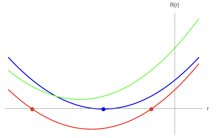
Figure 2. For $Q<0$ null geodesics, $R(r)$ has either zero or two negative roots (multiplicity two is allowed).

∎

5. Proof of Theorem 1.1

5.1. Strategy of the proof

Let $\gamma\colon I\to K^{*}$ be a closed null geodesic (CNG). Since the radius function $r\colon K^{*}\to\mathbb{R}$ is everywhere smooth the composition $r\circ\gamma$ has at least two critical points $s_{0}<s_{1}$ in each period $[a,a+T)$, i.e. $(r\circ\gamma)^{\prime}(s_{0})=(r\circ\gamma)^{\prime}(s_{1})=0$. Since $\rho\colon K^{*}\to\mathbb{R}$ does not vanish on $K^{*}$ the differential equation for $r\circ\gamma$

$$(\rho\circ\gamma)^{4}[(r\circ\gamma)^{\prime}]^{2}=R(r\circ\gamma)$$

implies that $R(r\circ\gamma(s_{0,1}))=0$. Because of the differential equation, the geodesic motion must happen in the $r$-region on which $R(r\circ\gamma)\geq 0$. Further since $R$ is a polynomial in $r$ we can distinguish two cases:

1. The zeros $r\circ\gamma(s_{0,1})$ of $R$ are simple, i.e. $dR/dr\neq 0$ at these points. Then $r\circ\gamma(s_{0,1})$ are turning points of $r\circ\gamma$, i.e. $(r\circ\gamma)^{\prime}$ changes its sign at $s_{0}$ and $s_{1}$.

2. One of the zeros $r\circ\gamma(s_{0})$ or $r\circ\gamma(s_{1})$ is a higher order zero of $R$. Then $r\circ\gamma$ is constant.

Both the two facts follow from Proposition 3.9.

Most possible CNGs can be ruled out by comparing the location of the zeros of $R(r)$ with the following consequence of the causal structure of Kerr:

Lemma 5.1.

Let $\gamma\colon I\to K^{*}$ be a closed null geodesic. Then $r\circ\gamma\subset\{r<r_{-}\}$.

Proof.

The region

$$\{r\geq r_{-}\}=\{t^{*}\in\mathbb{R},r\in[r_{-},+\infty),(\theta,\phi^{*})\in S^{2}\}\setminus\Sigma\subset K^{*}$$

is causal by Corollary 2.17 and closed null geodesics cannot intersect $\{r=r_{-}\}$ by Prop. 5.2. ∎

There are two cases in which we need additional arguments:

1. to exclude CNGs with $Q>0$ confined in $\{0<r<r_{-}\}$, we use the fact that this region of the spacetime is foliated by spacelike hypersurfaces.

2. To exclude CNGs with $Q<0$ and $r=\textrm{const}<0$, we show that the $\theta$-coordinate of such a geodesic is periodic whereas the $t$-coordinate is quasi-periodic with a non-zero increment, see 5.5.3.

5.2. Horizons and Axis cases

First we rule out CNGs entirely contained in the axis $A=\{\theta=0,\pi\}$ and CNGs entirely contained/intersecting the horizon $\mathscr{H}=\{r=r_{\pm}\}$.

The case of the horizon $\mathscr{H}=\{r=r_{\pm}\}$

Proposition 5.2.

There are no CNGs intersecting $\mathscr{H}=\{r=r_{\pm}\}$.

Proof.

On the submanifolds $W:=\{r=\textrm{const}\}$, we have $\textrm{det}\;g^{*}|_{W}=-\rho^{2}(r,\theta)\Delta(r)\sin^{2}\theta$, where $g^{*}$ is the Kerr-star coordinates expression of $\mathbf{g}$. Therefore the metric $g^{*}$ degenerates on the tangent spaces to $\mathscr{H}=\{\Delta(r)=0\}=\{r=r_{\pm}\}$. Therefore $T_{p}\mathscr{H}$ is a null subspace of $T_{p}K^{*}$ for every $p\in K^{*}$, i.e. the submanifolds $\mathscr{H}=\{\Delta(r)=0\}$ are null hypersurfaces. Then, by Lem. $1.5.11$ of [35], every vector in $T_{p}K^{*}$ is spacelike, except for the intersection of $T_{p}\mathscr{H}$ with the null cone of $T_{p}K^{*}$. Note that the vector field $V=(r^{2}+a^{2})\partial_{t}+a\partial_{\phi}$ is tangent to $\mathscr{H}$ and we have $\mathbf{g}(V,V)=-\Delta(r)\rho^{2}(r,\theta)$, i.e. $V$ is null along $\mathscr{H}$. Hence $V|_{\mathscr{H}}$ generates the unique null tangent line to $H$. Further note that no flowline of $V$ closes. By Prop. 2.15, the flowlines of $V|_{\mathscr{H}}$ are null pregeodesics, hence the null geodesics tangent to $\mathscr{H}$ do not close.

It remains to consider null geodesics intersecting $\mathscr{H}$ transversally. Since each connected component $\{r=r_{\pm}\}$ of $\mathscr{H}$ is an orientable hypersurface separating the orientable manifold $K^{*}$, every closed curve transversal to $H$ has to intersect $\{r=r_{\pm}\}$ an even number of times. Further since $K^{*}$ is time-oriented by $-\partial_{r}^{*}$, all tangent vectors to a null geodesics transversal to $H$ have to lie on one side of $H$. Therefore a null geodesic transversal to $H$ can intersect each connected component $\{r=r_{\pm}\}$ only once. This shows that no null geodesic transversal to $\mathscr{H}$ can close. ∎

The case of the axis $A=\{\theta=0,\pi\}$

Proposition 5.3.

There are no CNGs which are tangent at some point to $A=\{\theta=0,\pi\}$. In particular, there are no CNGs entirely contained in $A$.

Proof.

First of all, $A=\{\theta=0,\pi\}$ is a $2$-dimensional closed totally geodesic submanifold by Lem. 2.14. Hence if a geodesic $\gamma$ is tangent to $A$ at some point, it will always lie on $A$. By Prop. 4.4, if $\gamma\in A$, then $L=K=0$. Hence there are two possible cases: if $E=0$, by Prop. 4.4, then $\gamma$ is a restphoton, i.e. an integral curve of $V|_{\mathscr{H}}=(r_{\pm}^{2}+a^{2})\partial_{t}+a\partial_{\phi}$, which is not closed. If $E\neq 0$, then using (5), we have

$$R(r)=E^{2}(r^{2}+a^{2})^{2}>0.$$

So $R(r)$ has no zeroes and therefore the geodesics cannot be bounded.

∎

5.3. Steps of the proof for other cases

The proof splits into two main cases $E=0$ and $E\neq 0$.

If $E=0$ (5.4), we analyse two subcases $L^{2}+Q=0$ and $L^{2}+Q\neq 0$ (this last splits into $L\neq 0$ and $L=0$).

If $E\neq 0$ (5.5), we analyse three subcases $Q=0$ (5.5.1), $Q>0$ (5.5.2) with $Q<0$ (5.5.3).

Remark 5.4.

The only case which requires a detailed analysis of the differential equations is the case $E\neq 0$ and $Q<0$ (see 5.5.3).

Figure 3. All the geodesic types which have to be studied.

5.4. Case $E=0$

From Prop. 3.6, for null $(q=0)$ geodesics we have

(7) $$R(r) =\mathfrak{X}(0,L,Q)r^{2}+2MK(0,L,Q)r-a^{2}Q\geq 0,$$

(8) $$\Theta(\theta) =Q-\frac{\cos^{2}\theta}{\sin^{2}\theta}L^{2}\geq 0,$$

with $\mathfrak{X}(0,L,Q)=-(L^{2}+Q)$ and $K(0,L,Q)=L^{2}+Q$, i.e. $\mathfrak{X}=-K$. Notice that we must have $Q\geq 0$ by (8), hence $L^{2}+Q\geq 0$.

5.4.1. Subcase $L^{2}+Q=0$

We have

(9) $$R(r)=-a^{2}Q\geq 0.$$

Since $Q\geq 0$, the only possibility is $Q=0$, hence $L=0$ by (8). Moreover we must have $\rho(r,\theta)^{4}r^{\prime 2}=R(r)\equiv 0$, hence $r(s)=\textrm{const}$. However, by Prop. 4.4, we know that a null geodesic with $L=E=K=0$ is a restphoton, i.e. an integral curve of the canonical vector field $V|_{\mathscr{H}}=(r^{2}_{\pm}+a^{2})\partial_{t}+a\partial_{\phi}$. Since $r(s)=r_{\pm}=\textrm{const}$, this integral curve would be $\bigg{(}(r^{2}_{\pm}+a^{2})s+c_{t},\;r_{\pm},\;\theta_{0},\;as+c_{\phi}\bigg{)}$ with $c_{t}\in\mathbb{R},\theta_{0}\in[0,\pi],c_{\phi}\in S^{1}$, which is clearly not closed.

5.4.2. Subcase $L^{2}+Q\neq 0$

Then we must have $L^{2}+Q>0$. Since $|a|<M$ and $L^{2}+Q>Q\geq 0$, the discriminant of (7) is $\textrm{dis}=4M^{2}(L^{2}+Q)^{2}-4a^{2}Q(L^{2}+Q)>0$. Therefore $R(r)$ has two roots given by

$$M\pm\sqrt{M^{2}-\frac{a^{2}Q}{L^{2}+Q}}.$$

If $L\neq 0$,

then we have (see Figures 4, 5)

$$M+\sqrt{M^{2}-\frac{a^{2}Q}{L^{2}+Q}}>r_{+}=M+\sqrt{M^{2}-a^{2}}.$$

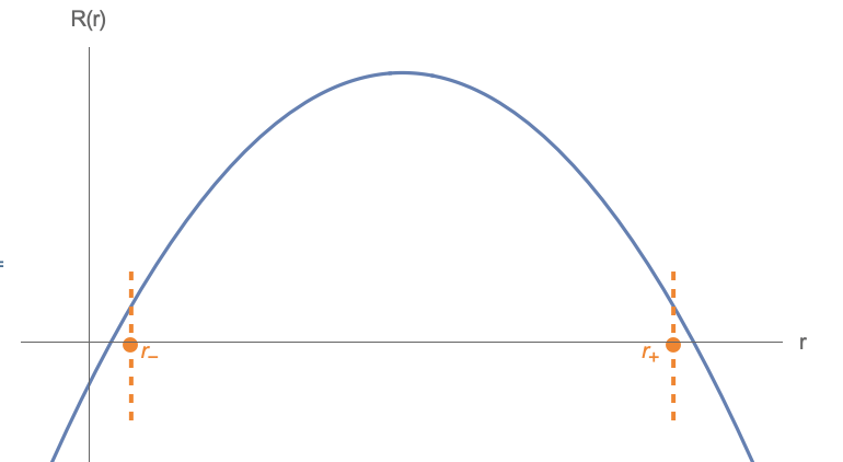
Figure 4. Plot of $R(r)$ in the case $E=0,\;L^{2}+Q\neq 0,\;Q>0$
with $a=3,M=6,L=2,Q=4$.

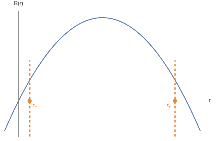
Figure 5. Plot of $R(r)$ in the case $E=0,\;L^{2}+Q\neq 0,\;Q=0$
with $a=3,M=6,L=2,Q=0$.

So if $L\neq 0$, the geodesics will have to cross $\mathscr{H}$ since one of the two zeros is bigger than $r_{+}$ and the other is smaller than $r_{-}$, which is impossible for a CNG by Prop. 5.2.

If $L=0$,

then $Q>0$, hence $R^{\prime\prime}(r)=-2Q<0$. Moreover $R(r)=-Q\Delta(r)$ because $E=L=0$. Therefore the two (multiplicity one) roots are $r_{-}$ and $r_{+}$ (see Fig. 6).

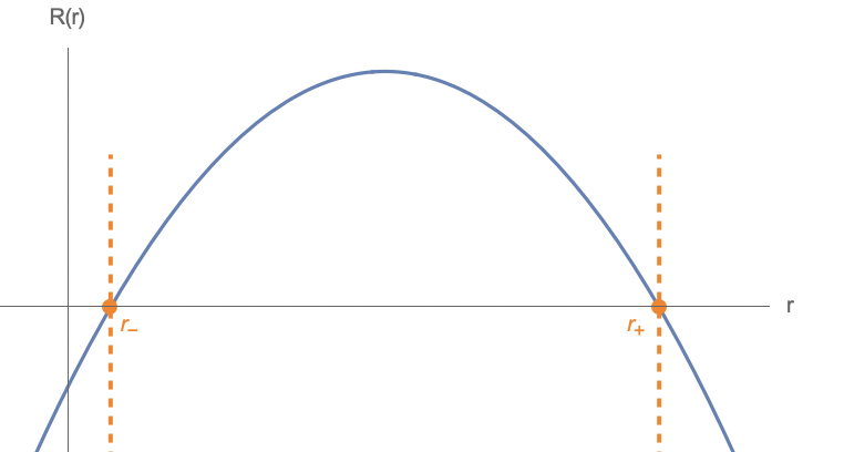
Figure 6. Plot of $R(r)$ in the case $E=0,\;L^{2}+Q\neq 0,\;L=0$
with $a=3,M=6,L=0,Q=4$.

This polynomial $R(r)$ cannot produce a CNG since the hypersurfaces $\mathscr{H}=\{r=r_{\pm}\}$ are closed totally geodesic submaninfolds by Prop. 2.15 and a geodesic cannot have turning points on such hypersurfaces because it would be tangent to them there.

5.5. Case $E\neq 0$

5.5.1. Subcase $Q=0$

We have

(10) $$R(r) =E^{2}r^{4}+(a^{2}E^{2}-L^{2})r^{2}+2M(L-aE)^{2}r\geq 0.$$

From the $\theta$-equation, since $Q=0$, we get

$$a^{2}E^{2}\geq\frac{L^{2}}{\sin^{2}\theta}\geq L^{2}.$$

Observe that

$$R(0) =0,$$

$$R^{\prime}(r) =4E^{2}r^{3}+2(a^{2}E^{2}-L^{2})r+2M(L-aE)^{2},$$

$$R^{\prime\prime}(r) =12E^{2}r^{2}+2(a^{2}E^{2}-L^{2})\geq 0.$$

Therefore $R$ is convex and can only produce bounded radial behaviour with constant $r(s)\equiv 0$ if $r=0$ is a multiple root of $R(r)$, i.e. if $L=aE$. The polynomial reduces then to $R(r)=E^{2}r^{4}$. But $\Theta(\theta)=-\frac{\cos^{4}\theta}{\sin^{2}\theta}L^{2}\geq 0$ and $L\neq 0$, hence we can only have $\theta(s)=\pi/2\equiv\textrm{const}$, which is not possible because the geodesic would then intersect the ring singularity (see Fig.7).

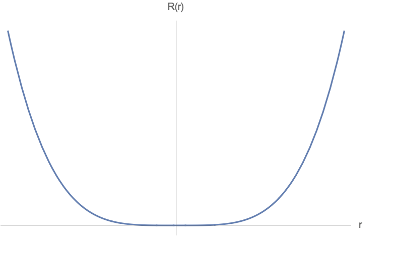
Figure 7. Plot of $R(r)$ in the case $E\neq 0,\;Q=0,\;L=aE\neq 0$ with $a=3,$
$M=10,E=5,Q=0,L=15$.

5.5.2. Subcase $Q>0$

From Prop. 4.2, we know that for null geodesics $K=Q+(L-aE)^{2}\geq 0$. Hence if $Q>0$, then $K>0.$ Let us again consider $R(r)=E^{2}r^{4}+\mathfrak{X}(E,L,Q)r^{2}+2MK(E,L,Q)r-a^{2}Q$. Since $R(0)=-a^{2}Q<0$, if a null geodesic has bounded radial behaviour either it must be confined entirely in the negative region or entirely in the positive region, since we must have $R(r)\geq 0$. Bounded radial behaviour in the negative region is impossible in this subcase. Indeed, the signs of the coefficients of $R(-r)$ are $+\;\textrm{sign}(\mathfrak{X})\;-\;-$, so for every sign of $\mathfrak{X}$, there would be only one change of sign, hence there can be only one single real negative root by the ”Descartes’ rule of signs”.

Remark 5.5.

The same conclusion about the sign of the coefficients of $R(r)$ also holds in the case $L=aE$, indeed $R(r)=E^{2}r^{4}-Qr^{2}+2MQr-a^{2}Q$ in such a case.

By Lem. 5.1, we could only have a bounded (either in a compact $r$-interval or constant $r$) radial behaviour in the positive region $\{0<r<r_{-}\}$. However the hypersurfaces $\mathcal{N}:\{t=t_{0}\}\cap\{0<r<r_{-}\}$ are spacelike. Indeed, if $p\in\mathcal{N}\setminus A$, where $A=\{\theta=0,\pi\}$, then $T_{p}\mathcal{N}$ is spanned by $\partial_{r},\partial_{\theta},\partial_{\phi}$ which are spacelike and orthogonal to each other. If $p\in A\subset\mathcal{N}$, then $p=(t_{0},r,q)$ with $q=(0,0,\pm 1)\in S^{2}$, and we may replace $\partial_{\theta},\partial_{\phi}$ by any basis of $T_{q}S^{2}$. Hence we cannot have CNGs in $\{0<r<r_{-}\}$ because otherwise there would be a point on a spacelike hypersurface $\{t=t_{0}\}$ at which the null tangent vector of the geodesic would be tangent to this hypersurface.

5.5.3. Subcase $Q<0$

This is the last remaining case and the most difficult one. By Prop. 4.7, the only possible bounded behaviour is $r(s)=\textrm{const}<0$ (see Fig.8). Such geodesics are known in the literature as spherical geodesics, see e.g. [42].

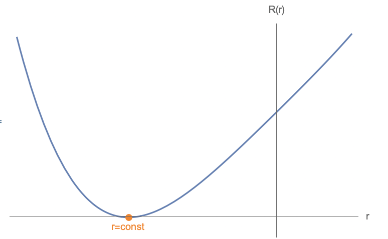
Figure 8. Plot of $R(r)$ in the case $E\neq 0$, $Q<0$ with $a=\frac{1}{\sqrt{2}},M=\frac{6}{\sqrt{23}},E=1,$
$L=3\sqrt{\frac{23}{2}},Q=-104$.

By Prop. 4.5, null geodesics with negative Carter constant do not meet $Eq=\{\theta=\pi/2\}$, hence $\cos^{2}\theta\neq 0$. Then we may define $u:=\cos^{2}\theta\in(0,1]$. Since we are in the case $E\neq 0$, we can re-write the $\theta$-equation in (5) as

(11) $$\bigg{(}\frac{\rho^{2}(r,u)}{E}\bigg{)}^{2}\frac{(u^{\prime})^{2}}{4u}=-a^{2}u^{2}+(a^{2}-\Phi^{2}-\mathcal{Q})u+\mathcal{Q}=:\tilde{\Theta}(u),$$

where $\Phi:=L/E$ and $\mathcal{Q}:=Q/E^{2}$. Since we must have $\tilde{\Theta}(u)\geq 0$ somewhere in $(0,1]$, $w:=a^{2}-\Phi^{2}-\mathcal{Q}>0$ beacuse $\mathcal{Q}<0$ and the coefficient of the second order term is negative. Therefore $\tilde{\Theta}$ must have roots given by

(12) $$u_{\pm}=\frac{w\pm\sqrt{\textrm{dis}}}{2a^{2}}$$

where $\textrm{dis}:=w^{2}+4a^{2}\mathcal{Q}$, so that

(13) $$\tilde{\Theta}(u)=-a^{2}(u-u_{+})(u-u_{-}).$$

Hence we have

$$0<u_{-}\leq u_{+}.$$

We can write the necessary condition to have roots as

$$\textrm{dis}=[\mathcal{Q}+(|\Phi|-|a|)^{2}][\mathcal{Q}+(|\Phi|+|a|)^{2}]\geq 0.$$

Notice that $\mathcal{Q}+(|\Phi|+|a|)^{2}\geq\mathcal{Q}+(\Phi-a)^{2}=K/E^{2}\geq 0$ by Prop. 4.2. If we have $\mathcal{Q}+(|\Phi|+|a|)^{2}=0$, then $\tilde{\Theta}(u)=-a^{2}(u-1)^{2}-\Phi^{2}-2|a\Phi|(1-u)\geq 0$ is satisfied only for $u=u_{+}=u_{-}=1$ and $\Phi=0$, which falls into Prop. 5.6. If instead $\mathcal{Q}+(|\Phi|+|a|)^{2}>0$, we must have $\mathcal{Q}+(|\Phi|-|a|)^{2}\geq 0$. Then by the AM-GM inequality we have

$$\sqrt{\textrm{dis}}\leq\frac{[\mathcal{Q}+(|\Phi|-|a|)^{2}]+[\mathcal{Q}+(|\Phi|+|a|)^{2}]}{2}=a^{2}+\Phi^{2}+\mathcal{Q},$$

and so

$$u_{+}\leq\frac{a^{2}-\Phi^{2}-\mathcal{Q}+a^{2}+\Phi^{2}+\mathcal{Q}}{2a^{2}}=1.$$

Therefore we have

$$0<u_{-}\leq u_{+}\leq 1.$$

Proposition 5.6.

In the Kerr-star spacetime, consider a null geodesic $\gamma$ with $\mathcal{Q}<0$ and $r=\textrm{const}$. If $\textrm{dis}=0$, then $\theta=\textrm{const}$ and the geodesic cannot be closed.

Proof.

Since $\textrm{dis}=0$, we have $u_{-}=u_{+}$. Then

$$\tilde{\Theta}(u)=-a^{2}\big{(}u-u_{+}\big{)}^{2}\geq 0.$$

Hence the last inequality is satisfied only if $u=u_{+}=\textrm{const}$, therefore $\theta=\textrm{const}$. Then the geodesic $\gamma$ cannot be closed. Indeed, there are two possibilities. First, if $\gamma$ is entirely contained in $A$, then it cannot be closed by Prop. 5.3. Second, if $\gamma$ is not entirely contained in $A$, by Prop. 3.6 a geodesic of the form $s\mapsto(t(s),r_{0},\theta_{0},\phi(s))$ has $t^{\prime}\equiv\textrm{const}$ and $\phi^{\prime}\equiv\textrm{const}$. It follows that $s\mapsto t(s)$ and $s\mapsto\phi(s)$ are affine functions. If the geodesic is bounded in $K^{*}$, then $t(s)$ must be constant. Note that curves of the kind $\gamma(s)=(t_{0},r_{0},\theta_{0},b_{0}s+b_{1})$, $b_{0},b_{1}\in\mathbb{R}$, are geodesics if and only if $b_{0}=0$ since the geodesic equation can be written in BL coordinates as $\Gamma^{\alpha}_{\phi\phi}(\gamma(s))b_{0}^{2}=0$ but the Christoffel symbol $\Gamma^{\theta}_{\phi\phi}$ cannot vanish at points where $\partial_{\phi}$ is null. Indeed,

$$\Gamma^{\theta}_{\phi\phi} =-\frac{\sin\theta\cos\theta}{\rho^{6}(r,\theta)}\bigg{[}\rho^{4}(r,\theta)\frac{\mathbf{g}(\partial_{\phi},\partial_{\phi})}{\sin^{2}\theta}+2M(r^{2}+a^{2})a^{2}r\sin^{2}\theta\bigg{]}$$

$$=-\frac{\sin\theta\cos\theta}{\rho^{6}(r,\theta)}\bigg{[}2M(r^{2}+a^{2})a^{2}r\sin^{2}\theta\bigg{]}\neq 0,$$

since $\theta\neq 0,\pi$ because we have already ruled out closed null geodesics in $A$, $\theta\neq\pi/2$ by Prop. 4.5 and $r<0$. Hence, $\phi(s)$ is also constant and the geodesic degenerates to a point. ∎

Remark 5.7.

Closed null curves exist in the Kerr-star spacetime: they are given by the integral curves of the vector field $\partial_{\phi}$, whenever this last happens to be null, for some negative $r$. Such curves cannot be geodesics by Prop. 5.6.

We may now assume $\textrm{dis}>0$. Therefore we have the following chain of inequalities

(14) $$0<u_{-}<u_{+}\leq 1.$$

We hence define

(15) $$\theta_{1}:=\arccos(\sqrt{u_{+}}),\theta_{2}:=\arccos(\sqrt{u_{-}}),\theta_{3}:=\arccos(-\sqrt{u_{-}}),\theta_{4}:=\arccos(-\sqrt{u_{+}})$$

so that

(16) $$0\leq\theta_{1}<\theta_{2}<\frac{\pi}{2}<\theta_{3}<\theta_{4}\leq\pi.$$

Proposition 5.8.

In the Kerr-star spacetime, null geodesics with $\mathcal{Q}<0$, $r=\textrm{const}$ and $\theta\neq\textrm{const}$ can have one of the following $\theta$-behaviours:

• if $0<u_{-}<u_{+}<1$, then the $\theta$-coordinate oscillates periodically in one of the following intervals $0<\theta_{1}\leq\theta\leq\theta_{2}<\pi/2$ or $\pi/2<\theta_{3}\leq\theta\leq\theta_{4}<\pi$;

• if $0<u_{-}<u_{+}=1$, then $\Phi(=L/E)=0$ and the $\theta$-coordinate oscillates periodically in one of the following intervals $0=\theta_{1}\leq\theta\leq\theta_{2}<\pi/2$ or $\pi/2<\theta_{3}\leq\theta\leq\theta_{4}=\pi$,

where the $\theta_{i}$, $i=1,2,3,4$, are given by (15).

Proof.

If $0<u_{-}<u_{+}<1$, the graph of $\Theta(\theta)/E^{2}$ is shown in Fig. 9.

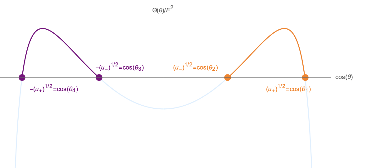
Figure 9. Plot of $\Theta(\theta)/E^{2}$ for $a=4,\mathcal{Q}=-2,|\Phi|=\sqrt{3}$. The $\theta$-motion is allowed in the orange region, above the equatorial hyperplane and in the purple region, below it.

The $\theta$-motion is allowed in the region where $\tilde{\Theta}(u)$ and hence $\Theta(\theta)/E^{2}$ are non-negative:

$$0<\theta_{1}\leq\theta\leq\theta_{2}<\pi/2\hskip 14.22636pt\textrm{in the orange region, above the}\;Eq,$$

$$\pi/2<\theta_{3}\leq\theta\leq\theta_{4}<\pi\hskip 14.22636pt\textrm{in the purple region, below the}\;Eq.$$

This $\theta$-motion is shown in Fig. 11 and the corresponding $\theta$-$\phi$-motion in Fig. 12.

If $0<u_{-}<u_{+}=1$, the graph of $\Theta(\theta)/E^{2}$ is shown in Fig. 10.

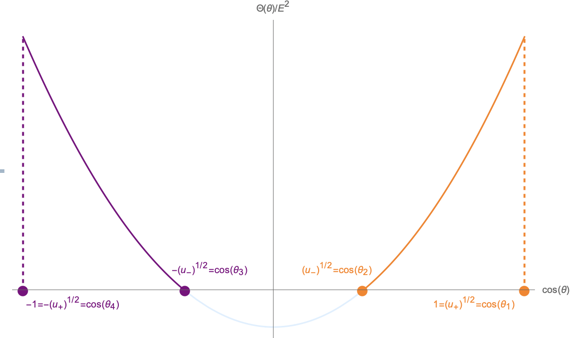
Figure 10. Plot of $\Theta(\theta)/E^{2}$ for $a=4,\mathcal{Q}=-2,\Phi=0$. The $\theta$-motion is allowed in the orange region, oscillating simmetrically around $\{\theta=0\}$ above the equatorial hyperplane and in the purple region, oscillating simmetrically around $\{\theta=\pi\}$ below the equatorial hyperplane.

These geodesics intersect the axis $A=\{\theta=0,\pi\}$ and hence $\Phi=0$ because $\tilde{\partial}_{\phi}=0$ on $A$. The $\theta$-motion is allowed where $\tilde{\Theta}(u)$ and hence $\Theta(\theta)/E^{2}$ are non-negative:

$$0=\theta_{1}\leq\theta\leq\theta_{2}<\pi/2\hskip 14.22636pt\textrm{in the orange region, above the}\;Eq,$$

$$\pi/2<\theta_{3}\leq\theta\leq\theta_{4}=\pi\hskip 14.22636pt\textrm{in the purple region, below the}\;Eq.$$

This $\theta$-motion is shown in Fig. 13 and the corresponding $\theta$-$\phi$-motion in Fig. 14.

There is a difference between the motions of Fig. 9 and Fig. 10. In the first case, the geodesics oscillates between $\theta_{1}$ and $\theta_{2}$ (or between $\theta_{3}$ and $\theta_{4}$), corresponding to half $\theta$-oscillation. In the second case instead, the geodesics complete symmetric oscillations around the axis, either above the equatorial hyperplane, crossing $\{\theta=0\}$ or below the equatorial hyperplane crossing $\{\theta=\pi\}$. However, the motion between $\theta_{1}=0$ and $\theta_{2}$ (or between $\theta_{3}$ and $\theta_{4}=\pi$) still corresponds to half $\theta$-oscillation (see Figures 13, 10 and Cor. $4.5.6$ in [35]).

In both oscillating cases, since $r=\textrm{const}$, (11) implies that the coordinate $\theta(s)$ oscillates periodically in the corresponding $\theta$-interval (see Figures 11 and 13). ∎

Consider the first order equations of motion (with the rescaled constants of motion $\mathcal{Q}:=Q/E^{2},\Phi:=L/E$), for a constant $r<0$:

(17) $$\frac{\rho^{2}(r,\theta)}{E}\frac{d\theta}{ds} =\pm\sqrt{\Theta(\theta)}=\pm\sqrt{\mathcal{Q}+a^{2}\cos^{2}\theta-\Phi^{2}\frac{\cos^{2}\theta}{\sin^{2}\theta}}$$

(18) $$\frac{\rho^{2}(r,\theta)}{E}\frac{dt}{ds} =\frac{r^{2}+a^{2}}{\Delta}(r^{2}+a^{2}-a\Phi)+a(\Phi-a\sin^{2}\theta).$$

Because of the $\theta$-differential equation, we can restrict to an interval $\mathcal{U}\subset\theta^{-1}\big{(}(\theta_{1},\theta_{2})\big{)}$ on which $d\theta/ds$ is either everywhere positive or everywhere negative (depending on the initial condition). Due to the symmetry in (17) and the fact that $r=\textrm{const}$, $\theta(s)$ is periodic over twice the interval $\mathcal{U}$. For instance, set $\mathcal{U}=(0,T/2)$, starting from $\theta(0)=\theta_{1}$, hence $\theta^{\prime}(s)=+\sqrt{\Theta(\theta)}>0$ for $s\in(0,T/2)$, then $\theta^{\prime}(s)=-\sqrt{\Theta(\theta)}<0$ for $s\in(T/2,T)$, where $\theta^{\prime}(T/2)=0$, because $\theta(T/2)=\theta_{2}$ (${}^{\prime}\equiv d/ds$) and Prop. 3.9, which explains the change of sign of $\theta^{\prime}(s)$ (using the fact that $\theta_{1},\theta_{2}$ are multiplicity one zeroes of $\Theta(\theta)$). Hence every $\Delta s=T/2$, $\theta^{\prime}(s)$ changes sign.

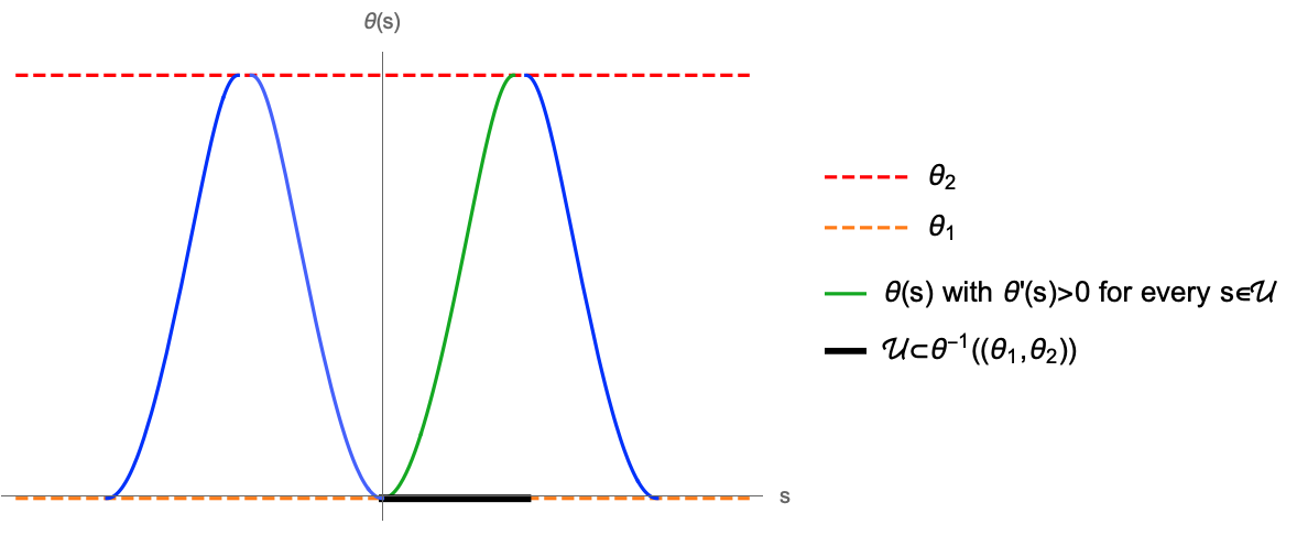
Figure 11. $\theta(s)$ obtained numerically from (17), with $a=3,M=8,\\ E=1,\mathcal{Q}=-1.252,\Phi=1.407$ and $r=-1$. The open subset $\mathcal{U}$ (black in the figure) is an interval on which $\theta(s)$ is strictly monotonic.

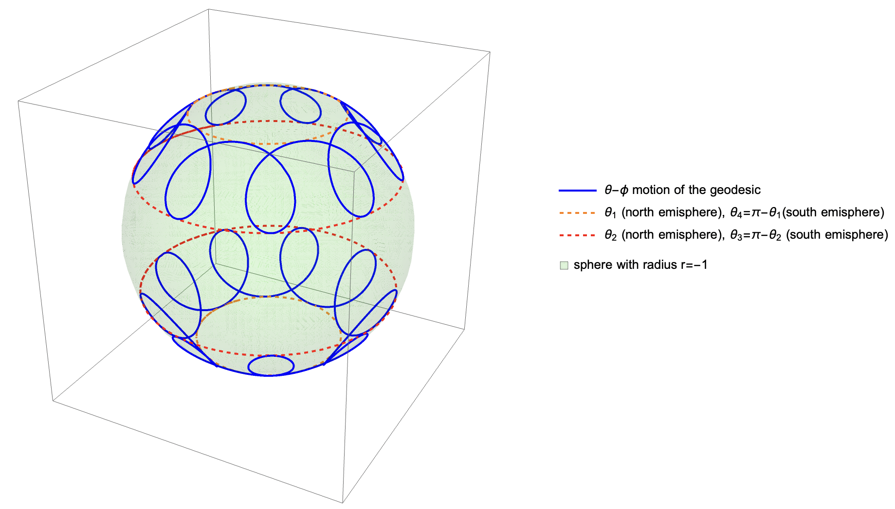
Figure 12. $\theta$-$\phi$ motion obtained numerically from the geodesic equations, with $a=3,M=8,E=1,\mathcal{Q}=-1.252,\Phi=1.407$ and $r=-1$ and initial conditions $\gamma(0)=(0,-1,\theta_{1},0),\;\gamma^{\prime}(0)\approx(0.529,0,0,0.376)$.

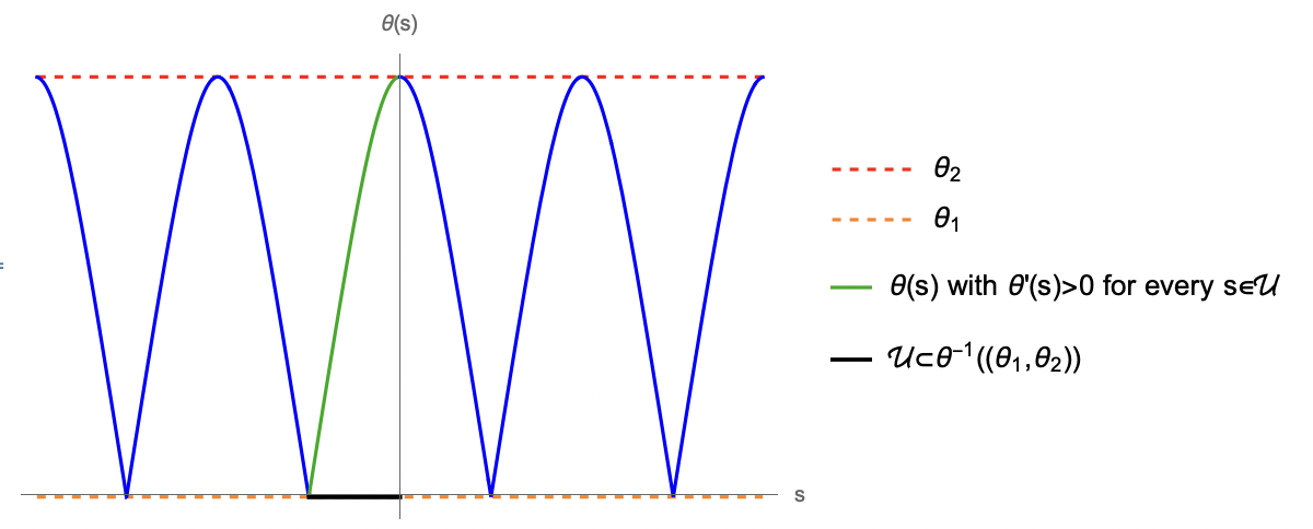
Figure 13. $\theta(s)$ obtained numerically from the geodesic equation with
$a=3,M=8,r=r_{\textrm{crit}}<0$ where $r_{\textrm{crit}}$ is the radius at which $\mathbf{g}(\partial_{\phi},\partial_{\phi})|_{r=r_{\textrm{crit}},\theta=\theta_{2}}=0$ and initial conditions $\gamma(0)=(0,r_{\textrm{crit}},\theta_{2},0)$ and $\gamma^{\prime}(0)=(0,0,0,-1)$. Hence, since $\gamma^{\prime}(0)=-\partial_{\phi}$, the geodesic has $\Phi=0$ ($L=0$). The Carter constant is set to $\mathcal{Q}=-5.409$. The open subset $\mathcal{U}$ (black in the figure) is an interval on which $\theta(s)$ is strictly monotonic.

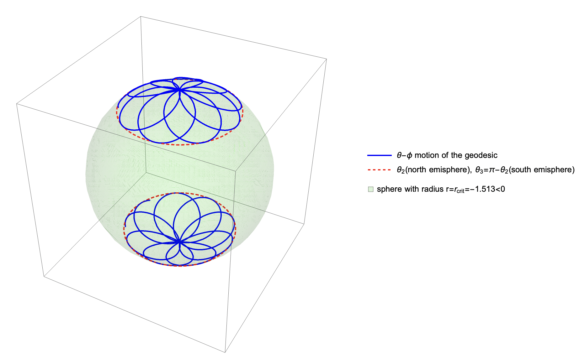
Figure 14. $\theta$-$\phi$ motion obtained numerically from the geodesic equation with
$a=3,M=8,r=r_{\textrm{crit}}<0,\mathcal{Q}=-5.409,\Phi=0$ where $r_{\textrm{crit}}$ is the radius at which $\mathbf{g}(\partial_{\phi},\partial_{\phi})|_{r=r_{\textrm{crit}},\theta=\theta_{2}}=0$ and initial conditions $\gamma(0)=(0,r_{\textrm{crit}},\theta_{2},0)$ and $\gamma^{\prime}(0)=(0,0,0,-1)$. Notice that the geodesic crosses $\theta_{1}=0$ and $\theta_{4}=\pi$ with non-zero velocity.

At parameters where $\Theta(\theta)\neq 0$ we can combine (18) and (17) to get

(19) $$\frac{dt}{d\theta}=\frac{r^{2}\Delta+2Mr(r^{2}+a^{2}-a\Phi)}{\pm\Delta\sqrt{\Theta(\theta)}}+a^{2}\frac{\cos^{2}\theta}{\pm\sqrt{\Theta(\theta)}}=B(r)\frac{1}{\pm\sqrt{\Theta(\theta)}}+a^{2}\frac{\cos^{2}\theta}{\pm\sqrt{\Theta(\theta)}},$$

with $B(r):=\frac{r^{2}\Delta+2Mr(r^{2}+a^{2}-a\Phi)}{\Delta}.$

Proposition 5.9 (See [10], [42]).

In a Kerr spacetime, a null geodesic with negative Carter constant $\mathcal{Q}$ and constant radial coordinate has the following pair of constants of motion

(20) $$\Phi=\Phi(r)=\frac{r^{2}(r-3M)+a^{2}(M+r)}{a(M-r)}\;,\hskip 28.45274pt\mathcal{Q}=\mathcal{Q}(r)=-r^{3}\frac{(r^{3}-6Mr^{2}+9M^{2}r-4a^{2}M)}{a^{2}(M-r)^{2}}.$$

Proof.

Since $E\neq 0$ by Prop. 4.5, we can divide the $r$-equation by $E^{2}$ to get

(21) $$\bigg{(}\frac{\rho^{2}}{E}\bigg{)}^{2}(r^{\prime})^{2}=r^{4}+(a^{2}-\Phi^{2}-\mathcal{Q})r^{2}+2M\bigg{(}(a-\Phi)^{2}+\mathcal{Q}\bigg{)}r-a^{2}\mathcal{Q}=:\mathcal{R}(r),$$

where $\Phi:=L/E$ and $\mathcal{Q}:=Q/E^{2}$. A geodesic has constant radial behaviour if and only if $\mathcal{R}(r)=0$ and $d\mathcal{R}(r)/dr=0$. These two equations can be solved for $\mathcal{Q}$ and $\Phi$. The two resulting pairs of constants of motion are (20) and

(22) $$\Phi=\Phi(r) =\frac{r^{2}+a^{2}}{a}\;,\hskip 104.70593pt\mathcal{Q}=\mathcal{Q}(r)=-\frac{r^{4}}{a^{2}},$$

where $r$ is the constant radius of the geodesic. Recall that $u_{-}+u_{+}=w/a^{2}>0$. However (22) implies

$$w=-2r^{2}<0.$$

Hence no null geodesic with constant radial coordinate and $\mathcal{Q}<0$ satisfies (22). ∎

The first integral $\Phi=\Phi(r)$ is given by (20). Hence $B(r)$ reduces to

(23) $$B(r)=\frac{r^{2}(3M+r)}{r-M}.$$

Remark 5.10.

Notice that if $B(r)\geq 0$, there would be nothing to prove. Indeed, in this case the $t$-coordinate would be non-decreasing, hence non-periodic. However $B(r)<0$ for a negative $r$ sufficiently close to zero. (In Fact, this holds for all spherical geodesics with $Q<0$, see Appendix B.) Moreover, numerical simulation shows that the $t$-component is not necessarily monotonic for a $Q<0$ geodesic with constant $r<0$ close to zero, see Fig. 15. Therefore we shall evaluate $\Delta t$ on a full $\theta$-oscillation.

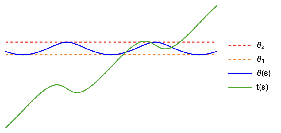
Figure 15. $\theta(s)$ obtained numerically from the geodesic equation with
$a=3,M=8,r=\bar{r}=-1<0$ and initial conditions $\gamma(0)=(0,\bar{r},\theta_{1},0)$ and $\gamma^{\prime}(0)=(1,0,0,0.710)$. Here $\mathcal{Q}=-1.252$ and $\Phi=1.407$.

We are now finally ready to rule out constant radius geodesics in the subcase $E\neq 0$, $Q<0$.

By contradiction, suppose there exists such a closed null geodesic $\gamma:I\rightarrow K^{*}$ with non-constant coordinate functions $s\mapsto t(s),\theta(s),\phi(s)$ and constant negative radial coordinate such that $B(r)<0$. The differential equation (19) has the form

$$\frac{dt}{d\theta}=F(\theta),$$

for some function $F$. The variation of the $t$-coordinate on a full $\theta$-oscillation is given by

$$\Delta t=2\int_{\theta_{1}}^{\theta_{2}}F(\theta)d\theta.$$

Remark 5.11.

Notice the factor $"2"$ in the last expression. On a full $\theta$-oscillation, we have

$$\int_{\theta_{1}}^{\theta_{2}}F(\theta)d\theta+\int_{\theta_{2}}^{\theta_{1}}-F(\theta)d\theta=2\int_{\theta_{1}}^{\theta_{2}}F(\theta)d\theta.$$

Therefore the variation of the $t$-coordinate after $n$ $\theta$-oscillations is $n\Delta t$ because of the periodicity of the $\theta$-coordinate. If the geodesic is closed, $\Delta t=0$, otherwise the coordinate $t(s)$ cannot be periodic. Hence it suffices to study what happens on a single $\theta$-oscillation.

Remark 5.12.

A motion of the kind $\pi\geq\theta_{4}\geq\theta\geq\theta_{3}>\pi/2$ produces the same integrals since in this $\theta$-interval $\cos\theta<0$, hence with the substitution $u=\cos^{2}\theta$ we have $d\theta=\frac{1}{2}\frac{du}{\sqrt{u}\sqrt{1-u}}$. Therefore

$$\int_{\theta_{1}}^{\theta_{2}}\frac{d\theta}{\sqrt{\Theta(\theta)}}=\int_{\theta_{3}}^{\theta_{4}}\frac{d\theta}{\sqrt{\Theta(\theta)}},\hskip 28.45274pt\int_{\theta_{1}}^{\theta_{2}}\frac{\cos^{2}\theta\;d\theta}{\sqrt{\Theta(\theta)}}=\int_{\theta_{3}}^{\theta_{4}}\frac{\cos^{2}\theta\;d\theta}{\sqrt{\Theta(\theta)}}.$$

Hence $\Delta t$ is the same.

So without any loss of generality, we may consider a motion of the type $0\leq\theta_{1}\leq\theta\leq\theta_{2}<\pi/2$. Then we can integrate (19) on a full oscillation to get

(24) $$\Delta t=2B(r)\int_{\theta_{1}}^{\theta_{2}}\frac{d\theta}{\sqrt{\Theta(\theta)}}+2a^{2}\int_{\theta_{1}}^{\theta_{2}}\frac{cos^{2}\theta\;d\theta}{\sqrt{\Theta(\theta)}}.$$

We now have to compute the following integrals

$$I_{1}:= \int_{\theta_{1}}^{\theta_{2}}\frac{d\theta}{\sqrt{\Theta(\theta)}},$$

$$I_{2}:= \int_{\theta_{1}}^{\theta_{2}}\frac{\cos^{2}\theta\;d\theta}{\sqrt{\Theta(\theta)}}.$$

Let us start from the first integral:

(25) $$I_{1}=-\frac{1}{2}\int_{u_{+}}^{u_{-}}\frac{du}{\sqrt{u}\sqrt{\tilde{\Theta}(u)}},$$

where we have used the substitution $u:=\cos^{2}\theta$, hence $d\theta=-\frac{1}{2}\frac{du}{\sqrt{u}\sqrt{1-u}}$ since
$\sin\theta\geq 0$ and $\cos\theta>0$ if $\theta_{1}\leq\theta\leq\theta_{2}$. Now we can use (11) and the substitution
$u=:u_{-}+(u_{+}-u_{-})y^{2}$ adopted in [26] to get

$$I_{1}= \frac{1}{2}\int_{u_{-}}^{u_{+}}\frac{du}{\sqrt{u}\sqrt{a^{2}(u_{+}-u)(u-u_{-})}}$$

$$= \frac{1}{2|a|}\int_{0}^{1}\frac{2(u_{+}-u_{-})ydy}{\sqrt{u_{-}+(u_{+}-u_{-})y^{2}}\sqrt{\big{(}u_{+}-u_{-}-(u_{+}-u_{-})y^{2}\big{)}(u_{+}-u_{-})y^{2}}}$$

$$= \frac{1}{|a|}\int_{0}^{1}\frac{dy}{\sqrt{u_{-}+(u_{+}-u_{-})y^{2}}\sqrt{1-y^{2}}}$$

$$= \frac{1}{|a|\sqrt{u_{-}}}\int_{0}^{1}\frac{dy}{\sqrt{1-y^{2}}\sqrt{1-\big{(}1-\frac{u_{+}}{u_{-}}\big{)}y^{2}}}.$$

With the same substitutions, we also get

$$I_{2}= -\frac{1}{2}\int_{u_{+}}^{u_{-}}\frac{udu}{\sqrt{u}\sqrt{\tilde{\Theta}(u)}}$$

$$= \frac{1}{2}\int_{u_{-}}^{u_{+}}\frac{udu}{\sqrt{u}\sqrt{a^{2}(u_{+}-u)(u-u_{-})}}$$

$$= \frac{1}{|a|}\int_{0}^{1}\frac{\sqrt{u_{-}+(u_{+}-u_{-})y^{2}}}{\sqrt{1-y^{2}}}dy$$

$$= \frac{\sqrt{u_{-}}}{|a|}\int_{0}^{1}\frac{\sqrt{1-\big{(}1-\frac{u_{+}}{u_{-}}\big{)}y^{2}}}{\sqrt{1-y^{2}}}dy.$$

Then with the definition of the elliptic integrals in Appendix A we have

(26) $$I_{1}= \frac{1}{|a|\sqrt{u_{-}}}\mathcal{K}\bigg{(}1-\frac{u_{+}}{u_{-}}\bigg{)},$$

(27) $$I_{2}= \frac{\sqrt{u_{-}}}{|a|}\mathcal{E}\bigg{(}1-\frac{u_{+}}{u_{-}}\bigg{)}.$$

Hence, we get

(28) $$\Delta t=\frac{2B(r)}{|a|\sqrt{u_{-}}}\mathcal{K}\bigg{(}1-\frac{u_{+}}{u_{-}}\bigg{)}+2|a|\sqrt{u_{-}}\mathcal{E}\bigg{(}1-\frac{u_{+}}{u_{-}}\bigg{)}.$$

Note that, since $u_{+}>u_{-}>0$, we have $1-\frac{u_{+}}{u_{-}}<0$, and hence $\mathcal{E}(1-u_{+}/u_{-})>\mathcal{K}(1-u_{+}/u_{-})>0$ (see Appendix A). However, the prefactor of $\mathcal{E}$ does not dominate the opposite of the prefactor of $\mathcal{K}$ for every negative $r$, as one may check substituting $\Phi(r)$ and $\mathcal{Q}(r)$ from (20) into $u_{-}$ given by (12).

From now on set $x:=1-u_{+}/u_{-}$. The elliptic integral $\mathcal{K}$ can be written as a hypergeometric function (see A.5):

$$\mathcal{K}(x)=\frac{\pi}{2}F\bigg{(}\frac{1}{2},\frac{1}{2};1;x\bigg{)}.$$

Using the Pfaff transformation (see A.6)

(29) $$F\bigg{(}\alpha,\beta;\gamma;x\bigg{)}=(1-x)^{-\alpha}F\bigg{(}\alpha,\gamma-\beta;\gamma;\frac{x}{x-1}\bigg{)},$$

we can decrease the modulus of the prefactor in front of the elliptic integral $\mathcal{K}$:

(30) $$\mathcal{K}(x)=\frac{\sqrt{u_{-}}}{\sqrt{u_{+}}}\mathcal{K}\bigg{(}\frac{x}{x-1}\bigg{)}.$$

Hence we get

(31) $$\Delta t=2|a|\sqrt{u_{-}}\mathcal{E}(x)+\frac{2B(r)}{|a|\sqrt{u_{+}}}\mathcal{K}\bigg{(}\frac{x}{x-1}\bigg{)}.$$

Now we compare the elliptic integrals, after the Pfaff transformation. Since $x<0$, we have

(32) $$\mathcal{E}(x)>\mathcal{K}\bigg{(}\frac{x}{x-1}\bigg{)}>0,$$

by Rmk. A.2. Next we claim that the prefactors of the elliptic integrals in (31) satisfy

(33) $$2|a|\sqrt{u_{-}}>-\frac{2B(r)}{|a|\sqrt{u_{+}}}.$$

Indeed, both sides of the inequality are positive, so we can square them and use that $u_{+}u_{-}=-\mathcal{Q}(r)/a^{2}$ by (11) to get an equivalent inequality

$$-\mathcal{Q}(r)a^{2}>B^{2}(r),$$

where $\mathcal{Q}(r)$ is given by (20) and $B(r)$ by (23) , or equivalently

$$(-12Mr^{2}-4a^{2}M)r>0.$$

This last inequality is clearly satisfied in $r<0$. Combining (31), (32) and (33), we conclude that $\Delta t>0$ for all $r<0$, which shows that the spherical geodesics cannot be closed.

In Fig. 16 we see the plot of $\Delta t$ given by (31) as function of the fixed radius $r$ after the substitutions of $\Phi(r)$ and $\mathcal{Q}(r)$ from (20) into $u_{\pm}$ given by (12).

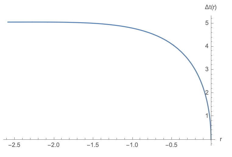
Figure 16. Plot of $\Delta t=\Delta t(r)$ for $r<0$ close to zero with $a=5,\,M=7$.

We have ruled out all the possibilities on Fig. 3, therefore there are no closed null geodesics in the Kerr-star spacetime.

Appendix A Elliptic integrals and hypergeometric functions

Definition A.1.

Let $\phi\in[-\pi/2,\pi/2]$. The elliptic integral of the first kind is

$$\mathcal{F}(\phi|k):=\int_{0}^{\sin\phi}\frac{ds}{\sqrt{(1-s^{2})(1-ks^{2})}}.$$

The complete $(\phi=\pi/2)$ elliptic integral of the first kind is

$$\mathcal{K}(k):=\mathcal{F}(\pi/2|k)=\int_{0}^{1}\frac{ds}{\sqrt{(1-s^{2})(1-ks^{2})}}.$$

The elliptic integral of the second kind is

$$\mathcal{E}(\phi|k):=\int_{0}^{\sin\phi}\sqrt{\frac{1-ks^{2}}{1-s^{2}}}ds.$$

The complete $(\phi=\pi/2)$ elliptic integral of the second kind is

$$\mathcal{E}(k):=\mathcal{E}(\pi/2|k)=\int_{0}^{1}\sqrt{\frac{1-ks^{2}}{1-s^{2}}}ds.$$

We define also

$$\mathcal{D}(k):=\int_{0}^{1}\frac{s^{2}ds}{\sqrt{(1-s^{2})(1-ks^{2})}}=\frac{\mathcal{K}(k)-\mathcal{E}(k)}{k}=-2\frac{\partial\mathcal{E}(k)}{\partial k}.$$

Remark A.2.

Let $0<z,s<1,\;x<0$.

$$\sqrt{\frac{1-zs^{2}}{1-s^{2}}}>\frac{1}{\sqrt{1-s^{2}}\sqrt{1-xs^{2}}}\hskip 14.22636pt\Longleftrightarrow\hskip 14.22636pt(1-zs^{2})(1-xs^{2})>1\hskip 14.22636pt\Longrightarrow\hskip 14.22636pt\mathcal{E}(x)>\mathcal{K}(z).$$

If $z=x/(x-1)$, it satisfies $0<z<1$ and we have

$$(1-zs^{2})(1-xs^{2})>1\hskip 14.22636pt\Longleftrightarrow\hskip 14.22636ptx+z<xzs^{2}\hskip 14.22636pt\Longleftrightarrow\hskip 14.22636pt1>s^{2},$$

hence $\mathcal{E}(x)>\mathcal{K}(z)$.

Definition A.3 ([1]).

The hypergeometric function $F(\alpha,\beta;\gamma;x)$ is defined by the series

$$\sum_{n=0}^{\infty}\frac{(\alpha)_{n}(\beta)_{n}}{(\gamma)_{n}n!}x^{n},$$

where $(\alpha)_{n}:=\alpha(\alpha+1)\cdot...\,\cdot(\alpha+n-1)$ for $n>0$, $(\alpha)_{0}\equiv 1$ (analogous for the others), for $|x|<1$, and by continuation elsewhere.

Proposition A.4 (Euler’s integral representation, see [1]).

If $\textrm{Re}\;\gamma>\textrm{Re}\;\beta>0$, then

$$F(\alpha,\beta;\gamma;x)=\frac{\Gamma(\gamma)}{\Gamma(\beta)\Gamma(\gamma-\beta)}\int_{0}^{1}t^{\beta-1}(1-t)^{\gamma-\beta-1}(1-xt)^{-\alpha}dt$$

in the complex $x-$plane cut along the real axis from $1$ to $+\infty$, where $\Gamma(x):=\int_{0}^{\infty}t^{x-1}e^{-t}dt$ is the Euler’s gamma function.

Proposition A.5 ([1]).

We can write the complete elliptic integral of the first kind as

$$\mathcal{K}(x)=\frac{\pi}{2}F\bigg{(}\frac{1}{2},\frac{1}{2};1;x\bigg{)}.$$

Proof.

Use the integral representation of the hypergometric function given in Prop. A.4, the integral substitution $t=s^{2}$, with $\Gamma(\frac{1}{2})=\sqrt{\pi}$, $\Gamma(1)=1$. ∎

Proposition A.6 (”Pfaff’s formula”, see Theorem $2.2.5$ of [1]).

$$F(\alpha,\beta;\gamma;x)=(1-x)^{-\alpha}F\bigg{(}\alpha,\gamma-\beta;\gamma;\frac{x}{x-1}\bigg{)}.$$

Proof.

Use A.4 and the integral substitution $t=1-s$. ∎

Appendix B Spherical null geodesics with $Q<0$

Proposition B.1.

In the Kerr-star spacetime $K^{*}$, null geodesics with constant radial coordinate and $\mathcal{Q}<0$ exist if and only if $r\in\big{[}R_{2}(a,M),0\big{)}$, where $R_{2}(a,M)$ is given by (35).

Proof.

($\Rightarrow$) Consider (11). We must have $\tilde{\Theta}(u)\geq 0$, hence $\textrm{dis}:=w^{2}+4a^{2}\mathcal{Q}\geq 0$, where $w:=a^{2}-\Phi^{2}-\mathcal{Q}$. We know that for spherical geodesics $\Phi$ and $\mathcal{Q}$ are given by (20). Therefore we have

(34) $$\textrm{dis}=\frac{16Mr^{2}}{(M-r)^{4}}\Delta(r)(2r^{3}-3Mr^{2}+a^{2}M)=:\frac{16Mr^{2}}{(M-r)^{4}}\Delta(r)k(r)\geq 0.$$

Since $\Delta(r)>0$ for negative $r$, the last inequality is equivalent to $k(r)\geq 0$. The signs of the coefficients of $k(r)$ are $+\;-\;+$, hence either there are two or zero positive roots. But the sum of the roots is $3M/2>0$, hence there are two positive roots. Moreover $k(0)=a^{2}M>0$ and $\lim_{x\rightarrow-\infty}k(r)=-\infty$, hence the third root is negative. These roots can be expressed in the following way (see [48])

(35) $$R_{j}(a,M)=M\cos\bigg{[}\frac{1}{3}\arccos\bigg{(}1-2\frac{a^{2}}{M^{2}}\bigg{)}-\frac{2}{3}j\pi\bigg{]}+\frac{M}{2}\hskip 28.45274ptj=0,1,2,$$

with $R_{2}(a,M)<0<R_{1}(a,M)<R_{0}(a,M)$.

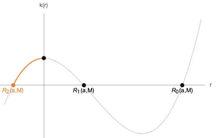
Figure 17. Plot of $k(r)$ for $a=3,M=5$.

Hence (34) can only be satisfied for $r\in\big{[}R_{2}(a,M),0\big{)}$.

($\Leftarrow$) Assume first that $r=r_{0}\in\big{(}R_{2}(a,M),0\big{)}$ and fix $\Phi=\Phi(r_{0})$, $\mathcal{Q}=\mathcal{Q}(r_{0})$ by (20) so that

(36) $$\textrm{dis}=w^{2}(r_{0})+4a^{2}\mathcal{Q}(r_{0})=[\mathcal{Q}(r_{0})+(|\Phi(r_{0})|-|a|)^{2}][\mathcal{Q}(r_{0})+(|\Phi(r_{0})|+|a|)^{2}]>0,$$

with $w(r):=a^{2}-\Phi^{2}(r)-\mathcal{Q}(r)$. Notice that $[\mathcal{Q}(r)+(|\Phi(r)|+|a|)^{2}]\geq[\mathcal{Q}(r)+(\Phi(r)-a)^{2}]=4r^{2}\Delta(r)/(M-r)^{2}>0$ since $\Delta(r)>0$ for $r<0$. Therefore (36) implies that $[\mathcal{Q}(r_{0})+(|\Phi(r_{0})|-|a|)^{2}]>0$. Since $r_{0}\in\big{(}R_{2}(a,M),0\big{)}$, we have $\mathcal{Q}=\mathcal{Q}(r_{0})<0$ by (20) and $w(r_{0})>0$. Indeed the inequality takes the form

$$w(r_{0})=a^{2}-\Phi^{2}(r_{0})-\mathcal{Q}(r_{0})=-2r_{0}\frac{r^{3}_{0}-3M^{2}r_{0}+2a^{2}M}{(M-r_{0})^{2}}>0.$$

This inequality is automatically satisfied for $r_{0}\in(R_{2}(a,M),0)$, since $r_{0}^{3}-3M^{2}r_{0}\geq 0$ for $r_{0}\in[-\sqrt{3}M,0)$ and $-\sqrt{3}M<-M/2\leq R_{2}(a,M)$ by (35).

Using (12) we have then

$$0<u_{-}:=\frac{w(r_{0})-\sqrt{w^{2}(r_{0})+4a^{2}\mathcal{Q}(r_{0})}}{2a^{2}}<\frac{w(r_{0})}{2a^{2}}<\frac{a^{2}-\Phi(r_{0})^{2}+(|\Phi(r_{0})|-|a|)^{2}}{2a^{2}}=1-\frac{|\Phi(r_{0})|}{|a|}\leq 1,$$

so that we can define $\theta_{2}:=\arccos(\sqrt{u_{-}})\in(0,\pi)$. We now fix the initial point $p_{0}=(0,r_{0},\theta_{0},0)\in K^{*}$ with $\theta_{0}:=\theta_{2}$, $r_{0}\in(R_{2}(a,M),0)$ and the following set of constants of motion $(q=0,E=1,L=\Phi(r_{0}),K=\mathcal{Q}(r_{0})+(\Phi(r_{0})-a)^{2})$ by (20). Then $\Theta(\theta_{0})=0$ by (11) and $R(r_{0})=0$ by (20).

By Prop. $4.2.6$ in [35], there exists a null geodesic starting at $p_{0}$ with that particular set of constants of motion.

Assume now $r=R_{2}(a,M)$. Choose a converging sequence of initial points $p_{n}=(0,r_{n},\theta_{n},0)\in K^{*}$ with $(R_{2}(a,M),0)\ni r_{n}\rightarrow R_{2}(a,M)$, $\theta_{n}:=\arccos(\sqrt{u_{-}(r_{n})})\in(0,\pi)$ with

$$u_{-}(r):=\frac{w(r)-\sqrt{w^{2}(r)+4a^{2}\mathcal{Q}(r)}}{2a^{2}},$$

and consider the corresponding geodesic $\gamma_{n}$ constructed above. The constants of motion of $\gamma_{n}$ converge and hence so do the tangent vectors $\gamma^{\prime}_{n}(p_{n})$ by (5). By continuity, there exists a geodesic $\gamma=\lim\gamma_{n}$ with $\mathcal{Q}=\mathcal{Q}[R_{2}(a,M)]<0$ by (20), starting at the point $p_{0}=(0,R_{2}(a,M),\arccos\bigg{(}\sqrt{u_{-}[R_{2}(a,M)]}\bigg{)},0)$ with $(q=0,E=1,L=\Phi[R_{2}(a,M)],K=\mathcal{Q}[R_{2}(a,M)]+[\Phi(R_{2}(a,M))-a]^{2})$ as constants of motion. The limit geodesic has constant $\theta$-coordinate and falls in the class described in Prop. 5.6. ∎

Remark B.2.

Note that $R_{2}(a,M)\geq-M/2$, so $B(r)<0$ by (23) for all geodesics of this type.

References

- [1] Andrews, G. E., Askey, R., and Roy, R. Special Functions. Encyclopedia of Mathematics and its Applications. Cambridge University Press, 1999.
- [2] Beem, J.K. and Ehrlich, P.E. and Easley, K.L. Global Lorentzian Geometry. Monographs and textbooks in pure and applied mathematics. Dekker, 1996.
- [3] Boyer, R. H., and Lindquist, R. W. Maximal analytic extension of the Kerr metric. Journal of Mathematical Physics 8, 2 (Feb. 1967), 265–281.
- [4] Boyer, R. H., and Price, T. G. An interpretation of the kerr metric in general relativity. Mathematical Proceedings of the Cambridge Philosophical Society 61, 2 (1965), 531–534.
- [5] Bronzwaer, T., and Falcke, H. The nature of black hole shadows. The Astrophysical Journal 920, 2 (oct 2021), 155.
- [6] B. P. Abbott et al. (LIGO Scientific Collaboration and Virgo Collaboration). Observation of gravitational waves from a binary black hole merger. Phys. Rev. Lett. 116 (Feb 2016), 061102.
- [7] Calvani, M., de Felice, F., Muchotrzeb, B., and Salmistraro, F. Time machine and geodesic motion in Kerr metric. Gen. Rel. Grav. 9 (1978), 155–163.
- [8] Carter, B. Complete analytic extension of the symmetry axis of Kerr’s solution of Einstein’s equations. Phys. Rev. 141 (Jan 1966), 1242–1247.
- [9] Carter, B. Global structure of the Kerr family of gravitational fields. Phys. Rev. 174 (Oct 1968), 1559–1571.
- [10] Chandrasekhar, S. The mathematical theory of black holes. 1983.
- [11] Chandrasekhar, S., and Wright, J. P. The geodesics in Gödel’S universe. Proceedings of the National Academy of Sciences of the United States of America 47 3 (1961), 341–7.
- [12] Chernov, V., and Nemirovski, S. Legendrian links, causality, and the Low conjecture. Geometric and Functional Analysis 19 (2009).
- [13] Chernov, V., and Nemirovski, S. Universal orderability of Legendrian isotopy classes. Journal of Symplectic Geometry 14, 1 (2016), 149–170.
- [14] Chernov, V. and Nemirovski, S. Non-negative Legendrian isotopy in . Geom.Topol. 14, 1 (2010), 611 – 626.
- [15] Chruściel, P., Maliborski, M., and Yunes, N. Structure of the singular ring in kerr-like metrics. Phys. Rev. D 101 (May 2020), 104048.
- [16] de Felice, F. Equatorial geodesic motion in the gravitational field of a rotating source. Nuovo Cim. B 57 (1968), 351.
- [17] de Felice, F., and Calvani, M. Causality violation in the Kerr metric. Gen. Rel. Grav. 10 (1979), 335–342.
- [18] Event Horizon Telescope Collaboration, Akiyama, K., Alberdi, A., et al. First M87 Event Horizon Telescope Results. I. The Shadow of the Supermassive Black Hole. The Astrophysical Journal Letters 875, 1 (apr 2019), L1.
- [19] Frolov, V., and Zelnikov, A. Introduction to Black Hole Physics. OUP Oxford, 2011.
- [20] Gödel, K. An Example of a New Type of Cosmological Solutions of Einstein’s Field Equations of Gravitation. Rev. Mod. Phys. 21 (Jul 1949), 447–450.
- [21] Gott, J. R. Closed timelike curves produced by pairs of moving cosmic strings: exact solutions. Phys. Rev. Lett. 66 (Mar 1991), 1126–1129.
- [22] Guillemin, V. Cosmology in (2 + 1) -Dimensions, Cyclic Models, and Deformations of M2,1. (AM-121). Princeton University Press, 1989.
- [23] Hawking, S. W. Chronology protection conjecture. Phys. Rev. D 46 (Jul 1992), 603–611.
- [24] Hawking, S. W., and Ellis, G. F. R. The Large Scale Structure of Space-Time. Cambridge Monographs on Mathematical Physics. Cambridge University Press, 1973.
- [25] Hedicke, J. and Suhr, S. Conformally Embedded Spacetimes and the Space of Null Geodesics. Communications in Mathematical Physics 375, 2 (2020), 1561–1577.
- [26] Kapec, D., and Lupsasca, A. Particle motion near high-spin black holes. Classical and Quantum Gravity 37, 1 (dec 2019), 015006.
- [27] Kerr, R. P. Gravitational field of a spinning mass as an example of algebraically special metrics. Phys. Rev. Lett. 11 (Sep 1963), 237–238.
- [28] Kundt, V. W. Trägheitsbahnen in einem von Gödel angegebenen kosmologischen Modell. Zeitschrift für Physik 145 (1956), 611–620.
- [29] Landsman,K. Foundations of General Relativity: From Einstein to Black Holes. Radboud University Press, 2021.
- [30] Li, L.-X. New light on time machines: against the chronology protection conjecture. Phys. Rev. D 50 (Nov 1994), R6037–R6040.
- [31] Low, R. Time machines without closed causal geodesics. Classical and Quantum Gravity 12, 5 (may 1995), L37.
- [32] Low, R. The space of null geodesics. Nonlinear Analysis: Theory, Methods & Applications 47, 5 (2001), 3005–3017. Proceedings of the Third World Congress of Nonlinear Analysts.
- [33] Low, R. J. The geometry of the space of null geodesics. Journal of Mathematical Physics 30, 4 (1989), 809–811.
- [34] Nolan, B. Causality violation without time-travel: closed lightlike paths in Gödel’s universe. Classical and Quantum Gravity 37, 8 (mar 2020), 085007.
- [35] O’Neill, B. The geometry of Kerr black holes. Ak Peters Series. Taylor & Francis, 1995.
- [36] Penrose, R. Twistor quantization and curved space-time. Int. J. Theor. Phys. 1 (1968), 61–99.
- [37] Penrose, R. Naked singularities. Annals of the New York Academy of Sciences 224, 1 (1973), 125–134.
- [38] Penrose, R. Techniques of Differential Topology in Relativity. CBMS-NSF Regional Conference Series in Applied Mathematics. Society for Industrial and Applied Mathematics, 1972.
- [39] Schwarzschild, K. Über das Gravitationsfeld eines Massenpunktes nach der Einsteinschen Theorie. Sitzungsberichte der Königlich Preussischen Akademie der Wissenschaften (Jan. 1916), 189–196.
- [40] Steadman, B. R. Letter: Causality Violation on van Stockum Geodesics. General Relativity and Gravitation 35 (2003), 1721–1726.
- [41] Suhr, S. A Counterexample to Guillemin’s Zollfrei Conjecture. Journal of Topology and Analysis 05, 03 (aug 2013), 251–260.
- [42] Teo, E. Spherical photon orbits around a Kerr black hole. General Relativity and Gravitation 35, 11 (2003).
- [43] Tipler, F. J. Rotating cylinders and the possibility of global causality violation. Phys. Rev. D 9 (Apr 1974), 2203–2206.
- [44] van Stockum, W. IX.—The gravitational gield of a distribution of particles rotating about an axis of symmetry. Proceedings of the Royal Society of Edinburgh 57.
- [45] Wald, R. General Relativity. Chicago Univ. Pr., Chicago, USA, 1984.
- [46] Walker, M., and Penrose, R. On quadratic first integrals of the geodesic equations for type spacetimes. Commun. Math. Phys. 18 (1970), 265–274.
- [47] Wilkins, D. Bound geodesics in the kerr metric. Phys. Rev. D 5 (Feb 1972), 814–822.
- [48] Zwillinger, D. CRC Standard Mathematical Tables and Formulae. Discrete mathematics and its applications. CRC Press, 2012.