GeoDTR+: Toward generic cross-view geolocalization via geometric disentanglement

Abstract

Cross-View Geo-Localization (CVGL) estimates the location of a ground image by matching it to a geo-tagged aerial image in a database. Recent works achieve outstanding progress on CVGL benchmarks. However, existing methods still suffer from poor performance in cross-area evaluation, in which the training and testing data are captured from completely distinct areas. We attribute this deficiency to the lack of ability to extract the geometric layout of visual features and models’ overfitting to low-level details. Our preliminary work [1] introduced a Geometric Layout Extractor (GLE) to capture the geometric layout from input features. However, the previous GLE does not fully exploit information in the input feature. In this work, we propose GeoDTR+ with an enhanced GLE module that better models the correlations among visual features. To fully explore the LS techniques from our preliminary work, we further propose Contrastive Hard Samples Generation (CHSG) to facilitate model training. Extensive experiments show that GeoDTR+ achieves state-of-the-art (SOTA) results in cross-area evaluation on CVUSA [2], CVACT [3], and VIGOR [4] by a large margin ($16.44\%$, $22.71\%$, and $17.02\%$ without polar transformation) while keeping the same-area performance comparable to existing SOTA. Moreover, we provide detailed analyses of GeoDTR+.

I Introduction

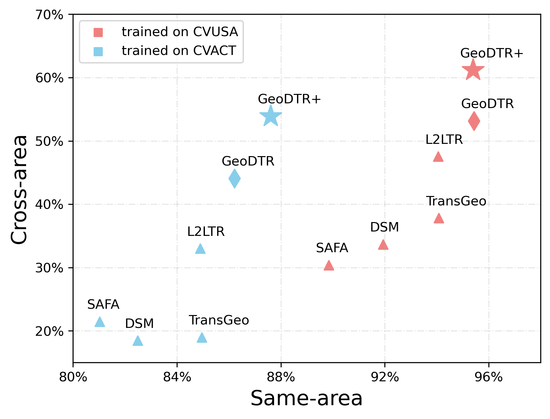
Figure 1: Comparison of R@$1$ accuracy between four recently published CVGL methods, including SAFA [5], DSM [6], TransGeo [7], L2LTR [8], GeoDTR [1], and our proposed GeoDTR+ on same-area performance (x axis) and cross-area performance (y axis). Notice that our preliminary work GeoDTR achieves the SOTA same-area and cross-area performance. In this work, built upon the GeoDTR, the proposed GeoDTR+ further improves more, especially on cross-area performance.

Estimating the location of a ground image from a database of geo-tagged aerial images, named “Cross-View Geo-Localization (CVGL)”, is one of the fundamental tasks that lies at the border of remote sensing and computer vision. The ground image is referred to as the query image and the geo-tagged aerial images are known as reference images. Different from same-view geo-localization which utilizes a geo-tagged ground images database for referencing, CVGL takes aerial images as reference data that is more accessible [9]. CVGL facilitates various tasks such as autonomous driving [10], unmanned aerial vehicle navigation [11], object localization [12], and augmented reality [13] by providing more accurate location estimation under certain environments. Existing approaches typically treat CVGL as an image retrieval problem [9]. This process extracts features from both ground and aerial images by either handcrafted descriptors or learned neural networks. The estimated location is the center of the aerial image which has the most similar feature to the query image in latent space [5, 6, 8, 14, 15, 2, 16, 17, 3, 18, 19]. To achieve this goal, these methods normally train a model to push the corresponding aerial image and ground image pairs (also known as aerial-ground pairs) closer in latent space and push the unmatched pairs further away from each other.

CVGL is considered an extremely challenging problem because of: (i) the drastic difference in the viewing angles between ground and aerial images, (ii) the huge variance in capturing time of both ground and aerial images, (iii) very different resolutions between ground and aerial images. Addressing such challenges requires a comprehensive and profound understanding of the image content and the spatial configuration (i.e. the relative locations between each landmark in an image). Most existing methods [5, 14, 20, 17, 21, 15] pair the query ground image and reference image by exploiting features extracted by Convolutional Neural Networks (CNNs). For example, Spatial-Aware Feature Aggregation (SAFA) [5] proposed to explore the CNN extracted feature by a customized Spatial-aware Positional Embedding (SPE) module. Such methods are limited in exploring the spatial configuration which is a global property (i.e. a highway spanning west to east on an aerial image) due to the tendency to explore local correlations among pixels in CNNs. Recently, transformer [22] has been introduced in CVGL [8, 7, 23] to capture the global contextual information. Nevertheless, in these methods, the spatial configuration is unavoidably entangled with low-level features because the multi-head attention mechanism implicitly models those correlations.

Typically, CVGL models are expected to generalize on unseen data with minimal supervision, for example, estimating the locations of autonomous vehicles or smartphones at any geospatial point. Furthermore, popular CVGL methods heavily rely on a certain area with high-quality aerial-ground image pairs for effective training, which is not always accessible at other locations. Consequently, there is a pressing need to develop generalizable CVGL algorithms capable of estimating the location of ground query data from any geographic area which is also known as cross-area evaluation (i.e. training and testing on two distinct geographic areas). Despite the evaluation of existing CVGL algorithms on datasets where the training and testing data originate from both the same geographical area (same-area) and different geographical locations (cross-area), the current emphasis within the CVGL field is primarily placed on improving same-area performance [5, 14, 6]. This results in a significant performance gap between same-area and cross-area performance and a lack of focus on achieving satisfactory cross-area performance. For example, as shown in Figure 1, on CVUSA [2] dataset, SAFA [5], L2LTR [8], DSM [6], and TransGeo [7] achieve around $90\%$ R@$1$ accuracy on same-area evaluation but only achieve $30\%$ to $40\%$ R@$1$ accuracy on cross-area performance. Furthermore, on CVACT [3] dataset, these methods can only achieve $20\%$ to $30\%$ R@$1$ accuracy on cross-area performance while achieving more than $80\%$ R@$1$ accuracy on same-area performance.

As demonstrated in Figure 1, there is a notable gap between the same-area and the cross-area performance of these algorithms. This paper seeks to answer the question - how to generalize cross-view geo-localization algorithms with minimal supervision?

A preliminary version of this work has been published at the 37th AAAI conference on artificial intelligence [1]. In that work, we proposed a Geometric Layout Extractor (GLE) module to capture spatial configuration, as well as Layout simulation and Semantic augmentation (LS) techniques to diversify the training data. Moreover, a counterfactual (CF) learning schema was introduced to provide additional supervision for the geometric layout extractor module. However, the proposed GLE module only explores geometric correlations within a learned subspace, which may result in a loss of information. Additionally, the effectiveness of the proposed LS techniques in enhancing cross-area performance remains limited, as they were only utilized in a data augmentation manner in the preliminary work. To address the above-mentioned limitations, this work extends the previous study in the following three aspects. First, we improve the design of the geometric layout extractor module to better capture the spatial configurations in both aerial and ground images (Section III-C2). Second, in our previous work, LS techniques are adopted as a special data augmentation that implicitly introduces inter-batch contrastive signals for layout and semantic features. Inspired by the hard sample mining strategy in cross-view geo-localization [4], we extend LS techniques to explicitly include intra-batch contrastive signals in the current work (Section III-E). In this way, our GeoDTR+ is expected to distinguish these “generated hard” samples in a single batch. We named this process the “Contrastive Hard Samples Generation” (CHSG) procedure. By integrating CHSG with the novel geometric layout extractor, GeoDTR+ is able to learn better latent representations explicitly from generated hard samples within a single batch. This results in a substantial improvement in cross-area performance compared to the current state-of-the-art (SOTA) methods. Furthermore, we provide more comprehensive benchmark results of GeoDTR+ with other CVGL methods on more challenging datasets [4] and also provide additional analyses (Section IV) and visualizations examples. Our contribution to this paper can be summarized as threefold,

• We present Geometric Descriptor TRansformer plus (GeoDTR+), a novel CVGL model that is built upon our preliminary GeoDTR [1] model. GeoDTR+ can effectively model the spatial configuration of both ground and aerial images through the proposed novel geometric layout extraction mechanism.

• We enhance our approach by incorporating LS techniques with the Contrastive Hard Samples Generation (CHSG) process. This combination provides our model with improved guidance, enabling it to capture geometric layout information more effectively rather than overfitting to low-level details. CHSG plays a crucial role in this enhancement by allowing the model to explicitly distinguish and generate hard samples within a single batch. As a result, our model achieves significantly improved cross-area performance.

• Extensive experiments demonstrate that GeoDTR+ trained with CHSG surpasses the current state-of-the-art cross-area performance by a considerable margin on popular datasets CVUSA [2], CVACT [3], and VIGOR [4] (i.e. $16.44\%$, $22.71\%$, and $17.02\%$ without polar transformation on each of the three datasets respectively) without compromising the same-area performance.

II related work

II-A Cross-view Geo-localization

II-A1 Feature-based CVGL

Feature-based geo-localization methods extract both aerial and ground latent representations from local information using CNNs [24, 20, 2]. Existing works studied different aggregation strategy [14], training paradigm [15], loss functions (i.e. HER [21] and SEH [25]) and feature transformation (i.e. feature fusion [26] and CVFT [17]). The above-mentioned feature-based methods did not fully explore the effectiveness of spatial information due to the locality of CNN which lacks the ability to explore global correlations. By leveraging the ability to capture global contextual information of the transformer, our GeoDTR+ learns the geometric correspondence between ground images and aerial images through a transformer-based sub-module which results in a better performance.

II-A2 Geometry-based CVGL

Recently, learning to match the geometric correspondence between aerial and street views is becoming a hot topic. Liu et al. [3] proposed a model with encoded camera orientation in aerial and ground images. Shi et al., in [5] proposed SAFA which aggregates features through its learned geometric correspondence from ground images and polar transformed aerial images. Later, the same author proposed Dynamic Similarity Matching (DSM) [6] to geo-localizing limited field-of-view ground images by a sliding-window-like algorithm. CDE [16] combined GAN [27] and SAFA [5] to learn cross-view geo-localization and ground image generation simultaneously. Despite the remarkable performance achieved by these geometric-based methods, they are limited by the nature of CNNs which explores the local correlation among pixels.

Recent research [8, 7] explores capturing non-local correlations in the images. L2LTR [8] studied a hybrid ViT-based [28] method while TransGeo [7] proposed a pure transformer-based model. The above-mentioned methods implicitly model the spatial information from the raw features because of solely rely on transformers.

Nevertheless, GeoDTR+ not only explicitly models the local correlation but also explores the global contextual information through a transformer-based sub-module. The quality of this global contextual information is further strengthened by our counterfactual (CF) learning schema and Contrastive Hard Samples Generation (CHSG). Benefitting from these designs, GeoDTR+ does not solely rely on the polar transformed aerial view which bridges the domain gap between aerial view and ground view in the pixel space. Moreover, GeoDTR+ has fewer trainable parameters than L2LTR [8] and furthermore, it does not require the 2-stage training paradigm as proposed in TransGeo [7].

II-A3 Data Augmentation in CVGL

Data augmentation is widely used in computer vision. Nonetheless, its application in cross-view geo-localization is not fully explored due to the fragility of the spatial correspondence between aerial and ground images which can be easily disrupted by even minor perturbations. Some existing methods attempt to address this issue by randomly rotating or shifting one view while fixing the other one [3, 29, 15, 21]. Alternatively, [30] randomly blackout ground objects according to their segmentation from street images. In our preliminary paper, we propose LS techniques that maintain geometric correspondence between images of the two views while varying geometric layout and visual features during the training phase. Our extensive experiments demonstrate that LS can significantly improve the performance on cross-area datasets not only for GeoDTR+ but also can be universally applied to other existing methods.

II-A4 Sample Mining in CVGL

Many existing CVGL methods explore data mining techniques to improve performance. In-batch mining methods [21, 25] leverage loss functions such as HER and the SEH to emphasize hard samples in a single batch. Global mining methods [31, 4] maintain a global mining pool to construct training batches with hard samples drawn from the entire training dataset. However, in-batch mining methods are limited by the lack of sample diversity within a training batch, while global mining strategies require additional memory and computational resources to maintain the mining pool. In this paper, we propose the Contrastive Hard Sample Generation (CHSG) process, which leverages the merit of LS techniques to generate “hard samples” (aerial-ground pairs) with the corresponding geometric layout in a single batch without requiring additional computational resources. CHSG supervises the model to distinguish those ‘hard samples’ by learning to extract the spatial configuration and avoid overfitting to low-level details. Thus, it alleviates the problem that most of the negative samples contribute small losses, and the convergence becomes slow when training progress approaches the end. CHSG only operates in forward pass. Thus it is as efficient as the in-batch mining methods mentioned above. Furthermore, CHSG does not require additional memory and computational resources to maintain the mining pool.

II-B Counterfactual Learning

The idea of counterfactual in causal inference [32] has been successfully applied in several research areas such as explainable artificial intelligence  [33], visual question answering [34], physics simulation [35], and reinforcement learning [36]. Inspired by these recent successes in counterfactual causal inference, in our preliminary paper [1], we propose a novel distance-based counterfactual (CF) learning schema that strengthens the quality of learned geometric descriptors for our GeoDTR+ and keeps it away from an obvious ‘wrong’ solution. Our preliminary paper demonstrates that the proposed CF learning schema improves the performance of the model in both same-area and cross-area evaluation benchmarks. In this paper, we keep this CF learning schema in the GeoDTR+ to improve the quality of descriptors from the proposed novel geometric layout extractor.

III methodology

Figure 2: The overview pipeline of our proposed model GeoDTR+. The Contrastive Hard Sample Generation (CHSG) first samples an aerial-ground pair $P_{o}$ from the training dataset and generate hard samples $P_{\gamma}$ and $P_{\delta}$. The proposed Geometric Layout Extractor (GLE) predicts the layout descriptors $\mathbf{q}^{a(g)}$ from the raw feature $\mathbf{r}^{a(g)}$. The predicted latent representation $f^{a(g)}$ is obtained from the frobenius product between $\mathbf{r}^{a(g)}$ and $\mathbf{q}^{a(g)}$. The proposed counterfactual learning provides an auxiliary supervision signal to train the model.

Figure 3: Comparison between the previous GLE and the proposed GLE. (a) is the GLE from our previous GeoDTR [1]. (b) is the enhanced GLE for GeoDTR+.

III-A Problem Formulation

Consider a set of ground-aerial image pairs $\{(I^{g}_{i},I^{a}_{i})\},i=1,\dots,N$, where superscripts $g$ and $a$ are abbreviations for ground and aerial, respectively, and $N$ is the number of pairs. Each pair is tied to a distinct geo-location.

In the cross-view geo-localization task, given a query ground image $I^{g}_{y}$ with index $y$, one searches for the best-matching reference aerial image $I^{a}_{b}$ with $b\in\{1,\dots,N\}$.

For the sake of a feasible comparison between a ground image and an aerial image, we seek discriminative latent representations $f^{g}$ and $f^{a}$ for the images. These representations are expected to capture the dramatic view-change as well as the abundant low-level details, such as textual patterns. Then the image retrieval task can be made explicit as

$$b=\underset{i\in\{1,\dots,N\}}{\arg\min}\,d(f^{g}_{y},f^{a}_{i}),$$ (1)

where $d(\cdot,\cdot)$ denotes the $L_{2}$ distance. For the compactness in symbols, we will use superscript $v$ for cases that apply to both ground ($g$) and aerial ($a$) views. We adopt this convention throughout the paper.

III-B Geometric Layout Modulated Representations

To generate high-quality latent representations for cross-view geo-localization, we emphasize the spatial configurations of visual features as well as low-level features. The spatial configuration reflects not only the positions but also the global contextual information among visual features in an image. One could expect such geometric information to be stable during the change of views. Meanwhile, the low-level features such as color and texture, help to identify visual features across different views.

Specifically, we propose the following decomposition of the latent representation

$$f^{v}=\mathbf{q}^{v}\circ\mathbf{r}^{v}.$$ (2)

$\mathbf{q}^{v}=\{q^{v}_{m}\}_{{m}=1,\dots,K}$ is the set of $K$ geometric layout descriptors that summarize the spatial configuration of visual features, and $\mathbf{r}^{v}=\{r^{v}_{j}\}_{j=1,\dots,C}$ denotes the raw latent representations of $C$ channels that is generated by any backbone encoder. Both $q^{v}_{m}$ and $r^{v}_{j}$ are vectors in $\mathbb{R}^{H\times W}$ with $H$ and $W$ being the height and width of the raw latent representations, respectively. The modulation operation $\mathbf{q}^{v}\circ\mathbf{r}^{v}$ expands as

$$\left(\langle q^{v}_{1},r^{v}_{1}\rangle,\dots,\langle q^{v}_{1},r^{v}_{C}\rangle,\dots,\langle q^{v}_{K},r^{v}_{1}\rangle,\dots,\langle q^{v}_{K},r^{v}_{C}\rangle\right),$$ (3)

where $\langle p^{v}_{m},r^{v}_{j}\rangle$ denotes the Frobenius inner product of $p^{v}_{m}$ and $r^{v}_{j}$. In this sense, the resulting $f^{v}\in\mathbb{R}^{CK}$ are referred to as the geometric layout modulated representations and will be used in Equation 1 to retrieve the best-matching aerial images. Our model design closely follows the above decomposition.

III-C GeoDTR+ Model

III-C1 Model Overview

GeoDTR+ (see Figure 2) is a siamese neural network including two branches for the ground and the aerial views, respectively. Within a branch, there are two distinct processing pathways, i.e., the backbone feature pathway and the geometric layout pathway. Furthermore, we introduce Contrastive Hard Samples Generation (CHSG) to construct training batches with hard aerial-ground pairs.

In the backbone feature pathway, a CNN backbone encoder processes the input image to generate raw latent representations $\mathbf{r}^{v}$ where $v=g\text{ or }v=a$. Due to the nature of the CNN backbone, these representations carry the positional information as well as the low-level feature information.

The geometric layout pathway is devoted to exploring the global contextual information among visual features. This pathway includes a core sub-module called the Geometric Layout Extractor (GLE), which generates a set of geometric layout descriptors (GLDs) $\mathbf{q}^{v}$ based on the raw latent representations $\mathbf{r}^{v}$. These descriptors will modulate $\mathbf{r}^{v}$, integrating the geometric layout information therein. With a stand-alone treatment of the geometric layout, one avoids introducing undesired correlations among the low-level features from different visual features. In the following, we will describe the key components of GeoDTR+ in detail.

III-C2 Geometric Layout Extractor

Geometric Layout Extractor (GLE) mines the global contextual information, such as the relative locations of buildings and roads, among the visual features and thus produces GLDs containing these global layout patterns. Despite the change in appearance across views, the arrangement of visual features remains largely intact. Hence, integrating the geometric layout information into the latent representations $f^{v}$ would improve its discriminative power for cross-view geo-localization. Note that the geometric layout is a global property in the sense that it captures the spatial configuration of single/multiple visual features at different positions in the images. For example, a single visual feature can span across the image, such as the road. In our model, the GLDs plays the role that grasps the global correlation among visual features.

In our GeoDTR preliminary paper, the GLE therein (see Figure 3a) employs a max pooling layer that is applied along the channel dimension to produce a saliency map. Then GLDs are generated by a transformer module that explores correlations in sub-spaces projected from this saliency map. However, such a mechanism suffers from information loss during the saliency map generation, leading to sub-optimal performance.

In this paper, we enhance the GLD mechanism as illustrated in Figure 3b. Given a raw feature $\mathbf{r}\in\mathbb{R}^{H\times W\times C}$, we first “patchify” $\mathbf{r}$ into $HW$ of $C$-dimensional patches, denoting as $\mathbf{r}^{\prime}\in\mathbb{R}^{HW\times C}$. Each patch in $\mathbf{r}^{\prime}$ can be considered a condensed vector for a certain receptive field in the original image. Our goal is to capture the correlations among these patches to facilitate the generation of GLDs. To achieve this, we adopt a standard transformer module to learn the relations among these vectors. A standard learnable positional encoding [28] is applied to $\mathbf{r}^{\prime}$ before the transformer module.

After the transformer module, we reshape the feature back to $H\times W\times C$. Then a point-wise convolutional layer reduces the channel dimension to $K$, resulting in $\mathbf{q^{\prime}}\in\mathbb{R}^{H\times W\times K}$. Remind that $K$ stands for the number of GLDs. Finally, a bottleneck module consisting of two linear layers further refines $\mathbf{q^{\prime}}$ and predicts GLDs $\mathbf{q}$.

Compared to the previous design, the enhanced GLE operates on the $C$-dimensional patch features rather than a single saliency map. The patch features carry much more abundant local information and, therefore, enable the transformer module to better explore correlations among visual features at different locations.

III-D Layout Simulation and Semantic Augmentation

In the preliminary paper, we extensively devised two types of augmentations, namely Layout simulation and Semantic augmentation (LS), with the aim of enhancing the extracted layout descriptors’ quality and promoting the generalization of cross-view geo-localization models where:

Figure 4: (a) Illustration of the layout simulation. The left column is the aerial images and the right column is the ground images. The yellow arrows and lines indicate the north direction. (b) Three randomly sampled contrastive pairs from the CVUSA dataset. (c) Illustration of the proposed counterfactual learning schema. The arrows indicate the causal relation between two variables. The predicted feature $f^{v}$ and imaginary feature $\hat{f}^{v}$ are pushed away from each other by $L_{cf}$ (the dashed arrow) to provide weak supervision on raw feature $r^{v}$ and geometric layout descriptors $q^{v}$ to capture more distinctive geometric clues.

III-D1 Layout Simulation

It is a combination of a random flip and a random rotation ($90^{\circ},180^{\circ},\text{ or }270^{\circ}$) that synchronously applies to ground truth aerial and ground images. In this manner, low-level details are maintained, but the geometric layout is modified. As illustrated in Figure 4a, layout simulation can produce matched aerial-ground pairs with a different geometric layout.

III-D2 Semantic Augmentation

randomly modifies the low-level features in aerial and ground images separately. A color jitter is employed to modify the brightness, contrast, and saturation in images. Moreover, random Gaussian blur, transform images to grayscale or posterized have been randomly applied.

Unlike previous data augmentation methods, our LS does not break the geometric correspondence among visual features in the two views. In this sense, LS generates new pairs with novel layouts from the original ones. Let’s denote the $i$th original pair of ground-aerial images as $P^{(i)}_{o}:=(I^{g}_{i},I^{a}_{i})$. Formally, LS techniques can be expressed as a function that varies the input pair. Namely,

$$P^{(i)}_{\gamma}=\phi(P^{(i)}_{o};\theta_{\gamma}),$$ (4)

where $\theta_{\gamma}$ is the parameter for generating the LS-augmented pair $P^{(i)}_{\gamma}$, for example, rotating angles, horizontal flipping, and color jitter values.

III-E Contrastive Hard Samples Generation

In the current work, we have a closer look at the LS-augmented training dataset $\mathcal{T}_{LS}$. Specifically, we identify a subset for each raw aerial-ground pair $P^{(i)}_{o}$ which is defined as $S_{i}=\{P^{(i)}_{\gamma},P^{(i)}_{\delta},\dots\}$. Each element in $S_{i}$ is an LS-augmented pair from $P^{(i)}_{o}$. It is easy to see that the LS-augmented training dataset, $\mathcal{T}_{LS}$, is a union of such subsets. In practice, we intentionally choose $\theta_{\gamma}$ in Equation 4 so that the generated contrastive pairs share different geometric layouts. Subset $S_{i}$ is of particular interest as its elements are mutually hard samples in the sense that their visual features correspond to the same original visual features.

In our preliminary paper, each pair in a training batch is sampled from a distinct $S_{i}$. In this manner, the contrast between elements in a $S_{i}$ only happens at the inter-batch level, resulting inefficient exploitation of those hard samples. To tackle such inefficiency, we propose Contrastive Hard Samples Generation (CHSG). Remind that each element in $S_{i}$ is a hard sample for another. By leveraging this property, CHSG constructs a training batch as $\{P^{(1)}_{\gamma},\dots,P^{(bs)}_{\gamma},P^{(1)}_{\delta},\dots,P^{(bs)}_{\delta}\}$, where $bs$ is the batch size and $P^{(i)}_{\gamma},P^{(i)}_{\delta}$ are both sampled from the $i$-th $S_{i}$. Through this sample generation scheme, the intra-batch contrast among hard samples is emphasized. Figure 4b visualizes three randomly sampled contrastive aerial-ground pairs from the CVUSA dataset.

III-F Counterfactual-based Learning Schema

Due to the absence of ground truth geometric layout descriptors, the sub-module GLE would only receive indirect and insufficient supervision during training. Inspired by [37], we propose a counterfactual-based (CF-based) learning process. Specifically, we apply an intervention $do(\mathbf{q}^{v}=\hat{\mathbf{q}}^{v})$ which substitutes $\mathbf{q}^{v}$ for a set of imaginary layout descriptors $\hat{\mathbf{q}}^{v}$ in Equation 2. This results in an imaginary representation $\hat{f}^{v}$. Elements of $\hat{\mathbf{q}}^{v}$ are drawn from the uniform distribution $U[0,1]$. This process is illustrated in Figure 4c. In order to penalize $\hat{\mathbf{q}}^{v}$ and encourage $\mathbf{q}^{v}$ to capture more distinctive geometric clues, we maximize the distance between $f^{v}$ and $\hat{f}^{v}$ by minimizing our proposed counterfactual loss

$$L^{v}_{cf}=\log\left(1+e^{-\beta^{v}\left[d\left(f^{v},\hat{f}^{v}\right)\right]}\right),$$ (5)

where $\beta^{v}$ is a parameter to tune the convergence rate. The counterfactual loss provides a weakly supervision signal to the layout descriptors $\mathbf{q}$ via penalizing the imaginary descriptors $\hat{\mathbf{q}}$. In this way, the model can be away from apparently “wrong” solutions and learn a better latent feature representation.

III-G Training Objectives

Besides the counterfactual loss, we also adopt the weighted soft margin triplet loss which pushes the matched pairs closer and unmatched pairs further away from each other

$$L_{triplet}=\log{\left(1+e^{\alpha\left[d(f^{g}_{m},f^{a}_{m})-d(f^{g}_{m},f^{a}_{n})\right]}\right)},$$ (6)

where $\alpha$ is a hyperparameter that controls the convergence of training. $m,n\in\{1,2,\dots,N\}$ and $m\neq n$. Our final loss is

$$L=L_{triplet}+L^{a}_{cf}+L^{g}_{cf}.$$ (7)

IV experiments

IV-A Experiment Settings

Figure 5: Six sample aerial-ground pairs from our training data. The top two pairs are from CVUSA [2] dataset. The middle two pairs are from CVACT [3] dataset. The bottom two pairs are from VIGOR [4] dataset.

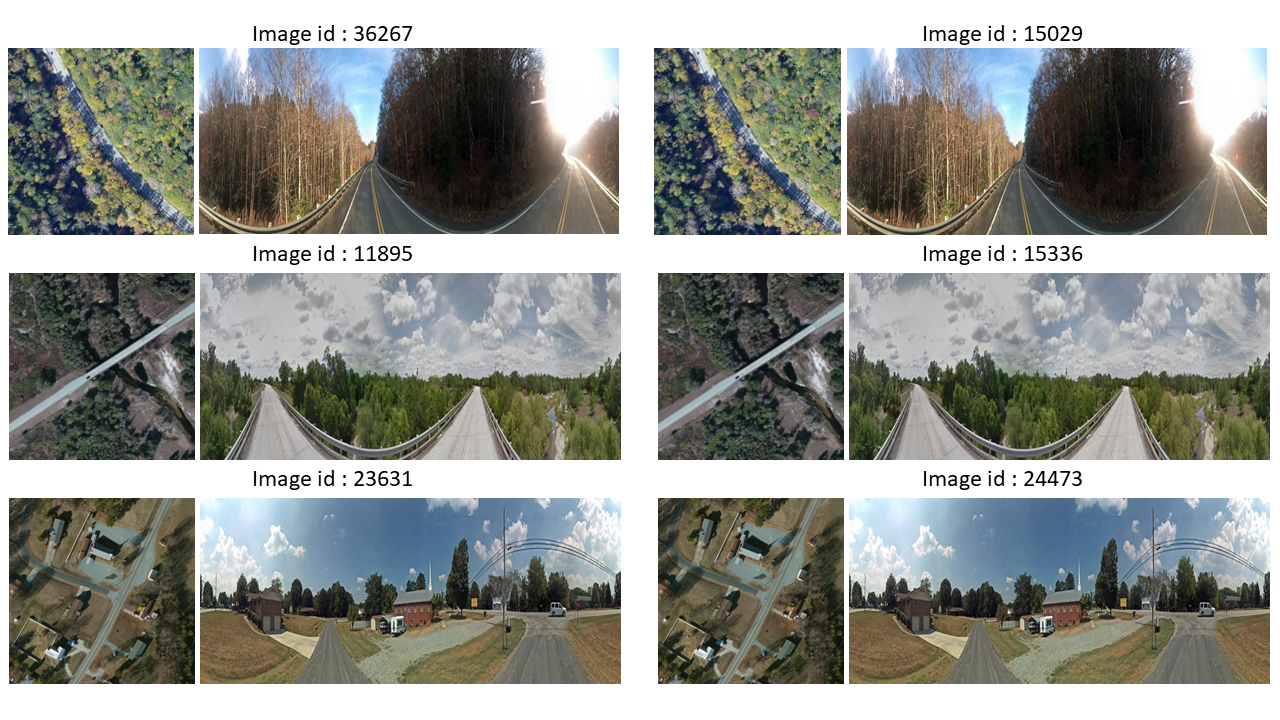
Figure 6: Three examples of repeated ground-aerial pairs from CVUSA training set.

Dataset

To evaluate the effectiveness of GeoDTR+, we conduct extensive experiments on three datasets, CVUSA [2], CVACT [3], and VIGOR [4]. Both CVUSA and CVACT contain $35,532$ training pairs. CVUSA provides $8,884$ pairs for testing and CVACT has the same number of pairs in its validation set (CVACT_val). Besides, CVACT provides a challenging and large-scale testing set (CVUSA_test) which contains $92,802$ pairs. VIGOR is a recently proposed challenging CVGL dataset. Different from CVUSA and CVACT, VIGOR does not assume the one-to-one match and center alignment in aerial-ground pairs. It collects $90,618$ ground panorama images and $105,124$ from 4 major cities in the U.S.A, including, New York, Chicago, Seattle, and San Francisco. Specifically, VIGOR elaborates two protocols, same-area (training and testing on 4 cities) and cross-area (training on New York and Seattle, testing on San Francisco and Chicago) to evaluate the comprehensive performance of CVGL models in metropolitan areas. We sample six aerial-ground image pairs from these three datasets and visualize them in Figure 5. To be noticed that we identify $762$ and $43$ repeated pairs in the original training set and testing set of the CVUSA [2] dataset, respectively. We apply the md5 hash algorithm on the pixel values of each image to identify these repeated pairs. Three random examples with image IDs are presented in Figure 6. For fair comparisons with other baseline methods in this section, we remove the repeated pairs in the training set but keep those in the testing set.

Evaluation Metric

Similar to existing methods [5, 16, 8, 14, 3, 6], we choose to use recall accuracy at top $K$ (R@$K$) for evaluation purposes. R@$K$ measures the probability of the ground truth aerial image ranking within the first $K$ predictions given a query image. In the following experiments, we evaluate the performance of all methods on R@$1$, R@$5$, R@$10$, and R@$1\%$.

Implementation Detail

We set $\alpha$ and $\beta$ in Equation 7 to $10$ and $5$ respectively. The number of transformer encoder layers in the proposed GLE is set to $2$ and each with $4$ heads. The number of descriptors $K$ in Equation 3 is $8$. The model is trained on a single Nvidia V100 GPU for $200$ epochs with AdamW [38] optimizer and a learning rate of $10^{-4}$. The ground images and aerial images are resized to $122\times 671$ and $256\times 256$, respectively. Similar to previous methods [5, 6, 8, 16, 14], we set the batch size to $32$. Within each batch, the exhaustive mini-batch strategy [15] is utilized for constructing triplet pairs. Considering the recently published CVGL models adopt a more advanced backbone (i.e. L2LTR [8] uses ViT [28] and TransGeo leverages DeiT [39]), we upgrade the backbone from our preliminary version of ResNet-34 [40] to ConvNext-T [41] which is more advanced but has a similar number of trainable parameters. Notice that ConvNext-T is a lightweight model and does not outperform ViT [28] and DeiT [39] on ImageNet [42] benchamrk. We take the output before the last average pooling layer of ConvNext-T as the raw feature $\mathbf{r}^{v}$ in Equation 2, the latent feature $f^{v}$ is a $8\times 384=3072$ dimensional vector, where $8$ is $K$ and $384$ is the number of channels in $r^{v}$. All the experiments are performed under the settings mentioned above unless we specify otherwise.

IV-B Main results

TABLE I: Comparison between our GeoDTR+ and baseline methods on CVUSA, CVACT_val, and CVACT_test benchmarks. Magenta text stands for the best results and cyan text stands for the second best result.

Method	CVUSA				CVACT_val				CVACT_test
	R@$1$	R@$5$	R@$10$	R@$1\%$	R@$1$	R@$5$	R@$10$	R@$1\%$	R@$1$	R@$5$	R@$10$	R@$1\%$
w/ PT
CVFT [17]	61.43%	84.69%	90.49%	99.02%	61.05%	81.33%	86.52%	95.93%	26.12%	45.33%	53.80%	71.69%
SAFA [5]	89.84%	96.93%	98.14%	99.64%	81.03%	92.80%	94.84%	98.17%	55.50%	79.94%	85.08%	94.49%
DSM [6]	91.93%	97.50%	98.54%	99.67%	82.49%	92.44%	93.99%	97.32%	35.63%	60.07%	69.10%	84.75%
CDE [16]	92.56%	97.55%	98.33%	99.57%	83.28%	93.57%	95.42%	98.22%	61.29%	85.13%	89.14%	98.32%
L2LTR [8]	94.05%	98.27%	98.99%	99.67%	84.89%	94.59%	95.96%	98.37%	60.72%	85.85%	89.88%	96.12%
SEH [25]	95.11%	98.45%	99.00%	99.78%	84.75%	93.97%	95.46%	98.11%	-	-	-	-
GeoDTR [1]	95.43%	98.86%	99.34%	99.86%	86.21%	95.44%	96.72%	98.77%	64.52%	88.59%	91.96%	98.74%
GeoDTR+ (ours)	95.40%	98.44%	99.05%	99.75%	87.61%	95.48%	96.52%	98.34%	67.57%	89.84%	92.57%	98.54%
w/o PT
CVM-Net [14]	22.47%	49.98%	63.18%	93.62%	20.15%	45.00%	56.87%	87.57%	5.41%	14.79%	25.63%	54.53%
Liu & Li	40.79%	66.82%	76.36%	96.12%	46.96%	68.28%	75.48%	92.01%	19.21%	35.97%	43.30%	60.69%
SAFA [5]	81.15%	94.23%	96.85%	99.49%	78.28%	91.60%	93.79%	98.15%	-	-	-	-
L2LTR [8]	91.99%	97.68%	98.65%	99.75%	83.14%	93.84%	95.51%	98.40%	58.33%	84.23%	88.60%	95.83%
TransGeo [7]	94.08%	98.36%	99.04%	99.77%	84.95%	94.14%	95.78%	98.37%	-	-	-	-
GeoDTR [1]	93.76%	98.47%	99.22%	99.85%	85.43%	94.81%	96.11%	98.26%	62.96%	87.35%	90.70%	98.61%
GeoDTR+ (ours)	95.05%	98.42%	98.92%	99.77%	87.76%	95.50%	96.50%	98.32%	67.75%	90.15%	92.73%	98.53%

IV-B1 CVUSA and CVACT same-area experiment

The same-area evaluation results of the proposed GeoDTR+ and current State-Of-The-Art (SOTA) methods on CVUSA [2] and CVACT [3] are presented in Table I. The best result is indicated in the magenta text, while the second-best result is indicated in the cyan text. As illustrated in Table I, the proposed GeoDTR+ achieves SOTA accuracy on CVACT benchmarks while using the polar transformation. Specifically, on the CVACT_val, GeoDTR+ improves from $86.21\%$ to $87.61\%$ on R@$1$. On one of the most challenging benchmarks, CVACT_test, the proposed model improves from $64.52\%$ to $67.57\%$ on R@$1$. On the CVUSA benchmark, the accuracy of GeoDTR+ is very close to the SOTA value. Without polar transformation, GeoDTR+ achieves SOTA performance on R@$1$ of all three benchmarks. Notably, on CVACT_val and CVACT_test, the proposed model not only achieves SOTA performance but also outperforms results trained with polar transformation, which is not observable in other methods such as SAFA [5] and L2LTR [8]. This can be attributed to the ability of the proposed novel Geometric Layout Extractor (GLE) to explore global spatial configurations.

TABLE II: Cross-area comparison between the proposed GeoDTR+ and baselines on CVUSA and CVACT benchmarks. Magenta text stands for the best results and cyan text stands for the second best result.

Method/Task	CVUSA $\rightarrow$ CVACT				CVACT $\rightarrow$ CVUSA
	R@$1$	R@$5$	R@$10$	R@$1\%$	R@$1$	R@$5$	R@$10$	R@$1\%$
w/ PT
SAFA [5]	30.40%	52.93%	62.29%	85.82%	21.45%	36.55%	43.79%	69.83%
DSM [6]	33.66%	52.17%	59.74%	79.67%	18.47%	34.46%	42.28%	69.01%
L2LTR [8]	47.55%	70.58%	77.39%	91.39%	33.00%	51.87%	60.63%	84.79%
GeoDTR [1]	53.16%	75.62%	81.90%	93.80%	44.07%	64.66%	72.08%	90.09%
GeoDTR+ (ours)	61.17%	80.22%	85.45%	94.56%	53.89%	74.56%	81.10%	94.93%
w/o PT
TransGeo [7]	37.81%	61.57%	69.86%	89.14%	17.45%	32.49%	40.48%	69.14%
GeoDTR [1]	43.72%	66.99%	74.61%	91.83%	29.85%	49.25%	57.11%	82.47%
GeoDTR+ (ours)	60.16%	79.97%	84.67%	94.48%	52.56%	73.08%	79.82%	94.80%

IV-B2 CVUSA and CVACT cross-area experiment

As we discussed in Section I, the generalization of the CVGL models is an important property. Therefore, we conduct a cross-area experiment as presented in Table II. This experiment includes two tasks, training on CVUSA and then testing on CVACT (CVUSA $\rightarrow$ CVACT) and training on CVACT and then testing on CVUSA (CVACT $\rightarrow$ CVUSA). Firstly, as indicated in Table II, GeoDTR+ achieves SOTA performance on all evaluation metrics, both when trained with polar transformation and without polar transformation. Specifically, on CVUSA $\rightarrow$ CVACT task, GeoDTR+ achieves $61.17\%$ and $60.16\%$ R@$1$ accuracy with or without polar transformation which are a significant improvement over the previous SOTA ($8\%$ and $16\%$ respectively). More importantly, we improve R@$1$ in CVACT $\rightarrow$ CVUSA task from previous SOTA $44.07\%$ to $53.89\%$ and from $29.85\%$ to $52.56\%$ on trained with polar transformation and without polar transformation respectively.

TABLE III: Comparison between the proposed GeoDTR+ and baseline methods on VIGOR benchmark. Magenta text stands for the best results and cyan text stands for the second best result.

	Same-area					Cross-area
Method	R@$1$	R@$5$	R@$10$	R@$1\%$	Hit Rate	R@$1$	R@$5$	R@$10$	R@$1\%$	Hit Rate
SAFA [5]	18.69%	43.64%	55.36%	97.55%	21.90%	2.77%	8.61%	12.94%	62.64%	3.16%
SAFA+Mining [4]	38.02%	62.87%	71.12%	97.63%	41.81%	9.23%	21.12%	28.02%	77.84%	9.92%
VIGOR [4]	41.07%	65.81%	74.05%	98.37%	44.71%	11.00%	23.56%	30.76%	80.22%	11.64%
TransGeo [7]	61.48%	87.54%	91.88%	99.56%	73.09%	18.99%	38.24%	46.91%	88.94%	21.21%
GeoDTR [1]	56.51%	80.37%	86.21%	99.25%	61.76%	30.02%	52.67%	61.45%	94.40%	30.19%
GeoDTR+ (ours)	59.01%	81.77%	87.10%	99.07%	67.41%	36.01%	59.06%	67.22%	94.95%	39.40%

IV-B3 VIGOR experiment

To further investigate the performance of GeoDTR+ under more challenging and realistic settings, we benchmark the proposed model on VIGOR [4] dataset. Different from CVUSA [2] and CVACT [3] datasets which maintain a one-to-one correspondence between aerial image and ground image, each ground query image in VIGOR [4] has two or more corresponding aerial images. This setting makes VIGOR [4] closer to real-world scenarios. And due to the many-to-one correspondence, it is considered one of the most challenging datasets in CVGL. Since the evaluation protocol in VIGOR includes same-area configuration and cross-area configuration. So we did not conduct separate cross-area experiments on other datasets. Table III presents the performance comparison between the proposed GeoDTR+ and other baseline methods. GeoDTR+ achieves the SOTA performance by improving from the previous SOTA $18.99\%$ to $36.01\%$ which is a $17.02\%$ increasing in cross-area experiment. Although, GeoDTR+ does not achieve the best result on same-area evaluation. But the performance gap is relatively small considering the improvement in the cross-area experiment. In summary, GeoDTR+ shows comparable performance with the existing SOTA on same-area evaluation and significantly enhances the cross-area performance on cross-area evaluation. In the next section, we conduct ablation studies to demonstrate the effectiveness of the number of descriptors, the proposed GLE, and CHSG on our model.

IV-C Ablation studies

TABLE IV: Ablation study of the proposed Geometric Layout Extractor (GLE) and CHSG on CVUSA and CVACT dataset with same-area and cross-area evaluation. In the GLE configuration, “v1” stands for the GLE from our preliminary work [1]. “v2” stands for the GLE proposed in this work.

	Configurations			Same-area				Cross-area
	CHSG	GLE	Backbone	R@$1$	R@$5$	R@$10$	R@$1\%$	R@$1$	R@$5$	R@$10$	R@$1\%$
CVUSA	$\times$	v1	ResNet-34	95.43%	98.86%	99.34%	99.86%	53.16%	75.62%	81.90%	93.80%
	$\checkmark$	v1	ResNet-34	94.97%	98.47%	98.98%	99.73%	57.03%	76.92%	82.77%	93.87%
	$\times$	v2	ResNet-34	94.88%	98.37%	98.99%	99.76%	54.05%	75.93%	82.58%	93.94%
	$\checkmark$	v2	ResNet-34	94.26%	98.21%	98.91%	99.71%	59.72%	78.78%	82.95%	92.37%
	$\times$	v2	ConvNeXt-T	95.77%	98.93%	99.36%	99.81%	53.65%	74.91%	81.39%	93.27%
	$\checkmark$	v2	ConvNeXt-T	95.40%	98.44%	99.05%	99.75%	61.17%	80.22%	85.45%	94.56%
CVACT	$\times$	v1	ResNet-34	86.21%	95.44%	96.72%	98.77%	44.07%	64.66%	72.08%	90.09%
	$\checkmark$	v1	ResNet-34	86.48%	95.26%	96.58%	98.26%	50.63%	71.26%	78.50%	93.87%
	$\times$	v2	ResNet-34	85.86%	95.06%	96.30%	98.38%	45.44%	66.07%	72.35%	90.97%
	$\checkmark$	v2	ResNet-34	86.19%	94.90%	96.29%	98.30%	49.09%	70.65%	79.09%	93.42%
	$\times$	v2	ConvNeXt-T	88.18%	95.57%	96.68%	98.67%	42.11%	62.00%	70.58%	90.88%
	$\checkmark$	v2	ConvNeXt-T	87.61%	95.48%	96.52%	98.34%	53.89%	74.56%	81.10%	94.93%

IV-C1 Ablation study of GLE, CHSG, and Backbone

To investigate the attribute of each component in the GeoDTR+, we conduct an ablation study of the proposed GLE (Section III-C2) and CHSG (Section III-E). The results are presented in Table IV. All experiments in Table IV are trained with LS techniques by default. We vary the combination of the GLE, CHSG, and backbones. As shown in Table IV, we first can observe the difference by comparing the proposed GLE in this work (“v2”) and GLE from our preliminary work [1] (“v1”). As we can see that training with the novel GLE (v2) on ResNet-34 [40] improves the cross-area performance on both CVUSA and CVACT datasets. For example, the R@$1$ accuracy improves from $44.07\%$ (line 1) to $45.44\%$ (line 3) on the CVACT dataset. On the other hand, CHSG also plays a vital role in boosting performance. By comparing each pair of experiments training with and without CHSG, we observe that CHSG significantly enhances the performance on cross-area benchmarks while having minimal impact on the same-area performance. For instance, while training on ConvNeXt-T with the proposed GLE, training without CHSG only achieves $42.11\%$ on the CVACT dataset. However, when training with CHSG, this number increases to $53.89\%$. Lastly, we find that upgrading the backbone slightly improves the same-area performance. However, the cross-area performance degrades if training without CHSG (i.e. line 3 and line 5 in both CVUSA and CVACT experiment from Table IV). Once training with CHSG, this degradation can be mitigated due to the strong supervision signal from the additional hard aerial-ground pairs. To reveal the underlying mechanism of the proposed GLE and CHSG, We provide more complete investigations as well as more detailed experiments and analyses in Section V.

TABLE V: Ablation study of different numbers of descriptors (2,4,6,8) and their corresponding latent feature dimensions on CVUSA and CVACT datasets.

			Same-area				Cross-area
	# of Des.	Dimension	R@$1$	R@$5$	R@$10$	R@$1\%$	R@$1$	R@$5$	R@$10$	R@$1\%$
CVUSA	8	3072	95.40%	98.44%	99.05%	99.75%	61.17%	80.22%	85.45%	94.56%
	6	2304	95.09%	98.38%	99.04%	99.73%	60.73%	79.68%	84.97%	95.21%
	4	1536	94.57%	98.32%	98.96%	99.67%	60.21%	79.43%	85.86%	94.27%
	2	768	93.59%	98.08%	98.87%	99.65%	59.21%	78.96%	84.48%	94.06%
CVACT	8	3072	87.61%	95.48%	96.52%	98.34%	53.89%	74.56%	81.10%	94.93%
	6	2304	87.05%	95.33%	96.55%	98.41%	53.61%	73.97%	80.69%	94.57%
	4	1536	86.85%	95.42%	96.62%	98.26%	52.75%	73.30%	80.36%	94.51%
	2	768	86.22%	94.96%	96.37%	98.22%	50.68%	71.12%	78.89%	94.10%

IV-C2 Effect of GLE descriptors

CVGL is sensitive to the latent feature dimensions in a real-world deployment. Smaller latent feature dimensions shorten the inference time and require less reference feature storage space. In our proposed GeoDTR+, we can change the latent dimensions by varying the number of GLDs. The result is illustrated in Table V. It is clear to see that with the smaller latent feature dimensions, both the same-area and cross-area performance degrade. However, to be noticed, even with $2$ descriptors and $768$ latent dimensions, our model still achieves SOTA performance on cross-area benchmarks. More importantly, the degradation of the same-area result does not exceed $2\%$ which means the model is still comparable to the existing SOTA result on same-area benchmarks.

TABLE VI: Comparison of the proposed GeoDTR+ trained with different data sampling strategies with different batch sizes on the CVUSA dataset. “RAW” stands for the original aerial-ground pairs as input without any augmentation. “BS” is short for batch size. The model is trained on the CVUSA dataset and evaluated on both same-area and cross-area benchmarks.

	Configuration	BS	R@$1$	R@$5$	R@$10$	R@$1\%$
Same-area	Raw	32	95.77%	98.93%	99.36%	99.81%
	LS	32	95.90%	98.96%	99.42%	99.81%
	LS	64	96.24%	99.04%	99.51%	99.84%
	CHSG	32	95.40%	98.44%	99.05%	99.75%
Cross-area	Raw	32	53.65%	74.91%	81.39%	93.27%
	LS	32	58.62%	78.53%	84.20%	94.09%
	LS	64	57.18%	78.33%	84.14%	93.72%
	CHSG	32	61.17%	80.22%	85.45%	94.56%

IV-C3 Effect of CHSG over LS

To better evaluate the effect of CHSG on the CVGL performance, in addition to the plain LS, we conduct experiments with LS, CHSG, and various batch sizes, as shown in Table VI. We first note that different configurations share similar same-area performance. However, without LS techniques and CHSG, the model performs poorly on cross-area benchmarks. We also observe that a larger batch size ($64$) with LS techniques can have a marginal performance improvement in the same-area evaluation compared with the standard batch size ($32$) with LS techniques. Still, the cross-area performance remains at a similar level compared with the standard batch size. More importantly, compared with other configurations, training with CHSG can significantly boost the cross-area performance, achieving $61.17\%$ on R@$1$, while maintaining a batch size of $32$. This demonstrates that simply increasing the batch size can hardly improve both same-area and cross-area performance. But CHSG can efficiently guide the model to learn more distinct geometric patterns which is helpful in improving cross-area performance. Section V includes additional fine-grained experiments to further demonstrate the contributions in CHSG at inter- and intra-batch levels.

TABLE VII: Computational efficiency comparison between the proposed GeoDTR+ and GeoDTR [1], TransGeo [7], L2LTR [8]. All experiments are conducted on a single Nvidia V100 GPU.

Method	# of Parameters	Inference Time	Pretraining model	Computational Cost
L2LTR [8]	195.9M	405ms	ImageNet-21K for ViT	46.77 GFLOPS
TransGeo [7]	44.0M	99ms	ImageNet-1K for DeiT	11.35 GFLOPS
GeoDTR [1]	48.5M	235ms	ImageNet-1K for ResNet34	39.89 GFLOPS
GeoDTR+ (ours)	24.7M	103ms	ImageNet-1K for ConvNeXt-Tiny	11.25 GFLOPS

IV-D Computational Efficiency

To better understand the proposed GeoDTR+ in inference efficiency, we compare the number (#) of the trainable parameters, inference time, pretrained model, and computational cost for GeoDTR+ and recently published methods as presented in Table VII. It is clear to see that GeoDTR+ has the least # of trainable parameters because of the new GLE design and the ConvNeXt-T [41] backbone. Compared with GeoDTR [1] and TransGeo [7], GeoDTR+ has $50\%$ and $45\%$ less trainable parameters respectively. Our model has similar inference time and floating point operations per second to TransGeo [7] which is one of the lightest models in CVGL. Compared with L2LTR [8], GeoDTR+ does not require a large pretrained backbone such as ViT which is pretrained on ImageNet-21K [42].

Figure 7: Visualization of the learned descriptors from the proposed GeoDTR+ training with polar transformation (a) and without polar transformation (b). The images at the top are the input ground images and aerial images accordingly. From top to bottom are the first to the eighth heatmap visualization of learned descriptors. For better visualization purposes, we apply the polar transformation on the aerial descriptors from the model training without polar transformation(b). We note a strong alignment of the learned descriptors in both (a) and (b) which demonstrates the ability of GeoDTR+ to capture the geometric correspondence. This also illustrates the reason that our model shows a similar performance while training with or without polar transformation.

Figure 8: Comparison between the first two learned descriptors between the preliminary GeoDTR and the proposed GeoDTR+. (a) and (c) are descriptors from the proposed GeoDTR+ trained with or without polar transformation respectively. (b) and (c) are descriptors from the preliminary GeoDTR trained with or without polar transformation respectively. In each sub-figure, the left is the ground image descriptor and the aerial image descriptor is on the right-hand side. Noticed that despite the polar transformation, GeoDTR+ learns more concentrated regions than GeoDTR which implies that GeoDTR+ learns a more distinguishable latent representation.

V Discussion

V-A Discussion of Geometric Layout Descriptors

Same-area performance has always been the main focus of Cross-View Geo-Localization (CVGL) methods for a long time. While the increase in same-area performance gradually reaches its margin, there is still a huge performance gap between cross-area and same-area cases. In this work, we propose to highlight the cross-area performance as it reflects the actual utility of a CVGL model in real-world scenarios as discussed in Section I. Furthermore, the failure of generalizing to unseen areas might indicate overfitting of the model under consideration.

One possible way to address the cross-area generalization is to exploit the correspondence between the layouts of visual features in the ground and aerial images. The geometric constraints underlying this correspondence are the same despite the dramatic change in the appearance of visual features from different areas. Following this philosophy, we introduce a specialized pathway in GeoDTR+ for capturing the geometric layout of visual features.

Concretely, we model the geometric layout through a set of mask-like descriptors $\mathbf{q}$, which at output modulate the raw backbone feature (see Equation 2). Elements in a descriptor take value from the range $[0,1]$ and each descriptor only deviates from zero at scattered areas that distribute across the whole spatial range. Consequently, a descriptor filters out distinct “active” areas from the backbone feature for the final comparison. The essential characteristics of Geometric Layout Descriptors (GLD) can be expressed as follows,

• Capturing the correlations among visual features, i.e., visual features within the active areas are considered to be correlated;

• Presenting the global property, i.e., the active areas distribute across the whole spatial range.

Our descriptor-based representation of geometric layout shares other benefits. First, during the forward pass, the descriptors help pick up discriminative components from the raw backbone feature, leading to more efficient use of information in the backbone feature. Second, only elements within the active areas receive significant gradients signal during back-propagation. This makes the training easier as it needs not to tune the full backbone feature.

To justify the above picture and fully demonstrate the power of our model, we visualize the ground and aerial descriptors in Figure 7 for cases when GeoDTR+ is trained with polar transformed aerial images and normal aerial images (without polar transformation), respectively. As shown in the Figure 7(a), we first note a strong alignment between descriptors of a given aerial-ground pair. It is clear to see that the corresponding descriptors share very similar salient values. More strikingly, such an alignment still exists when our model is trained with normal ground images. In Figure 7(b), we unroll the descriptors for the normal aerial image by polar transformation. We observe that apart from the deformation brought by the polar transformation, the locations of salient patterns in the aerial descriptors match those in the corresponding ground descriptors. This indicates the ability of GeoDTR+ to grasp the geometric correspondence even without the guidance of polar transformation and it also demonstrates the reason why the performance of GeoDTR+ training with or without polar transformation is extremely close and both achieve outstanding performance. Moreover, we compare the first two descriptors from the preliminary GeoDTR and the proposed GeoDTR+ trained with polar transformation and without it in Figure 8. It is clear to see that despite the polar transformation, GeoDTR+ learns more concentrated regions than GeoDTR which implies that GeoDTR+ learns a more distinguishable latent representation.

V-B Discussion of Contrastive Hard Samples Generation

Besides the geometric layout, we further integrate the proposed novel sampling strategy named Contrastive Hard Samples Generation (CHSG), which produces hard samples that share similar patterns while differing in layout in a single training batch. This introduced intra-batch contrast over hard samples enables the GeoDTR+ to efficiently learn discriminative features. Ultimately, CHSG can push the model away from the local minimum and achieve better cross-area performance. Moreover, different from existing hard mining strategies in CVGL [31, 4], CHSG does not rely on a mining pool to maintain the global similarities among all the training samples. Thus, CHSG is more efficient in terms of both training time and memory usage.

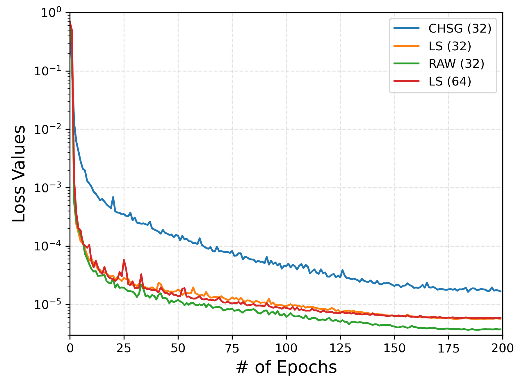
Figure 9: Comparison of triplet loss values of GeoDTR+ during training with different configurations on CVUSA dataset. “CHSG” stands for training with CHSG. “LS” stands for training with LS techniques. “RAW” stands for training without LS and CHSG. The number in the brackets is the batch size.

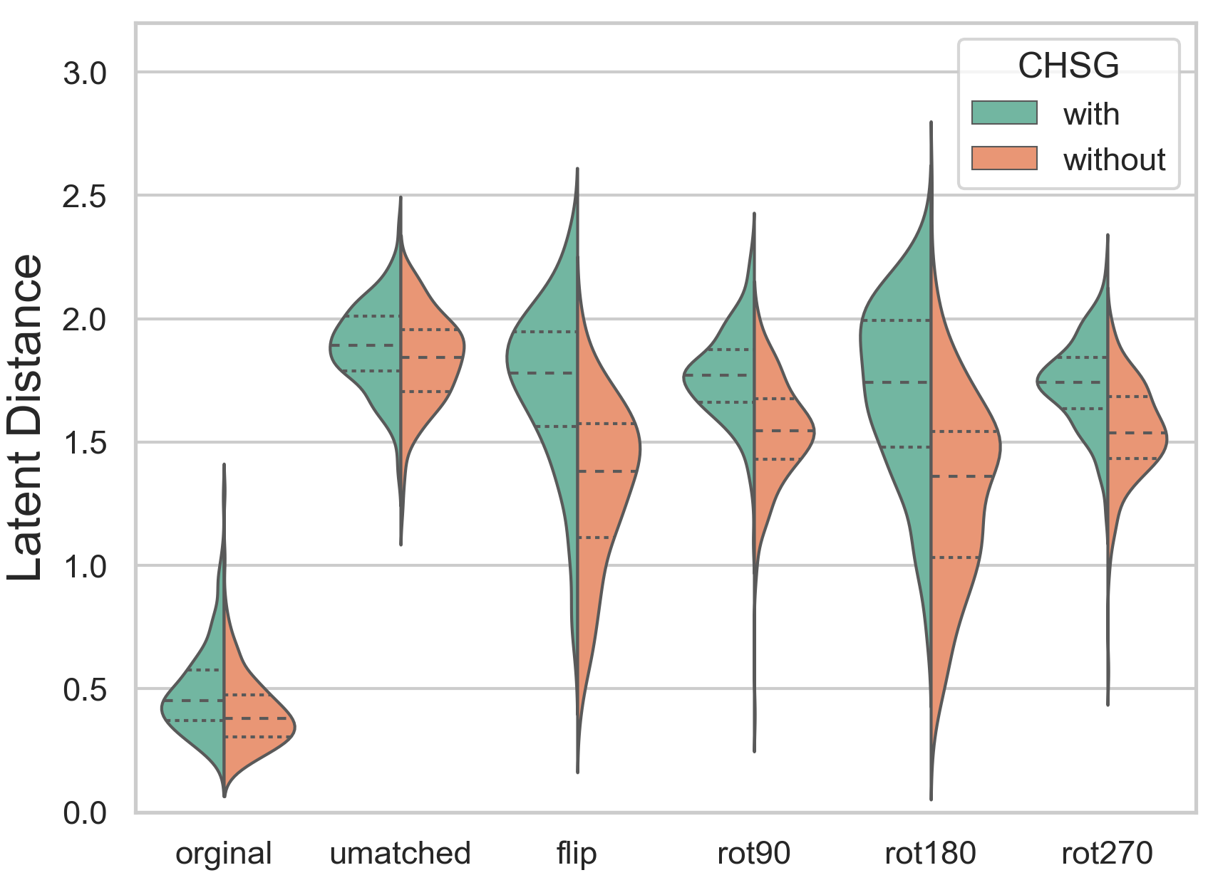
Figure 10: Latent feature distance violin plot of GeoDTR+ training with CHSG and training without CHSG on $200$ random test aerial-ground pairs. From left to right on the x-axis, “original” stands for original aerial-ground pairs, and “unmatched” stands for random unmatched aerial-ground pairs. “flip”, “rot90”, “rot180”, “rot270” are fixing the aerial image, and flipping or rotating the ground images horizontally or in certain degrees respectively.

TABLE VIII: Comparison of GeoDTR+ trained with different configurations of the proposed CHSG on CVUSA dataset. “RAW” refers to training with original aerial-ground pairs. “S” is short for semantic augmentation. “L” is short for Layout simulation. “same” means the same operation (L or S) is applied to both contrastive samples $P_{L_{\gamma}}$ and $P_{L_{\delta}}$.

	Configuration	R@$1$	R@$5$	R@$10$	R@$1\%$
Same-area	Raw	95.77%	98.93%	99.36%	99.81%
	S only	94.78%	98.53%	99.12%	99.70%
	S + same L	95.62%	99.00%	99.40%	99.84%
	L only	95.52%	98.57%	99.14%	99.76%
	same S + L	95.55%	98.64%	99.12%	99.75%
	L + S	95.40%	98.44%	99.05%	99.75%
Cross-area	Raw	53.65%	74.91%	81.39%	93.27%
	S only	55.77%	77.04%	82.28%	93.46%
	S + same L	59.16%	79.72%	85.06%	94.55%
	L only	58.09%	78.08%	84.18%	93.73%
	same S + L	59.46%	79.82%	85.61%	94.46%
	L + S	61.17%	80.22%	85.45%	94.56%

Results in Tables VIII and VI confirm the benefits of CHSG on our model, especially the improvement in cross-area performance. In order to understand how the CHSG improves the model, we first visualize the loss values during training under different configurations in Figure 9. In the plot, the experiment trained with vanilla triplet loss serves the baseline and is compared with the ones trained with LS and CHSG. To demonstrate the effects of intra-batch contrast, two configurations of training with LS are included, one with a batch size of $32$ and the other of $64$. While all models converge at a similar rate, applying CHSG leads to a significantly and consistently higher loss than the other three configurations, thus providing a stronger supervision signal for the training. The losses of training with LS are constantly higher than the one training without it but have a noticeable gap to the loss of training with CHSG. It is interesting to note that the loss curve of LS ($64$) is almost identical to that of LS ($32$). Recall that CHSG generates two variations from each original pair. In this sense, it doubles the batch size, and therefore the difference between CHSG ($32$) and LS ($64$) indicates that the increase in loss is a result of introducing hard contrastive samples.

Next, we seek to investigate the different behaviors of the model trained with CHSG and with LS alone. Specifically, we care about the latent feature distance between a ground image and an aerial image. This experiment is carried out with $200$ randomly sampled test data from the CVUSA dataset, and Figure 10 shows the distribution of latent feature distance for different types of aerial-ground pairs. In the plot, “original” refers to the ground truth aerial-ground pairs. “unmatched” stands for randomly constructed unmatched aerial-ground pairs. “flip”, “rot90”, “rot180” and “rot270” refers to those hard samples with respect to the ground truth aerial-ground pairs. They are constructed by fixing the aerial image and flipping or rotating the ground truth ground image at certain degrees respectively. As expected, the “original” case has the lowest mean latent feature distance while the “unmatched” shows the largest. Noticeably the distributions are similar for models trained with and without CHSG. However, those hard samples show different distributions of latent feature distance from the two models. While training without the proposed CHSG, the distance distributions of hard samples favor smaller values and, hence, the model cannot distinguish them well from the ground truth pairs. On the other hand, when trained with CHSG the distance distributions of hard samples all shift towards larger values and become comparable with the ones of unmatched aerial-ground pairs. This makes sense since flipping and rotation break the geometric correspondence in aerial-ground pairs. So that they can be considered as effective “unmatched” pairs. The ability to better distinguish hard samples endorses the outstanding performance of our model.

The previous discussion emphasizes the importance of the intra-batch contrast among hard samples. It is interesting to have a fine-grained analysis of CHSG on how the semantic augmentation and layout simulation components contribute at the inter-batch and the intra-batch levels. Thus, we compare four different settings of CHSG where the hard samples are generated by applying

• different layout simulations only (L only)

• different semantic augmentations only (S only)

• same layout simulation and different semantic augmentations (same L $+$ S)

• same semantic augmentation and different layout simulations (same S $+$ L)

In the same L + S case, the effects of layout simulation happen at the inter-batch level while the effects of semantic augmentation at the intra-batch level (similar to the L + same S case).

Table VIII summarizes the results. We found that inter-batch contrast with either semantic augmentation or layout simulation can boost the model on cross-area performance (L only or S only). Adding additional intra-batch contrastive signals (same L $+$ S or same S $+$ L) can further improve the accuracy. Best performance is achieved when both contrastive signals operate at the intra-batch level (L + S). Moreover, we found that adding either inter-batch or intra-batch contrast can hardly be harmful to the model on same-area performance. In other words, the results with adding contrast remain at the same level of performance as the one without adding any contrast (“Raw” in Table VIII). The above results confirm the contribution of the intra-batch contrast on the cross-area performance while not hurting the same-area results.

VI conclusion

In conclusion, we extend our preliminary work GeoDTR [1] to address the problem of loss of information in geometric layout descriptor extraction and further explore the usage of LS techniques in improving cross-area cross-view geo-localization. In this paper, we propose GeoDTR+ to explicitly disentangles the geometric layout correlations from the raw features extracted by the backbone feature extractor via a novel Geometric Layout Extractor (GLE). The latent representation is a Frobenius product between the raw features and geometric layout extractors which effectively captures geometric correspondence between aerial and ground images, even without post-processing such as polar transformation. To push the limit of cross-area cross-view geo-localization, we take advantage of LS techniques and form a Contrastive Hard Sample Generation (CHSG) sampling strategy. CHSG aims to generate hard aerial-ground image pairs by varying the geometric layout and low-level details. Thus, there is no need to mine hard samples from a global pool which cost extra computational resources. Our experiment demonstrated that the proposed GeoDTR+ achieves state-of-the-art (SOTA) results on CVACT_val [3] which is one of the most challenging same-area benchmarks. Meanwhile, GeoDTR+ maintains a comparable same-area performance with other SOTA methods on CVUSA [2] and VIGOR [4]. Most importantly, the proposed GeoDTR+ achieves SOTA performance on all cross-area benchmarks including, CVUSA [2], CVACT [3], and VIGOR [4] with a considerable improvement from the existing methods.

For future research, considering the ability of generalization of the proposed GeoDTR+, it is worth investigating the performance of GeoDTR+ under different environments, for example, low-light scenarios or different seasons. It is also worth extending the usage of CHSG under other contrastive learning or image retrieval tasks to see how it works.

VII Biography Section

Xiaohan Zhang is a third-year Ph.D. student at the University of Vermont advised by Dr.Safwan Wshah. His current research interest lies at the border of computer vision and remote sensing (e.g. visual geo-localization and segmentation/detection in aerial images). He is also interested in image synthesis and 3D reconstruction. Before joining the University of Vermont, he received his M.Sc. degree at the University of California, Santa Cruz in 2020, and he obtained his B.Sc. degree at Michigan State University in 2017.

Dr. Xingyu Li is currently an Assistant Researcher at Lin Gang Laboratory, Shanghai. He received his M.Sc. degree in computer science from the University of California, Santa Cruz in 2020, and his Ph.D. degree in atomic and molecular physics from the University of Science and Technology of China, Hefei in 2017. He was a post-doctoral researcher with Shanghai Center for Brain Science and Brain-Inspired Technology during 2021.07-2023.07. His research interests include deep learning, cognitive neuroscience, and brain-inspired intelligence.

Dr. Waqas Sultani is an Assistant Professor at the Information Technology University, Lahore. He received his Ph.D. from the Center for Research in Computer Vision at UCF. His research related to human action recognition, anomaly detection, small object detection, geolocalization, and medical imaging got published in the top venues including CVPR, ICRA, AAAI, WACV, CVIU, MICCAI, etc. He was awarded the Facebook-CV4GC research award in 2019 and a Google Research Scholar award in 2023 for projects related to medical imaging. He also served as an area chair for several conferences such as CVPR 2022-2024, and ACM-MM 2020-2021.

Dr. Chen Chen is an Assistant Professor at the Center for Research in Computer Vision at UCF. He received his Ph.D. in Electrical Engineering from UT Dallas in 2016, receiving the David Daniel Fellowship (Best Doctoral Dissertation Award). His research interests include computer vision, efficient deep learning, and federated learning. He has been actively involved in several NSF and industry-sponsored research projects, focusing on efficient resource-aware machine vision algorithms and systems development for large-scale camera networks. He is an Associate Editor of IEEE Transactions on Circuits and Systems for Video Technology (T-CSVT), Journal of Real-Time Image Processing, and IEEE Journal on Miniaturization for Air and Space Systems. He also served as an area chair for several conferences such as ECCV’2022, CVPR’2022, ACM-MM 2019-2022, ICME 2021 and 2022. According to Google Scholar, he has 13K+ citations and an h-index of 55.

Dr. Safwan Wshah is currently an Assistant Professor in the Department of Computer Science at the University of Vermont. His research interests lie at the intersection of machine learning theory and application. His core area is object understanding and geo-localization from the ground, aerial and satellite images.He also has broader interests in deep learning, computer vision, data analytics, and image processing. Dr. Wshah received his Ph.D. in Computer Science and Engineering from the University at Buffalo in 2012. Prior to joining the University of Vermont, Dr. Wshah worked for Xerox and PARC (Palo Alto Research Center)- Xerox company, where he was involved in several projects creating machine learning algorithms for different applications in healthcare, transportation, and education fields.

References

- [1] X. Zhang, X. Li, W. Sultani, Y. Zhou, and S. Wshah, “Cross-view geo-localization via learning disentangled geometric layout correspondence,” arXiv preprint arXiv:2212.04074, 2022.
- [2] S. Workman, R. Souvenir, and N. Jacobs, “Wide-area image geolocalization with aerial reference imagery,” in Proceedings of the IEEE International Conference on Computer Vision (ICCV), December 2015.
- [3] L. Liu and H. Li, “Lending orientation to neural networks for cross-view geo-localization,” in Proceedings of the IEEE/CVF Conference on Computer Vision and Pattern Recognition (CVPR), June 2019.
- [4] S. Zhu, T. Yang, and C. Chen, “Vigor: Cross-view image geo-localization beyond one-to-one retrieval,” in Proceedings of the IEEE/CVF Conference on Computer Vision and Pattern Recognition (CVPR), June 2021, pp. 3640–3649.
- [5] Y. Shi, L. Liu, X. Yu, and H. Li, “Spatial-aware feature aggregation for image based cross-view geo-localization,” Advances in Neural Information Processing Systems, vol. 32, pp. 10 090–10 100, 2019.
- [6] Y. Shi, X. Yu, D. Campbell, and H. Li, “Where am i looking at? joint location and orientation estimation by cross-view matching,” in Proceedings of the IEEE/CVF Conference on Computer Vision and Pattern Recognition (CVPR), June 2020.
- [7] S. Zhu, M. Shah, and C. Chen, “Transgeo: Transformer is all you need for cross-view image geo-localization,” in Proceedings of the IEEE/CVF Conference on Computer Vision and Pattern Recognition (CVPR), June 2022, pp. 1162–1171.
- [8] H. Yang, X. Lu, and Y. Zhu, “Cross-view geo-localization with layer-to-layer transformer,” in Advances in Neural Information Processing Systems, M. Ranzato, A. Beygelzimer, Y. Dauphin, P. Liang, and J. W. Vaughan, Eds., vol. 34. Curran Associates, Inc., 2021, pp. 29 009–29 020.
- [9] D. Wilson, X. Zhang, W. Sultani, and S. Wshah, “Visual and object geo-localization: A comprehensive survey,” arXiv preprint arXiv:2112.15202, 2021.
- [10] D.-K. Kim and M. R. Walter, “Satellite image-based localization via learned embeddings,” in 2017 IEEE International Conference on Robotics and Automation (ICRA), 2017, pp. 2073–2080.
- [11] A. Shetty and G. X. Gao, “Uav pose estimation using cross-view geolocalization with satellite imagery,” in 2019 International Conference on Robotics and Automation (ICRA), 2019, pp. 1827–1833.
- [12] D. Wilson, T. Alshaabi, C. Van Oort, X. Zhang, J. Nelson, and S. Wshah, “Object tracking and geo-localization from street images,” Remote Sensing, vol. 14, no. 11, 2022. [Online]. Available: https://www.mdpi.com/2072-4292/14/11/2575
- [13] H.-P. Chiu, V. Murali, R. Villamil, G. D. Kessler, S. Samarasekera, and R. Kumar, “Augmented reality driving using semantic geo-registration,” in 2018 IEEE Conference on Virtual Reality and 3D User Interfaces (VR), 2018, pp. 423–430.
- [14] S. Hu, M. Feng, R. M. Nguyen, and G. H. Lee, “Cvm-net: Cross-view matching network for image-based ground-to-aerial geo-localization,” in Proceedings of the IEEE Conference on Computer Vision and Pattern Recognition, 2018, pp. 7258–7267.
- [15] N. N. Vo and J. Hays, “Localizing and orienting street views using overhead imagery,” in Computer Vision – ECCV 2016, B. Leibe, J. Matas, N. Sebe, and M. Welling, Eds. Cham: Springer International Publishing, 2016, pp. 494–509.
- [16] A. Toker, Q. Zhou, M. Maximov, and L. Leal-Taixe, “Coming down to earth: Satellite-to-street view synthesis for geo-localization,” in Proceedings of the IEEE/CVF Conference on Computer Vision and Pattern Recognition (CVPR), June 2021, pp. 6488–6497.
- [17] Y. Shi, X. Yu, L. Liu, T. Zhang, and H. Li, “Optimal feature transport for cross-view image geo-localization,” Proceedings of the AAAI Conference on Artificial Intelligence, vol. 34, no. 07, pp. 11 990–11 997, Apr. 2020.
- [18] T. Wang, Z. Zheng, C. Yan, J. Zhang, Y. Sun, B. Zheng, and Y. Yang, “Each part matters: Local patterns facilitate cross-view geo-localization,” IEEE Transactions on Circuits and Systems for Video Technology, pp. 1–1, 2021.
- [19] Z. Zheng, Y. Wei, and Y. Yang, “University-1652: A multi-view multi-source benchmark for drone-based geo-localization,” in Proceedings of the 28th ACM International Conference on Multimedia, ser. MM ’20. New York, NY, USA: Association for Computing Machinery, 2020, p. 1395–1403.
- [20] T.-Y. Lin, Y. Cui, S. Belongie, and J. Hays, “Learning deep representations for ground-to-aerial geolocalization,” in Proceedings of the IEEE Conference on Computer Vision and Pattern Recognition (CVPR), June 2015.
- [21] S. Cai, Y. Guo, S. Khan, J. Hu, and G. Wen, “Ground-to-aerial image geo-localization with a hard exemplar reweighting triplet loss,” in Proceedings of the IEEE/CVF International Conference on Computer Vision (ICCV), October 2019.
- [22] A. Vaswani, N. Shazeer, N. Parmar, J. Uszkoreit, L. Jones, A. N. Gomez, L. u. Kaiser, and I. Polosukhin, “Attention is all you need,” in Advances in Neural Information Processing Systems, I. Guyon, U. V. Luxburg, S. Bengio, H. Wallach, R. Fergus, S. Vishwanathan, and R. Garnett, Eds., vol. 30. Curran Associates, Inc., 2017.
- [23] X. Zhang, W. Sultani, and S. Wshah, “Cross-view image sequence geo-localization,” in Proceedings of the IEEE/CVF Winter Conference on Applications of Computer Vision (WACV), January 2023, pp. 2914–2923.
- [24] T.-Y. Lin, S. Belongie, and J. Hays, “Cross-view image geolocalization,” in Proceedings of the IEEE Conference on Computer Vision and Pattern Recognition (CVPR), June 2013.
- [25] Y. Guo, M. Choi, K. Li, F. Boussaid, and M. Bennamoun, “Soft exemplar highlighting for cross-view image-based geo-localization,” IEEE transactions on image processing, vol. 31, pp. 2094–2105, 2022.
- [26] K. Regmi and M. Shah, “Bridging the domain gap for ground-to-aerial image matching,” in Proceedings of the IEEE/CVF International Conference on Computer Vision (ICCV), October 2019.
- [27] I. Goodfellow, J. Pouget-Abadie, M. Mirza, B. Xu, D. Warde-Farley, S. Ozair, A. Courville, and Y. Bengio, “Generative adversarial nets,” Advances in neural information processing systems, vol. 27, 2014.
- [28] A. Dosovitskiy, L. Beyer, A. Kolesnikov, D. Weissenborn, X. Zhai, T. Unterthiner, M. Dehghani, M. Minderer, G. Heigold, S. Gelly, J. Uszkoreit, and N. Houlsby, “An image is worth 16x16 words: Transformers for image recognition at scale,” in International Conference on Learning Representations, 2021.
- [29] R. Rodrigues and M. Tani, “Global assists local: Effective aerial representations for field of view constrained image geo-localization,” in Proceedings of the IEEE/CVF Winter Conference on Applications of Computer Vision (WACV), January 2022, pp. 3871–3879.
- [30] ——, “Are these from the same place? seeing the unseen in cross-view image geo-localization,” in Proceedings of the IEEE/CVF Winter Conference on Applications of Computer Vision (WACV), January 2021, pp. 3753–3761.
- [31] S. Zhu, T. Yang, and C. Chen, “Revisiting street-to-aerial view image geo-localization and orientation estimation,” in Proceedings of the IEEE/CVF Winter Conference on Applications of Computer Vision (WACV), January 2021, pp. 756–765.
- [32] J. Pearl, Causality: Models, Reasoning and Inference, 2nd ed. USA: Cambridge University Press, 2009.
- [33] R. M. Byrne, “Counterfactuals in explainable artificial intelligence (xai): Evidence from human reasoning.” in IJCAI, 2019, pp. 6276–6282.
- [34] E. Abbasnejad, D. Teney, A. Parvaneh, J. Shi, and A. v. d. Hengel, “Counterfactual vision and language learning,” in Proceedings of the IEEE/CVF Conference on Computer Vision and Pattern Recognition (CVPR), June 2020.
- [35] F. Baradel, N. Neverova, J. Mille, G. Mori, and C. Wolf, “Cophy: Counterfactual learning of physical dynamics,” in International Conference on Learning Representations, 2020.
- [36] Y. Wang, Y. Wan, C. Zhang, L. Bai, L. Cui, and P. Yu, “Competitive multi-agent deep reinforcement learning with counterfactual thinking,” in 2019 IEEE International Conference on Data Mining (ICDM). IEEE, 2019, pp. 1366–1371.
- [37] Y. Rao, G. Chen, J. Lu, and J. Zhou, “Counterfactual attention learning for fine-grained visual categorization and re-identification,” in Proceedings of the IEEE/CVF International Conference on Computer Vision (ICCV), October 2021, pp. 1025–1034.
- [38] I. Loshchilov and F. Hutter, “Decoupled weight decay regularization,” arXiv preprint arXiv:1711.05101, 2017.
- [39] H. Touvron, M. Cord, M. Douze, F. Massa, A. Sablayrolles, and H. Jégou, “Training data-efficient image transformers & distillation through attention,” in International conference on machine learning. PMLR, 2021, pp. 10 347–10 357.
- [40] K. He, X. Zhang, S. Ren, and J. Sun, “Deep residual learning for image recognition,” in Proceedings of the IEEE Conference on Computer Vision and Pattern Recognition (CVPR), June 2016.
- [41] Z. Liu, H. Mao, C.-Y. Wu, C. Feichtenhofer, T. Darrell, and S. Xie, “A convnet for the 2020s,” in Proceedings of the IEEE/CVF Conference on Computer Vision and Pattern Recognition (CVPR), June 2022, pp. 11 976–11 986.
- [42] J. Deng, W. Dong, R. Socher, L.-J. Li, K. Li, and L. Fei-Fei, “Imagenet: A large-scale hierarchical image database,” in 2009 IEEE Conference on Computer Vision and Pattern Recognition, 2009, pp. 248–255.