Disparity, Inequality, and Accuracy Tradeoffs in Graph Neural Networks for Node Classification

Abstract.

Graph neural networks (GNNs) are increasingly used in critical human applications for predicting node labels in attributed graphs. Their ability to aggregate features from nodes’ neighbors for accurate classification also has the capacity to exacerbate existing biases in data or to introduce new ones towards members from protected demographic groups. Thus, it is imperative to quantify how GNNs may be biased and to what extent their harmful effects may be mitigated. To this end, we propose two new GNN-agnostic interventions namely, (i) PFR-AX which decreases the separability between nodes in protected and non-protected groups, and (ii) PostProcess which updates model predictions based on a blackbox policy to minimize differences between error rates across demographic groups. Through a large set of experiments on four datasets, we frame the efficacies of our approaches (and three variants) in terms of their algorithmic fairness-accuracy tradeoff and benchmark our results against three strong baseline interventions on three state-of-the-art GNN models. Our results show that no single intervention offers a universally optimal tradeoff, but PFR-AX and PostProcess provide granular control and improve model confidence when correctly predicting positive outcomes for nodes in protected groups.

1. Introduction

Classification on attributed graphs involves inferring labels for nodes in the test set given a training set of labels along with attributes and adjacency information for all the nodes. To address this task, Graph Neural Networks (or GNNs, for short) have exploded in popularity since they effectively combine attributes and adjacency to build a unified node representation which can be used downstream as a feature vector (Hamilton et al., 2017; Xiao et al., 2022). GNNs have found applications in a variety of high-risk application domains (as defined, e.g., in the proposed AI Act for Europe of April 2022), including credit risk applications (Dua and Graff, 2017), and crime forecasting (Jin et al., 2020). Here, nodes usually represent individuals, and node attributes include sensitive information indicating membership in demographic groups protected by anti-discrimination regulations. In such cases, we ideally want algorithmic models to predict labels accurately while ensuring that the predicted labels do not introduce a systematic disadvantage for people from protected groups. For instance, in the case of risk assessment for credit, models should correctly infer whether a client is likely to repay a loan, and should not introduce an unwanted bias against applicants because of their national origin, age, gender, or other protected attribute. An entire field has been devoted in recent years to these algorithmic discrimination concerns (Kleinberg et al., 2019; Raghavan et al., 2020).

A key challenge in making predictions that are algorithmically fair arises from the multimodal nature of graph data, i.e., attributes and adjacency. Unlike traditional machine learning (Zemel et al., 2013), delinking the correlations of sensitive attributes to other attributes is insufficient; proximity to other nodes in the same protected group can indirectly indicate membership and this may propagate into node representations. Thus, reducing bias may additionally require learning to deemphasize correlations in adjacency information. While numerous GNN architectures have been proposed to achieve state-of-the-art accuracy on different datasets (Li et al., 2018; Zeng et al., 2020), recent studies show that they may algorithmically discriminate due to their tendency to exacerbate existing biases in data or introduce new ones during training (Dong et al., 2022). This has motivated the design of GNN-agnostic methods such as EDITS (Dong et al., 2022), which adversarially modifies graph data via an objective function that penalizes bias and NIFTY (Agarwal et al., 2021), which augments a GNN’s training objective through layer-wise weight normalization to jointly reduce bias and improve stability.

However, such interventions from previous literature differ in numerous ways making meaningful comparisons of their respective efficacies difficult. First, different methods adopt different frameworks and may optimize different metrics (e.g., EDITS uses Wasserstein and reachability distances (Dong et al., 2022), NIFTY uses counterfactual unfairness (Agarwal et al., 2021), GUIDE uses a group-equality informed individual fairness criteria (Song et al., 2022)). Second, dataset properties, training criteria, hyperparameter tuning procedures, and sometimes, even low-level elements of an implementation such as linked libraries are known to significantly influence the efficiency and effectiveness of GNNs on node classification (Zhu et al., 2020; Gao et al., 2020). Third, while algorithmic discrimination may be reduced at the expense of accuracy (Liang et al., 2022), specific improvements and trade-offs depend on application contexts (Menon and Williamson, 2018), and need to be evaluated to understand what kinds of alternatives may offer improvements over current approaches. Our goal is to address these limitations by focusing on the following questions:

• How do we meaningfully benchmark and analyze the tradeoff between algorithmic fairness and accuracy of interventions on GNNs across different graphs?

• Is there room for improving the fairness/accuracy tradeoff, and if so, how?

Our Contributions.

We categorize interventions designed to reduce algorithmic discrimination in terms of their loci in the machine learning pipeline: (a) pre-processing, before training, (b) in-processing, during learning, and (c) post-processing, during inference. Using a standardized methodological setup, we seek to maximally preserve accuracy while improving algorithmic fairness. To this end, we introduce two new, unsupervised (independent of ground-truth labels), model-agnostic (independent of the underlying GNN architecture) interventions; PFR-AX that debiases data prior to training, and PostProcess that debiases model outputs after training (before issuing final predictions).

In PFR-AX, we first use the PFR method (Lahoti et al., 2020) to transform node attributes to better capture data-driven similarity for operationalizing individual fairness. Then, we construct a DeepWalk embedding (Perozzi et al., 2014) of the graph, compute its PFR transformation, and reconstruct a graph from the debiased embedding using a method we call EmbeddingReverser. To our knowledge, this is a novel application of a previously known method with suitable augmentations.

In PostProcess, we randomly select a small fraction, referred to as $\gamma$, of nodes from the minority demographic for whom the model has predicted a negative outcome and update the prediction to a positive outcome. This black-box policy aims to ensure that error rates of a model are similar across demographic groups. This is a simple and natural post-processing strategy which, to the best of our knowledge, has not been studied in the literature on GNNs.

We conduct extensive experiments to evaluate the efficacies of interventions grouped by their aforementioned loci. To measure accuracy, we use AUC-ROC; to measure algorithmic fairness, we use disparity and inequality (cf. Section 3). We compare the accuracy-fairness tradeoff for PFR-AX and PostProcess (plus three additional variants) against three powerful baseline interventions (two for pre-training, one for in-training) on three widely used GNN models namely, GCN, GraphSAGE, and GIN (Xu et al., 2018). Our experiments are performed on two semi-synthetic and two real-world datasets with varying levels of edge homophily with respect to labels and sensitive attributes, which is a key driver of accuracy and algorithmic fairness in the studied scenarios. We design ablation studies to measure the effect of the components of PFR-AX and the sensitivity of PostProcess to the $\gamma$ parameter. Finally, we analyze the impact of interventions on model confidence. Our main findings are summarized below:

• No single intervention offers universally optimal tradeoff across models and datasets.

• PFR-AX and PostProcess provide granular control over the accuracy-fairness tradeoff compared to baselines. Further, they serve to improve model confidence in correctly predicting positive outcomes for nodes in protected groups.

• PFR-A and PFR-X that debias only adjacency and only attributes respectively, offer steeper tradeoffs than PFR-AX which debiases both.

• When imbalance between protected and non-protected groups and model bias are both large, small values of $\gamma$ offer large benefits to PostProcess.

2. Related Work

Legal doctrines such as GDPR (in Europe), the Civil Rights Act (in the US), or IPC Section 153A (in India) restrict decision-making on the basis of protected characteristics such as nationality, gender, caste (Stephanopoulos, 2018). While direct discrimination, i.e., when an outcome directly depends on a protected characteristic, may be qualitatively reversed, addressing indirect discrimination, i.e., discrimination brought by apparently neutral provisions, requires that we define concrete, quantifiable metrics in the case of machine learning (ML) that can be then be optimized for (Zemel et al., 2013). Numerous notions of algorithmic fairness have been proposed and studied (Hardt et al., 2016). Two widely used definitions include the separation criteria, which requires that some of the ratios of correct/incorrect positive/negative outcomes across groups are equal, and the independence criterion, which state that outcomes should be completely independent from the protected characteristic (Barocas and Selbst, 2016).

Algorithmic Fairness-Accuracy Tradeoffs.

However, including fairness constraints often results in classifiers having lower accuracy than those aimed solely at maximizing accuracy. Traditional ML literature (Kleinberg et al., 2019; Zafar et al., 2017) has extensively studied the inherent tension that exists between technical definitions of fairness and accuracy: Corbett-Davies et al. (2017) theoretically analyze the cost of enforcing disparate impact on the efficacy of decision rules; Lipton et al. (2018) explore how correlations between sensitive and nonsensitive features induces within-class discrimination; Fish et al. (2016) study the resilience of model performance to random bias in data. In turn, characterizing these tradeoffs has influenced the design of mitigation strategies and benchmarking of their utility. Algorithmic interventions such as reweighting training samples (Kamiran and Calders, 2012), regularizing training objectives to dissociate outcomes from protected attributes (Liu and Avci, 2019), and adversarially perturbing learned representations to remove sensitive information (Elazar and Goldberg, 2018) are framed by their ability to reduce bias without significantly compromising accuracy.

Algorithmic Fairness in GNNs.

The aforementioned approaches are not directly applicable for graph data due to the availability of adjacency information and the structural and linking bias it may contain. GNNs, given their message-passing architectures, are particularly susceptible to exacerbating this bias. This has prompted attention towards mitigation strategies for GNNs. For instance, at the pre-training phase, REDRESS (Dong et al., 2021) seeks to promote individual fairness for the ranking task, and at the in-training phase, FairGNN (Dai and Wang, 2021) estimates missing protected attribute values for nodes using a GCN-estimator for adversarial debiasing and GUIDE (Song et al., 2022) proposes a novel GNN model for a new group-equality preserving individual fairness metric. We do not compare against these since they are designed for a different task than ours, operate in different settings altogether, and since FairGNN (in particular) exhibits a limited circular dependency on using vanilla GNN for a sensitive task to overcome limitations of a different GNN for classification. We refer the reader to Dai et al. (2022) for a recent survey. More relevant to our task, EDITS (Dong et al., 2022) reduces attribute and structural bias using a Wasserstein metric and so we use it as a baseline for comparison. At the in-training phase, NIFTY (Agarwal et al., 2021) promotes a model-agnostic fair training framework for any GNN using Lipschitz enhanced message-passing. However, an explicit fairness-accuracy tradeoff analysis is lacking from literature which, along with methodological differences, makes it difficult to benchmark the comparative utilities of these approaches. Therefore, we include these as baselines. We frame our study in the context of such an analysis and design one pre-training and one post-training intervention that offer different, but useful tradeoffs.

3. Problem Setup

Graphs.

Let $\mathcal{G}=\left(\mathcal{V},\mathcal{E}\right)$ be an unweighted, undirected graph where $\mathcal{V}$ is a set of $n$ nodes and $\mathcal{E}$ is a set of $m$ edges. Denote $\mathbf{A}=\left[a_{uv}\right]\in\left\{0,1\right\}^{n\times n}$ as its binary adjacency matrix where each element $a_{uv}$ indicates the presence or absence of an edge between nodes $u$ and $v$. Define ${\mathbf{D}}=\text{diag}\left(\delta_{1},\delta_{2},\ldots,\delta_{n}\right)$ to be a diagonal degree matrix where $\delta_{u}=\sum_{v}a_{uv}$. Let each node $u$ in $\mathcal{G}$ be associated with one binary sensitive attribute variable $s_{u}$ indicating membership in a protected demographic group along with $d-1$ additional real or integer-valued attributes. Together, in matrix form, we denote node attributes as $\mathbf{X}\in\mathbb{R}^{n\times d}$. Lastly, $\forall u\in\mathcal{V}$, its binary, ground-truth, categorical label is depicted as $\mathbf{y}_{u}$.

Graph Neural Networks.

Typically, GNNs comprise of multiple, stacked graph filtering and non-linear activation layers that leverage $\mathbf{X}$ and $\mathbf{A}$ to learn joint node representations (see, e.g., Kipf and Welling (2017)). Such a GNN with $L$ layers captures the $L$-hop neighborhood information around nodes. For each $v\in\mathcal{V}$ and $l\in\left[L\right]$, let $\mathbf{h}_{v}^{\left(l\right)}$ denote the representation of node $v$ at the $l$-th GNN layer. In general, $\mathbf{h}_{v}^{\left(l\right)}$ is formulated via message-passing as follows:

(1) $$\small{\mathbf{h}_{v}^{\left(l\right)}=\text{CB}^{\left(l\right)}\left(\mathbf{h}_{v}^{\left(l-1\right)},\text{AGG}^{\left(l-1\right)}\left(\left\{\mathbf{h}_{v}^{\left(l-1\right)}:u\in\mathcal{N}\left(v\right)\right\}\right)\right)}$$

where $\mathcal{N}\left(v\right)$ is the neighborhood of $v$, $\mathbf{h}_{v}^{\left(l-1\right)}$ is the representation of $v$ at the $\left(l-1\right)$-th layer, AGG is an aggregation operator that accepts an arbitrary number of inputs, i.e., messages from neighbors, and CB is a function governing how nodes update their representations at the $l$-th layer. At the input layer, $\mathbf{h}_{v}^{\left(0\right)}$ is simply the node attribute $\mathbf{x}_{v}\in\mathbf{X}$ and $\mathbf{h}_{v}^{\left(L\right)}$ is the final representation. Finally, applying the softmax activation function on $\mathbf{h}_{v}^{\left(L\right)}$ and evaluating cross-entropy error over labeled examples, we can obtain predictions for unknown labels $\hat{\mathbf{y}}_{v}$. In this paper, we use AUC-ROC and F1-scores (thresholded at 0) to measure GNN accuracy.

Algorithmic Fairness.

We measure the algorithmic fairness of a GNN model using two metrics. First, Statistical Disparity ($\Delta_{\text{SP}}$), based on the independence criterion, captures the difference between the positive prediction rates between members in the protected and non-protected groups (Dwork et al., 2012). Formally, for a set of predicted labels $\hat{\mathbf{Y}}$:

(2) $$\small{\Delta_{\text{SP}}=\biggm{|}\text{Pr}\left[\hat{\mathbf{Y}}=1|\mathbf{s}=1\right]-\text{Pr}\left[\hat{\mathbf{Y}}=1|\mathbf{s}=0\right]\biggm{|}}$$

Second, Inequal Opportunity ($\Delta_{\text{EO}}$), which is one separation criterion, measures the similarity of the true positive rate of a model across groups (Hardt et al., 2016). Formally:

(3) $$\small{\Delta_{\text{EO}}=\biggm{|}\text{Pr}\left[\hat{\mathbf{Y}}=1|\mathbf{s}=1,\mathbf{Y}=1\right]-\text{Pr}\left[\hat{\mathbf{Y}}=1|\mathbf{s}=0,\mathbf{Y}=1\right]\biggm{|}}$$

Equation 3 compares the probability of a sample with a positive ground-truth label being assigned a positive prediction across sensitive and non-sensitive groups. In the following sections, we refer to $\Delta_{\text{SP}}$ as disparity and $\Delta_{\text{EO}}$ as inequality to emphasize that lower values are better since they indicate similar rates.

Having defined the various elements in our setting, we formally state our task below:

Problem 1 (Algorithmically Fair Node Classification).

Given a graph $\mathcal{G}$ as an adjacency matrix $\mathbf{A}$, node features $\mathbf{X}$ including sensitive attributes $\mathbf{s}$, and labels $\mathbf{Y}_{V}$ for a subset of nodes $V\subset\mathcal{V}$, debias GNNs such that their predicted labels $\mathbf{Y}_{\mathcal{V}\setminus V}$ are maximally accurate while having low $\Delta_{\text{SP}}$ and $\Delta_{\text{EO}}$.

4. Algorithms

In this section, we propose two algorithms for Problem 1: PFR-AX (pre-training) and PostProcess (post-training).

4.1. PFR-AX

Our motivation for a data debiasing intervention arises from recent results showing that GNNs have a tendency to exacerbate homophily (Zhu et al., 2020). Final node representations obtained from GNNs homogenize attributes via Laplacian smoothing based on adjacency. This has contributed to their success in terms of classification accuracy. However, it has also led to inconsistent results for nodes in the protected class when their membership status is enhanced in their representations due to message-passing (Dong et al., 2022; Khajehnejad et al., 2022), particularly in cases of high homophily. Lahoti et al. (2020) design PFR to transform attributes to learn new representations that retain as much of the original data as possible while mapping equally deserving individuals as closely as possible. The key benefit offered by PFR is that it obfuscates protected group membership by reducing their separability from points in the non-protected group. Therefore, we directly adapt PFR for graph data to debias attributes and adjacency. Algorithm 1 presents the pseudocode for PFR-AX.

  Input: Graph $\mathcal{G}=\left(\mathcal{V},\mathcal{E}\right)$ as adjacency matrix $\mathbf{A}$; Degree matrix ${\mathbf{D}}$; Node attributes $\mathbf{X}$; Sensitive attributes $\mathbf{s}$; Ranking variable $Z$; Number of rounds $T_{\text{SC}}$;

  Output: Debiased attributes $\mathbf{\hat{X}}$; Debiased graph $\tilde{\mathcal{G}}$;

  /* Debias Attributes */

  $\mathbf{\hat{X}}\leftarrow$ PFR $\left(\mathbf{X},Z,\mathbf{s}\right)$ $\ldots$Solve Equation 6

  /* Debias Adjacency */

  $\mathbf{U}\leftarrow$ DeepWalk $\left(\mathbf{A}\right)$ $\ldots$cf. Equation 7

  $\mathbf{\hat{U}}\leftarrow$ PFR $\left(\mathbf{U}_{,}Z,\mathbf{s}\right)$ $\ldots$Solve Equation 6

  $\vartriangleright$ EmbeddingReverser

  $M\leftarrow 0$

  $\tilde{\mathcal{G}}\leftarrow\text{Initialize empty graph}$

  for $u$ in $\mathcal{V}$ do

     $d\left[u\right]\leftarrow 0$,   $\text{completed}\left[u\right]\leftarrow False$

  end for

  for $t$ in $T_{\text{SC}}$ rounds do

     for $u$ in $\mathcal{V}$ do

        if $\text{completed}\left[u\right]$ is $False$ then

           $N_{\delta_{u}}\left(u\right)\leftarrow\delta_{u}$ nearest neighbors of $u$ in $\mathbf{\hat{U}}$

           for $v$ in $N_{\delta_{u}}\left(u\right)$ do

              $N_{\delta_{v}}\left(v\right)\leftarrow\delta_{v}$ nearest neighbors of $v$ in $\mathbf{\hat{U}}$

              if $\text{completed}\left[j\right]$ is $False$ and $u\in N_{\delta_{v}}\left(v\right)$ then

                 Add edge $\left(u,v\right)$ to $\tilde{\mathcal{G}}$

                 Increment $M$

                 if $M\geq|\mathcal{E}|$, break

                 if $d\left[u\right]\geq\delta_{u}$, then $\text{completed}\left[u\right]\leftarrow True$

                 if $d\left[v\right]\geq\delta_{v}$, then $\text{completed}\left[v\right]\leftarrow True$

              end if

           end for

        end if

     end for

  end for

Algorithm 1 PFR-AX

Debiasing Attributes.

In order to transform attributes $\mathbf{X}$ using PFR, we build two matrices. The first, denoted by $W^{X}$, is an adjacency matrix corresponding to a $k$-nearest neighbor graph over $\mathbf{X}$ (not including $\mathbf{s}$) and is given as:

(4) $$W^{X}_{uv}=\begin{cases}\small{\exp\left(\frac{-\|\mathbf{x}_{u}-\mathbf{x}_{v}\|^{2}}{t}\right),~{}\text{if}~{}u\in N_{k}\left(v\right)~{}\text{or}~{}v\in N_{k}\left(u\right)}\\ 0,~{}\text{otherwise}\end{cases}$$

where $t$ is a scaling hyperparameter and $N_{k}\left(v\right)$ is the set of $k$ nearest neighbors of $v$ in Euclidean space. We first normalize $\mathbf{X}$ using Min-Max scaling to ensure that all attributes contribute equally and then compute $W^{X}$ as per Equation 4. The second matrix, denoted by $W^{F}$, is the adjacency matrix of a between-group quantile graph that ranks nodes within protected and non-protected groups separately based on certain pre-selected variables and connects similarly ranked nodes. In the original paper, Lahoti et al. (2020) use proprietary decile scores obtained from Northpointe for creating rankings. However, in the absence of such scores for our data, we use one directly relevant attribute for the task at hand. For instance, in the case of a credit risk application, we define rankings based on the loan amount requested. Formally, this matrix is given as:

(5) $$W^{F}_{uv}=\begin{cases}\small{1,~{}\text{if}~{}u\in X_{s_{u}}^{p}~{}\text{and}~{}v\in X_{s_{v}}^{p}},~{}s_{u}\neq s_{v}\\ 0,~{}\text{otherwise}\end{cases}$$

where $X_{s}^{p}$ denotes the subset of nodes with sensitive attribute value $s$ whose scores lie in the $p$-th quantile. Higher number of quantiles leads a sparser $W^{F}$. Thus, $W^{F}$ is a multipartite fairness graph that seeks to build connections between nodes with different sensitive attributes based on similarity of their characteristics even if they are not adjacent in the original graph. Finally, a new representation of $\mathbf{X}$, denoted as $\mathbf{\tilde{X}}$, is computed by solving the following problem (Lahoti et al., 2020):

(6) $$\text{minimize}_{\tilde{X}} \left(1-\alpha\right)\sum\limits_{u,v}^{n}\|\tilde{x}_{u}-\tilde{x}_{v}\|^{2}W^{X}_{uv}$$

$$\quad\quad\quad\quad+\alpha\sum\limits_{u,v}^{n}\|\tilde{x}_{u}-\tilde{x}_{v}\|^{2}W^{F}_{uv}$$

s.t. $$\tilde{X}^{\top}\tilde{X}=\mathbb{I}$$

where $\alpha$ controls the influence of $W^{X}$ and $W^{F}$ on $\mathbf{\tilde{X}}$.

Debiasing Adjacency.

To reduce linking bias from $\mathbf{A}$, we apply a three-step process. First, we compute an unsupervised node embedding of the graph using a popular matrix factorization approach named DeepWalk (Perozzi et al., 2014). Formally, this is computed as follows:

(7) $$\mathbf{U}=\log\left(\text{vol}\left(\mathcal{G}\right)\left(\frac{1}{C}\sum_{c=1}^{C}\left({\mathbf{D}}^{-1}\mathbf{A}\right)^{c}\right){\mathbf{D}}^{-1}\right)-\log b$$

where $\text{vol}\left(\mathcal{G}\right)=2m/n$ is the volume of the graph, $C$ represents the length of the random walk, and $b$ is a hyperparameter controlling the number of negative samples. Second, using the same aforementioned procedure for debiasing $\mathbf{X}$, we apply PFR on $\mathbf{U}$. Third, we design a new algorithm to invert this debiased embedding to reconstruct a graph with increased connectivity between nodes in protected and non-protected groups. This algorithm, which we refer to as EmbeddingReverser, proceeds as follows. We initialize an empty graph of $n$ nodes and locate for each node $u$, its $\delta_{u}$ closest neighbors in the embedding space denoted as $N_{\delta_{u}}\left(u\right)$ where $\delta_{u}$ is the degree of $u$ in the original graph. Starting from the first node (say) $v$, for every $w\in N_{\delta_{v}}\left(v\right)$, we check if $v$ is present in $w$’s $\delta_{w}$ closest neighbors. If so, we add an edge between $v$ and $w$ and increment counters corresponding to the current degrees for $v$ and $w$. We also increment a global counter maintaining the number edges added so far. If the current degree for any node (say) $u$ reaches $\delta_{u}$, we mark that node as completed and remove it from future consideration. This continues either for $T_{\text{SC}}$ rounds where each round iterates over all nodes or until $m$ edges have been added. Thus, we seek to maximally preserve the original degree distribution.

  Input: Test set $V^{\prime}$; Sensitive attribute values $\mathbf{s}{}_{V^{\prime}}$; Model predictions $\hat{\mathbf{Y}}_{V^{\prime}}$; Model output scores $r\left(\cdot\right)$ for $V^{\prime}$; Flip parameter $\gamma$; confidence (uncalibrated) MAX-SCORE;

  Output: Updated model predictions $\hat{\mathbf{Y}}_{V^{\prime}}$; Updated model output scores $r\left(\cdot\right)$;

  S1-Y0 $\leftarrow\emptyset$

  for $u$ in $V^{\prime}$ do

     if $s_{u}=1$ and $\hat{\mathbf{y}}_{u}=0$ then

        S1-Y0 $\leftarrow$ S1-Y0 $\cup~{}\left\{u\right\}$

     end if

  end for

  $P\leftarrow$ Randomly select $\gamma$ fraction of nodes from S1-Y0

  for $v$ in $P$ do

     $\hat{\mathbf{y}}_{v}\leftarrow 1$

     $r\left(v\right)\leftarrow\texttt{MAX-SCORE}$

  end for

Algorithm 2 PostProcess

4.2. PostProcess

Model Predictions.

Let $\mathcal{M}$ be a GNN model trained on a set of nodes $V\in\mathcal{V}$. Let $V^{\prime}=\mathcal{V}\setminus V$ represent nodes in the test set and let $\mathbf{s}_{V^{\prime}}$ be their sensitive attribute values. For any $u\in V^{\prime}$, denote $r\left(u\right)\in\mathbb{R}$ as the original output (logit) score capturing the uncalibrated confidence of $\mathcal{M}$. In our binary classification setting, we threshold $r\left(\cdot\right)$ at 0 and predict a positive outcome for $u$, i.e. $\hat{\mathbf{y}}_{u}=1$, if $r\left(u\right)\geq 0$. Otherwise, we predict a negative outcome. Denote $\hat{\mathbf{Y}}_{V^{\prime}}$ as the set of labels predicted by $\mathcal{M}$.

Do-No-Harm Policy.

Next, we present our model-agnostic post-training intervention called PostProcess which operates in an unsupervised fashion independent of ground-truth labels. Different from prior interventions, especially Wei et al. (2020), PostProcess seeks to relabel model predictions following a do-no-harm policy, in which protected nodes with a positive outcome are never relabeled to a negative outcome. We audit $\hat{\mathbf{Y}}_{V^{\prime}}$ and $\mathbf{s}_{V^{\prime}}$ to identify all the nodes in the test set belonging to the protected class ($s=1$) that have been assigned a negative outcome ($\hat{\mathbf{y}}=0$). Denote this set as S1-Y0 (and so on for S1-Y1, etc.). For a fixed parameter $\gamma\in\left[0,1\right]$, we randomly select a $\gamma$ fraction of nodes from S1-Y0 and change their predicted label to a positive outcome, i.e., $\hat{\mathbf{y}}=1$. Then, we update $\mathcal{M}$’s scores for these nodes to a sufficiently large (uncalibrated) positive value. That is, we post-process $\mathcal{M}$ to be confident about its new predicted labels. Predictions for all other nodes in the test set remain unchanged. Algorithm 2 describes the pseudocode.

Choice of $\gamma$.

Determining a useful value for $\gamma$ depends on two factors: (i) imbalance in the test set with respect to the number of nodes in the protected class, and (ii) bias in $\mathcal{M}$’s predictions towards predicting negative outcomes. If imbalance and bias are large, small $\gamma$ values may be sufficient to reduce disparity. If imbalance is low and bias is large, then large $\gamma$ values may be required. Let $\hat{n}_{\texttt{S1-Y1}}$ denote the number of nodes in S1-Y1, and similarly for S1-Y0, etc. Then, disparity (Equation 2) is rewritten as:

$$\Delta_{\text{SP}}=\biggm{|}\frac{\hat{n}_{\texttt{S1-Y1}}}{\hat{n}_{\texttt{S1-Y1}}+\hat{n}_{\texttt{S1-Y0}}}-\frac{\hat{n}_{\texttt{S0-Y1}}}{\hat{n}_{\texttt{S0-Y1}}+\hat{n}_{\texttt{S0-Y0}}}\biggm{|}$$

Our do-no-harm policy reduces $\hat{n}_{\texttt{S1-Y0}}$ and increases $\hat{n}_{\texttt{S1-Y1}}$. $\hat{n}_{\texttt{S1-Y1}}+\hat{n}_{\texttt{S1-Y0}}$ remains constant. Thus, the first term in the equation above increases while the second remains the same. If the difference between the first and second terms is small, then PostProcess will increase disparity. Conversely, if the difference is large, then PostProcess will reduce disparity. If $\hat{n}_{\texttt{S1-Y1}}>>\hat{n}_{\texttt{S1-Y0}}$, then PostProcess will have marginal impact on disparity. The effect on $\Delta_{\text{EO}}$ follows equivalently, but may not be correlated with $\Delta_{\text{SP}}$.

Note, the impact of $\gamma$ on accuracy cannot be determined due to the unavailability of ground-truth label information during this phase. So, in Section 5.3, we empirically analyze the impact of $\gamma$ on accuracy, averaged over $T$ trials for smoothening.

5. Experiments

In this section, we describe the datasets and the methodology used in our experimental study and report our findings.

Table 1. Dataset Statistics: number of nodes ($|\mathcal{V}|$), number of edges ($|\mathcal{E}|$), sensitive attribute $s$, label $l$, sensitive attribute homophily  ($h_{s}$), label homophily ($h_{l}$).

Dataset	Size		Properties
	$|\mathcal{V}|$	$|\mathcal{E}|$	$s$	$l$	$h_{s}$	$h_{l}$
German	1K	21K	Gender	Good Risk	0.81	0.60
Credit	30K	1.42M	Age	No Default	0.96	0.74
Penn94	41K	1.36M	Gender	Year	0.52	0.78
Pokec-z	67K	617K	Region	Profession	0.95	0.74

5.1. Datasets

We evaluate our interventions on four publicly-available datasets ranging in size from 1K to 67K nodes. For consistency, we binarize sensitive attributes ($s$) and labels in each dataset. $s=1$ indicates membership in the protected class and 0 indicates membership in the non-protected class. Similarly, label values set to 1 indicate a positive outcome and 0 indicate a negative outcome. Table 1 presents a summary of dataset statistics.

Semi-Synthetic Data.

German (Dua and Graff, 2017) consists of clients of a German bank where the task is to predict whether a client has good or bad risk independent of their gender. Credit (Ustun et al., 2019) comprises of credit card users and the task is to predict whether a user will default on their payments. Here, age is the sensitive attribute. Edges are constructed based on similarity between credit accounts (for German) and purchasing patterns (for Credit), following Agarwal et al. (2021). We add an edge between two nodes if the similarity coefficient between their attribute vectors is larger than a pre-specified threshold. This threshold is set to 0.8 for German and 0.7 for Credit.

Real-world Data.

In Penn94 (Traud et al., 2012), nodes are Facebook users, edges indicate friendship, and the task is to predict the graduation year (Lim et al., 2021) independent of gender (sensitive attribute). Pokec-z (Dai and Wang, 2021) is a social network of users from Slovakia where edges denote friendship, region is a sensitive attribute, and labels indicate professions.

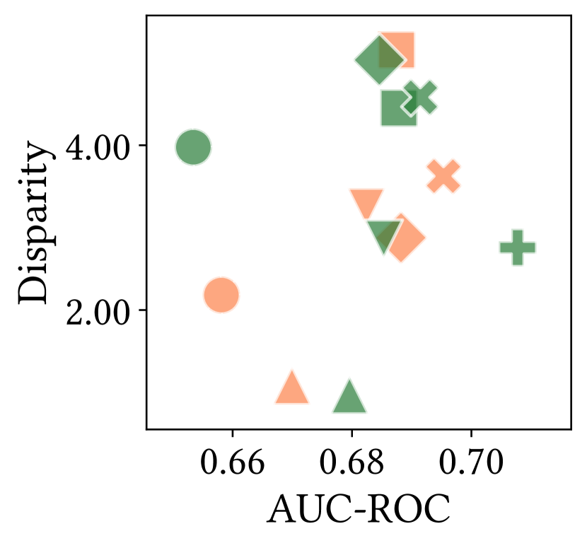
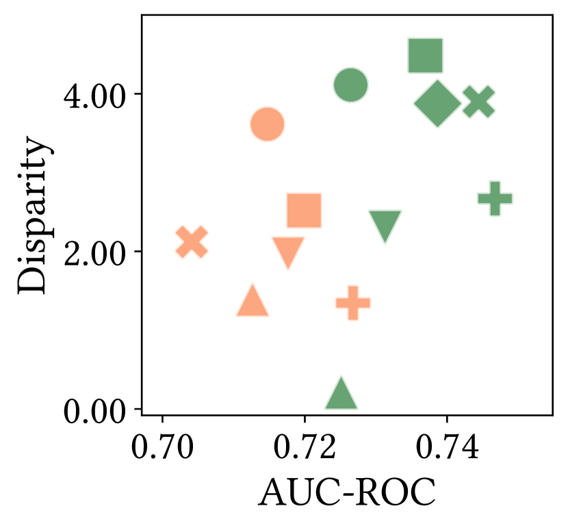
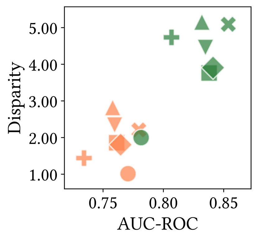
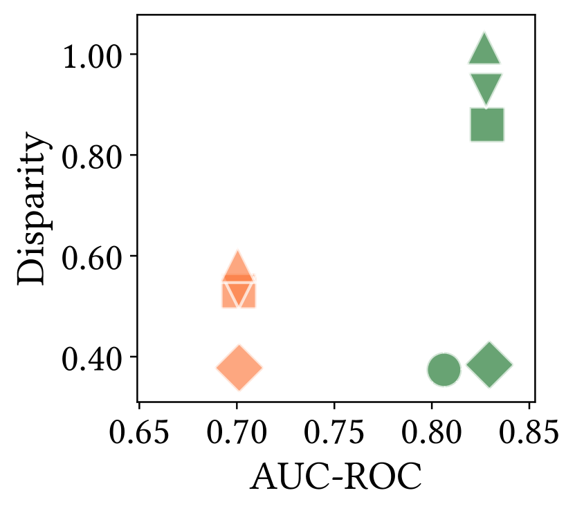
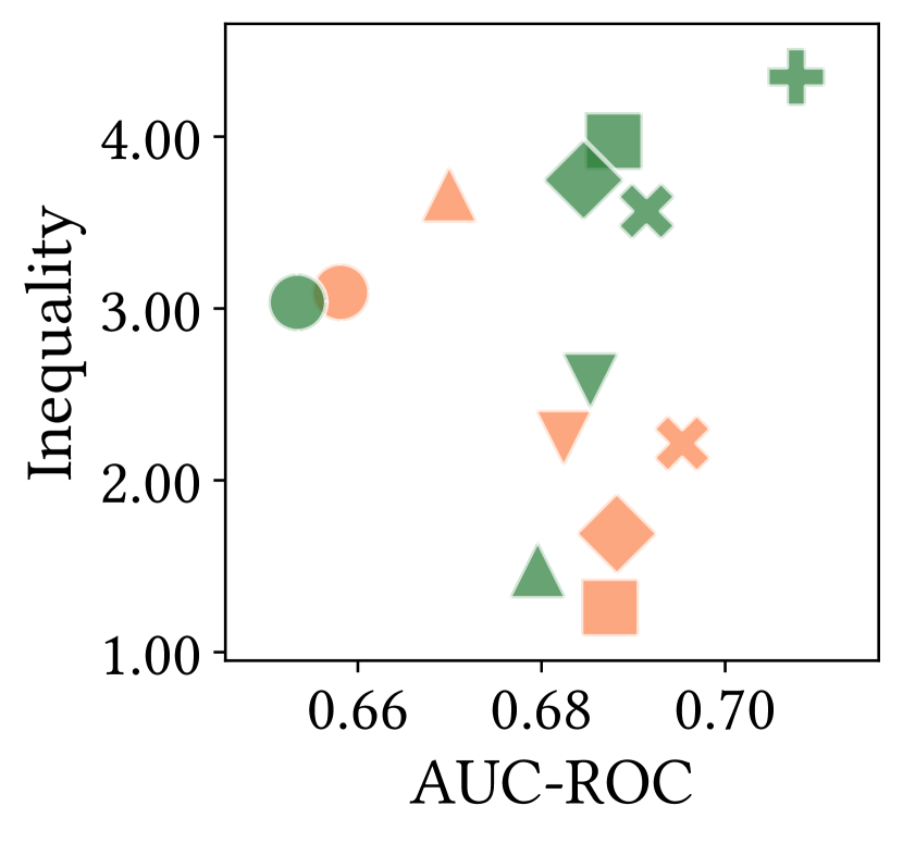
(a) German

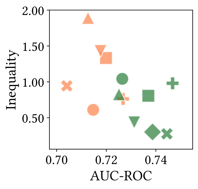
(b) Credit

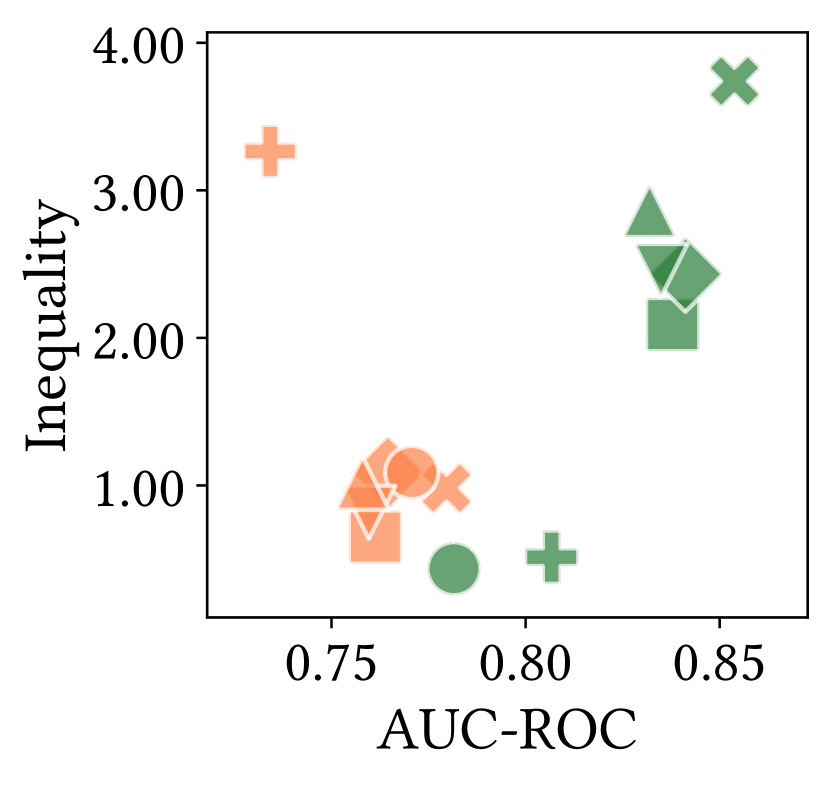
(c) Penn94

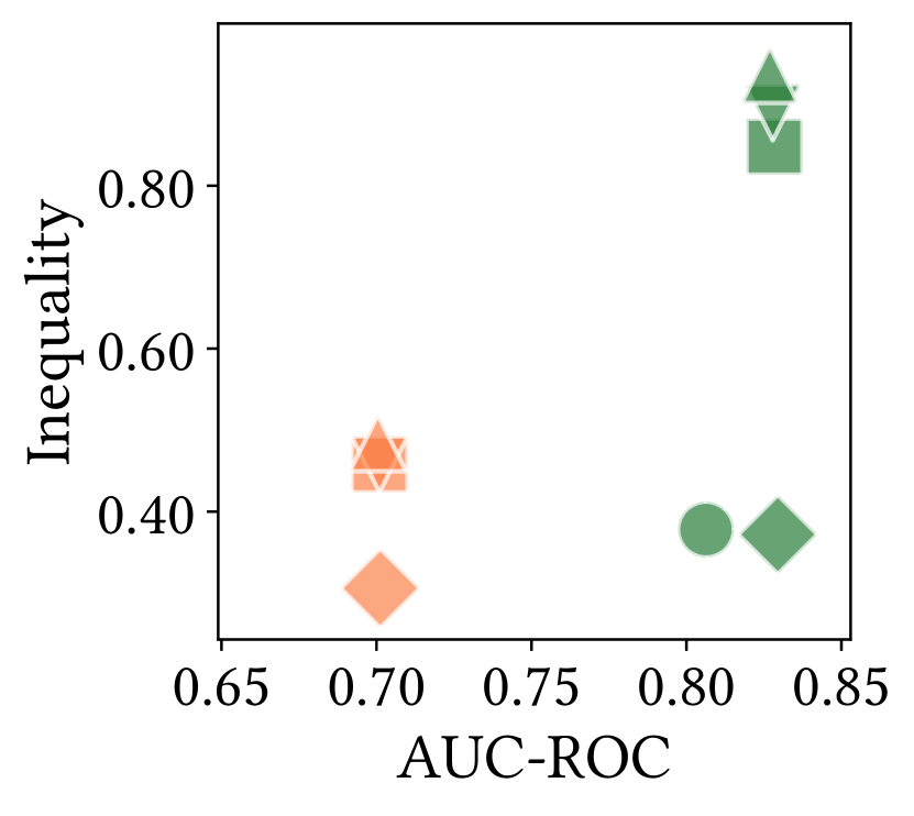
(d) Pokec-z

Figure 1. Accuracy (X-axis, larger is better) measured using AUC-ROC versus algorithmic discrimination (Y-axis, smaller is better) measured using Disparity (top row) and Inequality (bottom row) reported as percentages. The optimal is towards the bottom right in all plots which denotes higher AUC-ROC and lower Disparity and Equality.

5.2. Methodology

Processing Datasets.

Agarwal et al. (2021) and Dong et al. (2022) utilize a non-standardized method for creating dataset splits that does not include all nodes. Following convention, we create new stratified random splits such that the label imbalance in the original data is reflected in each of the training, validation, and test sets. For German, Credit, and Pokec-z, we use 60% of the dataset for training, 20% for validation, and the remaining 20% for testing. For Penn94, we use only 20% for training and validation (each) because we find that is sufficient for GNNs, with the remaining 60% used for testing. Additionally, we adapt the datasets for use by PFR as described previously (cf. Section 4.1). For computing between-group quantile graphs, we choose Loan Amount, Maximum Bill Amount Over Last 6 Months, Spoken Language, and F6 as ranking variables for German, Credit, Pokec-z, and Penn94 respectively.

Interventions.

Each intervention in our study is benchmarked against the performance of three vanilla GNNs namely, GCN, GraphSAGE, and GIN, referred to as Original. We construct PFR-AX to debias $\mathbf{X}$ and $\mathbf{A}$ as per Section 4.1. For ablation, we consider two variants: (i) PFR-X that only applies PFR on $\mathbf{X}$, (ii) PFR-A that applies only PFR on a DeepWalk embedding and reconstructs a graph using EmbeddingReverser.

We vary $\gamma$ from 0.1 (1%) to 0.4 (40%) in increments of 0.1. For each $\gamma$, we use the same hyperparameters that returned the maximum accuracy for vanilla GNNs and post-process their predictions as per Algorithm 2. For each seed and $\gamma$, we randomly select $\gamma$ fraction of nodes from the protected class with a predicted negative outcome and smoothen over 20 trials. We define heavy and light versions of PostProcess namely, (i) PostProcess+ and (ii) PostProcess-, in terms of $\gamma$. PostProcess+ is defined at that value of $\gamma$ where disparity is lowest compared to Original and PostProcess- is set halfway between the disparity of Original and PostProcess+.

We compare these with three baselines: (i) Unaware (that naively deletes the sensitive attribute column from $\mathbf{X}$), (ii) EDITS (Dong et al., 2022), and (iii) NIFTY (Agarwal et al., 2021). Previous studies do not consider Unaware which is a competitive baseline according to our results (see below).

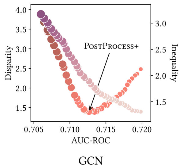
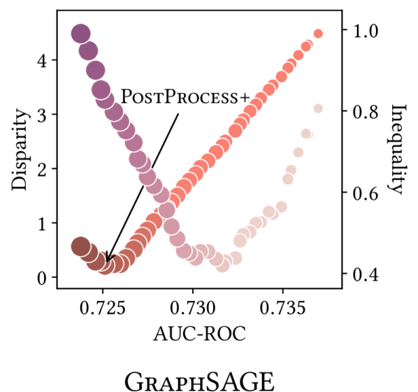
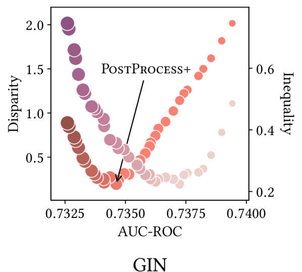
Figure 2. AUC-ROC as a function of Disparity (red) and Inequality (purple) for varying levels of the $\gamma$ parameter of PostProcess on the Credit dataset. Higher values of $\gamma$ are depicted by larger marker shapes and darker colors and indicate heavier interventions. As $\gamma$ increases, AUC-ROC always decreases and Equality increases. Disparity first decreases upto an inflection point and then increases indicating an over-correction towards the protected class.

(a) GCN

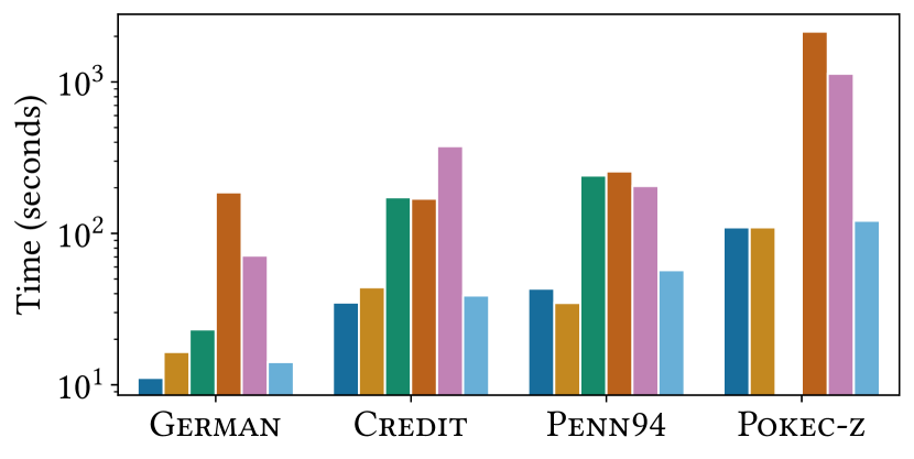
(b) GraphSAGE

(c) GIN

Figure 3. Runtime in seconds (log-scale) of various interventions on GCN, GraphSAGE, and GIN for German, Credit, Penn94, and Pokec-z increasing with dataset size. PostProcess is fastest because updating model inference is inexpensive.

Training.

We set $k=128$ dimensions for DeepWalk. Depending on the dataset and interventions, we allow models to train for 500, 1000, 1500, or 2000 epochs. As per convention, we report results for each model/intervention obtained after $T$ epochs and averaged over 5 runs. This is different from previous studies such as NIFTY that train for (say) $T$ epochs and report results for that model instance that has the best validation score from upto $T$ epochs. This, combined with our stratified splits, is a key factor for observing materially different scores from those reported by the original authors. To ensure fair comparison, we tune hyperparameters for each intervention and model via a combination of manual grid search and Bayesian optimization using WandB (Biewald, 2020). The goal of this hyperparameter optimization is to find that setting of hyperparameters that results in a model with a maximal AUC-ROC score while aiming to have lower disparity and equality scores than Original.

Implementation.

We implement our models and interventions in Python 3.7. We use SNAP’s C++ implementation for DeepWalk. EDITS and NIFTY are adapted from their original implementations. Our experiments were conducted on a Linux machine with 32 cores, 100 GB RAM, and an V100 GPU. Our code is available at https://github.com/arpitdm/gnn_accuracy_fairness_tradeoff.

5.3. Results

Algorithmic Fairness-Accuracy Tradeoff.

Figure 1 presents AUC-ROC (X-axis) against disparity (Y-axis) in the first row and inequality (Y-axis) in the second row achieved by various interventions for the four datasets (cf. RQ1). We represent the vanilla GCN model as an orange square and use different orange markers for different interventions on GCN. GraphSAGE is similarly illustrated in green. Interventions that cause a $>5\%$ (multiplicative) decrease in AUC-ROC compared to the vanilla model are omitted from the plot. Since higher values of AUC-ROC and lower values of $\Delta_{\text{SP}}$ and $\Delta_{\text{EO}}$ are better, the optimal position is towards the bottom right in each plot (cf. RQ2). For ease of presentation, we defer full results for GIN and all interventions to Table 2 in Appendix A.

Across datasets, GraphSAGE and GIN are more accurate than GCN but GraphSAGE displays higher disparity and inequality while GIN displays lower. PFR-AX and PostProcess- offer better tradeoffs than other baselines for German and Credit across models. This translates to upto 70% and 80% lower disparity than Original at less than 5% and 1% decrease in accuracy on German, respectively. In comparison, NIFTY offers 60% lower disparity (2.18% vs. 5.16% on German) at a 4.22% reduction in AUC-ROC. The lack of correlation between decreases in disparity and inequality may be explained in part by the impossibility theorem showing that these two criteria cannot be optimized simultaneously Chouldechova (2017). In Penn94 and Pokec-z, PFR-A and PFR-X are more effective than PFR-AX (cf. Table 2). We caveat the use of PostProcess in these datasets because choosing nodes randomly displays unintended consequences in maintaining accuracy without promoting fairness. Unaware proves effective across models and is especially optimal for Pokec-z. EDITS proves a heavy intervention causing large reductions in accuracy for relatively small gains in disparity.

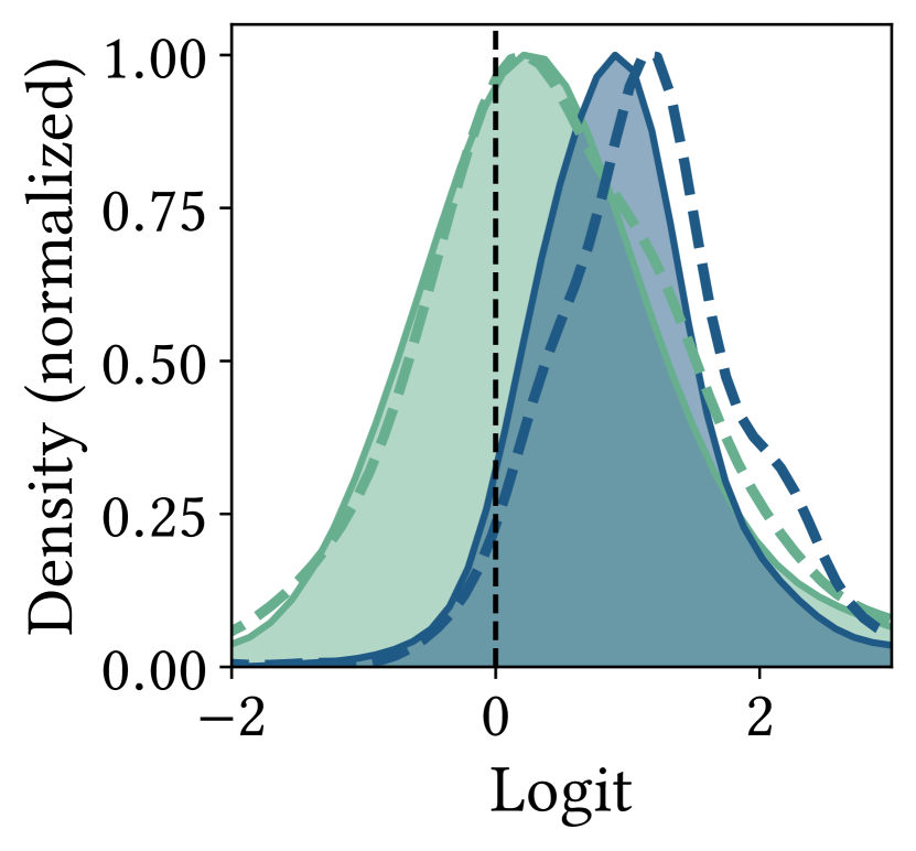
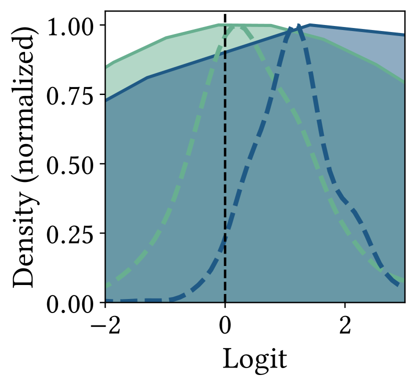
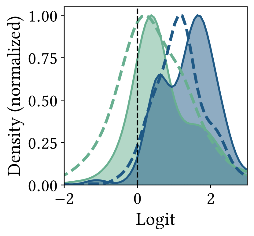
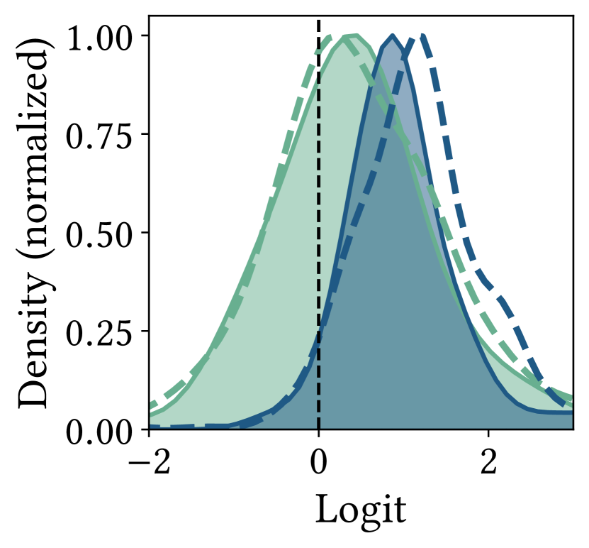
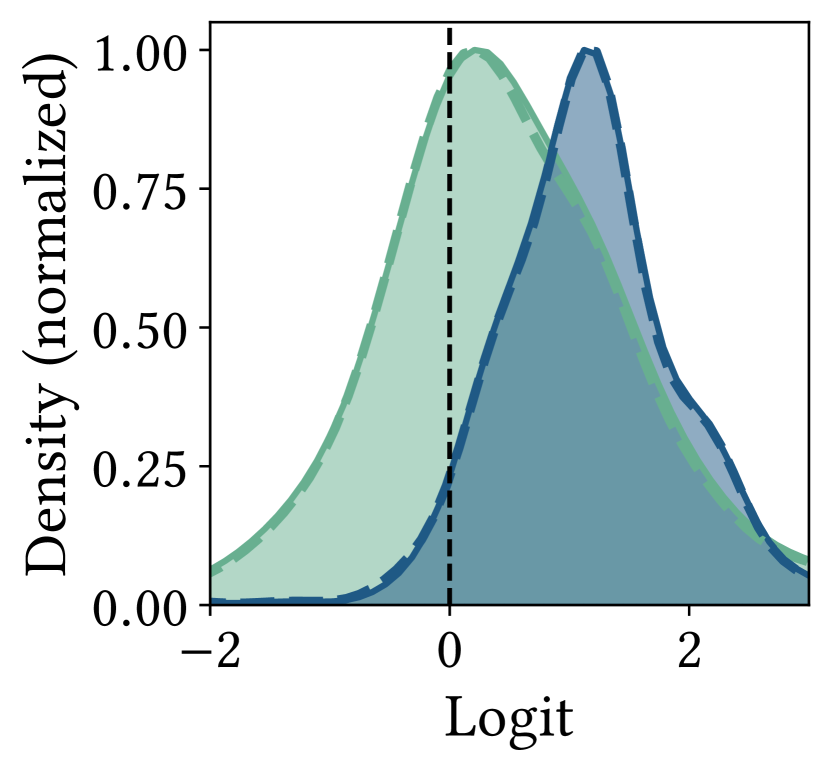
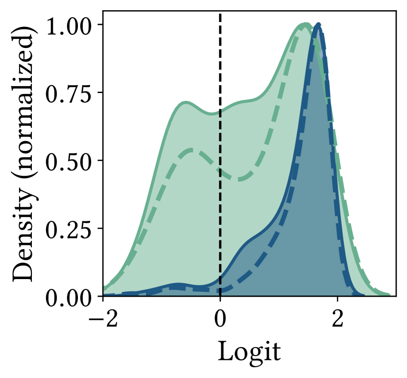
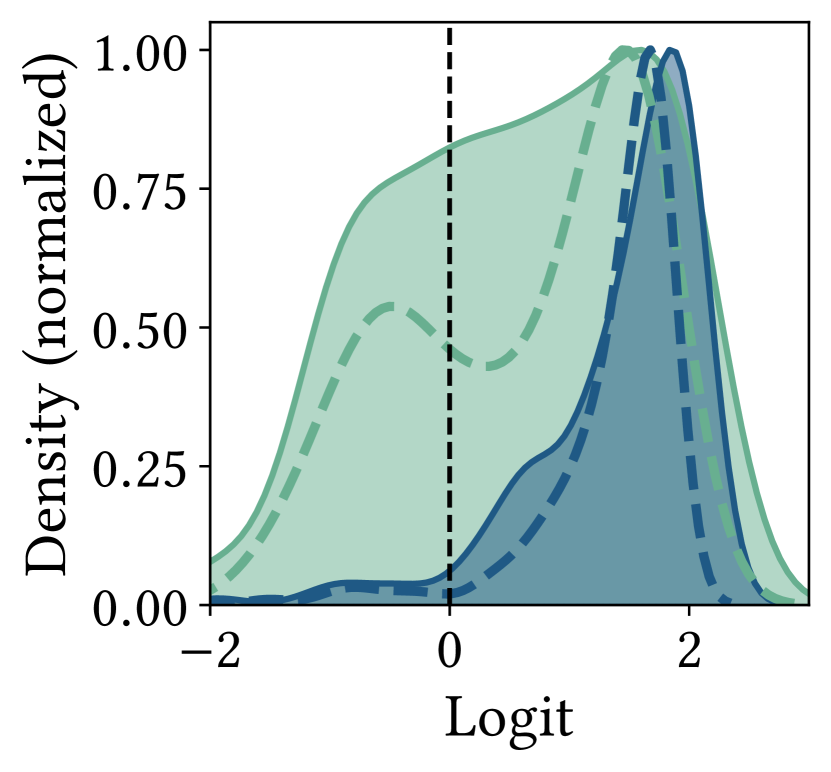
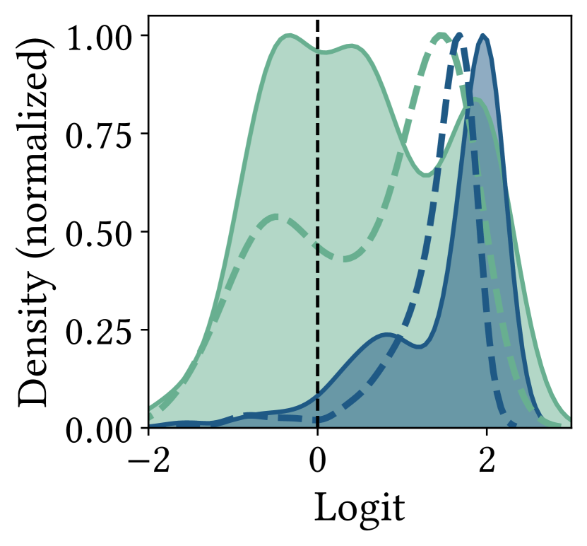
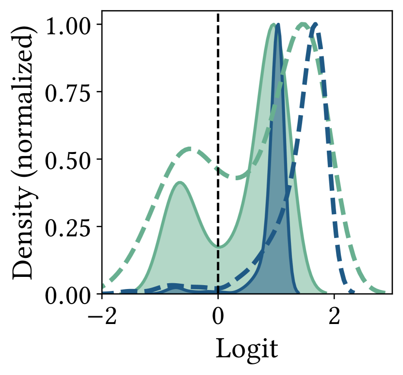
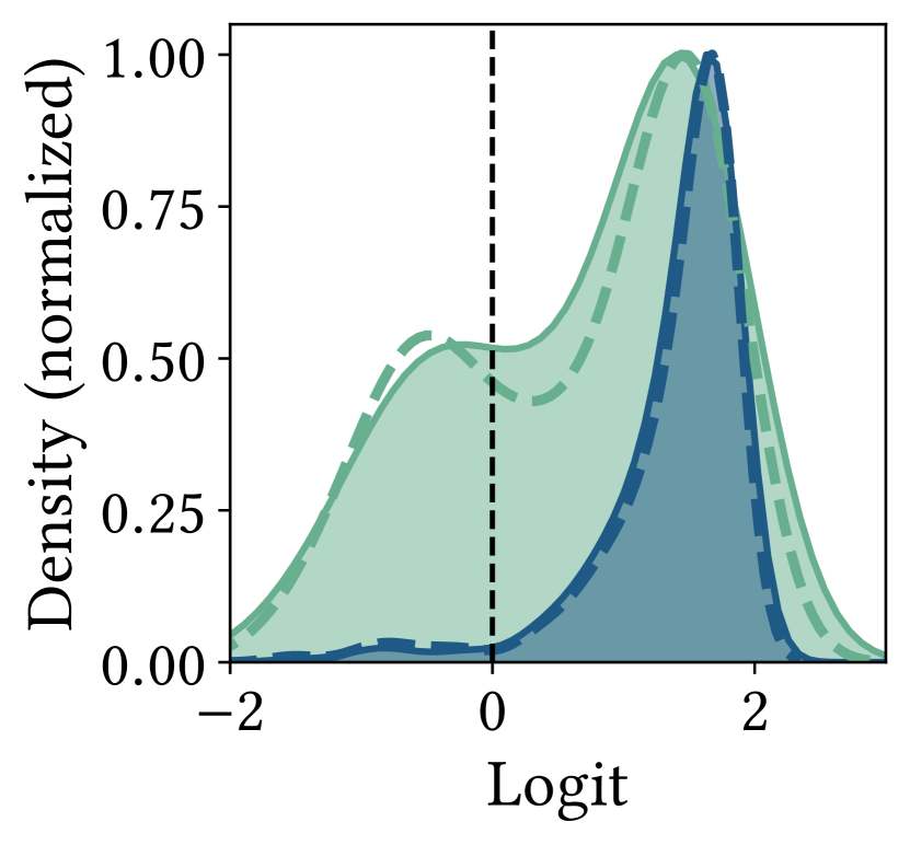
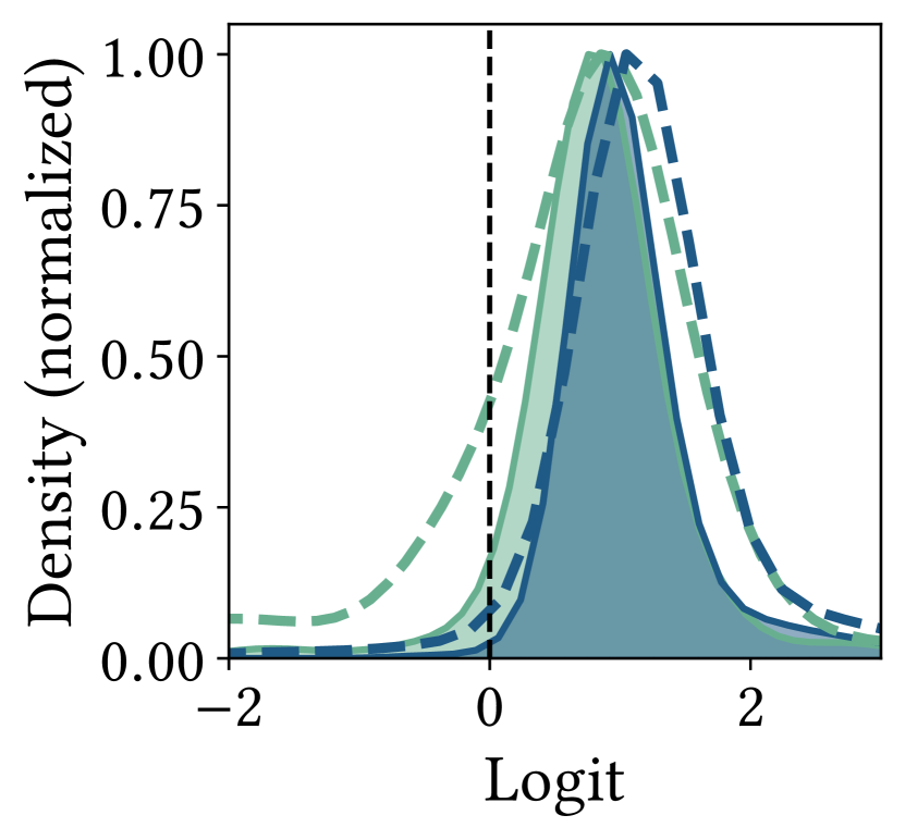
(a) Unaware

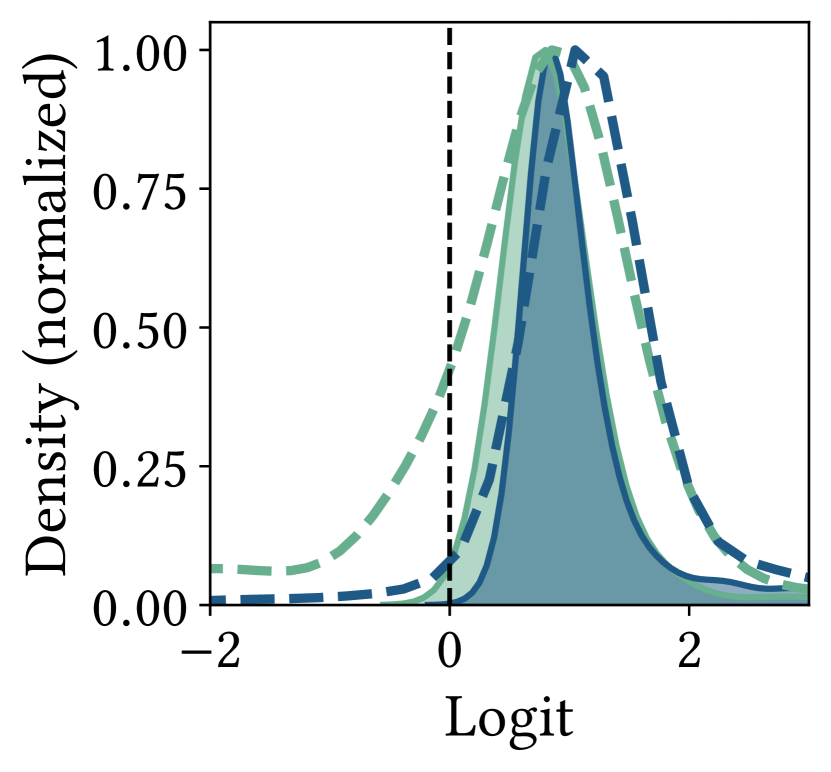
(b) EDITS

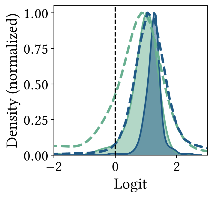
(c) PFR-AX

(d) NIFTY

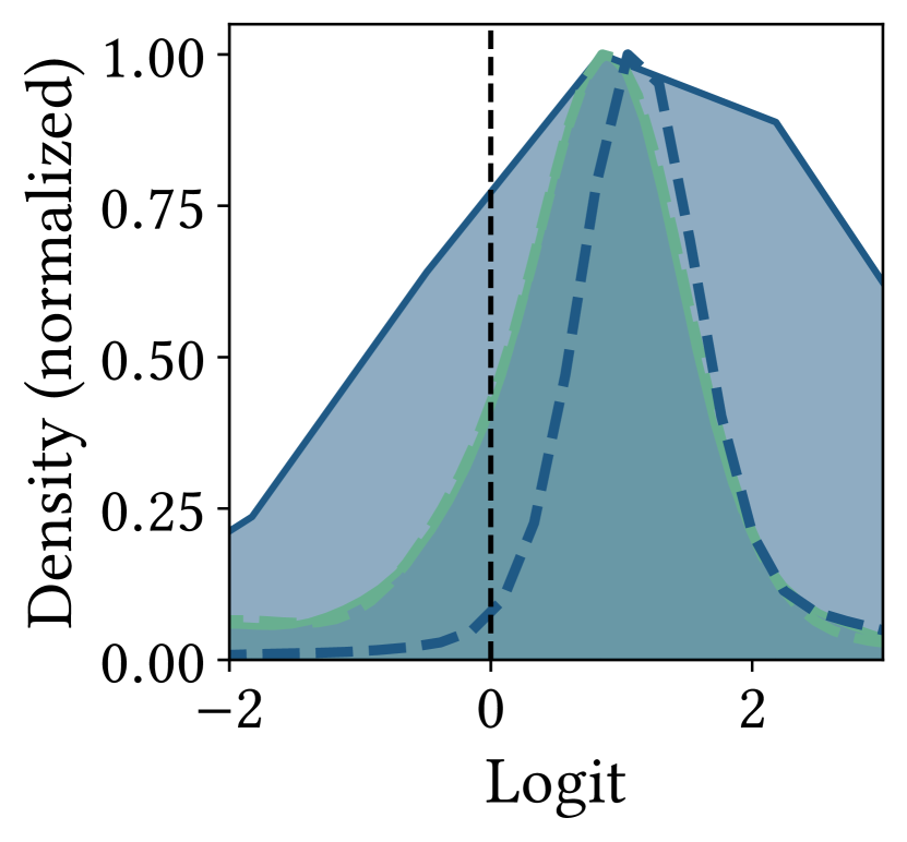
(e) PostProcess-

Figure 4. Density of logit scores of GCN (first row), GraphSAGE (second row), and GIN (third row) after applying different algorithmic fairness interventions for users in the protected class in the Credit dataset. The vertical dashed (black) line depicts the threshold used for label prediction (positive scores indicate positive outcomes). The colored dashed curves indicate the density of output scores of Original. PFR-AX and PostProcess- improve model confidence (density) for correctly predicting a positive label for users in the protected class.

Sensitivity to $\gamma$.

Figure 2 trades off AUC (X-axis), disparity (left Y-axis, red points), and inequality (right Y-axis, purple points) for GCN, GraphSAGE, and GIN on Credit as a function of $\gamma$. Due to large label imbalance in Credit and small number of nodes with negative predicted outcomes from the protected class, varying $\gamma$ by 1% translates to changing predictions for 7 nodes. PostProcess thus offers granular control. As $\gamma$ increases, AUC-ROC decreases while $\Delta_{\text{SP}}$ first reduces and then increases again. This inflection point indicates that the post-processing policy is overcorrecting in favour of the protected class resulting in disparity towards the non-protected class. Conversely, such improvements are absent in Pokec-z since vanilla GNNs themselves are inherently less biased.

Runtime.

Figure 3 depicts the total computation time in seconds (on log-scale) for each intervention on the four datasets for GCN, GraphSAGE, and GIN. We observe similar trends for all three GNN models. As expected, the larger the dataset, the higher the runtime. Updating a model’s predictions at inference time is inexpensive and the resulting overhead for PostProcess is thus negligible. The running time for PFR-AX increases significantly with increasing dataset size. The key bottlenecks are very eigenvalue decompositions for sparse, symmetric matrices in PFR requiring $\mathcal{O}\left(n^{3}\right)$ time and constructing DeepWalk embeddings. For instance, in the case of Pokec-z, PFR required (on average) 47 minutes in our tests while EmbeddingReverser and GNN training required less than 5 minutes each. For comparison, NIFTY required approximately 22 minutes while EDITS did not complete due to memory overflow.

Model Confidence.

In Figure 4, we display the impact of fairness interventions on a model’s confidence about its predictions, i.e., uncalibrated density (Y-axis), compared to its logit scores (X-axis) on the Credit dataset. The plots in the top, middle, and bottom rows corresponds to GCN, GraphSAGE, and GIN, respectively. Larger positive values imply higher confidence about predicting a positive outcome and larger negative values imply higher confidence for a negative outcome prediction. While there isn’t a universal desired outcome, an intermediate goal for an intervention may be to ensure that a model is equally confident about correctly predicting both positive and negative labels. Blue regions show normalized density of logit values for nodes in the protected class with a positive ground-truth label (S1-Y1) and green regions show the same for nodes in the protected class with a negative outcome as ground-truth. The dashed colored lines indicate density values for these groups of nodes for the Original model. PostProcess and Unaware induce small changes to GNN’s outputs while EDITS is significantly disruptive. PFR-AX nudges the original model’s output for nodes in S1-Y1 away from 0 making it more confident about its positive (correct) predictions while NIFTY achieves the reverse.

6. Conclusion

We presented two interventions that intrinsically differ from existing methods: PFR-AX debiases data prior to training to connect similar nodes across protected and non-protected groups while seeking to preserve existing degree distributions; PostProcess updates model predictions to reduce error rates across protected user groups. We frame our study in the context of the tension between disparity, inequality, and accuracy and quantify the scope for improvements and show that our approaches offer intuitive control over this tradeoff. Given their model-agnostic nature, we motivate future analysis by combining multiple interventions at different loci in the learning pipeline.

Appendix A Additional Experimental Results

Table 2. Accuracy (AUC-ROC) and algorithmic fairness (Disparity and Inequality) scores for 8 interventions for GCN, GraphSAGE, and GIN models on four datasets. Results are averaged across five runs. Higher values of AUC (fraction between 0 and 1) indicate higher performance. Lower values of disparity ($\Delta_{\text{SP}}$) and inequality ($\Delta_{\text{EO}}$) in percentage indicate higher algorithmic fairness. No single intervention dominates all others across datasets and models. However, PostProcess- generally offers a gentle accuracy-fairness tradeoff. A dashed line denotes out-of-memory.

Dataset	Model	Metric	Original	Unaware	EDITS	PFR-A	PFR-X	PFR-AX	NIFTY	PostProcess+	PostProcess-
German	GCN	AUC-ROC	0.687	0.688	0.695	0.643	0.698	0.638	0.658	0.670	0.682
		Parity	5.156	2.878	3.625	2.068	4.204	3.878	2.182	1.082	3.250
		Equality	1.260	1.690	2.215	1.54	2.612	2.112	3.094	3.668	2.242
	GraphSAGE	AUC-ROC	0.688	0.685	0.691	0.665	0.708	0.708	0.653	0.680	0.685
		Parity	4.450	5.034	4.582	2.856	3.072	2.758	3.976	0.970	2.864
		Equality	3.974	3.748	3.566	2.804	5.174	4.348	3.036	1.482	2.576
	GIN	AUC-ROC	0.709	0.707	0.675	0.664	0.619	0.59	0.654	0.680	0.696
		Parity	8.600	1.496	5.61	2.714	1.218	2.602	2.118	2.882	6.058
		Equality	2.168	4.260	2.824	1.6	1.362	4.476	3.278	2.216	1.624
Credit	GCN	AUC-ROC	0.720	0.681	0.704	0.721	0.735	0.727	0.715	0.713	0.718
		Parity	2.518	6.194	2.12	3.094	0.316	1.344	3.614	1.396	1.962
		Equality	1.332	4.550	0.944	1.274	0.444	0.762	0.610	1.890	1.430
	GraphSAGE	AUC-ROC	0.737	0.739	0.744	0.72	0.751	0.747	0.726	0.725	0.731
		Parity	4.484	3.876	3.9	3.866	2.746	2.67	4.112	0.218	2.298
		Equality	0.806	0.302	0.276	1.184	0.366	0.98	1.042	0.828	0.436
	GIN	AUC-ROC	0.739	0.713	0.707	0.724	0.742	0.716	0.716	0.735	0.737
		Parity	2.016	0.686	0.86	1.32	0.612	1.616	3.268	0.194	1.142
		Equality	0.486	0.296	0.494	1.204	0.776	0.416	0.440	0.358	0.224
Penn94	GCN	AUC-ROC	0.761	0.765	0.78	0.69	0.796	0.734	0.771	0.758	0.760
		Parity	1.858	1.806	2.208	1.856	1.21	1.44	1.014	2.820	2.340
		Equality	0.650	1.086	0.982	3.046	2.254	3.264	1.088	1.016	0.818
	GraphSAGE	AUC-ROC	0.838	0.841	0.854	0.732	0.83	0.807	0.782	0.832	0.835
		Parity	3.762	3.908	5.09	2.54	4.326	4.734	1.998	5.154	4.456
		Equality	2.090	2.432	3.74	0.922	1.692	0.514	0.436	2.864	2.456
	GIN	AUC-ROC	0.789	0.778	0.776	0.717	0.694	0.731	0.769	0.784	0.786
		Parity	1.546	1.058	1.474	1.081	1.670	1.182	0.862	3.116	2.320
		Equality	2.358	1.732	3.306	4.584	2.672	2.368	1.966	1.130	1.732
Pokec-Z	GCN	AUC-ROC	0.701	0.701	–	0.66	0.616	0.615	0.627	0.700	0.701
		Parity	0.530	0.378	–	0.235	0.216	0.502	0.700	0.582	0.530
		Equality	0.458	0.306	–	0.412	0.078	0.486	0.582	0.484	0.458
	GraphSAGE	AUC-ROC	0.828	0.830	–	0.827	0.775	0.778	0.806	0.827	0.828
		Parity	0.860	0.384	–	0.954	0.33	0.327	0.374	1.014	0.928
		Equality	0.848	0.372	–	0.634	0.464	0.458	0.378	0.936	0.890
	GIN	AUC-ROC	0.712	0.710	–	0.651	0.623	0.641	0.669	0.712	0.712
		Parity	0.406	0.136	–	0.721	0.181	0.673	0.156	0.456	0.406
		Equality	0.398	0.076	–	1.898	1.439	1.887	0.114	0.438	0.398

References

- (1)
- Agarwal et al. (2021) Chirag Agarwal, Himabindu Lakkaraju, and Marinka Zitnik. 2021. Towards a unified framework for fair and stable graph representation learning. In Uncertainty in Artificial Intelligence. PMLR, 2114–2124.
- Barocas and Selbst (2016) Solon Barocas and Andrew D Selbst. 2016. Big Data’s Disparate Impact. California law review 104, 3 (2016), 671–732.
- Biewald (2020) Lukas Biewald. 2020. Experiment Tracking with Weights and Biases. https://www.wandb.com/ Software available from wandb.com.
- Chouldechova (2017) Alexandra Chouldechova. 2017. Fair prediction with disparate impact: A study of bias in recidivism prediction instruments. Big data 5, 2 (2017), 153–163.
- Corbett-Davies et al. (2017) Sam Corbett-Davies, Emma Pierson, Avi Feller, Sharad Goel, and Aziz Huq. 2017. Algorithmic Decision Making and the Cost of Fairness. In Proceedings of the 23rd ACM SIGKDD International Conference on Knowledge Discovery and Data Mining (Halifax, NS, Canada) (KDD ’17). Association for Computing Machinery, New York, NY, USA, 797–806. https://doi.org/10.1145/3097983.3098095
- Dai and Wang (2021) Enyan Dai and Suhang Wang. 2021. Say No to the Discrimination: Learning Fair Graph Neural Networks with Limited Sensitive Attribute Information. In Proceedings of the 14th ACM International Conference on Web Search and Data Mining (Virtual Event, Israel) (WSDM ’21). Association for Computing Machinery, New York, NY, USA, 680–688. https://doi.org/10.1145/3437963.3441752
- Dai et al. (2022) Enyan Dai, Tianxiang Zhao, Huaisheng Zhu, Junjie Xu, Zhimeng Guo, Hui Liu, Jiliang Tang, and Suhang Wang. 2022. A Comprehensive Survey on Trustworthy Graph Neural Networks: Privacy, Robustness, Fairness, and Explainability. arXiv preprint arXiv:2204.08570 (2022).
- Dong et al. (2021) Yushun Dong, Jian Kang, Hanghang Tong, and Jundong Li. 2021. Individual Fairness for Graph Neural Networks: A Ranking Based Approach. In Proceedings of the 27th ACM SIGKDD Conference on Knowledge Discovery &; Data Mining (Virtual Event, Singapore) (KDD ’21). Association for Computing Machinery, New York, NY, USA, 300–310. https://doi.org/10.1145/3447548.3467266
- Dong et al. (2022) Yushun Dong, Ninghao Liu, Brian Jalaian, and Jundong Li. 2022. EDITS: Modeling and Mitigating Data Bias for Graph Neural Networks. In Proceedings of the ACM Web Conference 2022 (Virtual Event, Lyon, France) (WWW ’22). Association for Computing Machinery, New York, NY, USA, 1259–1269. https://doi.org/10.1145/3485447.3512173
- Dua and Graff (2017) Dheeru Dua and Casey Graff. 2017. UCI Machine Learning Repository. http://archive.ics.uci.edu/ml
- Dwork et al. (2012) Cynthia Dwork, Moritz Hardt, Toniann Pitassi, Omer Reingold, and Richard Zemel. 2012. Fairness through Awareness. In Proceedings of the 3rd Innovations in Theoretical Computer Science Conference (Cambridge, Massachusetts) (ITCS ’12). Association for Computing Machinery, New York, NY, USA, 214–226. https://doi.org/10.1145/2090236.2090255
- Elazar and Goldberg (2018) Yanai Elazar and Yoav Goldberg. 2018. Adversarial Removal of Demographic Attributes from Text Data. In Proceedings of the 2018 Conference on Empirical Methods in Natural Language Processing. Association for Computational Linguistics, Brussels, Belgium, 11–21. https://doi.org/10.18653/v1/D18-1002
- Fish et al. (2016) Benjamin Fish, Jeremy Kun, and Ádám D Lelkes. 2016. A confidence-based approach for balancing fairness and accuracy. In Proceedings of the 2016 SIAM international conference on data mining. SIAM, 144–152.
- Gao et al. (2020) Yang Gao, Hong Yang, Peng Zhang, Chuan Zhou, and Yue Hu. 2020. Graph Neural Architecture Search. In Proceedings of the Twenty-Ninth International Joint Conference on Artificial Intelligence, IJCAI-20, Christian Bessiere (Ed.). International Joint Conferences on Artificial Intelligence Organization, 1403–1409. https://doi.org/10.24963/ijcai.2020/195 Main track.
- Hamilton et al. (2017) William L. Hamilton, Rex Ying, and Jure Leskovec. 2017. Representation Learning on Graphs: Methods and Applications. (2017), 1–24. arXiv:1709.05584 http://arxiv.org/abs/1709.05584
- Hardt et al. (2016) Moritz Hardt, Eric Price, Eric Price, and Nati Srebro. 2016. Equality of Opportunity in Supervised Learning. In Advances in Neural Information Processing Systems, D. Lee, M. Sugiyama, U. Luxburg, I. Guyon, and R. Garnett (Eds.), Vol. 29. Curran Associates, Inc. https://proceedings.neurips.cc/paper/2016/file/9d2682367c3935defcb1f9e247a97c0d-Paper.pdf
- Jin et al. (2020) Guangyin Jin, Qi Wang, Cunchao Zhu, Yanghe Feng, Jincai Huang, and Jiangping Zhou. 2020. Addressing Crime Situation Forecasting Task with Temporal Graph Convolutional Neural Network Approach. In 12th International Conference on Measuring Technology and Mechatronics Automation. IEEE Computer Society, Los Alamitos, CA, USA, 474–478. https://doi.org/10.1109/ICMTMA50254.2020.00108
- Kamiran and Calders (2012) Faisal Kamiran and Toon Calders. 2012. Data preprocessing techniques for classification without discrimination. Knowledge and Information Systems 33, 1 (2012), 1–33. https://doi.org/10.1007/s10115-011-0463-8
- Khajehnejad et al. (2022) Ahmad Khajehnejad, Moein Khajehnejad, Mahmoudreza Babaei, Krishna P Gummadi, Adrian Weller, and Baharan Mirzasoleiman. 2022. CrossWalk: fairness-enhanced node representation learning. In Proceedings of the AAAI Conference on Artificial Intelligence, Vol. 36. 11963–11970.
- Kipf and Welling (2017) Thomas N. Kipf and Max Welling. 2017. Semi-Supervised Classification with Graph Convolutional Networks. In International Conference on Learning Representations (ICLR).
- Kleinberg et al. (2019) Jon Kleinberg, Jens Ludwig, Sendhil Mullainathan, and Cass R Sunstein. 2019. Discrimination in the Age of Algorithms. Journal of Legal Analysis 10 (04 2019), 113–174. https://doi.org/10.1093/jla/laz001
- Lahoti et al. (2020) Preethi Lahoti, Krishna P. Gummadi, and Gerhard Weikum. 2020. Operationalizing Individual Fairness with Pairwise Fair Representations. Proc. VLDB Endow. 13, 4 (jan 2020), 506–518. https://doi.org/10.14778/3372716.3372723
- Li et al. (2018) Qimai Li, Zhichao Han, and Xiao-Ming Wu. 2018. Deeper insights into graph convolutional networks for semi-supervised learning. In Proceedings of the AAAI Conference on Artificial Intelligence, Vol. 32.
- Liang et al. (2022) Annie Liang, Jay Lu, and Xiaosheng Mu. 2022. Algorithmic Design: Fairness Versus Accuracy. In Proceedings of the 23rd ACM Conference on Economics and Computation (Boulder, CO, USA) (EC ’22). Association for Computing Machinery, New York, NY, USA, 58–59. https://doi.org/10.1145/3490486.3538237
- Lim et al. (2021) Derek Lim, Felix Hohne, Xiuyu Li, Sijia Linda Huang, Vaishnavi Gupta, Omkar Bhalerao, and Ser Nam Lim. 2021. Large scale learning on non-homophilous graphs: New benchmarks and strong simple methods. Advances in Neural Information Processing Systems 34 (2021), 20887–20902.
- Lipton et al. (2018) Zachary Lipton, Julian McAuley, and Alexandra Chouldechova. 2018. Does mitigating MLs impact disparity require treatment disparity?. In Advances in Neural Information Processing Systems, S. Bengio, H. Wallach, H. Larochelle, K. Grauman, N. Cesa-Bianchi, and R. Garnett (Eds.), Vol. 31. Curran Associates, Inc. https://proceedings.neurips.cc/paper/2018/file/8e0384779e58ce2af40eb365b318cc32-Paper.pdf
- Liu and Avci (2019) Frederick Liu and Besim Avci. 2019. Incorporating priors with feature attribution on text classification. arXiv preprint arXiv:1906.08286 (2019).
- Menon and Williamson (2018) Aditya Krishna Menon and Robert C Williamson. 2018. The cost of fairness in binary classification. In Proceedings of the 1st Conference on Fairness, Accountability and Transparency (Proceedings of Machine Learning Research, Vol. 81), Sorelle A. Friedler and Christo Wilson (Eds.). PMLR, 107–118. https://proceedings.mlr.press/v81/menon18a.html
- Perozzi et al. (2014) Bryan Perozzi, Rami Al-Rfou, and Steven Skiena. 2014. DeepWalk: Online Learning of Social Representations. In Proceedings of the 20th ACM SIGKDD International Conference on Knowledge Discovery and Data Mining (KDD ’14). ACM, New York, NY, USA, 701–710.
- Raghavan et al. (2020) Manish Raghavan, Solon Barocas, Jon Kleinberg, and Karen Levy. 2020. Mitigating Bias in Algorithmic Hiring: Evaluating Claims and Practices. In Proceedings of the 2020 Conference on Fairness, Accountability, and Transparency (Barcelona, Spain) (FAT* ’20). Association for Computing Machinery, New York, NY, USA, 469–481. https://doi.org/10.1145/3351095.3372828
- Song et al. (2022) Weihao Song, Yushun Dong, Ninghao Liu, and Jundong Li. 2022. GUIDE: Group Equality Informed Individual Fairness in Graph Neural Networks. In Proceedings of the 28th ACM SIGKDD Conference on Knowledge Discovery and Data Mining (Washington DC, USA) (KDD ’22). Association for Computing Machinery, New York, NY, USA, 1625–1634. https://doi.org/10.1145/3534678.3539346
- Stephanopoulos (2018) Nicholas O Stephanopoulos. 2018. Disparate Impact, Unified Law. Yale LJ 128 (2018), 1566.
- Traud et al. (2012) Amanda L. Traud, Peter J. Mucha, and Mason A. Porter. 2012. Social structure of Facebook networks. Physica A: Statistical Mechanics and its Applications 391, 16 (2012), 4165–4180. https://doi.org/10.1016/j.physa.2011.12.021
- Ustun et al. (2019) Berk Ustun, Alexander Spangher, and Yang Liu. 2019. Actionable Recourse in Linear Classification. In Proceedings of the Conference on Fairness, Accountability, and Transparency (Atlanta, GA, USA) (FAT* ’19). Association for Computing Machinery, New York, NY, USA, 10–19. https://doi.org/10.1145/3287560.3287566
- Wei et al. (2020) Dennis Wei, Karthikeyan Natesan Ramamurthy, and Flavio Calmon. 2020. Optimized Score Transformation for Fair Classification. In Proceedings of the Twenty Third International Conference on Artificial Intelligence and Statistics (Proceedings of Machine Learning Research, Vol. 108), Silvia Chiappa and Roberto Calandra (Eds.). PMLR, 1673–1683. https://proceedings.mlr.press/v108/wei20a.html
- Xiao et al. (2022) Shunxin Xiao, Shiping Wang, Yuanfei Dai, and Wenzhong Guo. 2022. Graph neural networks in node classification: survey and evaluation. Machine Vision and Applications 33, 1 (2022), 1–19.
- Xu et al. (2018) Keyulu Xu, Weihua Hu, Jure Leskovec, and Stefanie Jegelka. 2018. How powerful are graph neural networks? arXiv preprint arXiv:1810.00826 (2018).
- Zafar et al. (2017) Muhammad Bilal Zafar, Isabel Valera, Manuel Gomez Rodriguez, and Krishna P. Gummadi. 2017. Fairness Beyond Disparate Treatment &; Disparate Impact: Learning Classification without Disparate Mistreatment. In Proceedings of the 26th International Conference on World Wide Web (Perth, Australia) (WWW ’17). International World Wide Web Conferences Steering Committee, Republic and Canton of Geneva, CHE, 1171–1180. https://doi.org/10.1145/3038912.3052660
- Zemel et al. (2013) Rich Zemel, Yu Wu, Kevin Swersky, Toni Pitassi, and Cynthia Dwork. 2013. Learning fair representations. In International conference on machine learning. PMLR, 325–333.
- Zeng et al. (2020) Hanqing Zeng, Hongkuan Zhou, Ajitesh Srivastava, Rajgopal Kannan, and Viktor Prasanna. 2020. GraphSAINT: Graph Sampling Based Inductive Learning Method. In International Conference on Learning Representations. https://openreview.net/forum?id=BJe8pkHFwS
- Zhu et al. (2020) Jiong Zhu, Yujun Yan, Lingxiao Zhao, Mark Heimann, Leman Akoglu, and Danai Koutra. 2020. Beyond homophily in graph neural networks: Current limitations and effective designs. Advances in Neural Information Processing Systems 33 (2020), 7793–7804.