Physics-Informed Boundary Integral Networks (PIBI-Nets): A Data-Driven Approach for Solving Partial Differential Equations

Abstract

Partial differential equations (PDEs) can describe many relevant phenomena in dynamical systems. In real-world applications, we commonly need to combine formal PDE models with (potentially noisy) observations. This is especially relevant in settings where we lack information about boundary or initial conditions, or where we need to identify unknown model parameters. In recent years, Physics-informed neural networks (PINNs) have become a popular tool for problems of this kind. In high-dimensional settings, however, PINNs often suffer from computational problems because they usually require dense collocation points over the entire computational domain. To address this problem, we present Physics-Informed Boundary Integral Networks (PIBI-Nets) as a data-driven approach for solving PDEs in one dimension less than the original problem space. PIBI-Nets only need collocation points at the computational domain boundary, while still achieving highly accurate results, and in several practical settings, they clearly outperform PINNs. Exploiting elementary properties of fundamental solutions of linear differential operators, we present a principled and simple way to handle point sources in inverse problems. We demonstrate the excellent performance of PIBI-Nets for the Laplace and Poisson equations, both on artificial data sets and within a real-world application concerning the reconstruction of groundwater flows.

[1]organization=Department of Mathematics and Computer Science, University of Basel,city=Basel, country=Switzerland

Deep learning approach for solving data-driven partial differential equations.

Model for data assimilation with boundary integral equations.

Analytic calculation of point sources by the fundamental solution.

Model demonstrated on the Laplace and Poisson equations.

Real-world application of the model to groundwater level altitudes.

1 Introduction and related work

The study of data-driven partial differential equations (PDEs) is an important area of research owing to its potential to provide insights into complex dynamical systems. In this paper, we focus on linear PDEs with constant coefficients which find many applications in areas such as in hydrogeology [Kingsbury (2018)], electromagnetics [Khan and Lowther (2022)] or fluid dynamics [Anderson et al. (2013)]. Boundary conditions of PDE models often allow interesting scientific interpretations and ensure the uniqueness of the solution. However, in practice, boundary conditions are often unknown and need to be estimated from noisy measurements. Additionally, most PDEs used in practice have no analytic solutions and can only be solved with numerical methods [Xun et al. (2013)]. Recent research has focused on data-driven methods to identify the underlying solution of dynamical systems [Buizza et al. (2022)]. These methods integrate data and machine learning techniques to improve the accuracy of the PDE solution. Overall, the study of data-driven PDEs has many practical applications and is an active area of research in mathematics, physics, and engineering.

1.1 Data-driven approaches and data assimilation

Data-driven approaches and data assimilation are becoming increasingly important in various fields of science and engineering. In recent years, there has been a growing interest in integrating machine learning with data assimilation [Arcucci et al. (2021)]. Physics-informed neural networks (PINNs) [Raissi et al. (2019)] incorporate the governing PDE as constraints during training, while leveraging data to improve accuracy and identify parameters. PINNs have been extensively explored for solving various forward and inverse problems, see e.g. Yang et al. (2021); Wang et al. (2022). Based on PINNs, several follow-up papers as well as review articles followed, such as Cuomo et al. (2022) and Sharma et al. (2023). On the other hand, interpolation techniques and Gaussian processes, as demonstrated in Kingsbury (2018) and Nussbaumer et al. (2021), are commonly used in data assimilation approaches, but often at the expense of neglecting information of the underlying PDE. However, most data-driven approaches require a dense grid over the entire computational domain.

1.2 Approaches with boundary integral equations

In contrast to PINN approaches that require dense collocation points over the entire domain, methods based on boundary integral equations only require dense collocation points at the boundary. This reduces the problem dimension by one. Both, classical methods such as the boundary element method (BEM) described in Steinbach (2007) and deep learning approaches [Sun et al. (2023), Lin et al. (2023)] require boundary conditions as a prior. However, in many real-world applications, boundary conditions are commonly not known and need therefore be estimated as in Villalpando-Vizcaino et al. (2021). Nonetheless, these methods cannot deal with data measurements. We present PIBI-Net as a data-driven approach based on integral equations to target this challenge.

In section 2 we provide a brief introduction to boundary integral equations, which constitute the theoretical foundation of the PIBI-Net. In particular, we present the boundary integral equations for the Laplace as well as the Poisson equation, and derive an analytical formula for point sources. We showcase PIBI-Net with synthetic data for the Laplace equation and with real-world data for the Poisson equation in section 3 Lastly, we compare PIBI-Net to PINNs in section 4 and summarise our findings in section 5.

2 Methods

PIBI-Net is based on the boundary integral representation of linear PDEs with constant coefficients

$$\mathcal{L}u=f.$$ (1)

In this equation, $\mathcal{L}$ represents the PDE operator, $u$ the solution, and $f$ the source term. This section demonstrates PIBI-Net exemplified for the Laplace and Poisson equations

$$\begin{cases}\begin{aligned} \;\;-\Delta u(\bm{x})&=f(\bm{x}),\quad&&\text{in }\Omega,\\ g(\bm{x})&=\alpha\,u(\bm{x})+\beta\,\frac{\partial u}{\partial\bm{n}}(\bm{x})\quad&&\text{on }\partial\Omega.\end{aligned}\end{cases}$$ (2)

In this case, $\mathcal{L}=-\Delta:=-\sum_{i=1}^{n}\frac{\partial^{2}}{\partial x_{i}^{2}}$, $u$ is a real-valued mapping $u\colon\Omega\subseteq\mathds{R}^{n}\to\mathds{R}$, and $g$ represents the unknown boundary condition function with unknown parameters $\alpha,\beta\in\mathbb{R}$. The objective is to find a solution $u$ that satisfies equation (2) within the domain $\Omega$, given certain data measurements. In this framework, it is therefore necessary to determine the boundary density function $g$.

In subsection 2.1 we recall some foundations from potential theory. Subsequently, we present the boundary integral equation in subsection 2.2, which applies to both the Laplace and the Poisson equations. Furthermore, we showcase how to handle point sources in inverse problems for the non-homogeneous Poisson equation. Lastly, we introduce in subsection 2.3 our PIBI-Net model and provide a detailed description of its architecture. PIBI-Net enables us to learn the boundary density function $g$ while assimilating the solution to data measurements.

2.1 Foundations from potential theory

In order to lay a foundation for the architecture of PIBI-Net, we review some key concepts from potential theory. According to the Malgrange-Ehrenpreis theorem [Malgrange (1956); Ehrenpreis (1954)], every linear PDE (1) with constant coefficients has a fundamental solution, which is commonly known as Green’s function. The fundamental solution $\mathcal{G}$ for a linear partial differential operator $\mathcal{L}$ is defined as

$$\mathcal{L}G=\delta,$$ (3)

where $\delta$ denotes the Dirac’s-delta function. In particular, for the Laplace or Poisson equation (2) in dimension $d$, the fundamental solution is given by

$$G(\bm{x},\bm{y}):=\begin{cases}-\frac{1}{2\pi}\,\log\!\big{(}\|\bm{x}-\bm{y}\|_{2}\big{)}\quad&\text{for }d=2\\ \frac{1}{4\pi\|\bm{x}-\bm{y}\|_{2}}&\text{for }d\geq 3,\end{cases}$$ (4)

where $\bm{x},\bm{y}\in\Omega$ and $\|\cdot\|$ denotes the Euclidean norm. Fundamental solutions for various PDEs, including Laplace, Poisson, heat, wave, Stokes, and Helmholtz equations, are available in Steinbach (2007), Kesavan and Vasudevamurthy (1985) as well as in Misljenovic (1982). The gradient of the fundamental solution (4) with respect to $\bm{y}$ on the boundary $\partial\Omega$ can be analytically derived with the chain rule as

$$\nabla_{\!\!\bm{y}}\,G(\bm{x},\bm{y})=\begin{cases}\frac{(\bm{x}-\bm{y})}{2\pi\,\|\bm{x}-\bm{y}\|_{2}^{2}}\quad&\text{for }d=2,\\ \frac{(\bm{x}-\bm{y})}{4\pi\,\|\bm{x}-\bm{y}\|_{2}^{2}}&\text{for }d\geq 3.\end{cases}$$ (5)

Let $\bm{z}$ and $\bm{y}$ denote points on the boundary $\partial\Omega$, $\bm{n}$ represents the outward-directed normal vector, and $\int_{\partial\Omega}(*)\,\,d\bm{s_{y}}$ indicates the surface integral over the boundary of $\Omega$. For the Laplace and Poisson equations, we recall from Steinbach (2007) the single layer potential defined as

$$\mathcal{S}[G,g](\bm{x}):=\int_{\partial\Omega}G(\bm{x},\bm{y})\frac{\partial g}{\partial\bm{n}}(\bm{y})\,d\bm{s_{y}}\qquad\text{ for }\bm{x}\in\Omega,$$ (6)

which exhibits the property on the boundary $\partial\Omega$

$$\lim_{x\to z}\mathcal{S}[G,g](\bm{x})=\mathcal{S}[G,g](\bm{z}).$$ (7)

And the double layer potential is defined as

$$\mathcal{D}[G,g](\bm{x}):=\int_{\partial\Omega}\Delta_{\!\bm{y}}G(\bm{x},\bm{y})g(\bm{y})\,d\bm{s_{y}}\qquad\text{ for }\bm{x}\in\Omega,$$ (8)

with the property on the boundary $\partial\Omega$ given by

$$\lim_{\bm{x}\to\bm{z}}\mathcal{D}[G,g](\bm{x})=\mathcal{D}[G,g](\bm{z})-\frac{1}{2}g(\bm{z}).$$ (9)

The outer normal derivatives can be easily computed by the dot product as $\frac{\partial(*)}{\partial\bm{n}}=\nabla_{\bm{y}}(*)\cdot\,\bm{n}$, where $(*)$ stands for $g$ or $G$. We use these two potentials in the next subsection to formulate the boundary integral representation.

2.2 Boundary integral equation for homogeneous and non-homogeneous PDEs with point sources

In the context of non-homogeneous PDEs, we introduce the source layer potential and present the boundary integral representation formula for the Laplace or Poisson equations (2). For non-homogeneous PDEs as the Poisson equation, an external force $f$ needs to be considered. We define the source layer potential as

$$\mathcal{F}[G,f](\bm{x}):=\int_{\Omega}G(\bm{x},\bm{y})f(\bm{y})\,d\bm{y},\quad\text{ for }\bm{x}\in\Omega.$$ (10)

Recalling Steinbach (2007), the boundary integral representation formula based on (4) and (6)-(9) for any solution of the Laplace or Poisson equation (2) is given by

$$u(\bm{x})=\bigg{(}\mathcal{S}[G,g]-\mathcal{D}[G,g]\bigg{)}(\bm{x})+\mathcal{F}[G,f](\bm{x}),\quad\text{ for }\bm{x}\in\left(\Omega\cup\partial\Omega\right).$$ (11)

In the case of the homogeneous Laplace equation, where the right-hand side in (1) is zero, the source layer potential vanishes.

A point source can be represented as a Dirac’s delta function with a magnitude $c_{0}\in\mathbb{R}_{>0}$. Consequently, $M$ point sources represented by $f$ at locations $\bm{y}_{0_{1}},\ldots,\bm{y}_{0_{M}}$ can be expressed by a sum of Dirac’s delta functions with magnitudes $c_{0_{1}},\ldots,c_{0_{M}}$. Thus, the integral (10) over the entire domain $\Omega$ simplifies to the point source layer potential

$$\mathcal{F}[G,f](\bm{x})=\int_{\Omega}G(\bm{x},\bm{y}_{0})\sum_{i=1}^{M}\delta_{i}(\bm{x}-\bm{y}_{0_{i}})\,d\bm{y}_{0}=\sum_{i=1}^{M}c_{0_{i}}G(\bm{x},\bm{y}_{0_{i}}),$$ (12)

by using the properties of Dirac’s delta function.

2.3 Physics-Informed Boundary Integral Network (PIBI-Net)

PIBI-Net is a deep learning architecture that incorporates observations into a linear PDE with constant coefficients. Its construction is based on the boundary integral representation (11) and the simplified point source layer potential (12) as illustrated in Figure 1.

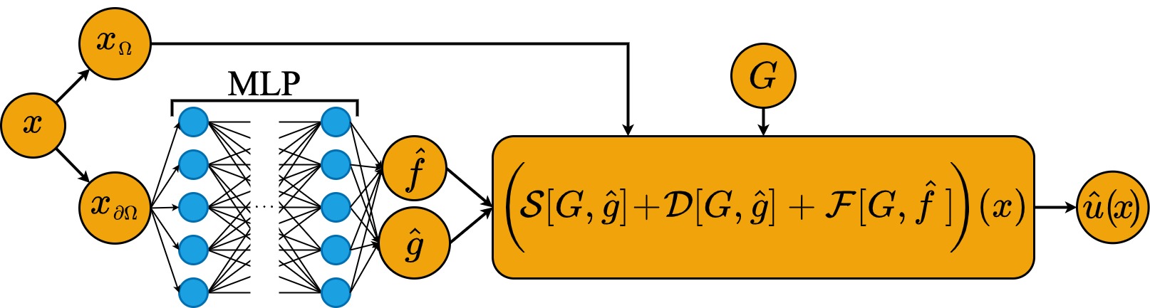
Figure 1: Visualisation of the PIBI-Net architecture.

In the implementation of PIBI-Net, we employ a multi-layer perceptron (MLP) to learn an approximation $\hat{g}$ of the boundary density function and, if present and unknown, the parameters for $\hat{f}$. The hat indicates the surrogate parameters and functions. The input variable $\bm{x}$ needs to be distinguished between points $\bm{x}_{\partial\Omega}$ on the boundary and points $\bm{x}_{\Omega}$ inside the domain. During training, $\bm{x}_{\Omega}$ contribute solely to the boundary integral representation (11), while the boundary points $\bm{x}_{\partial\Omega}$ serve as input to the MLP. The MLP is exchangeable with any suitable network, such as a fully connected neural network or a Siren-Net [Sitzmann et al. (2020)]. Automatic differentiation in common deep learning frameworks like PyTorch [Paszke et al. (2019)] and TensorFlow [Abadi et al. (2016)] enables the MLP to learn both the boundary density function $\hat{g}$ and its derivative.

Data measurements $u_{\text{data}}$ at $\bm{x}_{\text{data}}$ can be located either inside the domain $\Omega$ or on the boundary. Consequently, the only points we need to consider during the training phase within the domain are data measurements. The points $\bm{x}_{\partial\Omega}$ on the boundary, that serves as inputs of the MLP during training, have three different purposes: First, if present, as data measurements at $\bm{x}_{\text{data}}$ to ensure the data assimilation of the solution. Second, similar to PINNs, as collocation points $\bm{x}_{\text{coll}}$ to enforce the surrogate of the boundary density $\hat{g}$ at the boundary $\partial\Omega$. And lastly, as integral points $\bm{x}_{\text{int}}$ of the Monte Carlo integration to approximate the boundary integral representations (11).

In order to train PIBI-Net, the loss function $\mathcal{L}$ expressed by

$$\mathcal{L}:=\big{\|}\hat{u}(\bm{x}_{\text{data}})-u_{\text{data}}\big{\|}_{2}^{2}+\lambda\big{\|}\hat{u}(\bm{x}_{\text{coll}})-\hat{f}(\bm{x}_{\text{coll}})\big{\|}_{2}^{2},$$ (13)

is minimised via a gradient-based optimiser like Adam [Kingma and Ba (2014)]. Here, $\hat{u}$ denotes the surrogate of the PDE solution $u(\bm{x})$ and $\lambda\in\mathbb{R}$ serves as a weighting parameter.

We want to point out that the source term $\hat{f}$ needs to be learnt as an additional parameter only if it is not precisely known. In many real-world applications, we typically have prior knowledge about the number $M$ of point sources and a general understanding of their approximate locations. However, in an inverse problem setting where the point sources are unknown, we only need to learn the magnitudes $c_{0_{1}},\ldots,c_{0_{M}}$ and, if necessary, their exact locations $\bm{y}_{0_{1}},\ldots,\bm{y}_{0_{M}}$, as stated in (12). However, after the training procedure of PIBI-Net, we still need to compute the boundary integral representation defined by (11) at each point $\bm{x}$ for which we wish to evaluate the PIBI-Net solution. Despite the additional computation of the boundary integral representation, the use of Monte Carlo integration nevertheless ensures fast evaluation.

3 Experiments and Results

We showcase the power of the PIBI-Net in comparison to PINNs. For this purpose, we present three experiments to cover both, homogeneous and non-homogeneous PDEs with unknown point source terms. In subsection 3.1 we demonstrate PIBI-Net on a toy example with synthetic data distributed throughout the entire computational domain for the Laplace equation. In this experiment, we show that PIBI-Nets work as well accurately to assimilate data as PINNs. However, PIBI-Nets show even better results compared to PINNs when data is only available in some areas of the computational domain, which we present in subsection 3.2. To cover the relevance of solving data-driven non-homogeneous PDEs with point sources, we apply PIBI-Net to real-world measurements for groundwater flows in subsection 3.3.

3.1 Laplace Equation with a distributed data set over the entire domain

We compare PIBI-Net with PINNs for the two-dimensional Laplace equation based on $80$ data measurements, and use the finite difference method as a ground truth reference on an equidistant mesh with mesh size $\Delta x=0.2$. We constructed the data set by $80$ randomly sampled measurements from the solution obtained through the finite difference method on Laplace equation $\Delta u(\bm{x})=0$ in $\Omega:=(-1,1)^{2}$ with the Dirichlet boundary conditions given as

$$\left.\begin{aligned} u(x_{1}=-1,x_{2})&=\sin\left(\tfrac{3}{2\pi}\;x_{2}+\tfrac{\pi}{2}\right)\\ u(x_{1}=1,x_{2})&=\tfrac{1}{2}(x_{2}+1)\\ u(x_{1},x_{2}=-1)&=\begin{cases}\begin{aligned} 1-x_{1},\;\;\;\,&x_{1}\geq 0\\[2.15277pt] x_{1}+1,\;\;\;\;&x_{1}<0\end{aligned}\end{cases}\\ u(x_{1},x_{2}=1)&=\begin{cases}\begin{aligned} 1,\;\;\;\,&x_{1}\geq 0\\[2.15277pt] 1-|x_{1}|,\;\;\;\;&x_{1}<0,\end{aligned}\end{cases}\end{aligned}\right\}$$ (14)

whereas $\bm{x}=(x_{1},x_{2})$ denotes a point in the closure $\bar{\Omega}:=[-1,1]\times[-1,1]$ as a subset of $\mathbb{R}^{2}$. As in many real-world applications, we have only given data measurements and treat therefore the boundary conditions as unknowns.

PIBI-Net

Ground Truth

PINN

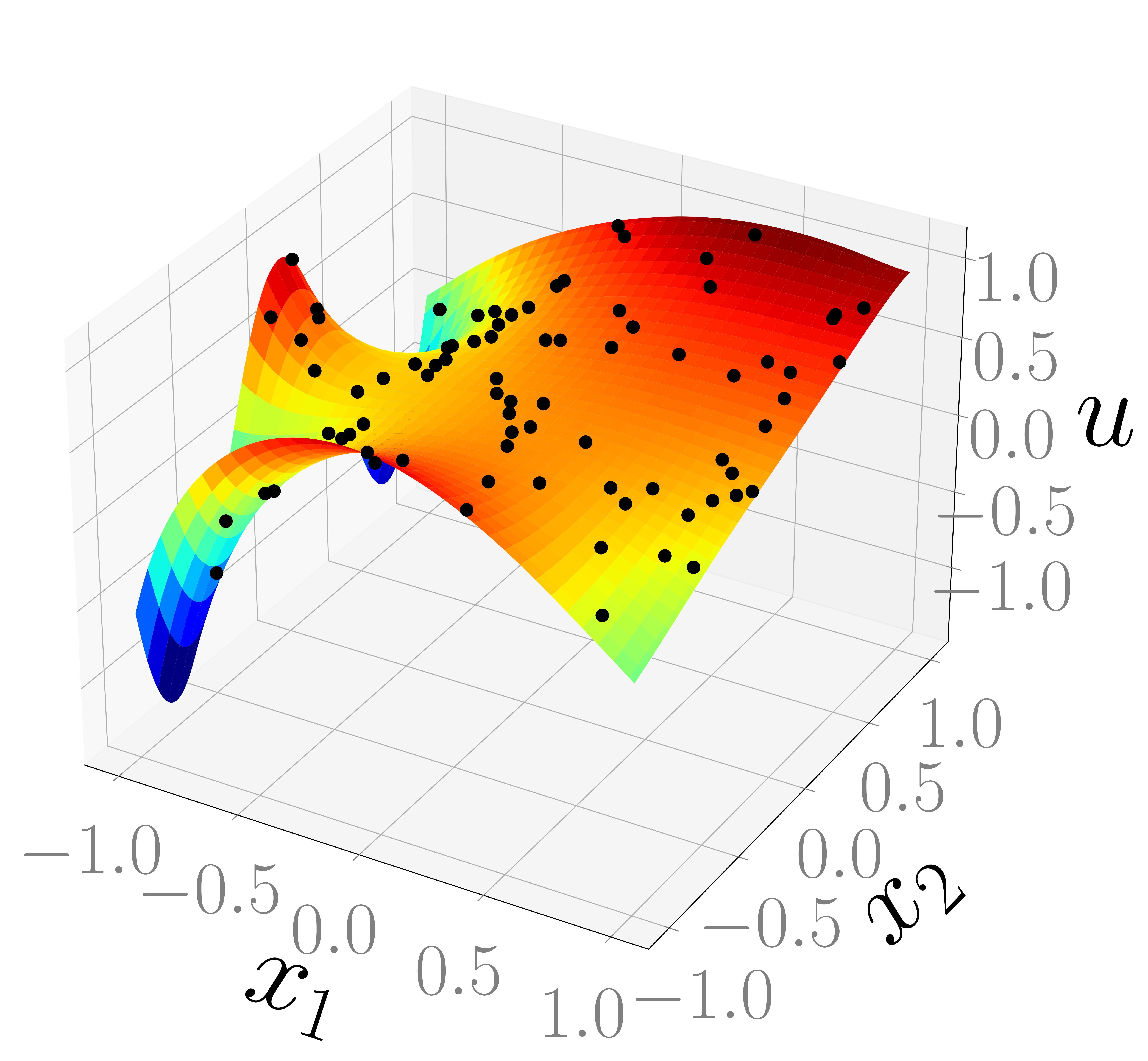
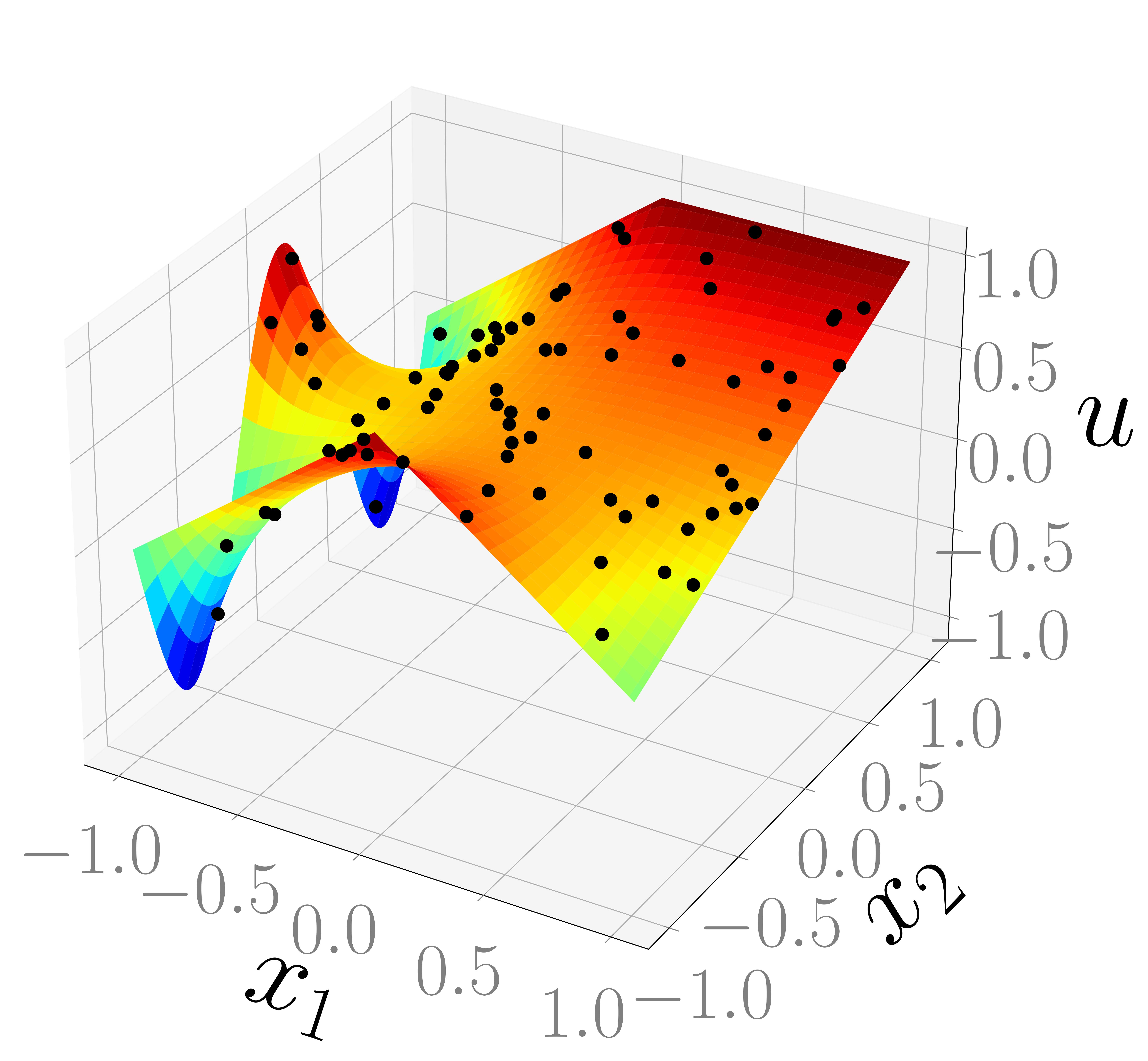
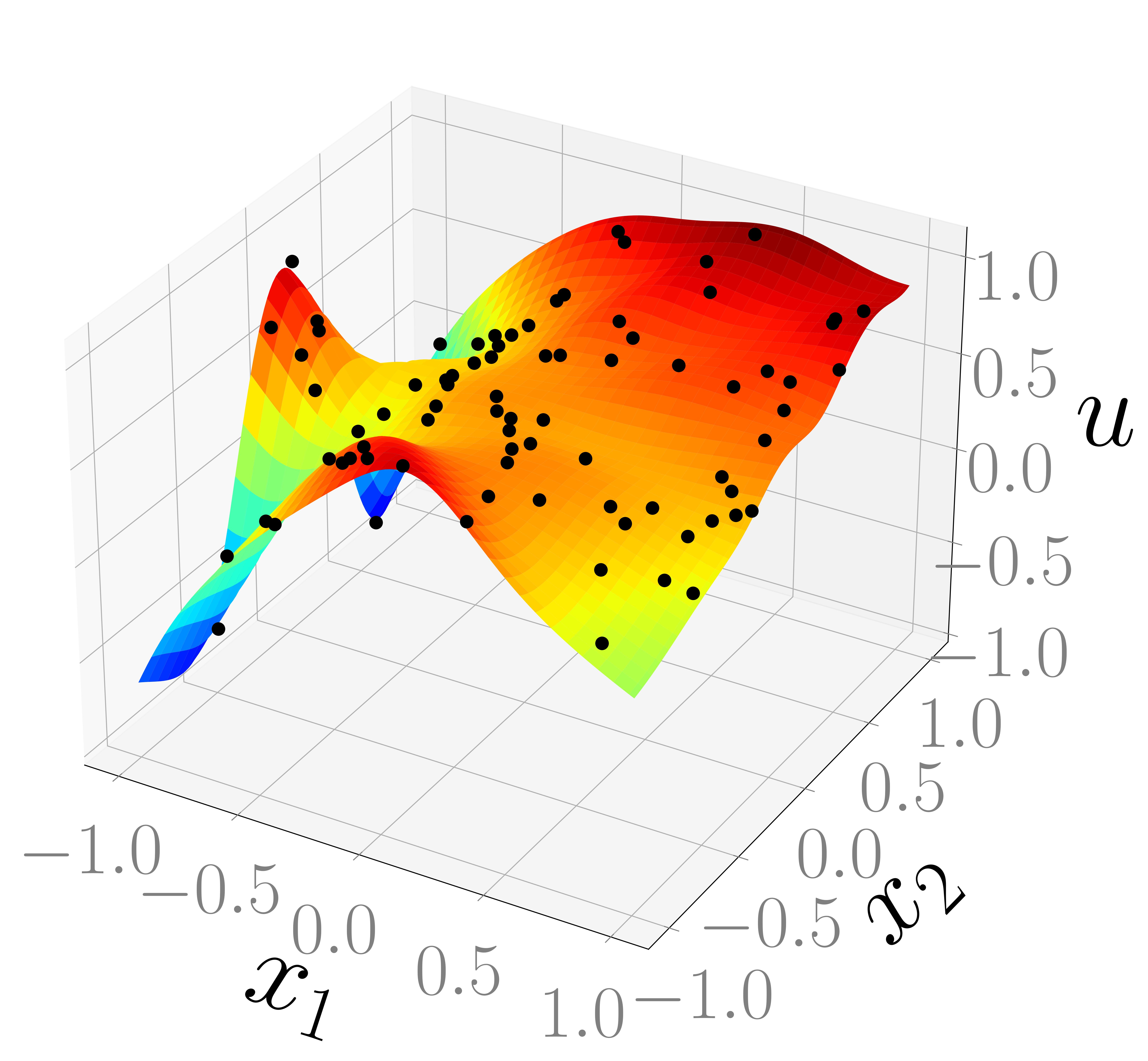
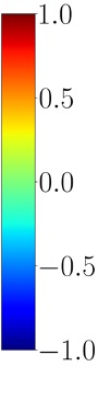
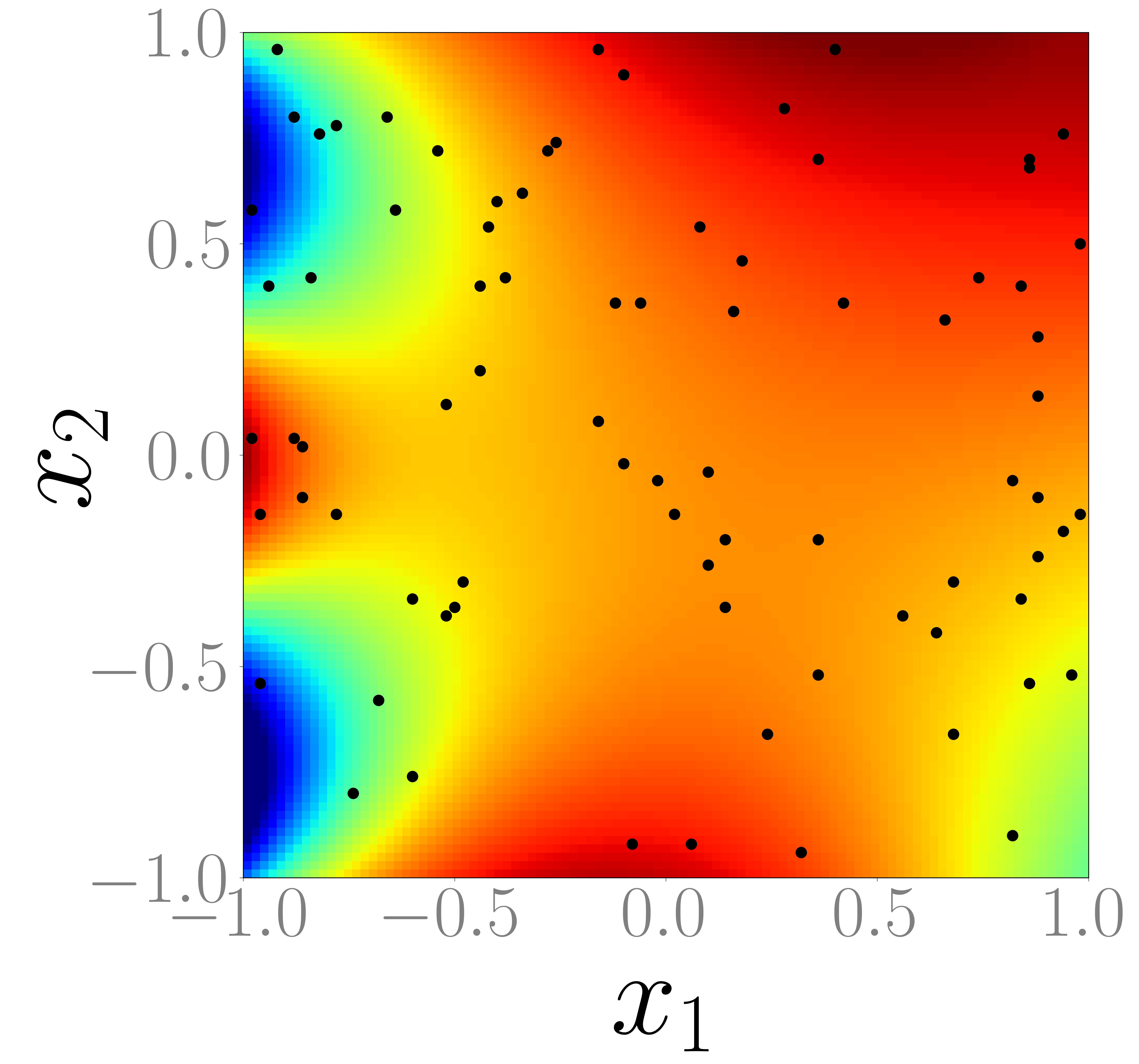
(Top View)

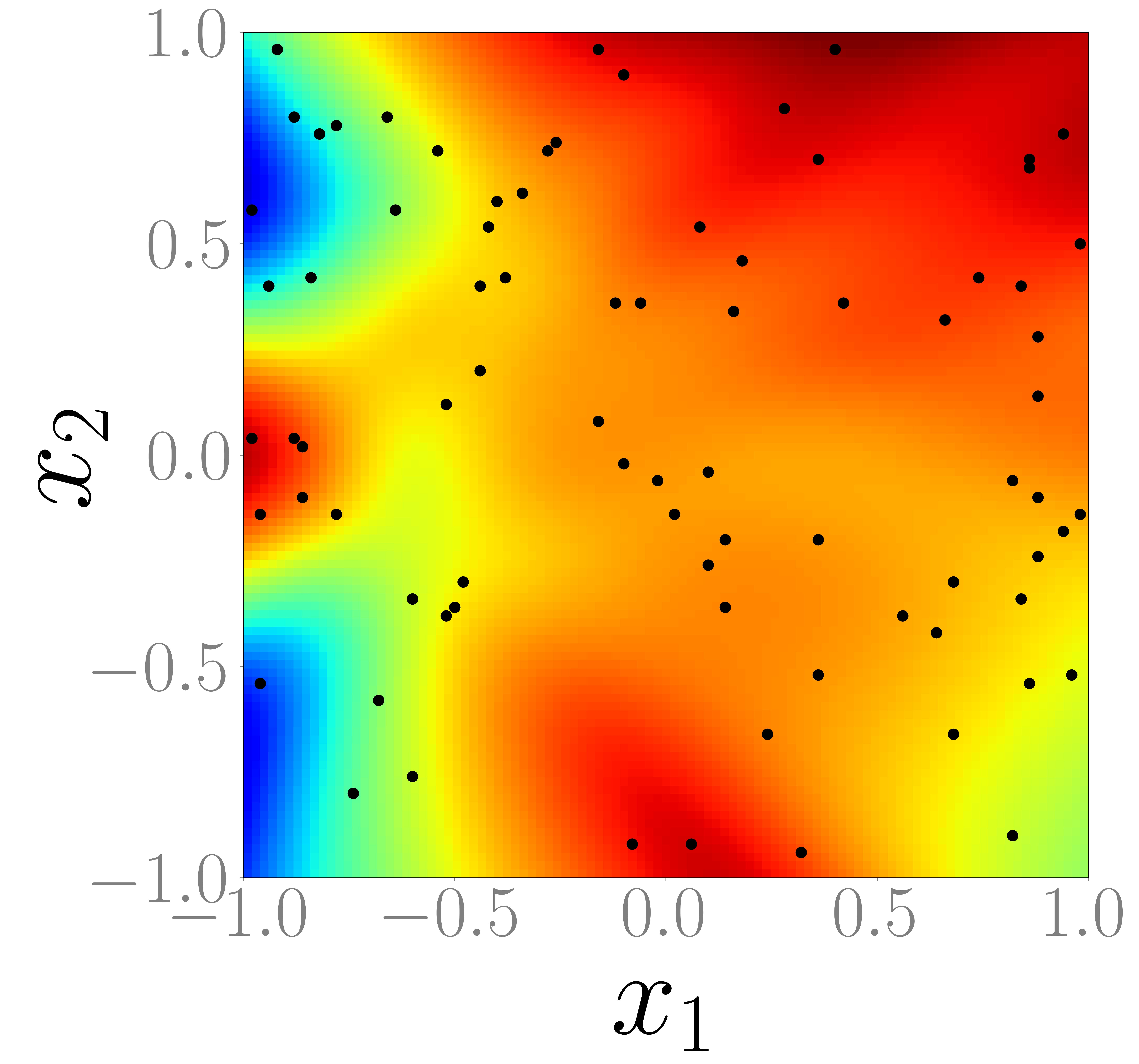
(Pixel-wise absolute error)

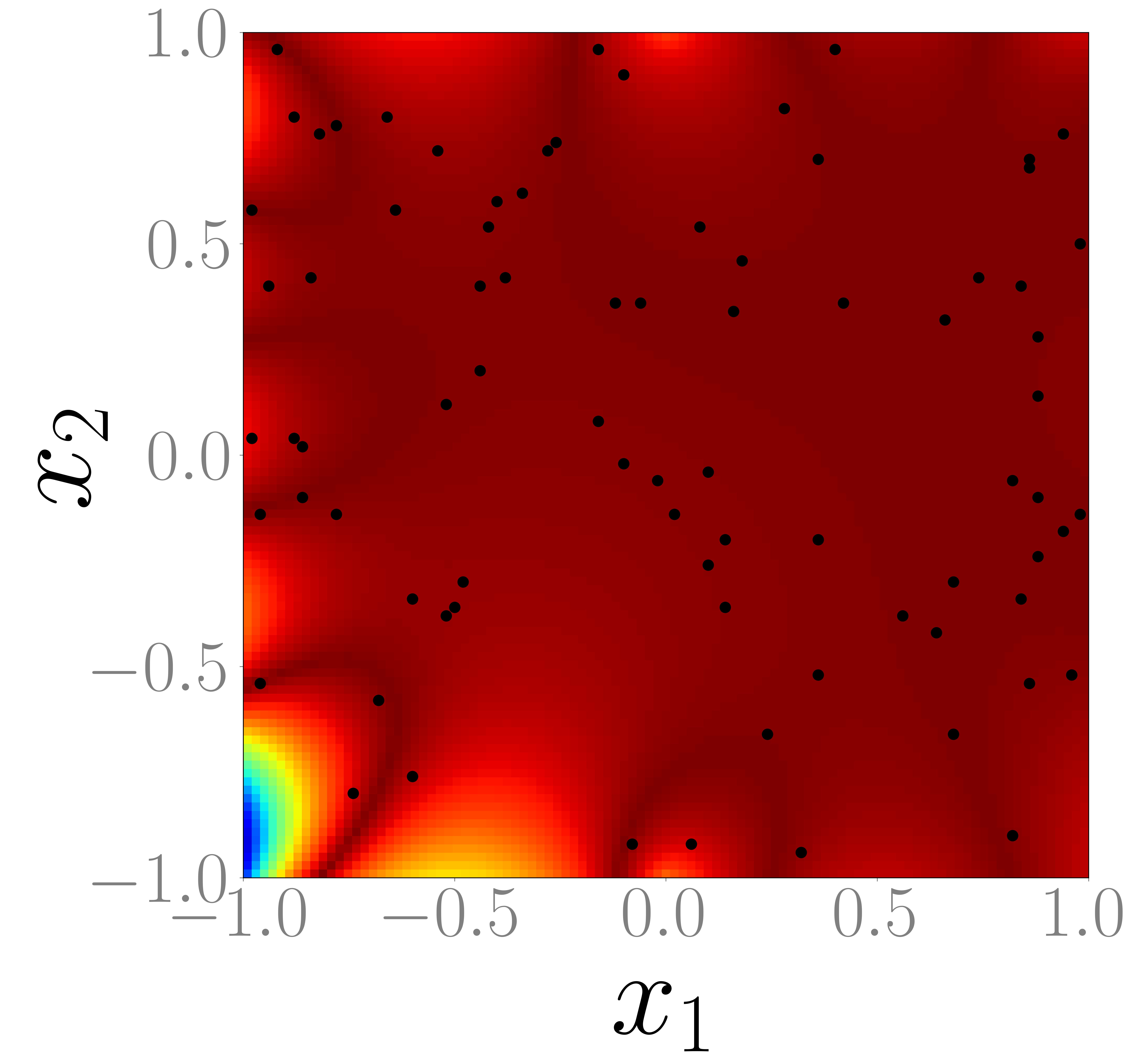
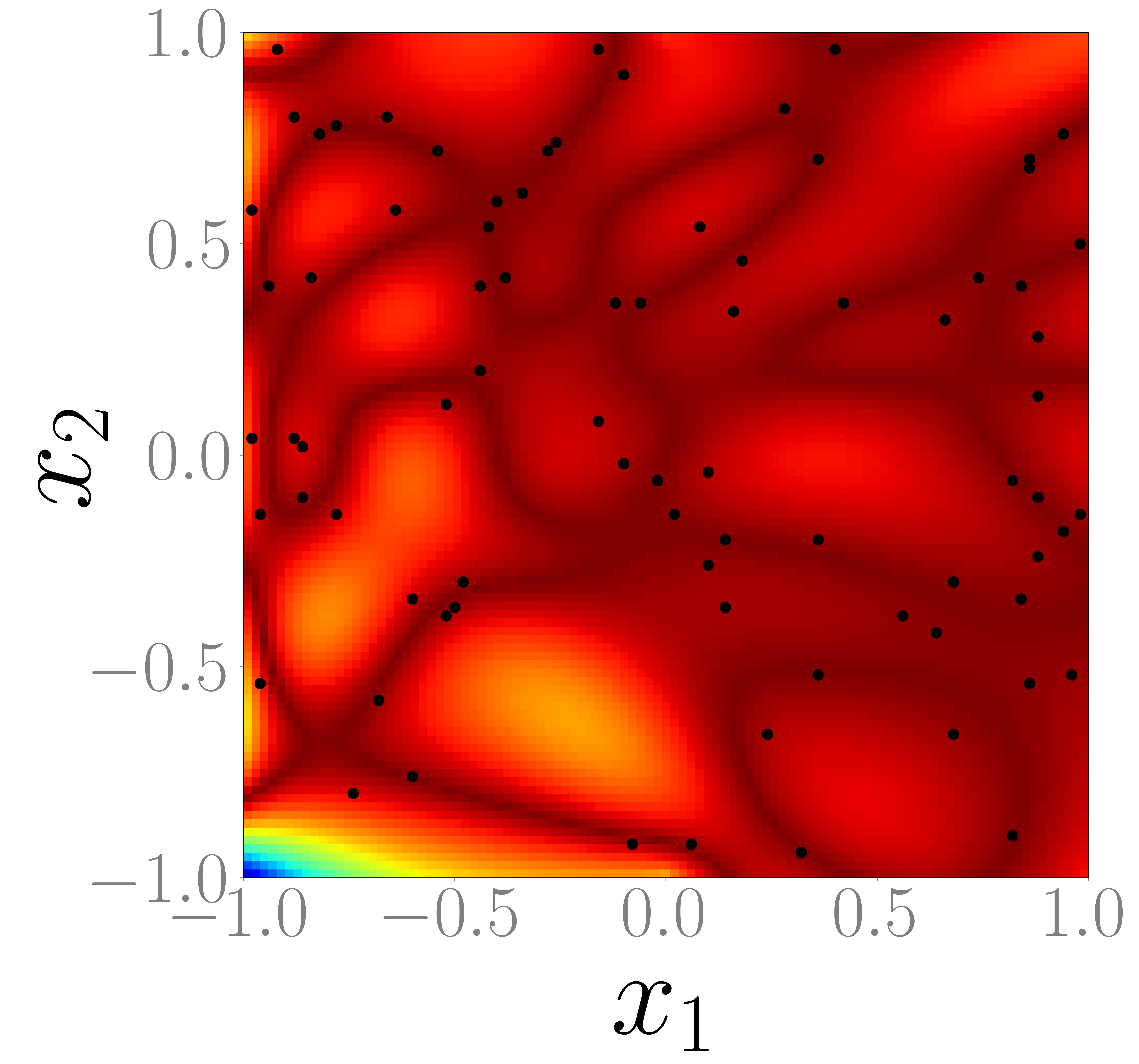
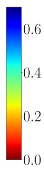
Figure 2: Visualisation of the 2D Toy example for solving the Laplace equation using $80$ measurements randomly sampled over entire domain $\Omega$ from the ground truth solution based on (14). The data measurements are indicated as black dots. We compare PIBI-Net listed in the first column to PINNs in the last column. We display the three-dimensional representations (top row), the projection to the $x_{1}=x_{2}$ plane (middle row) and the pixel-wise absolute errors with respect to the ground truth (bottom row).

We obtained the results in Figure 2 by training PIBI-Net with $1000$ boundary points, which we divided equally into $500$ collocation and $500$ integration points. To provide a fair comparison, we trained the PINN with $1000$ collocations points as well, but in this case sampled over the entire domain. For the PINN, we defined the loss function as $\|\hat{u}_{\text{PINN}}(\bm{x}_{\text{data}})-u_{\text{data}}\|_{2}^{2}+\lambda_{\text{physics}}\|\hat{u}_{\text{PINN}}(\bm{x}_{\text{coll}})\|_{2}^{2}$, where $\hat{u}_{\text{PINN}}$ represents the solution obtained by the network and $\lambda_{\text{physics}}$ a weighting factor to balance both loss terms.

In many real-world applications, the actual computational boundary can often be chosen freely. In this experiment, one option would therefore be to take the edges of the box $\Omega$. However, we found that a circle around the origin with a radius of $1.5$ is a better choice, as it avoids singularities that would appear at the corners of $\Omega$. In this way, all data measurements lie within our chosen circle.

As MLP, we used in both approaches a fully connected neural network with three hidden layers consisting $512$ neurons each. In PIBI-Net we achieved the best results with Exponential Linear Unit (ELU) from Clevert et al. (2015), and for the PINN approach with hyperbolic tangent activation functions. We trained the network with Adam [Kingma and Ba (2014)] as a gradient-based optimiser until it converged. For the loss function we used the mean squared error metric. To analyse and compare the accuracy of the two methods, we subtracted pixel-wise the ground truth from the PIBI-Net respectively the PINN solution. The resulting pixel-wise absolute error plot is shown in the last row of Figure 2. Comparing the mean and standard deviation from the pixel-wise absolute error of the two methods over five trained runs, we found that PIBI-Net with a mean error of $0.0348\pm 0.00453$ is comparable in accuracy to PINNs with a mean error of $0.04455\pm 0.01138$. Exemplified one of the trained runs in Figure 2, we achieved a maximum pixel-wise deviation with PIBI-Net as $0.6397$, and with the PINN as $0.6443$.

3.2 Laplace Equation with a clustered data set close to the domain boundary

In this section we use the same Laplace equation (14) as in subsection 3.1 as ground truth solution, but we only take $30$ measurement points that are in the area close to the boundary. Thereof, we do not have data measurements in the center area of the domain. Figure 3 presents the results we obtained by the PIBI-Net as well as the PINN approach. We used the same network setup as previously.

PIBI-Net

Ground Truth

PINN

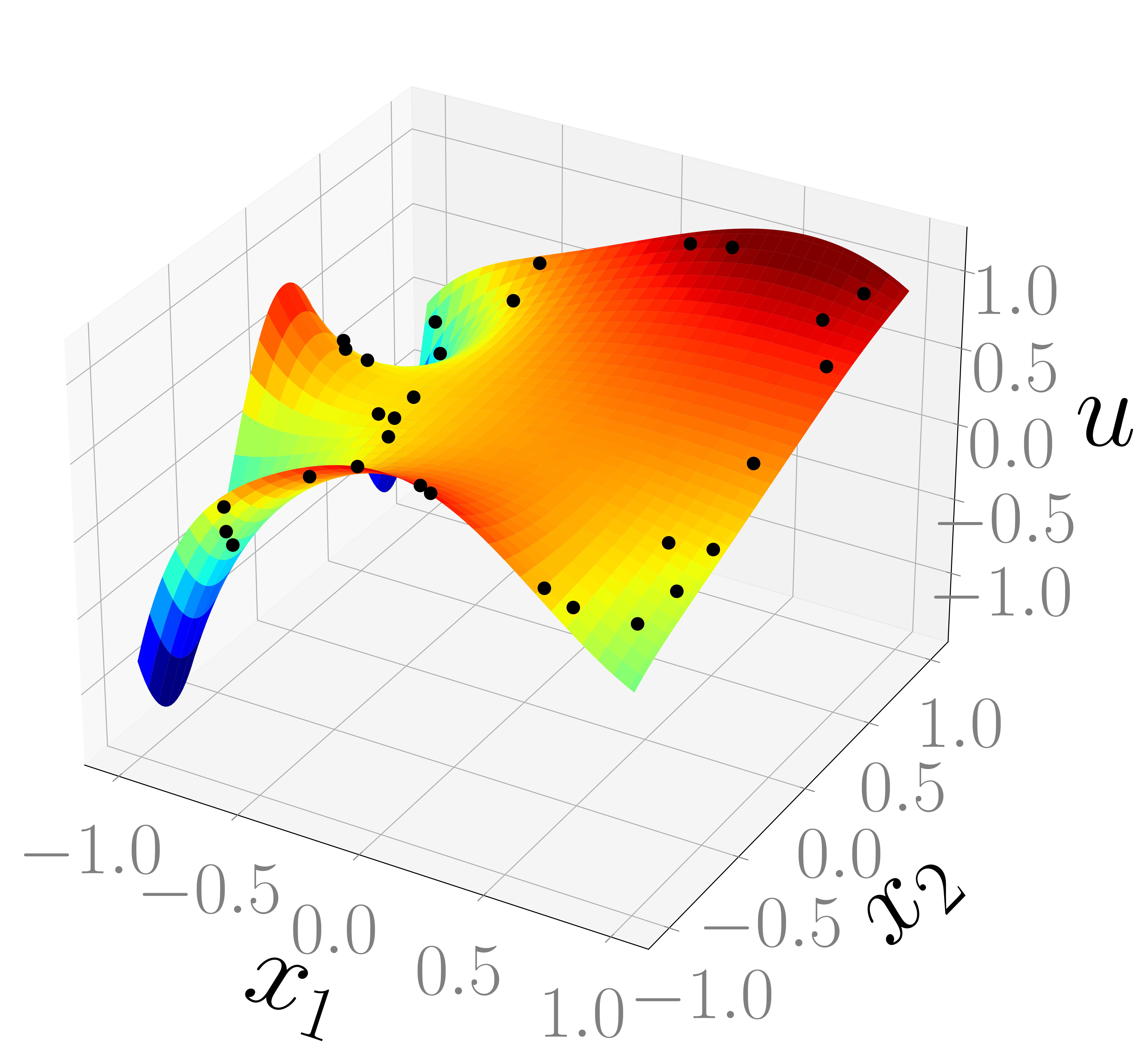
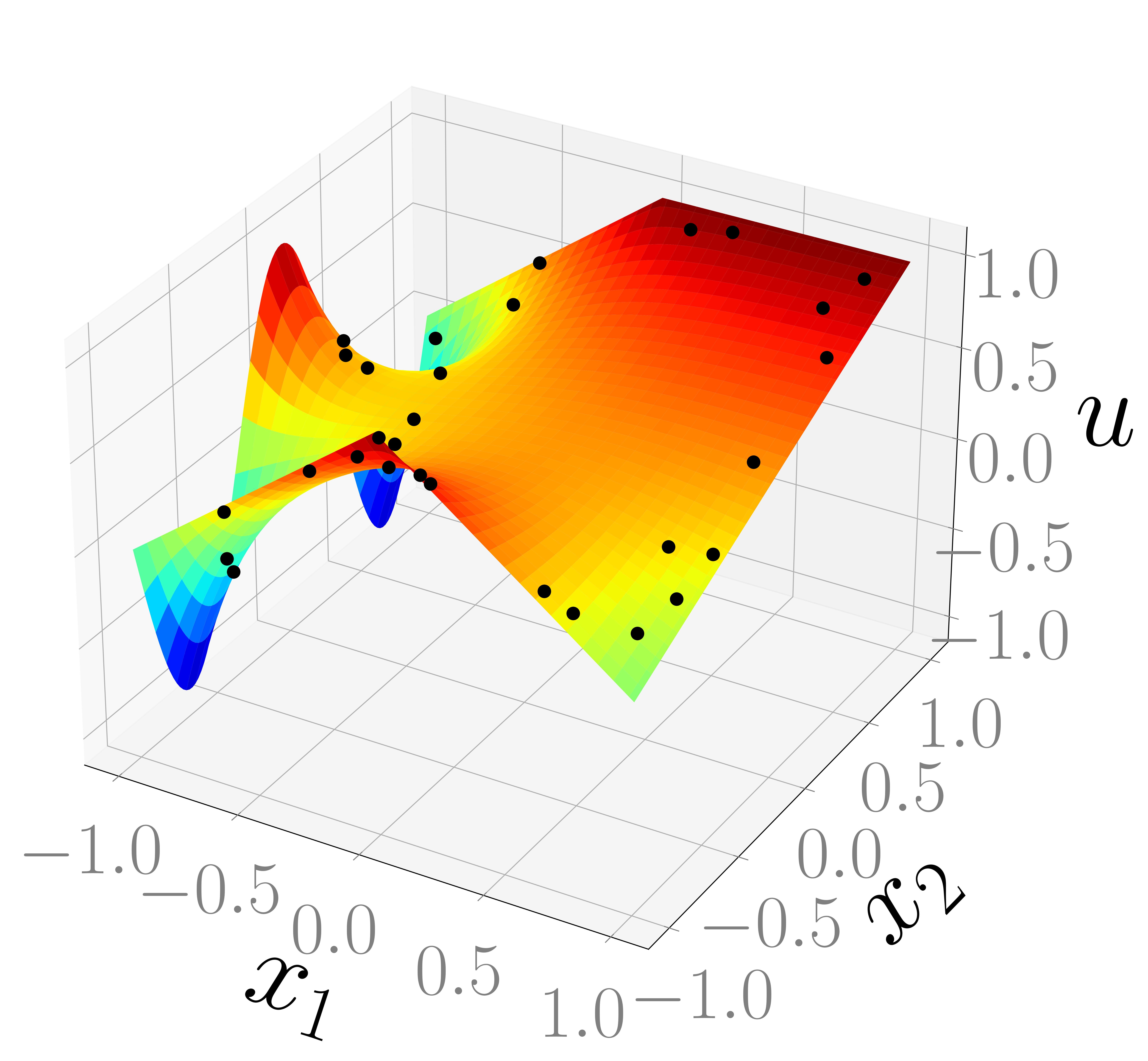
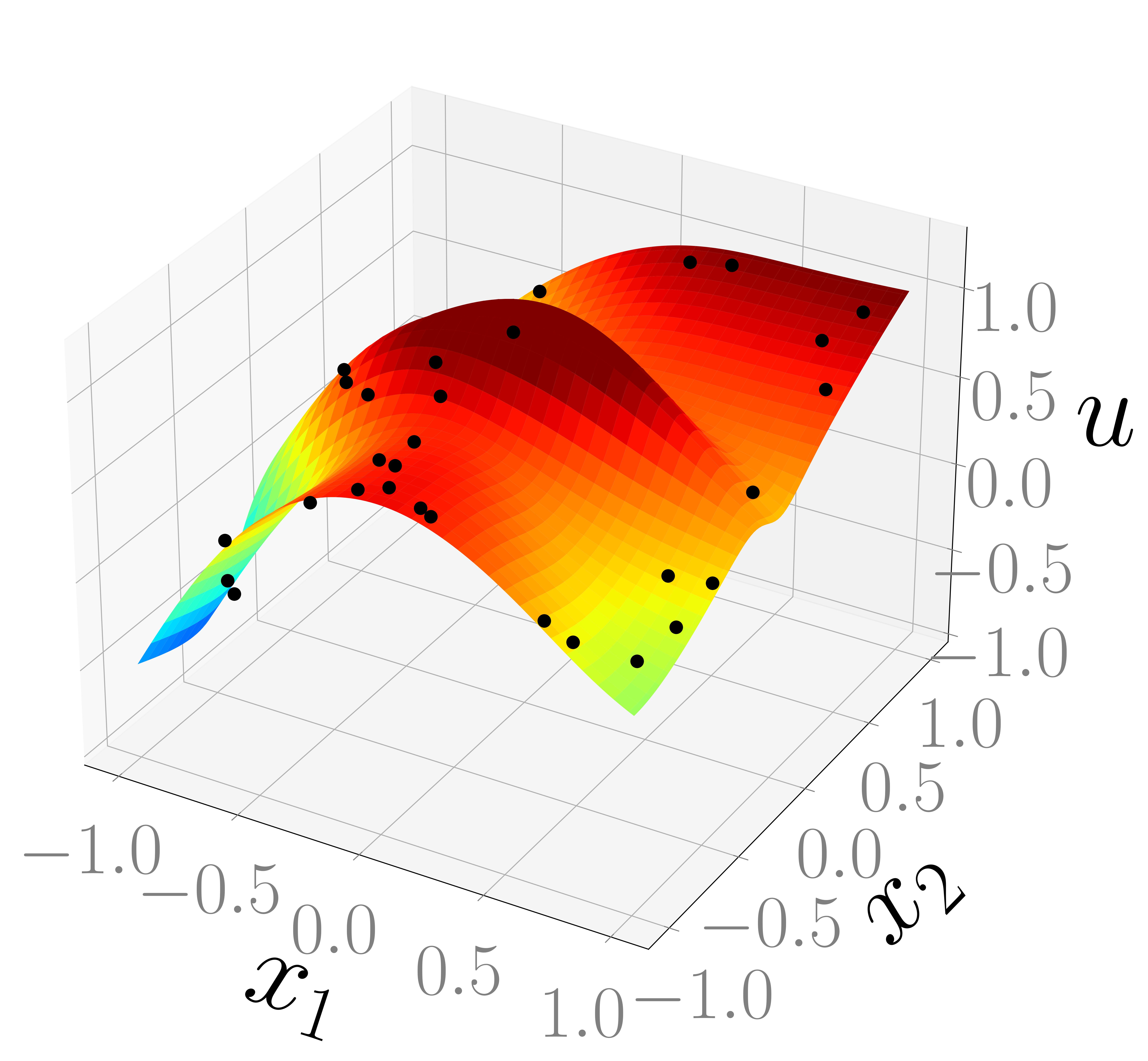
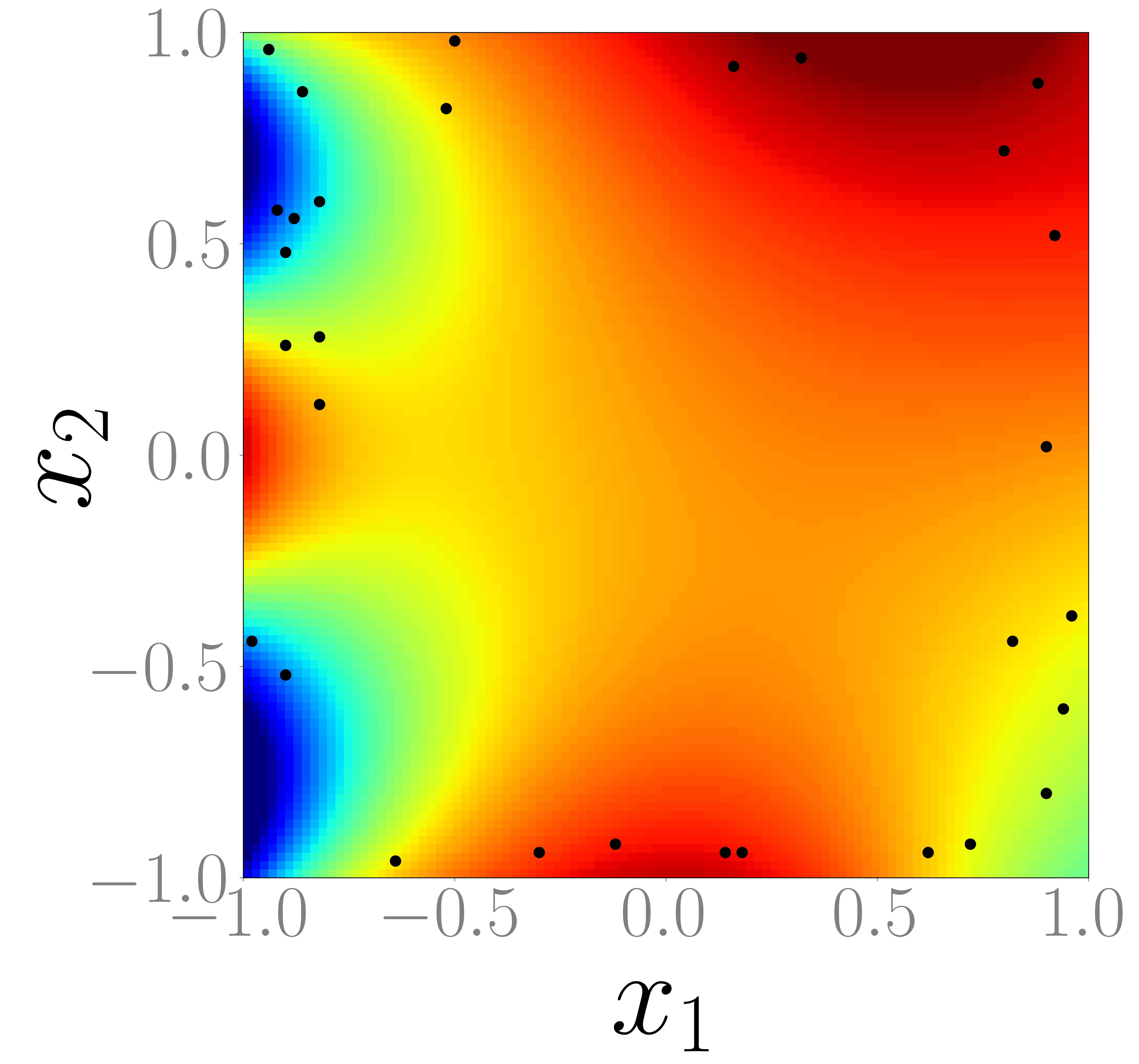
(Top View)

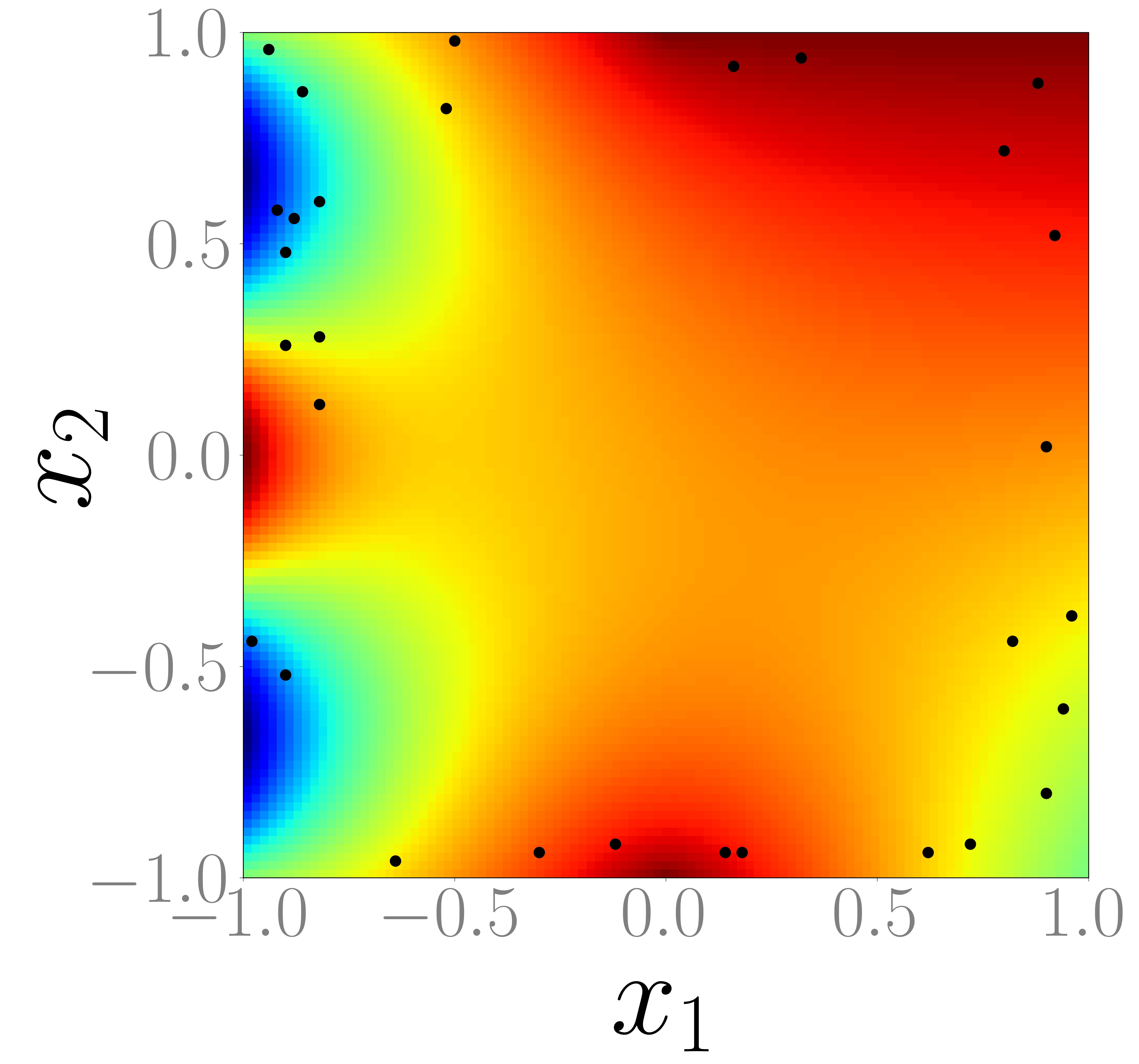
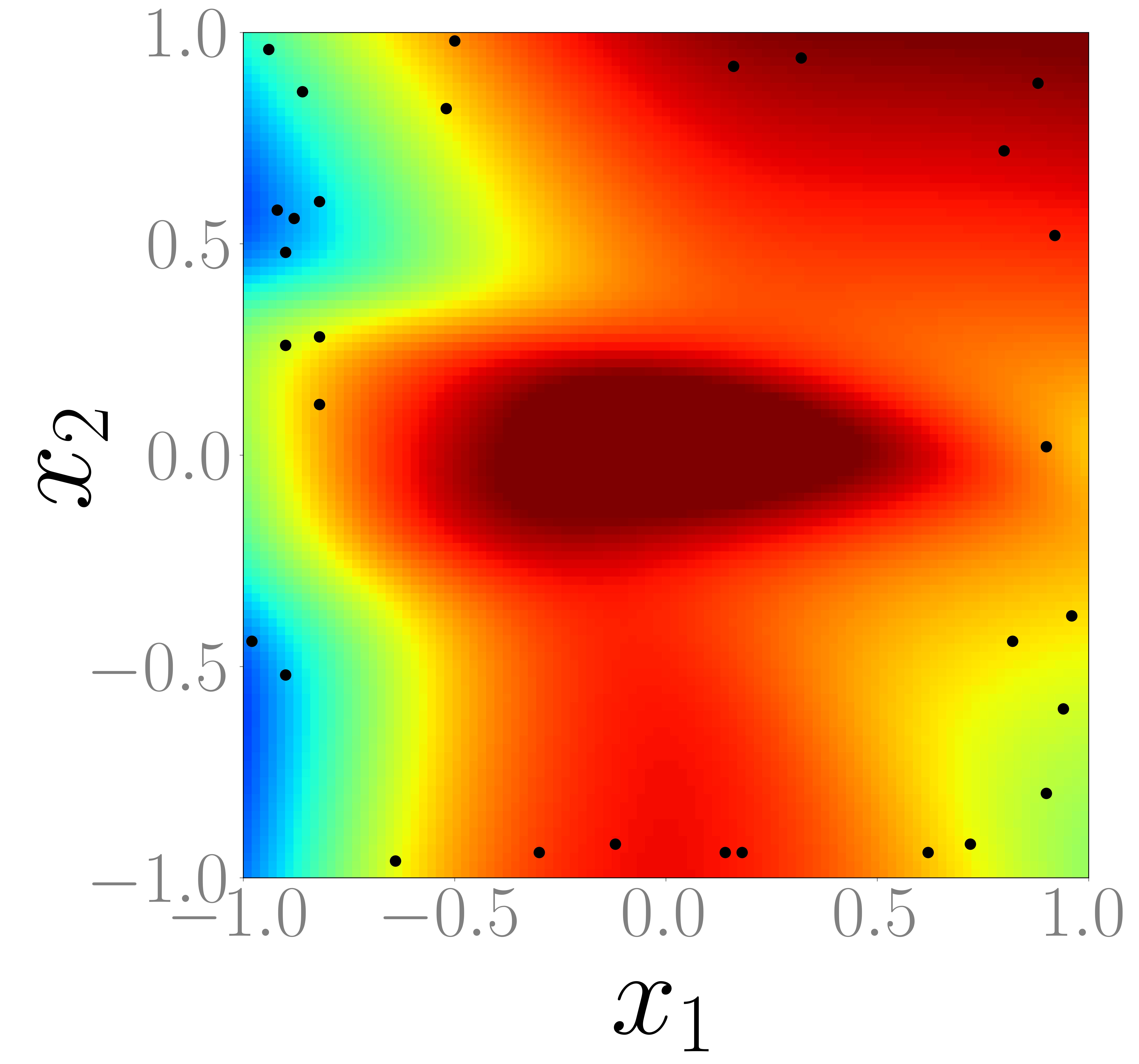
(Pixel-wise absolute error)

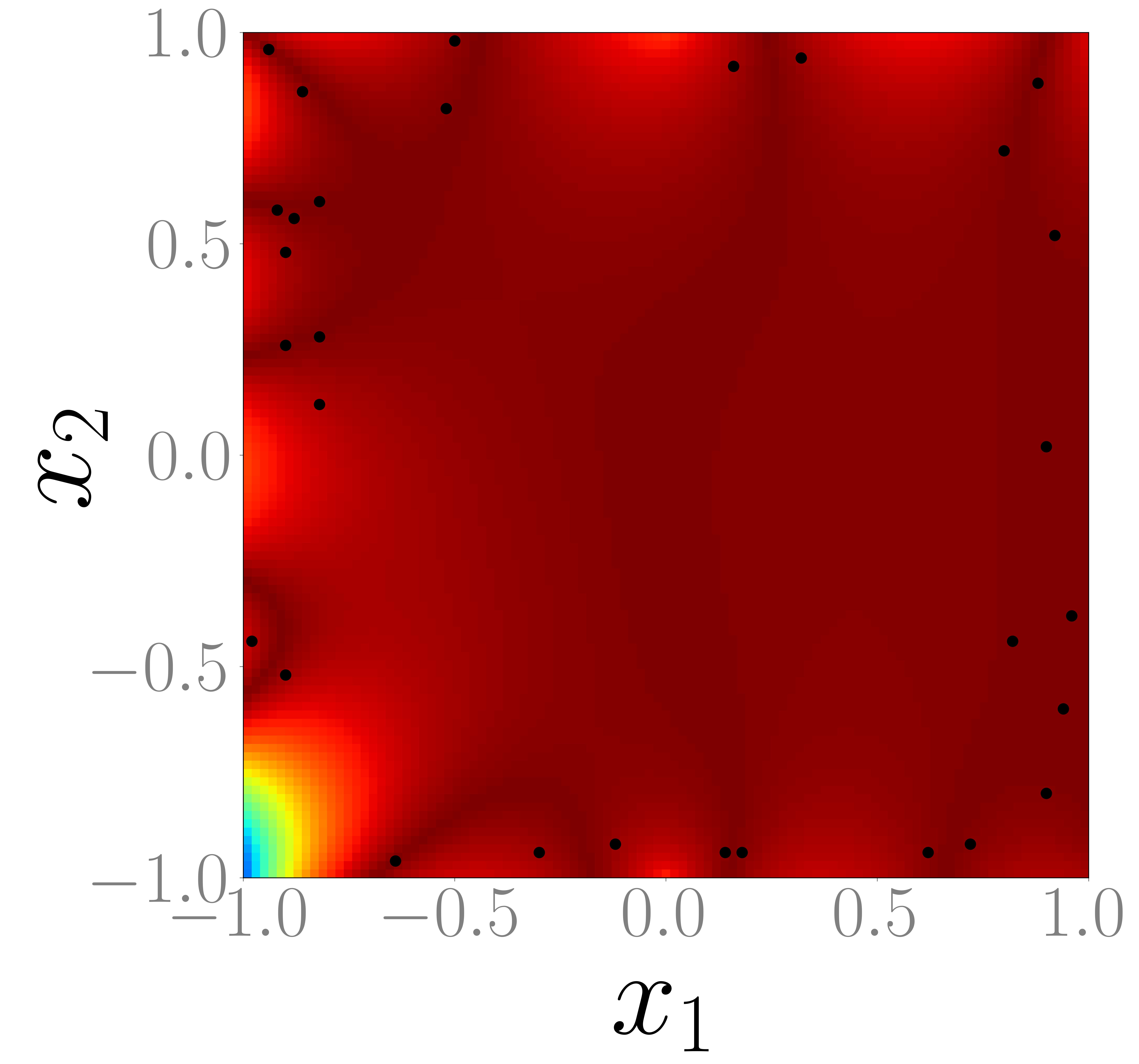
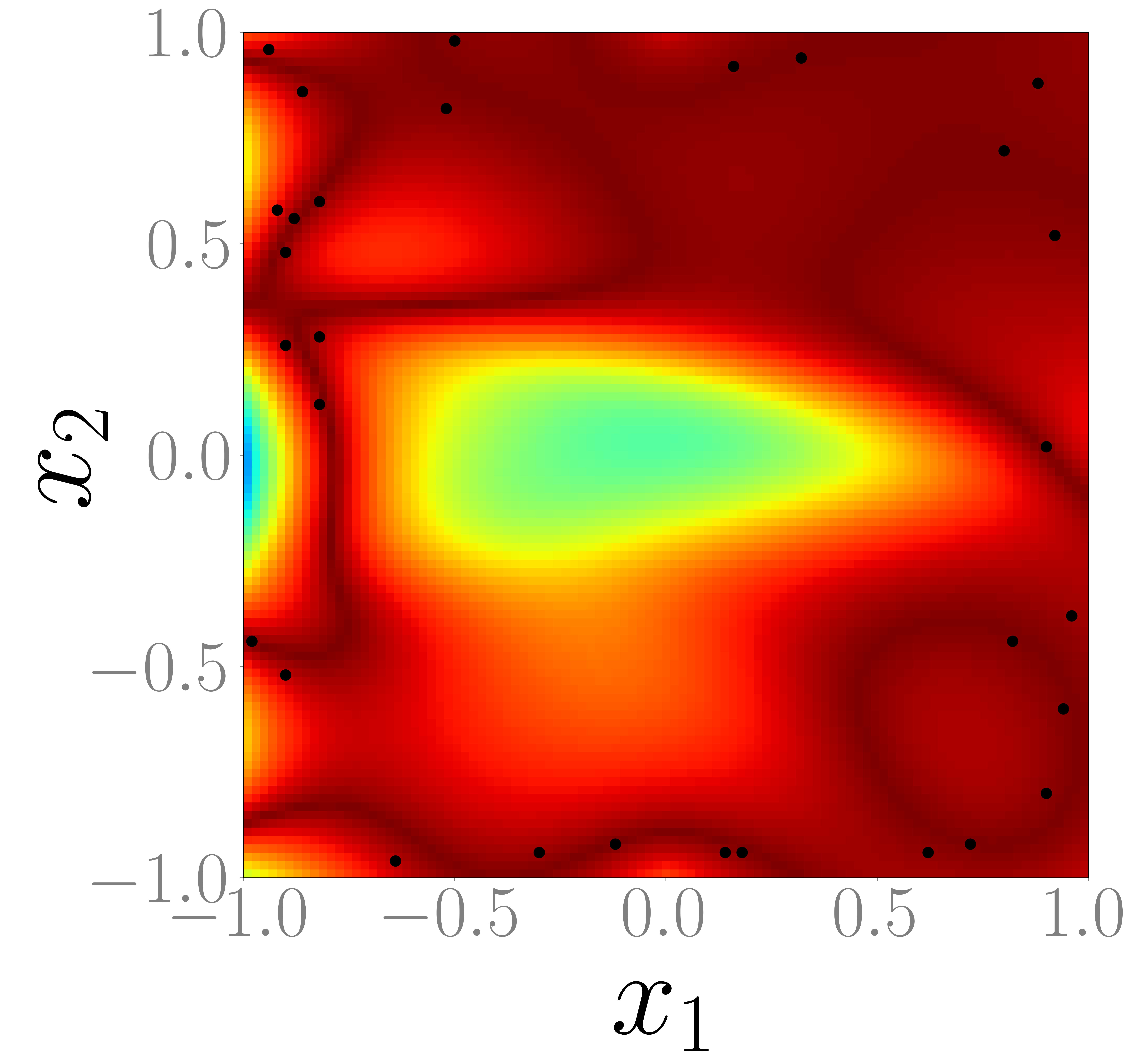
Figure 3: Visualisation of the 2D Toy example for solving the Laplace equation (14) using $30$ measurements randomly sampled in the area close to the boundary $\partial\Omega$.

As before in the previous toy example in subsection 3.1, we calculated the mean as well as the standard deviation of both approaches over five trained runs. For each training phase, we sampled new data measurements. PIBI-Net achieved an accuracy with a mean error of $0.0269\pm 0.00028$, while PINNs had a mean error of $0.1458\pm 0.00269$. Figure 3 shows one of the trained runs.

3.3 Ground water-level measurements in Memphis aquifer in Steady-state

Steady-state flow of groundwater in a homogeneous aquifer can be described through the Laplace equation. However, in real-world scenarios it is challenging to find areas where this equation is fulfilled owing to the presence of pump wells in many places. In order to handle pump wells correctly, we need to include additional points source terms, which leads to the Poisson equation (2). Groundwater level altitudes becomes therefore important for studying historical water-level changes.

In our real-world experiment, we simulated the altitudes of the potentiometric surface of water for the Memphis area, Tennessee US, in fall $2000$ based on $64$ well measurements. The dataset is based on the water-level altitude measurements presented in Kingsbury (2018).

We used the same training settings as in the previous toy examples from subsection 3.1 but with ReLU activation functions.

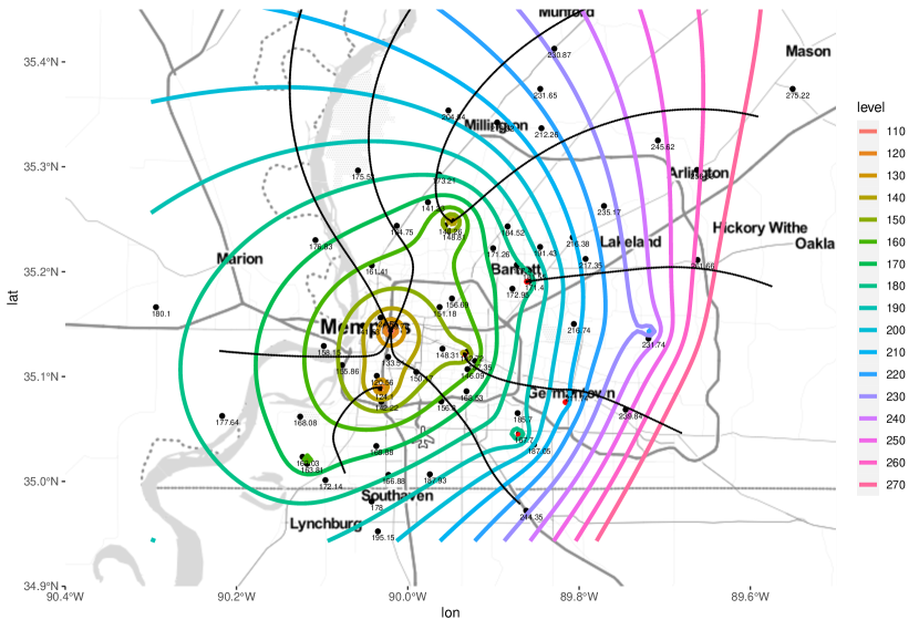
Figure 4: Visualisation of the water head contour lines based on the well measurements indicated as black dots. The black lines indicate the streamlines of the groundwater flows. The first column shows the results with PIBI-Net in contrast to the PINN in the second column. For these calculations, all data measurements were used. We add the magnitude and the location of the pump wells as additional learning parameters to the approaches.

We added additional learning parameters for the pump wells as sink terms to the experiments for groundwater level altitudes shown in Figure 4, as they are unknown. In particular, with the assumption that there is a pump well in each well field presented in Kingsbury (2018), we learned $2\times 8$ additional parameters with the MLP, one for the location and one for the magnitude of each pump well. We initialised the locations with one of the wells inside. We used the conjugated gradient method to calculate the streamlines and indicate the groundwater flows in Figure 4.

4 Discussion

We compared PIBI-Net to PINNs for the Laplace equation in sections 3.1 and 3.2 and showcased the performance of PIBI-Net for real-world observations in subsection 3.3. We have shown that PIBI-Net achieves at least comparable results in terms of accuracy to PINNs. However, we found some advantages as well as limitations.

• We have shown in Figure 3 that PIBI-Net outperforms PINNs in settings, where data is only available in areas close to the boundary. This might be relevant in real-world settings with sparse data sets.

• Since PIBI-Net only requires first-order derivatives, it enables us to use a broader range of MLP models with suitable activation functions.

• Adjusting the lambda hyperparameter in PIBI-Net is still needed to balance between the data and collocation loss terms. This can be challenging and time-consuming. However, this adjustment is also required in the PINN approach.

• As in other data-driven approaches, the solution of PIBI-Net relies strongly on the quality of the observations. If the observations do not cover the important regions for the dynamics, the problem might be ill-posed. Therefore, data-driven approaches cannot compete with solutions that contain more information through boundary conditions. Consequently, neither the PIBI-Net nor the PINN approach can cover, for example, the lower left corner because of missing observations.

• Since data points can lie on the boundary, and both collocation and integral points are located on the boundary $\partial\Omega$ as well, a careful selection is required to prevent singularities when they are too close to each other. Our experience has shown that a regular grid over the boundary shows the best results. We assigned every second point as an integral point and the rest as collocation points. By rotating the points slightly in each iteration, this approach can still add some level of randomness.

• As the integral calculation of PIBI-Net is based on the Monte Carlo integration, a reasonable amount of integration points is needed to obtain valid results. On one hand, too few integral points would lead to a wrong calculation of the integral. On the other hand, too many integral points could lead to singularities, as the distance between the collocation and integral points goes to zero. In our experiments, we found that the results with 1000 boundary points evenly divided into 500 collocation and 500 integral points give already good results.

• In our real-world experiment to simulate groundwater altitudes, we presented a setting where the reformulation of point sources given by equation (12) is useful and can be used in any physics-informed deep learning approach. However, in the case of non-homogeneous PDEs with non-point sources, we would lose PIBI-Net’s advantage of the dimension reduction by one, as the integral needs to be solved over the entire domain.

5 Conclusion

We have shown that PIBI-Net as a data-driven deep learning approach delivers comparable results in accuracy to a PINN, while requiring only collocation points at the boundary. Even more, PIBI-Net outperforms PINNs in settings where data is clustered in regions close to the boundary, but missing in the middle area of the computational domain. This brings an enormous advantage in many problem settings, as most data-driven real-world applications are in three or four dimensions. PIBI-Net can be used for all dynamical systems that are based on a linear PDE with constant coefficients.

In the two-dimensional toy example, we have shown that the mean absolute error of the PIBI-Net solution falls within the same error range as from the PINN approach. Additionally, in the real-world steady-state groundwater application, we demonstrated that PIBI-Net can also deal with inverse problems by learning the location and magnitude of point sources. For non-point sources, however, an integral over the entire domain must still be solved. With Monte Carlo integration, one would lose the dimension reduction advantage of PIBI-Net. Therefore, further research needs to be done in this direction.

Data availability

Data from Kingsbury (2018) was used for the ground water simulation. The implementations that generated the presented results are available on our Github repository at the following link: https://github.com/MonikaNagy-Huber/PIBI-Net.git.

References

- Abadi et al. (2016) Abadi, M., Barham, P., Chen, J., Chen, Z., Davis, A., Dean, J., Devin, M., Ghemawat, S., Irving, G., Isard, M., et al., 2016. Tensorflow: a system for large-scale machine learning., in: Osdi, Savannah, GA, USA. pp. 265–283. https://dl.acm.org/doi/10.5555/3026877.3026899.
- Anderson et al. (2013) Anderson, J.D., Degrez, G., Dick, E., Grundmann, R., 2013. Computational fluid dynamics: an introduction. Springer Science & Business Media. https://doi.org/10.1007/978-3-540-85056-4.
- Arcucci et al. (2021) Arcucci, R., Zhu, J., Hu, S., Guo, Y.K., 2021. Deep data assimilation: integrating deep learning with data assimilation. Applied Sciences 11, 1114. https://doi.org/10.3390/app11031114.
- Buizza et al. (2022) Buizza, C., Casas, C.Q., Nadler, P., Mack, J., Marrone, S., Titus, Z., Le Cornec, C., Heylen, E., Dur, T., Ruiz, L.B., et al., 2022. Data learning: integrating data assimilation and machine learning. Journal of Computational Science 58, 101525. https://doi.org/10.1016/j.jocs.2021.101525.
- Clevert et al. (2015) Clevert, D.A., Unterthiner, T., Hochreiter, S., 2015. Fast and accurate deep network learning by exponential linear units (elus). arXiv preprint arXiv:1511.07289 .
- Cuomo et al. (2022) Cuomo, S., Di Cola, V.S., Giampaolo, F., Rozza, G., Raissi, M., Piccialli, F., 2022. Scientific machine learning through physics–informed neural networks: where we are and what’s next. Journal of Scientific Computing 92, 88. https://doi.org/10.1007/s10915-022-01939-z.
- Ehrenpreis (1954) Ehrenpreis, L., 1954. Solution of some problems of division: Part i. division by a polynomial of derivation. American Journal of Mathematics 76, 883–903. https://doi.org/10.2307/2372662.
- Kesavan and Vasudevamurthy (1985) Kesavan, S., Vasudevamurthy, A., 1985. On some boundary element methods for the heat equation. Numerische Mathematik 46, 101–120. https://doi.org/10.1007/BF01400258.
- Khan and Lowther (2022) Khan, A., Lowther, D.A., 2022. Physics informed neural networks for electromagnetic analysis. IEEE Transactions on Magnetics 58, 1–4. http://dx.doi.org/10.1109/TMAG.2022.3161814.
- Kingma and Ba (2014) Kingma, D.P., Ba, J., 2014. Adam: A method for stochastic optimization. arXiv preprint arXiv:1412.6980 .
- Kingsbury (2018) Kingsbury, J.A., 2018. Altitude of the potentiometric surface, 2000–15, and historical water-level changes in the Memphis aquifer in the Memphis area, Tennessee. Technical Report. US Geological Survey. https://doi.org/10.3133/sim3415.
- Lin et al. (2023) Lin, G., Chen, F., Hu, P., Chen, X., Chen, J., Wang, J., Shi, Z., 2023. Bi-greennet: learning green’s functions by boundary integral network. Communications in Mathematics and Statistics 11, 103–129. https://doi.org/10.1007/s40304-023-00338-6.
- Malgrange (1956) Malgrange, B., 1956. Existence et approximation des solutions des équations aux dérivées partielles et des équations de convolution, in: Annales de l’institut Fourier, pp. 271–355. https://doi.org/10.5802/aif.65.
- Misljenovic (1982) Misljenovic, D.M., 1982. Boundary element method and wave equation. Applied Mathematical Modelling 6, 205–208. https://doi.org/10.1016/0307-904X(82)90012-9.
- Nussbaumer et al. (2021) Nussbaumer, R., Bauer, S., Benoit, L., Mariethoz, G., Liechti, F., Schmid, B., 2021. Quantifying year-round nocturnal bird migration with a fluid dynamics model. Journal of the Royal Society Interface 18, 20210194. https://doi.org/10.1098/rsif.2021.0194.
- Paszke et al. (2019) Paszke, A., Gross, S., Massa, F., Lerer, A., Bradbury, J., Chanan, G., Killeen, T., Lin, Z., Gimelshein, N., Antiga, L., et al., 2019. Pytorch: An imperative style, high-performance deep learning library. Advances in neural information processing systems 32. https://proceedings.neurips.cc/paper_files/paper/2019/file/bdbca288fee7f92f2bfa9f7012727740-Paper.pdf.
- Raissi et al. (2019) Raissi, M., Perdikaris, P., Karniadakis, G.E., 2019. Physics-informed neural networks: A deep learning framework for solving forward and inverse problems involving nonlinear partial differential equations. Journal of Computational physics 378, 686–707. https://doi.org/10.1016/j.jcp.2018.10.045.
- Sharma et al. (2023) Sharma, P., Chung, W.T., Akoush, B., Ihme, M., 2023. A review of physics-informed machine learning in fluid mechanics. Energies 16, 2343. https://doi.org/10.3390/en16052343.
- Sitzmann et al. (2020) Sitzmann, V., Martel, J., Bergman, A., Lindell, D., Wetzstein, G., 2020. Implicit neural representations with periodic activation functions, in: Larochelle, H., Ranzato, M., Hadsell, R., Balcan, M., Lin, H. (Eds.), Advances in Neural Information Processing Systems, Curran Associates, Inc.. pp. 7462–7473. https://proceedings.neurips.cc/paper_files/paper/2020/file/53c04118df112c13a8c34b38343b9c10-Paper.pdf.
- Steinbach (2007) Steinbach, O., 2007. Numerical approximation methods for elliptic boundary value problems: finite and boundary elements. Springer Science & Business Media. https://doi.org/10.1007/978-0-387-68805-3.
- Sun et al. (2023) Sun, J., Liu, Y., Wang, Y., Yao, Z., Zheng, X., 2023. Binn: A deep learning approach for computational mechanics problems based on boundary integral equations. Computer Methods in Applied Mechanics and Engineering 410, 116012. https://doi.org/10.1016/j.cma.2023.116012.
- Villalpando-Vizcaino et al. (2021) Villalpando-Vizcaino, R., Waldron, B., Larsen, D., Schoefernacker, S., 2021. Development of a numerical multi-layered groundwater model to simulate inter-aquifer water exchange in shelby county, tennessee. Water 13, 2583. https://doi.org/10.3390/w13182583.
- Wang et al. (2022) Wang, X., Zhu, S., Guo, Y., Han, P., Wang, Y., Wei, Z., Jin, X., 2022. Transflownet: A physics-constrained transformer framework for spatio-temporal super-resolution of flow simulations. Journal of Computational Science 65, 101906. https://doi.org/10.1016/j.jocs.2022.101906.
- Xun et al. (2013) Xun, X., Cao, J., Mallick, B., Maity, A., Carroll, R.J., 2013. Parameter estimation of partial differential equation models. Journal of the American Statistical Association 108, 1009–1020. https://doi.org/10.1080/01621459.2013.794730.
- Yang et al. (2021) Yang, L., Meng, X., Karniadakis, G.E., 2021. B-pinns: Bayesian physics-informed neural networks for forward and inverse pde problems with noisy data. Journal of Computational Physics 425, 109913. https://doi.org/10.1016/j.jcp.2020.109913.