Semantic relatedness in DBpedia:
A comparative and experimental assessment

Abstract

Evaluating semantic relatedness of Web resources is still an open challenge. This paper focuses on knowledge-based methods, which represent an alternative to corpus-based approaches, and rely in general on the availability of knowledge graphs. In particular, we have selected 10 methods from the existing literature, that have been organized according to adjacent resources, triple patterns, and triple weights based methods. They have been implemented and evaluated by using DBpedia as reference RDF knowledge graph. Since DBpedia is continuously evolving, the experimental results provided by these methods in the literature are not comparable. For this reason, in this work such methods have been experimented by running them all at once on the same DBpedia release and against 14 well-known golden datasets. On the basis of the correlation values with human judgment obtained according to the experimental results, weighting the RDF triples in combination with evaluating all the directed paths linking the compared resources is the best strategy in order to compute semantic relatedness in DBpedia.

Keywords Semantic relatedness  $\cdot$ knowledge graph  $\cdot$ Linked Data  $\cdot$ DBpedia.

1 Introduction

How much are two given words related? In general, the way of automatically computing a degree of relatedness between words falls into one of the following categories of methods [22]: corpus-based methods, which use large corpora of natural language texts, and exploit co-occurrences of words, as for instance [47]; knowledge-based methods, which rely on structured resources, as for instance [13]; and hybrid methods, which are a mix of the two, as for instance [38]. Corpus-based methods benefit from the huge availability of textual documents and the advancements in the field of natural language processing and, for this reason, they have been widely investigated in the literature for a long time. Knowledge-based methods mainly depend on the availability and the quality of a proper knowledge base, such as a knowledge graph or an ontology. These methods require words to be associated with resources in the knowledge base in order to shift from a pure linguistic dimension to a knowledge-based one. This paper focuses on knowledge-based methods.

Since the advent of the Semantic Web, ontologies have become significant knowledge representation tools, especially when advanced reasoning is required. However, ontologies suffer from some drawbacks: (i) they are usually manually or semi-manually created and maintained, and this can be very costly; (ii) general purpose ontologies, such as WordNet, contain a limited number of relations between concepts, mainly hierarchical relations (is_a and part_of) and a few non-hierarchical or thematic ones [30]; (iii) domain specific ontologies are available only in a few cases. Furthermore, when knowledge-based techniques are applied, they often exploit taxonomies and, therefore, the focus is limited to the notion of semantic similarity [7], which is a particular case of semantic relatedness.

With the advent of Linked Data, a new frontier appeared, enabling the generation of large knowledge graphs (or semantic networks), such as DBpedia, which is the result of an ongoing project aiming at producing structured content from Wikipedia. Since the number of published Linked Data datasets is growing, the interest in exploiting knowledge graphs for knowledge-based applications is increasing as well [23].

Knowledge graphs are fundamental in several research areas, such as for instance pattern mining [19], social network analysis [11], etc.. In this work the focus is on semantic relatedness, which is a key feature in Word Disambiguation [61], Entity Linking [42], Recommendation Systems [41], Data Mining [50], Information Retrieval [33], Question Answering [64], etc. Semantic relatedness captures two main key dimensions: taxonomic and non-taxonomic relations [30]. In general, taxonomic relatedness concerns semantic similarity, that has been extensively analyzed in the literature [7], whereas non-taxonomic relations are fundamental in the evaluation of the more general notion of semantic relatedness. With this regard, to our knowledge, one of the most recent and relevant surveys on semantic relatedness is [22], which defines the guidelines to select, develop, and evaluate semantic relatedness measures, although a benchmarking of the existing methods is not provided. To date, computing semantic relatedness is both conceptually and practically an open challenge [22].

Among the existing approaches, this paper focuses on the methods for evaluating semantic relatedness of Web resources in DBpedia. As known, DBpedia is a continuously evolving knowledge graph, and the methods defined in the literature provide their own experimental results, whose correlations with human judgment are often non-comparable because they have been evaluated in different time periods. Therefore, an experiment on the same DBpedia release and against the same datasets is missing. For this reason, in this paper we selected and compared 10 representative proposals, by benchmarking them all at once against 14 golden datasets addressed in the literature, by using the same DBpedia release. These methods have been compared by providing first an informal description and some intuitive examples about them. Successively, they have been formally recalled and a technical running example has been given in order to highlight the key aspects characterizing the different approaches. To the best of our knowledge this work provides the first comparative experiment in this direction.

The paper is organized as follows. In Section 2 the related work is given, where semantic relatedness has been analyzed by focusing first on semantic similarity and, then, on methods relying on WordNet, Wikipedia, and Machine Learning techniques. Section 3 introduces the notion of semantic relatedness, and a classification of semantic relations in line with [30]. Section 4 provides an introduction about RDF, the W3C specifications for conceptual description and modeling of information, and DBpedia. In Section 5 the 10 methods are informally presented, by providing simple examples in order to highlight their differences and commonalities. In particular, they have been organized according to three groups, namely adjacent resources, triple patterns, and triple weights based methods. In Section 6 the experimentation is presented, with the evaluation of the results and a discussion about them. Section 7 concludes. Finally, in the Appendix, the 10 methods are formally recalled, and a technical running example is provided in order to better illustrate the different approaches.

2 Related Work

Semantic relatedness is a fundamental research topic not only in computer science [22], but also in other disciplines, such as economic and social sciences [56], however it is still a challenge. In the literature there is a significant amount of works addressing semantic similarity which, as mentioned in the Introduction, is a particular case of semantic relatedness [7, 30], and has been investigated also by the authors within Formal Concept Analysis [14, 15], and Semantic Web search [17, 18]. With the advent of Wikipedia, i.e., the Web of Documents and, successively, Linked Data (and, in particular, DBpedia), i.e, the Web of Data, further approaches for evaluating semantic similarity have been proposed, such as for instance [28]. In particular, this work relies on the semi-structured taxonomy called Wikipedia Category Graph (WCG), and proposes a method to measure the semantic similarity between Wikipedia concepts. In order to improve the efficiency of semantic similarity methods, other approaches exploit the advantages of combining Wikipedia with WordNet, as for instance [34]. However, the focus of all the aforementioned papers is on semantic similarity rather than relatedness. It is worth mentioning that, among the various approaches, in [45] the authors propose the Resim (Resource Similarity) measure for evaluating semantic similarity of DBpedia resources and, successively, in [44] they address the more general problem of relatedness, and propose an approach that is one of the 10 methods selected for the experimentation of this work (see Section 5.2 and also Section A.2.2). Note that similarity is fundamental also in clustering [6], aimed at partitioning data into similar groups, which has been extensively investigated in the literature. For example in ontology matching, in order to deal with large scale ontologies, it is necessary to decompose the huge number of instances into a small number of clusters. Clustering is addressed for ontology matching for instance in [10]. In particular, the proposed approach aims at extracting sets of instances from a given ontology and grouping them into subsets in order to evaluate the common instances between different ontologies. Clustering on semantic spaces is also used for the summarization of image collections and self-supervision, as for instance in [54].

In the following, we restrict our attention to the literature addressing semantic relatedness, that is the focus of this paper, rather than the more specific notion of semantic similarity. Note that semantic relatedness measures defined for specific domains and experimented on specific datasets (as for instance in biomedicine [31]) have not been addressed in this paper because experiments show that some of them, that are effective for a specific task or an application area, do not perform well in general [22].

Below, the approaches from the literature have been organized according to three main groups, relying on WordNet, Wikipedia, and Machine Learning techniques, respectively. Before introducing them, it is worth mentioning two recent methods presented in [39] and [2], respectively. The former proposes a new measure within recommender systems which evaluates the closeness of items across domains in order to generate relevant recommendations for new users in the target domain. Essentially, such a measure is based on the total number of web pages where the words describing the compared items occur together. According to the latter, semantic relatedness is evaluated for unstructured data by relying on fuzzy vectors and by using different semantic relatedness techniques. However, both these approaches are not knowledge-based and for this reason they have not been considered in our experiment.

WordNet. WordNet can be considered as a relatively simple knowledge graph designed to semantically model the English lexicon. It contains mainly taxonomic relations (is_a), and part-whole (part_of) relations, whereas a few thematic relations are present (see the next section where semantic relations have been recalled). In the literature, several approaches for computing semantic relatedness have been proposed by leveraging WordNet knowledge graph, as for instance [57, 5, 33]. In particular, in [57], the problem of measuring semantic relatedness in labeled tree data is addressed by leveraging the is_a and part_of hierarchies of WordNet. In [5], the authors state that the majority of the proposed methods rely on the is_a relation, and introduce a new approach to measure semantic relatedness between concepts based on weighted paths defined by non-taxonomic relations in WordNet. In [33], semantic relatedness is evaluated by following different strategies in order to improve computation performances, by combining WordNet with word embedding methods. Furthermore, it is worth recalling that in [59] the authors define an algorithm for semantic relatedness relying on random walks, i.e., generalizations of paths where cycles are allowed, that has been evaluated on WordNet. However, as mentioned by the same authors, WordNet is relatively small, and an evaluation of the performances of their proposal on larger knowledge graphs, such as DBpedia, is missing. In this paper the approaches designed, and somehow limited, to evaluate semantic relatedness in WordNet have not been addressed since here the focus is on the methods that have been experimented on larger knowledge graphs, i.e., that contain a more heterogeneous set of relations.

Wikipedia. Wikipedia is a free, multilingual, online encyclopedia and, to date, the English version edition is composed of more than 6 million articles written and maintained by a community of volunteers. It can be seen as a large corpus where entities are described by natural language, and therefore it contains a huge amount of unstructured information. For this reason, methods for evaluating relatedness between Wikipedia entities require a significant pre-processing effort in order to extract structured information from the natural language descriptions. With this regard, the WCG mentioned above is a hybrid structure, i.e, it is not a rigorous is_a taxonomy that has been conceived in order to facilitate the management of Wikipedia articles. Therefore, an interesting research direction concerns the analysis of the trade-off between the expressivity of natural language queries and their “usability” over Linked Data. For instance, in [20] the TREO system has been presented where Linked Data are queried by combining entity search, the TF-IDF method [3] for link weighting, spreading activation models, and WLM (one of the methods selected for comparison in this work, see Subsection 5.1 and A.1.1). In the same direction, in [60], knowledge graphs are used in combination with text similarity techniques for improving the efficiency of complex question answering.

In this paper the proposals focusing on the relatedness of entities in Wikipedia have not been addressed because, as mentioned in the Introduction, in order to analyze and extract keywords from Wikipedia documents, they rely on corpus-based approaches and, therefore, on natural language processing techniques that go beyond the scope of this work. However, this does not hold for WLM that is a pure knowledge base approach and, as shown in the next sections, it has been included in the paper by using its RDF graph formulation.

Machine Learning. Recently, some works have proposed to apply Machine Learning techniques to compute semantic relatedness, by encoding the available knowledge as numerical vectors. When the available knowledge is in the form of textual documents, this step is referred to as word embedding, whereas, when dealing with graph-shaped knowledge, as graph embedding. Examples about word embedding for semantic relatedness are proposed in [35], [52], and [65]. In particular, [35] aims at achieving a better accuracy on the semantic relatedness of both isolated words and words in contexts. In [52], word embedding is applied to represent keyphrases in a corpus of textual documents in order to find similar news articles. In [65], a semantic relatedness graph is constructed in order to detect sentiment polarities in a long sentence towards multiple aspect categories. However, the first two proposals are corpus-based, whereas the third one is an hybrid method combining semantic similarity on a taxonomy and a distributional approach over a corpus of documents. Therefore, these three methods have not been addressed in our experiment. Concerning graph embedding, in [50] the RDF2Vec approach for evaluating semantic relatedness of Linked Data has been proposed by relying on Neural Network models. The mentioned paper is, to the best of our knowledge, the first proposal that leverages the graph structure using neural language modeling for the purpose of entity relatedness and similarity. However, the computation of embedding is time-consuming [8], and the experiments, even on small RDF datasets, do not terminate in a reasonable number of days or run out of memory. Along this research direction computational efficiency is still an open problem [7] that goes beyond the scope of this paper. Finally, it is worth mentioning [26], which applies Machine Learning techniques to images representing words in order to investigate the cognitive mechanism underlying semantic relatedness by using deep convolutional neural networks. However, also this approach does not involve graph-based knowledge that is the focus of our work.

3 Semantic Relatedness

The Merriam-Webster dictionary defines the term related as: “connected by reason of an established or discoverable relation”. According to this definition, established can be intrerpreted as explicit, and discoverable as implicit. Let us consider a knowledge graph where nodes represent entities (concepts or real world objects) and arcs stand for relations between them. An explicit relation between entities can be seen as an existing edge between the corresponding nodes, whereas an implicit relation can be identified by a chain of edges connecting the related nodes. For instance, Figure 1 shows a simple semantic network where the node car is related to the node motor-vehicle by means of the explicit (or established) is_a relation, i.e., car $\rightarrow$ is_a $\rightarrow$ motor-vehicle, whereas motor-vehicle is related to gasoline by means of an implicit (or discoverable) relation corresponding to the path motor-vehicle $\rightarrow$ propelled_by $\rightarrow$ engine $\rightarrow$ fueled_by $\rightarrow$ gasoline.

In general, a relation is semantic when it is based on the meaning of the involved words. For example, tire $\rightarrow$ made_of $\rightarrow$ rubber represents a semantic relation because rubber is the material a tire is made of. On the contrary, for instance, car $\rightarrow$ rhymes_with $\rightarrow$ star is not a semantic relation because it holds due to the assonance between the words. According to [30], semantic relations can be organized according to the following classification:

• Taxonomic relation

  • Specialization relation (is_a)

• Non-taxonomic relation

  • Part-whole relation (part_of)

  • Idiosyncratic relation

  • Thematic relation

  • Instance relation

  • …

where, with respect to the classification presented in [30], the part-whole relations have been highlighted among the non-taxonomic ones according to [5]. In general, in the literature, a taxonomic relation refers to the notion of specialization, i.e. the well-known is_a relation that involves concepts with common features and functions. In particular, this relation allows the identification of concepts that are semantically similar, as for instance knife and fork that are both cutlery [36].

Within the non-taxonomic ones, that concern concepts that co-occur in any sort of context, an important role is represented by the part-whole, or meronymic, relations [5], i.e., semantic relations between a meronym denoting a part and a holonym denoting a whole. These can be further distinguished according to different types of meronymy, such as (i) component-integral object, as for instance pedal and bike, (ii) member-collection, as for instance ship and fleet, (iii) portion-mass, as for instance slice and pie, etc. [62]. Non-taxonomic relatedness is often characterised in terms of free associations relying on the probability for one concept to evoke another concept [40]. With this regard, the idiosyncratic relations originate from subjective perceptions associated with autobiographic memories, as for instance coffee and beard, that can be related for someone because they are often associated with morning activities, but this of course may not be true for someone else. Thematic relations involve concepts performing complementary roles in a given context, as for instance river and bridge. Note that pairs of concepts taxonomically related can also be thematically related, as for instance doctor and nurse that are similar because they are both health professionals, but they are also thematically related, because they perform complementary roles, for example during surgery [30].

In a knowledge graph different kinds of semantic relations coexist, as shown for instance by the graph of Figure 1. In particular, the nodes car and bus are both related by is_a arcs to the more general concept motor-vehicle (car $\rightarrow$ is_a $\rightarrow$ motor-vehicle, and bus $\rightarrow$ is_a $\rightarrow$ motor-vehicle). For this reason, car and bus are sibling concepts sharing the meaning of their parent motor-vehicle and, therefore, are similar [16, 36]. Furthermore, wheel $\rightarrow$ part_of $\rightarrow$ motor-vehicle represents an example of meronymy, where wheel is the part and motor-vehicle is the whole. Motor-vehicle $\rightarrow$ propelled_by $\rightarrow$ engine, and engine $\rightarrow$ fueled_by $\rightarrow$ gasoline represent examples of thematic relatedness, since these relations pertain to a certain theme (i.e., the automotive). Finally, car#21 $\rightarrow$ instance_of $\rightarrow$ car is an example of an instance relation, since it involves a real world entity and its type.

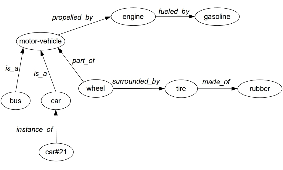
Figure 1: A simple knowledge graph

According to [22], in the following “we use the term semantic relatedness in a general sense, i.e. how much connection humans perceive between two concepts”. Hence, in this paper all kinds of semantic relations have been addressed, without making any assumption about the causes of a given perception.

4 Resource Description Framework (RDF) and DBpedia

The Resource Description Framework (RDF) is a family of specifications designed as a standard model for data interchange on the Web. In particular, RDF is used for the conceptual description or modeling of information of Web resources, each identified by a Uniform Resource Identifier (URI). RDF is based upon the idea of making statements about resources by means of expressions in the form of triples following a subject$-$predicate$-$object pattern. The subject denotes the resource that is being described, and the predicate expresses a relation between the subject and the object, which can be a resource or a literal (e.g., a string, a number).

Let $R=\{r_{1},r_{2},...,r_{n}\}$ be a finite set of URIs each representing a resource, and $L=\{l_{1},l_{2},...,l_{m}\}$ a finite set of literals, an RDF triple (or statement) has the form:

$\langle s,p,o\rangle$,

where s $\in R$ is the subject, p $\in R$ is the predicate, and o $\in R\cup L$ is the object.

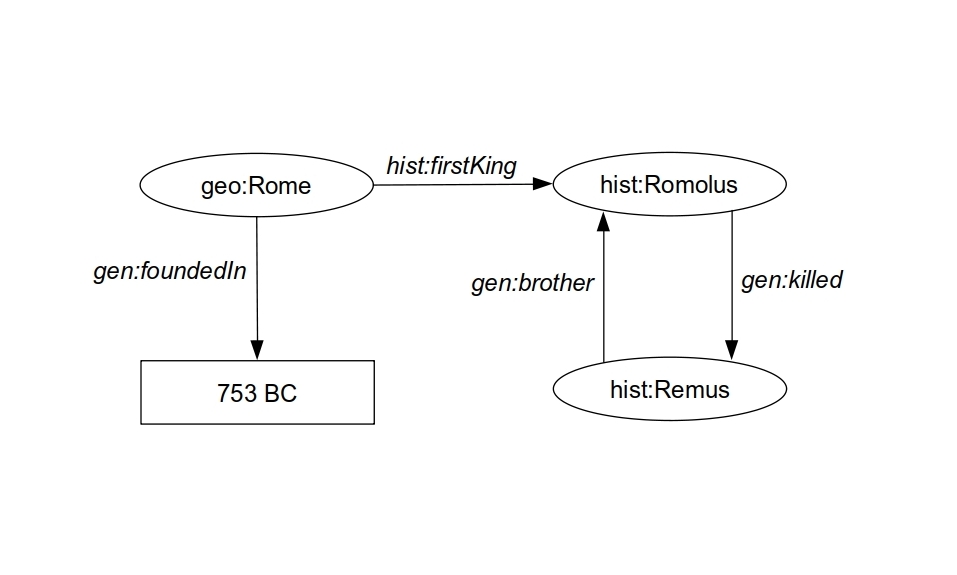
Figure 2: An example of RDF graph

An RDF graph $\mathcal{G}$ is a set of RDF triples, where subjects and objects are nodes, and predicates are directed arcs (also called links, edges or arrows). For instance, in Figure 2 an RDF graph is shown. The triples $\langle\textit{geo:Rome},\textit{hist:firstKing},$ $\textit{hist:Romolus}\rangle$, and $\langle\textit{geo:Rome},\textit{gen:foundedIn},\textit{753 BC}\rangle$ express that the first king of Rome was Romolus, and the city of Rome was founded in 753 before Christ, respectively. In the proposed examples, geo:, hist:, and gen: are prefixes for namespaces that are assumed to contain geographical, historical and generic terms, respectively.

In the following, a triple t $=$ $\langle s,p,o\rangle$ represents a directed link, labelled as p, from the resource s to the resource o. The predicate p is said to be outgoing from s and incoming to o.

Given two resources $r_{a}$ and $r_{b}$, a directed path $P$ of length n from $r_{a}$ to $r_{b}$ is a list of $n$ triples [$t_{1}$, $t_{2}$, … $t_{n}$] where $r_{a}$ coincides with $s_{1}$, the subject of the triple $t_{1}$, $r_{b}$ coincides with $o_{n}$, the object of the triple $t_{n}$, and $o_{i}$, the object of the triple $t_{i}$, coincides with $s_{i+1}$, the subject of the triple $t_{i+1}$, for $1\leq i\leq n-1$. For instance, the sequence of triples [$\langle$geo:Rome, hist:firstKing, hist:Romulus$\rangle$, $\langle$hist:Romulus, gen:killed, hist:Remus$\rangle$] represents a directed path of length $2$, from the resource geo:Rome to the resource hist:Remus.

An undirected path connecting two resources is a path in which the predicates can be traversed in both directions, i.e., they represent undirected links. For instance, the list of triples: [$\langle$geo:Rome, hist:firstKing, hist:Romulus$\rangle$, $\langle$hist:Remus, gen:brother, hist:Romulus$\rangle$] represents an undirected path connecting the resources geo:Rome and hist:Remus, where the predicate gen:brother is traversed from the object hist:Romulus to the subject hist:Remus.

Note that, although an RDF graph can be cyclic, we consider only acyclic paths, i.e., paths where there are no repetitions of nodes, therefore walks [59] are not allowed.

RDF identifies a vocabulary for making assertions on resources. For instance, the predicate rdf:type is used to state that a resource is an instance of another resource. Furthermore, RDF is used for defining further vocabularies. For instance, the RDF Schema (RDFS), and the Web Ontology Language (OWL) are two RDF vocabularies. The former introduces, among the others, the resource rdfs:Class and the predicate rdfs:subClassOf, which can be used for defining taxonomies, whereas the latter, which is built on top of RDFS, defines more sophisticated constructs for representing computational ontologies. Finally, SPARQL, which is a recursive acronym for SPARQL Protocol and RDF Query Language, is an RDF query language based on a SELECT-FROM-WHERE syntax, where variables begin with a question mark (?). For instance, in SPARQL, $\langle r,?x,?y\rangle$ represents any triple having the resource $r$ as subject.

DBpedia is a very huge RDF knowledge graph, and is the result of an ongoing process aimed at semi-automatically extracting information from Wikipedia, in order to represent it in RDF. Therefore, for each Wikipedia article a corresponding RDF resource exists. Note that, a significant part of DBpedia comes from the information in the infoboxes of the Wikipedia articles. The infobox contains data represented as property-value pairs provided by articles’ editors that are, in general, an excerpt of the relevant information of a DBpedia resource.

5 Methods for Computing Semantic Relatedness

In this section, we recall 10 methods for computing semantic relatedness in RDF graphs that have been selected from the literature. These methods have been chosen on the basis of the following criteria:

• They are pure knowledge-based approaches. For this reason, we did not consider any corpus-based and hybrid method and, in general, any method addressing the use of natural language processing techniques.

• They can be applied to any RDF graph, without making any assumption about the types of nodes and predicates. Therefore, we did not take into consideration the methods defined for specific knowledge graphs, as for instance WordNet.

Furthermore, these methods have been identified by:

• Searching on Google Scholar, in September 2021, by using the following keywords: [“semantic relatedness” “rdf”], and by considering only the articles published since 2015.

• Analyzing the first 40 pages of results (400 in total), and by selecting the articles about semantic relatedness methods, according to the above criteria. This search allowed us to identify 4 methods, namely, Linked Data Semantic Distance with Global Normalization (here referred to as LDSDGN) [44], Propagated Linked Data Semantic Distance (PLDSD) [4], Exclusivity-based measure (here referred to as ExclM) [27], and ASRMP_m [13].

• Selecting 6 further methods on the basis of the bibliographic references of the papers about the 4 methods above. These methods are: Wikipedia Link-based Measure (WLM) [63], Linked Open Data Description Overlap (LODDO) [66], Linked Data Semantic Distance (LDSD) [43], IC-based measure (here referred to as ICM) [53], REWOrD [46], and Proximity-based Method (here referred to as ProxM) [32].

In this paper the selected methods have been classified according to the following three groups:

1. Methods based on adjacent resources.

2. Methods based on triple patterns.

3. Methods based on triple weights.

Some of these methods have been originally conceived for computing a distance. Hence, in these cases we adopted the corresponding relatedness formulation, based on the assumption that the shorter the distance the greater the relatedness. In the Appendix the 10 methods are formally recalled and, in order to achieve a more effective comparison among them, a running example is used, based on the graph $\mathcal{G}$ shown in Figure 3. Such a graph contains 13 nodes (resources), linked with directed edges labeled with 4 possible predicates, namely, $p_{1}$, $p_{2}$, $p_{3}$, and rdf:type. Among the 13 resources, $r_{a}$ and $r_{b}$ are the ones whose relatedness will be addressed when describing each method.

Below the 10 methods are informally summarized, and their main characteristics are recalled, but readers interested in the formal aspects can refer to the Appendix.

Figure 3: The running example graph $\mathcal{G}$

5.1 Methods based on adjacent resources

In this subsection the methods belonging to the first group are described, that are based on resources’ adjacent nodes, i.e., nodes that are linked to the compared resources via paths of length 1 in the knowledge graph. They are Wikipedia Link-based Measure (WLM), and Linked Open Data Description Overlap (LODDO).

Wikipedia Link-based Measure (WLM). In [63], the Wikipedia Link-based Measure (WLM) is presented. This measure, which originally exploits the hyperlinks within Wikipedia articles, derives from the well-known Normalized Google Distance ($NGD$) [9], which is based on the assumption that, given two terms, the more pages contain them the more related they are. In this paper, the WLM approach is recalled by applying it to an RDF graph. In particular, rather than considering the Wikipedia articles or Google pages containing a given term, the set of RDF triples of the graph whose objects correspond to such a term are addressed. Then, the set of the resources that are the subjects of such triples are considered.

For instance consider the graph of Figure 3 and the resources $r_{a}$ and $r_{b}$. In order to evaluate their relatedness, two sets of RDF triples have to be addressed, one for each of the compared resources. For example in the case of $r_{a}$, this set is given by the triples of the graph whose objects correspond to such a resource, i.e., {$\langle r_{4},p_{2},r_{a}\rangle$, $\langle r_{9},p_{3},r_{a}\rangle$, $\langle r_{9},p_{1},r_{a}\rangle$, $\langle r_{11},p_{2},r_{a}\rangle$, $\langle r_{b},p_{3},r_{a}\rangle$}. Therefore, regarding $r_{a}$, the set of resources {$r_{4}$, $r_{9}$, $r_{11}$, $r_{b}$} will be considered, i.e., all the resources with incoming predicates to $r_{a}$.

Linked Open Data Description Overlap (LODDO). The Linked Open Data Description Overlap (LODDO) method [66] is based on the notion of description of a resource, which is the set of the resources linked to it, either via an incoming, or an outgoing predicate, excluding rdf:type, and including the resource itself. In other words, a resource r_i, different from $r$, belongs to the description of r if it participates in a triple with r, either as subject or object. For instance, in the graph of Figure 3, the description of $r_{a}$, say $D(r_{a})$, is given by the following set {$r_{a}$, $r_{b}$, $r_{3}$, $r_{4}$, $r_{9}$, $r_{10}$, $r_{11}$}. The approach proposes two strategies, namely LODOverlap and LODJaccard, sharing the rationale that the more the descriptions of two resources have in common, the greater their relatedness. According to [66], the LODOverlap strategy performs better than the LODJaccard one, and this is the strategy that has been considered in our experimentation.

5.2 Methods based on triple patterns

These methods are based on the identification of path patterns in the knowledge graph, i.e., paths satisfying specific conditions with respect to the compared resources. Note that these methods represent distances and, as mentioned above, the shorter the distance the greater the relatedness. They are Linked Data Semantic Distance (LDSD), LDSD with Global Normalization (LDSDGN), and Propagated Linked Data Semantic Distance (PLDSD).

Linked Data Semantic Distance (LDSD). In [43], Passant proposes a theoretical definition of Linked Data and shows how relatedness between resources can be evaluated by using the semantic distance measure introduced by Rada [48]. With respect to the traditional approach of Rada which focuses on hierarchical relations, the proposed distance takes into account any kind of links. In particular, a family of measures for semantic distance has been defined, named Linked Data Semantic Distance (LDSD). In the Appendix, the three measures belonging to this family are recalled. The first one focuses on direct links ($LDSD_{dw}$), the second one on indirect links ($LDSD_{iw}$), and the third one on a combination of both direct and indirect links between the compared resources ($LDSD_{cw}$). As mentioned by the author in [43], among these three measures, the best one is $LDSD_{cw}$, which has been considered in our experiment. In essence, it addresses direct paths, and indirect paths adhering to a specific pattern, that is, two links labeled with the same predicate both outgoing from (incoming to) a third resource and incoming to (outgoing from) the compared resources.

For instance, consider the graph in Figure 3, in comparing the resources $r_{a}$ and $r_{b}$, besides the direct paths, which are [$\langle r_{a},p_{2},r_{b}\rangle$] and [$\langle r_{b},p_{3},r_{a}\rangle$], the following indirect paths contribute: (i) [$\langle r_{4},p_{2},r_{a}\rangle$, $\langle r_{4},p_{2},r_{b}\rangle$], whose links are labeled with $p_{2}$ and are outgoing from the third resource $r_{4}$, (ii) [$\langle r_{11},p_{2},r_{a}\rangle$, $\langle r_{11},p_{2},r_{b}\rangle$], where links are labeled with $p_{2}$ and are outgoing from the third resource $r_{11}$, and (iii) [$\langle r_{a},p_{1},r_{3}\rangle$, $\langle r_{b},p_{1},r_{3}\rangle$], whose links are labeled with $p_{1}$ and are incoming to the third resource $r_{3}$. Note that, as clarified by the formalization of the measures provided in the Appendix, both the $LDSD_{iw}$ and $LDSD_{cw}$ are not symmetric, i.e., they are independent of the order of the compared resources.

LDSD with Global Normalization (LDSDGN). The measures presented in [44], in this paper referred to as LDSD with Global Normalization (LDSDGN), represent an evolution of the approach proposed by Passant [43]. In [44] the authors present three strategies, namely $LDSD_{\alpha}$, $LDSD_{\beta}$, and $LDSD_{\gamma}$. In the first case, they assume that resources are more related if there is a great number of them linked to the compared resources via a given predicate. In the second strategy further assumptions are considered in order to achieve symmetry. In the third case, the contribution of the indirect paths is normalized with respect to the global number of occurrences of the corresponding patterns in the whole graph. According to the authors, $LDSD_{\gamma}$ is the best strategy, and it has been selected for the experiment of this paper.

In the case of the graph of Figure 3, on the basis of the third strategy, the contribution of the path [$\langle r_{a},p_{1},r_{3}\rangle$, $\langle r_{b},p_{1},r_{3}\rangle$], linking $r_{a}$ and $r_{b}$ by means of the predicate $p_{1}$, is normalized by taking into account the cardinality of the set of paths having a similar pattern. In this case, they are two links labeled with $p_{1}$ that are incoming to the same resource, which by chance is always $r_{3}$. In particular, this set is the following:

{[$\langle r_{a},p_{1},r_{3}\rangle$, $\langle r_{5},p_{1},r_{3}\rangle$], [$\langle r_{a},p_{1},r_{3}\rangle$, $\langle r_{6},p_{1},r_{3}\rangle$], [$\langle r_{a},p_{1},r_{3}\rangle$, $\langle r_{b},p_{1},r_{3}\rangle$],

[$\langle r_{b},p_{1},r_{3}\rangle$, $\langle r_{5},p_{1},r_{3}\rangle$], [$\langle r_{b},p_{1},r_{3}\rangle$, $\langle r_{6},p_{1},r_{3}\rangle$], [$\langle r_{5},p_{1},r_{3}\rangle$, $\langle r_{6},p_{1},r_{3}\rangle$]}.

Propagated Linked Data Semantic Distance (PLDSD). The measure proposed in [4] originates from the need to overcome some drawbacks of the families of methods illustrated above. Indeed, according to them, semantic distance is evaluated by focusing on the resources that are either directly or indirectly linked by means of a single intermediate resource. Therefore, all the resources belonging to longer paths are not involved in the relatedness evaluation. For this reason, in the aforementioned paper Alfarhood et al. present a measure, named Propagated Linked Data Semantic Distance (PLDSD), that extends the previous approaches in this direction. In particular, in the proposed method, all the paths between the compared resources, up to a given length $h$, are taken into account, and for each pair of adjacent resources in these paths the original measure of Passant is computed. Therefore, for each triple of a path, the $PLDSD$ method applies the $LDSD_{cw}$ to the pair of resources formed by the subject and the object of the triple. For instance, consider $r_{a}$ and $r_{b}$ in the graph of Figure 3, if we assume $h$ equal to $2$, all the paths linking $r_{a}$ and $r_{b}$ with length not greater than $2$ have to be taken into account. For example, if we focus on the path [$\langle r_{b},p_{3},r_{4}\rangle$, $\langle r_{4},p_{2},r_{a}\rangle$], $LDSD_{cw}$ is applied to the pairs of resources ($r_{b}$, $r_{4}$) and ($r_{4}$, $r_{a}$).

5.3 Methods based on triple weights

In this subsection the third group of methods is described. It concerns five different approaches that, in order to compute semantic relatedness between resources, require the association of weights with triples that allow to evaluate the overall paths. They are Information Content-based Measure (ICM), REWOrD, Exclusivity-based Measure (ExclM), ASRMP_m, and Proximity-based Method (ProxM).

Information Content-based Measure (ICM). The method presented in [53], here referred to as Information Content-based Measure (ICM), relies on the computation of the weights of the triples occurring in the undirected paths connecting the compared resources, up to a given length. The weight is evaluated on the basis of the information content (IC) notion, which needs a probability distribution $P(X)$ over a random variable $X$ to be given, and is defined as $IC(X)$ = $-logP(X)$. The method proposes three strategies, that differ for the adopted probability distribution. The Joint Information Content (jointIC) strategy considers the joint probability of the predicate and the object of a triple by assuming they are not independent, the Combined Information Content (combIC) addresses again the joint probability but the predicates and the objects are supposed to be mutually independent, and the Information Content and Pointwise Mutual Information (IC+PMI) considers the deviation from independence between the predicate and the object. According to the evaluation presented in [53], combIC outperforms the others and, for this reason, it has been considered in the experimentation of the present work.

As an example, in order to weigh the triple $\langle r_{a},p_{2},r_{b}\rangle$ in the graph of Figure 3 by using the combIC strategy, the joint probability of $p_{2}$ and $r_{b}$ needs to be computed. Then, since the strategy assumes that predicates and objects are independent, the required probability is given by the sum of the probabilities of $p_{2}$ and $r_{b}$. In particular, these two probabilities are equal to $\frac{9}{22}$ and $\frac{5}{22}$, where $9$ and $5$ are the numbers of occurrences of the triples with predicate $p_{2}$ and object $r_{b}$, respectively, and $22$ is the total number triples in the graph.

REWOrD. The REWOrD method [46] is based on the notion of informativeness of predicates, which is inspired by the Term Frequency-Inverse Document Frequency (TF-IDF). TF-IDF is commonly used in information retrieval to estimate how important a term w is in a document d belonging to a collection D of documents. When applied to an RDF graph, TF-IDF deals with predicates instead of terms, and resources and triples instead of documents, therefore becomes Predicate Frequency-Inverse Triple Frequency (PF-ITF).

According to this approach, we need to distinguish between outgoing and incoming Predicate Frequency (PF). In particular, the outgoing PF of a predicate $p$ with respect to the resource $r$, say $PF_{o}^{r}(p)$, is the ratio between the number of triples with subject $r$ and predicate $p$, and the number of triples in which $r$ appears either as subject or object. Furthermore, the Inverse Triple Frequency of the predicate $p$, say $ITF(p)$, is equal to the logarithm of the ratio between the total number of triples in the graph and the number of triples with predicate $p$. Then $\textit{PF-}ITF_{o}^{r}(p)$ is defined as the product of $PF_{o}^{r}(p)$ and $ITF(p)$. Analogously, the incoming $\textit{PF-}ITF_{i}^{r}(p)$ of the predicate $p$ with respect to the resource $r$ can be defined.

As a result, the weight of a triple $t=\langle r_{k},p,r_{j}\rangle$, also referred to as the informativeness of $t$, takes into account both the $\textit{PF-}ITF_{o}^{r_{k}}(p)$ and the $\textit{PF-}ITF_{i}^{r_{j}}(p)$.

For instance, consider the triple $\langle r_{a},p_{2},r_{b}\rangle$ of the graph in Figure 3. In order to compute $ITF(p_{2})$, we need: (i) the total number of triples in the graph, that is $22$, and (ii) the number of triples with predicate $p_{2}$, that is $9$. In addition, in order to compute PF${}_{o}^{r_{a}}(p_{2})$, we have to consider: (i) the number of outgoing links from $r_{a}$ with predicate $p_{2}$, that is $2$, and (ii) the number of triples with $r_{a}$ either as subject or object, that is 9. Analogously, in order to compute PF${}_{i}^{r_{b}}(p_{2})$ we have to address: (i) the number of incoming links to $r_{b}$ with predicate $p_{2}$, that is $4$, and (ii) the number of triples with $r_{b}$ either as subject or object, that is $9$.

According to this method, given an undirected path, its informativeness is the sum of the informativeness of the triples of the path divided by the length of the path. In particular, the most informative path (mip) is the path with the greatest informativeness among those connecting the resources, up to a given length.
In order to evaluate the overall relatedness between resources, we need to build their relatedness spaces, i.e., vectors of weighted predicates computed according to five alternative strategies. The first strategy focuses on the incoming predicates, the second one on the outgoing predicates, the third one on both the incoming and the outgoing predicates, the fourth one on the mip, and the fifth one, which has been addressed in the experimentation of this paper (and here referred to as reword), on both the incoming predicates and the mip.

Exclusivity-based Measure (ExclM). The approach proposed in [27], here referred to as Exclusivity-based Measure (ExclM), relies on the notion of exclusivity of triples. The assumption is that, given two resources connected through a predicate, the less the number of resources linked to them through that predicate, the stronger the relation between them. In particular, given a triple $t=\langle r_{i},p,r_{j}\rangle$ in an RDF graph, the exclusivity of $t$, which represents the weight of the triple $t$, is defined as the probability to randomly select the triple $t$ out of the set of all the triples with predicate $p$ and subject $r_{i}$, and all the triples with predicate $p$ and object $r_{j}$.

As an example, in order to associate a weight with the triple $\langle r_{a},p_{2},r_{b}\rangle$ in the graph of Figure 3, two sets of triples have to be considered. In particular, according to the SPARQL notation introduced in Section 4, they are the set of triples of the form $\langle r_{a},p_{2},?x\rangle$, i.e., the ones with the outgoing predicates $p_{2}$ from $r_{a}$, and the set of triples of the form $\langle?x,p_{2},r_{b}\rangle$, i.e., those with the incoming predicate $p_{2}$ to $r_{b}$. Then, on the basis of the triple weights, the set of $k$ undirected paths with the greatest weights between the compared resources are considered. Furthermore, as experimented in the mentioned paper, longer paths contribute less to the relatedness of the compared resources according to a given parameter $\alpha$. In our experiment, $k$ and $\alpha$ are set to $5$ and $0.25$, respectively, since these are the values suggested by the authors.

ASRMP_m. In [13], El Vaigh et al. propose the $ASRMP_{m}$ family of relatedness measures, originating from a previous proposal of the authors, referred to as Weighted Semantic Relatedness Measure ($WSRM$) [12]. They state that a well-founded relatedness measure should meet the following three requirements: (i) to have a formal semantics in order to be defined on a knowledge graph such as RDF or OWL (as opposed to Wikipedia), (ii) to have a reasonable computational cost, (iii) to be transitive, in order to capture directly or indirectly related resources, and symmetric. This family is based on the assumption that the more predicates between resources, the stronger their relatedness. It relies on the $WSRM$ measure of an ordered pair of resources standing for the subject and the object of a given triple. In particular, such a measure is given by the number of outgoing links from the first resource, i.e., the triple’s subject, to the second resource, i.e., the triple’s object, normalized to the total number of outgoing links from the triple’s subject.

For instance, consider the pair of resources $r_{a}$, $r_{b}$ of Figure 3. Then $WSRM(r_{a},r_{b})$ = $\frac{1}{4}$ because there is one direct link from $r_{a}$ to $r_{b}$, and the total number of outgoing links from $r_{a}$ is 4. This family of measures consists of three strategies, namely ASRMP${}_{m}^{a}$, ASRMP${}_{m}^{b}$, ASRMP${}_{m}^{c}$, that consider all the directed paths between the compared resources, where paths and triples are aggregated by using fuzzy logic operators. In particular, the first strategy addresses paths of a given length, say $m$, the second one of length less than or equal to $m$, and the third one also provides a criterion for which paths are weighted depending on their lengths. Since paths are directed, the relatedness of $r_{a}$ to $r_{b}$ is first evaluated and then, in order to achieve symmetry, also the relatedness of $r_{b}$ to $r_{a}$ is computed and their average is considered. In our experiment the ASRMP${}_{m}^{a}$ strategy, which is the best measure according the authors, has been addressed.

Proximity-based Method (ProxM). The Proximity-based Method (ProxM) [32] focuses on the notion of proximity, which has been conceived in order to measure how related two resources are in terms of number of paths between them, rather than addressing the shortest path (distance) between them. A resource may be at the same distance from other resources but it may have more connections (in this proposal undirected paths are considered) with one of them with respect to the others. Therefore, according to the author, the more paths between resources, the higher their proximity. In order to compute it, in this proposal all the paths connecting the resources, up to a maximum length $h$, are considered. However, in general shorter paths contribute more than longer paths. With regard to triple weights, in the experiment given in [32] they are manually assigned, therefore the method does not provide any built-in function for weighing triples.

In Table 1, for each of the 10 methods addressed in the paper, some key aspects are summarized that are: the main features of the method; the contributing links of the compared resources or the contributing paths between them; the maximum distance (Max dist.) between the compared resources in order to have a non-null semantic relatedness degree; whether the method is symmetric (Symm.), i.e., if the order of the resources impacts on the results. Note that, in the case of WLM, LODDO, LDSD, and LDSDGN, if the length of the shortest path between the resources exceeds $2$ their relatedness degree is null, whereas the remaining proposals do not have any constraints about this. Furthermore, all the methods except for LDSD are symmetric.

Table 1: Semantic relatedness methods used in the experiment

	Method	Main features	Contributing	Max	Symm.
	(strategy)	$t=\langle s,p,o\rangle$ is a triple	- links of the compared resources	dist.
		$w(t)$ is the weight of $t$	- paths b/w the compared resources
Adjacent resources	WLM [63]	Inspired by the Normalized Google Distance measure.	All the incoming links.	2	YES
	LODDOa[66]     (LODOverlap)	Overlapping of resources descriptions.	All the incoming and the outgoing links.	2	YES
Triple patterns	LDSDa[43]     (LDSDcw)	Semantic distance between resources.	All the undirected paths with incoming (outgoing) links labeled with the same predicate.	2	NO
	LDSDGNa[44]     (LDSDγ)	Evolution of LDSD with global normalization.	All the undirected paths as in LDSD and extended to the whole graph.	2	YES
	PLDSD [4]	LDSDcw propagated to paths between the compared resources.	The undirected path leading to the shortest distance.	ANY	YES
Triple weights	ICMa[53]                   (combIC)	Information Contents (IC) of predicates and resources.      The weight $w(t)$ is the sum of $IC(p)$ and $IC(o)$.	The undirected path with the greatest weight.	ANY	YES
	REWOrDa[46]     (reword)	Predicate Frequency and Inverse Triple Frequency (PF-ITF). The weight $w(t)$ is the Informativeness of $p$ based on PF-ITF.	The undirected path with the greatest informativeness (mip).	ANY	YES
	ExclM [27]	Longer paths contribute less to the relatedness. The weight $w(t)$ is the probability of selecting a triple out of all those with predicate $p$ and either subject $s$ or object $o$.	The k undirected paths with the greatest weights.	ANY	YES
	$ASRMP_{m}$a[13]     (ASRMP${}_{m}^{a}$)	The more paths the stronger the relatedness.              Fuzzy Logic operators for triple and path aggregations.	All the directed paths.	ANY	YES
		The weight $w(t)$ is the number of links from $s$ to $o$, normalized to the number of outgoing links from $s$.
	ProxM [32]	The more paths the higher the proximity.	All the undirected paths.	ANY	YES
		No built-in function for weighting a triple.

6 Experimentation and Evaluation

In order to evaluate the 10 methods recalled in the previous section, we performed an experimentation by applying them to 14 benchmark golden datasets, and considering a subgraph of the whole DBpedia knowledge graph, as described below. For each dataset, we compared the semantic relatedness values obtained for each method against the human judgment values provided in the dataset. In the next subsections, the portion of the DBpedia knowledge graph and the selected benchmark datasets are outlined. Furthermore, additional details about the set up of the experiment are given and, finally, the evaluation of the methods is illustrated.

6.1 DBpedia data collections used in the experiment

The knowledge graph addressed in the experimentation is a subgraph of the whole DBpedia obtained by considering a subset of its data collections according to the following critera. Firstly, we referred to the most recent version of the essential DBpedia data focused on English. Secondly, we selected all the data collections containing triples having a resource as object rather than a literal. This choice is in line with the one made by all the methods considered in this paper. In the case of data collections containing triples involving literals as objects, such triples have been removed. Thirdly, we selected the data collections containing the triples representing the hyperlinks that appear in the texts of Wikipedia articles. It is important to note that all these triples have the same predicate name, i.e., dbo:wikiPageWikiLink, and correspond to a very huge number in the DBpedia graph. Such triples, although with the same predicate name, gather a relevant piece of information for each resource. Hence, including them in the knowledge graph means to significantly enrich the information provided by the resources’ infoboxes that, often, contain just a summary of the most representative information of a given resource. For instance, the infobox associated with the resource Michael Jackson contains the information related to the dates of his birth and death, the names of his spouses, children, awards, etc. However, it does not specify anything about, for example, the names of his most popular songs, such as Beat It, Billie Jean, or Thriller that, instead, are described in the corresponding Wikipedia article.

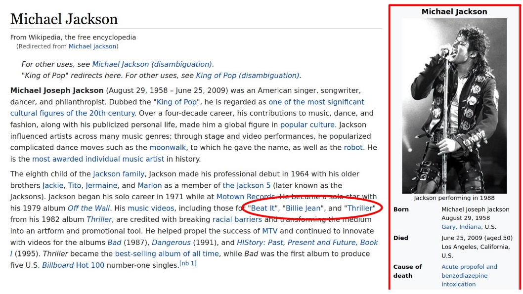
Figure 4: A fragment of the Wikipedia article about Michael Jackson and, on the right side, part of the related infobox

Therefore, excluding the triples with dbo:wikiPageWikiLink as predicate in the experimentation means to have, for each resource, a significantly less number of triples to be evaluated, and hence semantic relatedness is computed by relying on the information provided by the resources’s infoboxes, mainly. For this reason, in order to analyse the relevance of the information contained in the infoboxes in the evaluation of semantic relatedness, we ran two experiments, the first by excluding such triples, and the second by including them. The total dimension of the DBpedia data collections used in the experimentation is around 61 GB, corresponding to 380,891,403 triples. By removing the triples with the dbo:wikiPageWikiLink links, the data decrease to 33 GB, and 207,266,671 triples.

6.2 Benchmark datasets used in the experimentation

Traditionally, computer-aided tasks are evaluated by comparing the behaviour of the computer against the one of human beings. In the case of methods for automatically evaluating semantic relatedness, they are assessed by setting up experiments where people are asked to express numerical values representing how much, according to their opinion, pre-defined pairs of terms are related. These human judgment values are then compared against the automatically computed ones. Such collections of pairs of terms, where each pair is associated with a human judgment value, represent benchmark datasets. In the literature, several benchmark datasets have been defined, often referred to as golden datasets. In this paper, we considered 14 benchmark datasets from the most representative ones presented in [22]. In particular, we selected the datasets in the English language that have been conceived for evaluating semantic relatedness. They are: Atlasify240 (here, Atlasify for short) [24], B₀ (25 pairs) and B₁ (30 pairs) [67], GM30 [21], MTurk287 (here, MTurk for short) [49], Rel122 [55], WRG (252 pairs) [1], and KORE (420 pairs) [25] organized into five datasets, namely, KORE-IT, KORE-HW, KORE-VG, KORE-TV, and KORE-CN. In addition, we included two datasets, namely, RG65 [51] and MC30 [37], which are traditionally considered milestones in order to assess semantic similarity.

It is important to observe that, among the above datasets, all the terms in the KORE collections correspond to DBpedia URIs. All the other datasets contain words that, in some cases, either do not have a straightforward correspondence with a DBpedia resource, or correspond to different DBpedia resources depending on the possible different meanings they have. For this reason, in line with [16], a disambiguation step has been introduced, as described below.

For each word occurrence in a given dataset, the corresponding resource in DBpedia has been manually selected in accordance with the following disambiguation criteria:

• If a word is present in the dataset in a plural form, we transformed it into its singular form.

• If a word in a pair has more than one meaning, and hence can be mapped to more than one DBpedia resource, we selected the resource whose acceptation is more semantically related to the other word of the pair. For instance, the word crain, in the MC30 dataset, leads to two DBpedia resources, namely, http://dbpedia.org/resource/Crane_(bird), and
  http://dbpedia.org/resource/Crane_(machine).
  Hence, in the case of the pair (crain, bird), we selected the first resource, which refers to crane as a bird, whereas in the case of the pair (crain, implementation), we selected the second resource, which refers to crane as a machine [16].

• If a word is a terminological variant, e.g., a synonym, or an acronym, of the name of a given DBpedia resource, for such a word we selected that resource. For instance, in the case of the acronym FBI, we considered the http://dbpedia.org/resource/Federal_Bureau_of_Investigation resource.

According to the above criteria, for each dataset except for the ones in KORE that do not need the disambiguation step, we built another dataset, and in this paper we refer to the former as the original, and to the latter as the disambiguated dataset. Hence, we experimented the methods illustrated in Section 5 on the selected datasets, according to both their original and disambiguated forms.

6.3 Further experimentation details

In the experimentation, for each of the 10 methods we considered the strategy, or variant, that according to the authors provides the best performances. Hence, in the case of LODDO, LDSD, LDSDGN, ICM, REWOrD, ExclM, and $ASRMP_{m}$, we have selected the corresponding variants $LODOverlap$, $LDSD_{cw}$, $LDSD_{\gamma}$, ICM with combIC as weighting function, reword, ExclM with $k=5$ and $\alpha=0.25$, and $ASRMP_{m}^{a}$ with $m=2$. Furthermore, as recalled in Section 5.3 (see also A.3.5), ProxM does not have a built-in function $w(p_{i})$ for weighting a predicate $p_{i}$. In particular, in [32], weights are assigned to predicates by domain experts manually because the graph addressed in the experiment contains a limited number of predicates. However, assigning weights manually is not a scalable approach with respect to the number of predicates in the graph. For this reason, due to the dimension of the DBpedia knowledge graph, in the case of ProxM, in this experiment the weight of a predicate has been defined as its information content, which is a notion that has been attracting a lot of attention in the literature for years [36]. Therefore, we implemented $w(p_{i})=-log(Pr(p_{i}))$, in accordance with the information content definition provided in Eq. 12.

As mentioned, for those methods that natively compute a semantic distance, i.e., WLM, LDSD, LDSDGN, and PLDSD, in the experimentation we consider the corresponding relatedness formulation. In particular, this formulation depends on whether the method returns a value $v$ in the range $[0,\dots,1]$, as for LDSD, LDSDGN, and PLDSD, or in the range $[0,\dots,+\infty)$, as for WLM. In the former case, the corresponding relatedness formulation is defined as $1-v$, whereas in the latter case $\frac{1}{1+v}$.

It is important to recall that, as experimented in [27], in general the longer the paths the weaker the semantic relation, in the sense that the smaller the influence of longer paths, the better the correlation with human judgment. Besides ExclM, this is also the underlying assumption of most of the methods based on triple weights, as for instance ASRMP_m, and it is in line with the implicit assumptions made by WLM and LODDO, which are based on adjacent nodes, and also in line with LDSD and LDSDGN, which rely on patterns represented by paths of length 2. Therefore, in order to compare the 10 methods under the same hypotheses, in our experimentation the length of the contributing paths is not greater than 2.

In the first experiment, the one without the dbo:wikiPageWikiLink links in the knowledge graph, we evaluated the 10 methods also on clean datasets, i.e., the disambiguated datasets where the pairs of terms that are not connected by any path of length less than or equal to 2 have been removed. Whereas, in the experiment including the dbo:wikiPageWikiLink links, clean datasets have not been addressed since there is a limited number of such pairs that can be neglected.

In order to compare the methods against human judgment, we considered both the Spearman’s and Pearson’s correlations. However, for the five KORE datasets we computed only the Spearman’s correlation because for these datasets only pairwise rankings are provided without relatedness values.

In the case of the experiment with the dbo:wikiPageWikiLink links, we also analyzed the performances of the 10 methods when dealing with pairs of disambiguated terms representing common nouns and proper nouns separately. For this purpose, from each dataset we extracted two additional smaller datasets, one containing only pairs of common nouns and the other including only pairs of proper nouns. Then, for each method and each of these additional datasets, we computed the Spearman’s and the Pearson’s correlations against human judgement.

The experimental results are presented and discussed in the next subsection, and all the data are available at [58].

6.4 Evaluation

In this section the results of the two experiments are presented and are shown in Tables 2 and 4, where the Spearman’s and Pearson’s correlations are given, respectively. As mentioned above, the first experiment concerns DBpedia without including the dbo:wikiPageWikiLink links (see columns w/o in the tables, where w/o stands for without dbo:wikiPageWikiLink), whereas in the second experiment these links have been considered (see columns w in the tables, where w stands for with dbo:wikiPageWikiLink). In each table, for each dataset, the results corresponding to the original (o) and disambiguated (d) datasets are shown in the first and the second rows, respectively. In addition, in the first experiment, i.e., the one without dbo:wikiPageWikiLink links, the values obtained by considering the clean datasets (c) are given whereas, as mentioned above, in the second experiment these values have not been considered (see the symbol “$-$” in rows c in the tables). Furthermore, in the tables, the best values are highlighted in bold, and the average correlations (Avg.) for each method are also shown.

Experiment 1: DBpedia without dbo:wikiPageWikiLink links.

In the case the triples with the dbo:wikiPageWikiLink predicate are not considered in the knowledge graph, both the Spearman’s and Pearson’s correlations do not provide satisfactory values (see columns w/o in Tables 2 and 4, respectively). Indeed, for some methods and some datasets, it is not even possible to compute such correlations. For instance, if we consider the $ASRMP_{m}$ method, and the original golden dataset B₀, for any pair of the dataset there are no directed paths of length 2 connecting the related resources, and then the relatedness values returned by the method are null for all the pairs of the dataset (see the symbol “$-$” in the tables). Note that in the case of the Spearman’s correlation (see Table 2), LODDO outperforms the other methods in all the three cases, i.e., with original ($0.34$), disambiguated ($0.49$), and clean datasets ($0.62$). According to Pearson (see Table 4), when the original datasets are considered, LODDO and ExclM provide the highest, although low, results ($0.25$) whereas, in the cases of the disambiguated and clean datasets, LDSD shows the best results by improving its performances from $0.21$ to $0.39$ and $0.50$, respectively.

Overall, the correlation values with human judgment obtained without the dbo: wikiPageWikiLink triples, i.e., by relying mainly on the information of the Wikipedia’s infoboxes, are low. Indeed, the removal of almost half of the triples from the knowledge graph has a great impact on the computation of semantic relatedness because, as shown in the second experiment, although all these triples have the same predicate name, they convey a significant amount of information for each resource that cannot be ignored.

Experiment 2: DBpedia with dbo:wikiPageWikiLink links.

In the presence of the dbo:wikiPageWikiLink predicate, for the majority of the methods both the Spearman’s and Pearson’s correlations significantly increase with respect to the results obtained in the Experiment 1 (see columns w in Tables 2 and 4, respectively). Note that, analogously to the previous experiment, in general the performances of the 10 methods improve by considering the disambiguated datasets. In particular, with regard to the Spearman’s correlation, LODDO outperforms the other methods when the original datasets are addressed ($0.59$) and, overall, the methods based on adjacent resources show good performances. This result is interesting, especially if we consider that the methods based on adjacent resources rely on information that are local to the compared resources, and therefore they require a smaller number of queries and, of course, lower computational complexity costs with respect to the other methods.

It is worth noting that, in the case of the disambiguated datasets, on average, both the methods based on adjacent resources and triples patterns give good results. The role of disambiguation is more evident if we observe the results obtained in Table 2, columns w, for ExclM, with $k=5$ and $\alpha=0.25$, that outperforms the other methods ($0.70$).

In the case of the Pearson’s correlation, for instance, LDSDGN increases of $0.21$, and both WLM and LDSD of $0.18$. Furthermore, it is interesting to observe that ASRMP_m outperforms on average the other methods against both the original ($0.48$) and the disambiguated versions of the datasets ($0.63$). Note that, if we consider the datasets individually, ASRMP_m performs better in half of the cases. More specifically, in the case of the Atlasify, MTurk, and WRG datasets, ASRMP_m provides better results than the other methods, with respect to both the original and the disambiguated versions.

Overall, if compared to the corresponding correlation values obtained without the dbo:wikiPageWikiLink triples, the ASRMP_m method significantly improves its performances. In particular, in the case of disambiguated datasets, it increases on average not only according to Spearman ($0.63$ with respect to $0.21$) but also according to Pearson ($0.63$ with respect to $0.14$). This occurs because this method relies on directed paths, and the absence of such triples implies that several pairs of the compared resources are not connected in the graph, leading therefore to null relatedness degrees. Indeed, ASRMP_m shows the best performance according to the means of the averages of the Spearman’s and Pearson’s correlations with dbo:wikiPageWikiLink triples ($0.63$), as shown in Table 4.

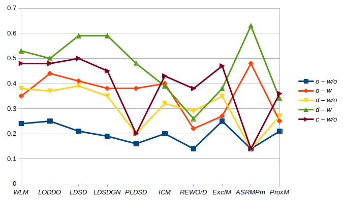
Figure 6: Average Pearson’s correlations line plot

The line plots of the average Spearman’s and Pearson’s correlation values obtained according to the experimental results are shown in Figures 5 and 6, respectively.

As already mentioned, in the case of the Experiment 2, we also studied the correlations of the 10 methods in the presence of disambiguated datasets when only pairs of common nouns or pairs of proper nouns are addressed. Tables 7 and 7 show the experimental results about this further analysis for Spearman and Pearson, respectively. Note that the symbol “$-$” in the tables means that either the corresponding dataset does not contain pairs of a given type (e.g., GM30 does not include any pair of proper nouns) or it is not possible to compute the Spearman’s correlation (as in the case of the KORE datasets for which only pairwise rankings are provided without relatedness values). The experimental results show that, when considering only pairs of common nouns, according to Spearman LODDO outperforms all the other methods ($0.73$), whereas the best Pearson’s correlation is achieved by ASRMP_m ($0.68$). However, if we compute the means of the average Spearman’s and Pearson’s correlations, both ASRMP_m and LODDO show the best performances ($0.65$). In the case of pairs of proper nouns, ExclM provides the best Spearman’s correlation ($0.73$), whereas LDSD shows the best performance according to Pearson ($0.72$). Furthermore, ExclM outperforms the other methods if we consider the means of the average Spearman’s and Pearson’s correlations ($0.69$).

Table 2: Spearman’s correlation for original (o), disambiguated (d), and clean (c) datasets, and DBpedia without dbo:wikiPageWikiLink links (w/o), and with dbo:wikiPageWikiLink links (w)

Dataset	WLM [63]		LODDO [66]		LDSD [43]		LDSDGN [44]		PLDSD [4]		ICM [53]		REWOrD [46]		ExclM [27]		ASRMPm [13]		ProxM [32]
	w/o	w	w/o	w	w/o	w	w/o	w	w/o	w	w/o	w	w/o	w	w/o	w	w/o	w	w/o	w
o	.43	.67	.46	.69	.26	.62	.24	.61	.23	.37	.39	.69	.47	.33	.39	.72	.12	.64	.38	.66
Atlasify d	.43	.62	.46	.66	.23	.58	.20	.57	.23	.33	.37	.66	.44	.29	.37	.68	.12	.62	.35	.64
[24] c	.62	-	.69	-	.35	-	.23	-	.24	-	.68	-	.55	-	.67	-	.08	-	.61	-
o	.32	.36	.29	.68	.14	.40	.16	.35	-	.46	.16	.63	.18	.30	.15	.60	-	.47	.15	.43
B0 d	.53	.70	.60	.76	.42	.67	.44	.67	.25	.48	.44	.76	.36	.62	.43	.79	.25	.75	.40	.59
[67] c	.77	-	.83	-	.84	-	.87	-	.02	-	.90	-	.75	-	.87	-	.20	-	.68	-
o	.16	.30	.13	.23	.00	.17	.00	.19	.31	.11	.01	.28	.21	-.19	.00	.28	.31	.25	.01	.19
B1 d	.33	.69	.48	.66	.26	.48	.18	.55	.31	.34	.48	.71	.38	.16	.38	.72	.31	.56	.42	.54
[67] c	.54	-	.73	-	.53	-	.29	-	.37	-	.79	-	.50	-	.64	-	.37	-	.67	-
o	.22	.44	.23	.69	.25	.46	.25	.47	-	.27	.20	.67	.15	.40	.21	.63	-	.58	.21	.58
GM30 d	.22	.54	.50	.79	.48	.72	.46	.59	.16	.40	.45	.78	.42	.28	.46	.82	.00	.65	.43	.69
[21] c	.19	-	.65	-	.61	-	.59	-	.07	-	.61	-	.31	-	.65	-	.00	-	.48	-
o	.15	.41	.21	.49	.26	.43	.26	.41	.14	.37	.22	.46	.20	.29	.23	.48	.14	.45	.21	.45
MTurk d	.24	.51	.32	.49	.28	.49	.28	.47	.22	.36	.29	.52	.23	.23	.29	.53	.19	.52	.26	.51
[49] c	.22	-	.37	-	.36	-	.30	-	.26	-	.39	-	.33	-	.37	-	.23	-	.18	-
o	.15	.39	.17	.46	.08	.33	.07	.36	.02	.35	.10	.41	.19	.31	.11	.44	.02	.39	.01	.39
Rel122 d	.25	.66	.36	.65	.17	.58	.15	.57	.09	.48	.26	.61	.12	.30	.27	.66	.09	.58	.25	.57
[55] c	.32	-	.55	-	.20	-	.06	-	.09	-	.41	-	.19	-	.53	-	.09	-	.36	-
o	.25	.33	.26	.46	.14	.33	.14	.37	.18	.42	.24	.46	-.03	.00	.24	.47	.16	.47	.24	.41
WRG d	.32	.51	.33	.58	.18	.44	.19	.49	.20	.39	.29	.55	.14	.09	.29	.57	.15	.54	.29	.56
[1] c	.40	-	.45	-	.18	-	.26	-	.29	-	.50	-	.06	-	.52	-	.20	-	.56	-
o	.19	.36	.23	.68	.18	.40	.18	.35	.32	.46	.21	.63	.21	.30	.20	.60	.20	.50	.21	.54
RG65 d	.55	.70	.62	.76	.54	.67	.55	.67	.24	.48	.58	.76	.52	.62	.58	.79	.00	.75	.58	.75
[51] c	.70	-	.78	-	.66	-	.68	-	.20	-	.77	-	.66	-	.77	-	.00	-	.78	-
o	.08	.16	.01	.54	-.18	.26	-.19	.15	.33	.26	-.09	.45	.09	.23	-.11	.42	.33	.42	-.09	.30
MC30 d	.35	.81	.36	.86	.16	.76	.17	.76	.20	.30	.25	.81	.28	.54	.25	.79	.23	.79	.25	.80
[37] c	.64	-	.75	-	.52	-	.58	-	.00	-	.73	-	.54	-	.76	-	.00	-	.73	-
o	.49	.63	.69	.76	.51	.68	.06	.32	.65	-.01	.64	.62	.40	-.06	.62	.75	.57	.65	.58	.68
KORE-IT d	.49	.63	.69	.76	.51	.68	.06	.32	.65	-.01	.64	.62	.40	-.06	.62	.75	.57	.65	.58	.68
[25] c	.49	-	.69	-	.51	-	.06	-	.65	-	.64	-	.40	-	.62	-	.57	-	.58	-
o	.33	.53	.61	.52	.62	.73	.32	.44	.63	-.08	.62	.66	.46	.37	.59	.71	.31	.54	.62	.72
KORE-HW d	.33	.53	.61	.52	.62	.73	.32	.44	.63	-.08	.62	.66	.46	.37	.59	.71	.31	.54	.62	.72
[25] c	.33	-	.61	-	.62	-	.32	-	.63	-	.62	-	.46	-	.59	-	.31	-	.62	-
o	.42	.70	.51	.60	.19	.48	.35	.51	.33	-.11	.44	.54	.27	.10	.49	.67	.36	.62	.43	.56
KORE-VG d	.42	.70	.51	.60	.19	.48	.35	.51	.33	-.11	.44	.54	.27	.10	.49	.67	.36	.62	.43	.56
[25] c	.42	-	.51	-	.19	-	.35	-	.33	-	.44	-	.27	-	.49	-	.36	-	.43	-
o	.54	.64	.45	.71	.39	.61	-.01	.43	.53	.01	.48	.68	.19	-.41	.46	.62	.18	.59	.46	.70
KORE-TV d	.54	.64	.45	.71	.39	.61	-.01	.43	.53	.01	.48	.68	.19	-.41	.46	.62	.18	.59	.46	.70
[25] c	.54	-	.45	-	.39	-	-.01	-	.53	-	.48	-	.19	-	.46	-	.18	-	.46	-
o	.53	.69	.55	.73	.34	.59	-.13	.38	.43	.37	.42	.49	.13	.09	.47	.74	.13	.66	.28	.65
KORE-CN d	.53	.69	.55	.73	.34	.59	-.13	.38	.43	.37	.42	.49	.13	.09	.47	.74	.13	.66	.28	.65
[25] c	.53	-	.55	-	.34	-	-.13	-	.43	-	.42	-	.13	-	.47	-	.13	-	.28	-
o	.30	.47	.34	.59	.23	.46	.12	.38	.27	.23	.29	.55	.22	.15	.29	.58	.20	.52	.26	.53
Avg. d	.40	.64	.49	.68	.34	.61	.23	.53	.32	.27	.43	.65	.31	.23	.43	.70	.21	.63	.40	.65
c	.48	-	.62	-	.45	-	.32	-	.29	-	.60	-	.38	-	.60	-	.19	-	.53	-

Table 3: Pearson’s correlation for original (o), disambiguated (d), and clean (c) datasets, and DBpedia without dbo:wikiPageWikiLink links (w/o), and with dbo:wikiPageWikiLink links (w)

Dataset	WLM [63]		LODDO [66]		LDSD [43]		LDSDGN [44]		PLDSD [4]		ICM [53]		REWOrD [46]		ExclM [27]		ASRMPm [13]		ProxM [32]
	w/o	w	w/o	w	w/o	w	w/o	w	w/o	w	w/o	w	w/o	w	w/o	w	w/o	w	w/o	w
o	.42	.58	.27	.49	.40	.60	.31	.57	.19	.48	.19	.21	.51	.33	.34	.35	.15	.62	.09	.09
Atlasify d	.42	.51	.27	.49	.40	.58	.29	.53	.19	.41	.19	.19	.48	.28	.34	.35	.15	.61	.09	.09
[24] c	.55	-	.33	-	.50	-	.32	-	.19	-	.20	-	.55	-	.43	-	.15	-	.12	-
o	.35	.55	.31	.47	.36	.51	.36	.52	-	.35	.27	.47	.24	.15	.34	.35	-	.47	.34	.35
B0 d	.55	.63	.57	.62	.57	.66	.61	.69	.26	.45	.53	.59	.33	.11	.51	.51	.26	.62	.46	.52
[67] c	.68	-	.73	-	.75	-	.86	-	.29	-	.84	-	.76	-	.62	-	.29	-	.53	-
o	.22	.33	.33	.46	.30	.33	.20	.28	.30	.23	.23	.35	.14	-.16	.36	.37	.30	.45	.30	.30
B1 d	.41	.57	.42	.49	.41	.57	.22	.54	.30	.33	.31	.31	.32	.16	.40	.44	.30	.74	.27	.27
[67] c	.57	-	.46	-	.57	-	.42	-	.37	-	.25	-	.25	-	.49	-	.32	-	.20	-
o	.29	.46	.28	.45	.34	.50	.34	.51	-	.49	.27	.30	.01	.36	.29	.31	-	.53	.27	.27
GM30 d	.29	.34	.32	.47	.43	.63	.38	.58	.14	.65	.29	.31	.37	.19	.31	.34	.00	.51	.27	.27
[21] c	.32	-	.47	-	.55	-	.44	-	.13	-	.42	-	.34	-	.45	-	.00	-	.41	-
o	.17	.38	.26	.28	.26	.43	.22	.42	.16	.42	.25	.49	.21	.28	.20	.22	.14	.50	.10	.17
MTurk d	.25	.42	.22	.31	.33	.48	.29	.52	.24	.36	.18	.20	.28	.23	.21	.13	.16	.58	.15	.15
[49] c	.19	-	.25	-	.36	-	.28	-	.26	-	.20	-	.33	-	.23	-	.17	-	.18	-
o	.17	.37	.20	.39	.12	.32	.15	.36	.04	.38	.14	.39	.14	.30	.16	.21	.04	.37	.15	.18
Rel122 d	.26	.66	.32	.48	.26	.56	.22	.57	.08	.59	.29	.57	.09	.32	.25	.29	.08	.53	.24	.37
[55] c	.32	-	.47	-	.31	-	.24	-	.10	-	.45	-	.23	-	.35	-	.10	-	.31	-
o	.23	.22	.18	.39	.18	.33	.18	.37	.16	.40	.24	.38	.01	.15	.16	.17	.14	.44	.14	.17
WRG d	.29	.33	.16	.32	.24	.41	.24	.48	.17	.40	.09	.12	.17	.24	.20	.21	.15	.50	.03	.03
[1] c	.41	-	.19	-	.33	-	.31	-	.20	-	.07	-	.16	-	.28	-	.21	-	.02	-
o	.20	.26	.29	.56	.20	.47	.17	.32	.32	.43	.27	.60	.09	.23	.20	.21	.19	.51	.22	.30
RG65 d	.57	.57	.60	.63	.58	.68	.57	.66	.25	.62	.56	.57	.42	.44	.52	.52	.00	.74	.55	.75
[51] c	.70	-	.78	-	.66	-	.68	-	.20	-	.77	-	.66	-	.77	-	.00	-	.78	-
o	.08	.05	.12	.48	-.26	.24	-.19	.10	.26	.26	-.05	.42	-.10	.32	.20	.25	.26	.44	.26	.46
MC30 d	.37	.75	.43	.70	.27	.70	.32	.75	.20	.54	.41	.65	.11	.34	.43	.63	.18	.80	.41	.64
[37] c	.55	-	.68	-	.47	-	.53	-	.08	-	.66	-	.14	-	.64	-	.00	-	.65	-
o	-	-	-	-	-	-	-	-	-	-	-	-	-	-	-	-	-	-	-	-
KORE d	-	-	-	-	-	-	-	-	-	-	-	-	-	-	-	-	-	-	-	-
[25] c	-	-	-	-	-	-	-	-	-	-	-	-	-	-	-	-	-	-	-	-
o	.24	.35	.25	.44	.21	.41	.19	.38	.16	.38	.20	.40	.14	.22	.25	.27	.14	.48	.21	.25
Avg. d	.38	.53	.37	.50	.39	.59	.35	.59	.20	.48	.32	.39	.29	.26	.35	.38	.14	.63	.27	.34
c	.48	-	.48	-	.50	-	.45	-	.20	-	.43	-	.38	-	.47	-	.14	-	.36	-

Table 4: Means of the average Spearman’s and Pearson’s correlations for disambiguated datasets and DBpedia with dbo:wikiPageWikiLinks links

WLM [63]	LODDO [66]	LDSD [43]	LDSDGN [44]	PLDSD [4]	ICM [53]	REWOrD [46]	ExclM [27]	ASRMPm [13]	ProxM [32]
.59	.59	.60	.56	.38	.52	.25	.54	.63	.50

Table 5: Spearman’s correlation for common nouns (c) and proper nouns (p) in disambiguated datasets and DBpedia with dbo:wikiPageWikiLinks links

Dataset	WLM [63]		LODDO [66]		LDSD [43]		LDSDGN [44]		PLDSD [4]		ICM [53]		REWOrD [46]		ExclM [27]		ASRMPm [13]		ProxM [32]
	c	p	c	p	c	p	c	p	c	p	c	p	c	p	c	p	c	p	c	p
Atlasify[24]	.70	.80	.77	.79	.74	.73	.64	.91	.45	.50	.76	.90	.51	.56	.69	.84	.70	.92	.68	.92
B0[67]	.51	.89	.92	.85	.92	.81	.92	.86	.79	.24	.92	.82	.54	.59	.81	.92	.87	.49	.95	.62
B1[67]	.40	.64	.70	.38	.80	.40	.10	.25	.87	-.22	-.21	.59	.30	-.34	.00	.62	.11	.44	.16	.27
GM30[21]	.54	-	.79	-	.72	-	.59	-	.40	-	.78	-	.28	-	.82	-	.65	-	.69	-
MTurk[49]	.47	-.07	.56	-.24	.47	.38	.47	.28	.42	.38	.53	.20	.30	-.32	.54	.25	.50	.25	.53	.32
Rel122[55]	.66	-	.65	-	.58	-	.57	-	.48	-	.61	-	.30	-	.66	-	.58	-	.57	-
WRG[1]	.52	1.0	.57	1.0	.44	1.0	.50	1.0	.40	1.0	.54	1.0	.08	1.0	.56	1.0	.53	1.0	.55	1.0
RG65[51]	.70	-	.76	-	.67	-	.67	-	.48	-	.76	-	.62	-	.79	-	.75	-	.75	-
MC30[37]	.81	-	.86	-	.76	-	.76	-	.30	-	.81	-	.54	-	.79	-	.79	-	.80	-
KORE-IT[25]	-	.63	-	.76	-	.68	-	.32	-	-.01	-	.62	-	-.06	-	.75	-	.65	-	.68
KORE-HW[25]	-	.53	-	.52	-	.73	-	.44	-	-.08	-	.66	-	.37	-	.71	-	.54	-	.72
KORE-VG[25]	-	.70	-	.60	-	.48	-	.51	-	-.11	-	.54	-	.10	-	.67	-	.62	-	.43
KORE-TV[25]	-	.69	-	.73	-	.59	-	.38	-	.37	-	.49	-	.09	-	.74	-	.66	-	.65
KORE-CN[25]	-	.69	-	.73	-	.59	-	.38	-	.37	-	.49	-	.09	-	.74	-	.66	-	.65
Avg.	.59	.65	.73	.56	.68	.66	.58	.66	.51	.38	.61	.70	.39	.30	.63	.73	.61	.62	.63	.62

Table 6: Pearson’s correlation for common nouns (c) and proper nouns (p) in disambiguated datasets and DBpedia with dbo:wikiPageWikiLinks links

Dataset	WLM [63]		LODDO [66]		LDSD [43]		LDSDGN [44]		PLDSD [4]		ICM [53]		REWOrD [46]		ExclM [27]		ASRMPm [13]		ProxM [32]
	c	p	c	p	c	p	c	p	c	p	c	p	c	p	c	p	c	p	c	p
Atlasify[24]	.56	.63	.48	.81	.66	.88	.65	.61	.54	.35	.21	.78	.44	.55	.36	.70	.65	.91	.13	.45
B0[67]	.54	.74	.82	.83	.72	.79	.82	.76	.86	.35	.75	.82	.43	.41	.67	.57	.89	.60	.67	.58
B1[67]	.54	.59	.98	.88	.03	.59	.84	.22	.59	-.01	-.61	.53	.43	-.35	-.51	.67	.97	.69	-.34	.55
GM30[21]	.34	-	.47	-	.63	-	.58	-	.65	-	.31	-	.19	-	.34	-	.51	-	.27	-
MTurk[49]	.40	.29	.32	-.32	.50	.35	.51	-.10	.49	.10	.57	.10	.32	-.16	.19	.37	.55	.22	.42	.37
Rel122[55]	.66	-	.48	-	.56	-	.57	-	.59	-	.57	-	.32	-	.29	-	.53	-	.37	-
WRG[1]	.26	1.0	.31	1.0	.42	1.0	.49	1.0	.39	1.0	.12	1.0	.23	1.0	.20	1.0	.52	1.0	.04	1.0
RG65[51]	.57	-	.63	-	.68	-	.66	-	.62	-	.57	-	.44	-	.52	-	.74	-	.75	-
MC30[37]	.75	-	.70	-	.70	-	.45	-	.54	-	.65	-	.34	-	.63	-	.80	-	.64	-
KORE[25]	-	-	-	-	-	-	-	-	-	-	-	-	-	-	-	-	-	-	-	-
Avg.	.51	.65	.58	.64	.54	.72	.62	.50	.59	.36	.35	.65	.35	.29	.30	.66	.68	.68	.33	.59

Table 7: Means of the average Spearman’s and Pearson’s correlations for common nouns (c) and proper nouns (p) in disambiguated datasets and DBpedia with dbo:wikiPageWikiLinks links

	WLM [63]	LODDO [66]	LDSD [43]	LDSDGN [44]	PLDSD [4]	ICM [53]	REWOrD [46]	ExclM [27]	ASRMPm [13]	ProxM [32]
c	.55	.65	.61	.60	.55	.48	.37	.46	.65	.48
p	.65	.63	.68	.52	.30	.64	.25	.69	.65	.61

Figure 5: Average Spearman’s correlations line plot

6.4.1 Discussion

On the basis of the experimentation of this work, the ASRMP_m method shows the best performance by considering disambiguated datasets and DBpedia with the dbo:wikiPageWikiLink predicate. Indeed, a peculiarity of this method consists in taking into account all the directed paths connecting two resources, rather than selecting one or more of them according to some criteria (see Eq. 26 in the Appendix). In fact, by summarizing, the WLM method, rather than addressing paths, relies on the information gathered by the nodes that are adjacent to the compared resources. The same also holds in the case of LODDO although, according to the assumptions made, it implicitly considers all the paths of maximum length 2, both directed and undirected. With regard to the methods based on triple patterns, namely LDSD, LDSDGN, and PLDSD, they aim at verifying the existence of specific configurations of paths, involving further resources in the graph on the basis of the names of the triples’ predicates. Among these methods, only PLDSD addresses all the paths, directed and undirected, between the compared resources. Finally, among the methods based on triple weights, ICM focuses on the information contents of both the predicates and the objects of the triples and, analogously, ProxM that, according to the assumptions made in order to implement it, relies on the information contents of the triples’ predicates. REWOrD selects the most informative path among the ones connecting the compared resources, whereas ExclM focuses on the top-k undirected paths between the compared resources. Therefore, aggregating all the directed paths between resources is a distinctive feature of ASRMP_m that contributes to make it the best strategy in order to compute semantic relatedness in the presence of datasets containing both common nouns and proper nouns.

In addition, overall ASRMP_m and LODDO show the best performances by considering only pairs of common nouns from disambiguated datasets, whereas ExclM outperforms the other methods when addressing only pairs of proper nouns.

With regard to time complexity, as mentioned, the motivation of this work is a comparison about the correlations of the methods with human judgment by running them all at once against the same datasets, and on the same DBpedia release. For this reason, in this paper, the complexity analysis of the methods has not been given (when present, it can be found in the original papers where the methods have been proposed). About the running times, we ran the experimentation on a machine with 32GB of RAM and the Intel® Core™ i7-8665U CPU @ 1.90GHz $\times$ 8 octa-core processor. In Table 8, for each method, the worst running times needed in order to compute the relatedness of a single pair of resources are shown. In particular, in the table the worst running times for a pair of common nouns and a pair of proper nouns are distinguished. Such times for common nouns are in general significantly less than the ones needed for evaluating the relatedness of proper nouns. In fact, usually, in DBpedia nodes labeled with common nouns are involved in less triples than nodes representing proper nouns.

Table 8: Worst running times (in seconds) for a single pair of common (c) and proper nouns (p)

Method	c	p
WLM [63]	0.6	1.1
LODDO [66]	0.4	0.5
LDSD [43]	11.8	21.0
LDSDGN [44]	5.9	9.0
PLDSD [4]	96.3	840.1
ICM [53]	7.3	8.7
REWOrD [46]	6.3	17.5
ExclM [27]	9.9	78.1
ASRMPm [13]	0.4	1.5
ProxM [32]	9.2	12.6

Table 9: Pros and Cons of the methods where $d$ is the distance between the compared resources

Method	Pros	Cons
WLM	- running time - straightforward	- local - predicates are not addressed - null relatedness values if $d$ $>$ $2$
LODDO	- running time - straightforward - the best overall correlation for common nouns	- local - predicates are not addressed - null relatedness values if $d$ $>$ $2$
LDSD	- straightforward - more selectivity	- null relatedness values if $d$ $>$ $2$
LDSDGN	- global - more selectivity	- non-straightforward - complex formalization - null relatedness values if $d$ $>$ $2$
PLDSD	- non-null relatedness values for any $d$	- running time - less selectivity - the worst overall correlation for proper nouns
ICM	- global - non-null relatedness values for any $d$	- less selectivity
REWOrD	- global - non-null relatedness values for any $d$	- non-straightforward - less selectivity - the worst overall correlation - the worst overall correlation for common nouns
ExclM	- straightforward - non-null relatedness values for any $d$ - the best overall correlation for proper nouns	- tuning parameters - less selectivity
ASRMPm	- running time - more selectivity - non-null relatedness values for any $d$ - the best overall correlation - the best overall correlation for common nouns	- non-intuitive fuzzy logic operators for triple and path aggregations
ProxM	- global - non-null relatedness values for any $d$	- no built-in functions to weigh triples - less selectivity

In Table 9, pros and cons of the 10 methods are shown. In the table, $d$ is the distance between the compared resources, as defined according to the standard notion of shortest-path distance in graph theory. For “straightforward” we mean that the approach is intuitive and easy to implement, whereas “complex formalization” is related to the complexity of the underlying formulas (that are shown in the Appendix). “Local” means that the method focuses on the information provided by the nodes that are adjacent to the compared resources, whereas “global” implies that the information contained in the whole graph is addressed. Furthermore, “more selectivity” stands for methods defining some criteria in order to detect the kinds of paths to be considered (as for instance ASRMP_m, which focuses on directed paths, or LDSD and LDSDGN that leverage specific path configurations), whereas “less selectivity” means that any path is considered a priori. Overall, in the case of ASRMP_m, we observe an imbalance in favor of pros with respect to cons, taking into account in particular the running times, the focus on directed paths that is a proper characteristic of this approach, and the best overall correlations in general, and in the specific case of common nouns from disambiguated datasets.

7 Conclusion

Evaluating semantic relatedness of resources in RDF knowledge graphs is still a challenge. In this paper, 10 methods have been selected and experimented against 14 benchmark golden datasets by using DBpedia as reference RDF knowledge graph. The 10 approaches have been organized according to three representative groups, namely, the methods based on adjacent resources, triple patters, and triple weights, and their differences and commonalities have been highlighted.

The experimental results show that, first of all, the disambiguation of the dataset plays a fundamental role in evaluating semantic relatedness. Furthermore, the triples with the dbo:wikiPageWikiLink predicate represent a significant integration to the information provided by the resources’ infoboxes, that contain partial summaries of the most important data associated with the resources. Finally, with regard to the methods, according to the experimental results, overall the strategy relying on triple weights, when combined with the evaluation of all the directed paths connecting the compared resources, shows the best performances.

It is important to recall that in this experiment, when for a given method more than one strategy, or variant, is present, we have considered the one that the authors identify as the best strategy in order to evaluate semantic relatedness. However, in some cases we realized that in our experiment the best variant for the authors does not correspond to the one associated with the best correlation values. For this reason, as a future work, we are planning to run a wider experimentation where all the strategies of the methods are addressed (approximately 30 in total) and compared.

8 Funding

This research did not receive any specific grant from funding agencies in the public, commercial, or not-for-profit sectors.

Appendix

Appendix A The 10 selected methods

In this Appendix, the 10 selected methods are described in details, and are compared by using a running example based on the graph $\mathcal{G}$ shown in Figure 3. As mentioned above, it contains 13 nodes (resources), linked with directed edges labeled with the predicates $p_{1}$, $p_{2}$, $p_{3}$, and rdf:type. For each method, $r_{a}$ and $r_{b}$ are the resources whose relatedness will be addressed in order to highlight the specific characteristics of the different approaches.

A.1 Methods based on adjacent resources

In the following the methods based on adjacent resources are described.

A.1.1 Wikipedia Link-based Measure (WLM)

According to [63], consider an RDF graph $\mathcal{G}$, and the set $R$ of all the resources as defined according to the notation recalled in Section 4. Assume $r_{a}$, $r_{b}$ $\in$ $R$, and let $A$, $B$ be the sets of the resources that are subjects of the triples with $r_{a}$ and $r_{b}$ as objects, respectively, i.e.:

$A=\{r_{j}\in R|\exists p_{i}:\langle r_{j},p_{i},r_{a}\rangle\in\mathcal{G}\}$, $B=\{r_{j}\in R|\exists p_{i}:\langle r_{j},p_{i},r_{b}\rangle\in\mathcal{G}\}$

According to the SPARQL notation introduced above, the sets $A$, and $B$ can also be rewritten as follows:

$A=\{?x|\langle?x,?y,r_{a}\rangle\in\mathcal{G}\}$, $B=\{?x|\langle?x,?y,r_{b}\rangle\in\mathcal{G}\}$

The WLM measure between the resources $r_{a}$ and $r_{b}$, $WLM(r_{a},r_{b})$, is a distance rather than a relatedness measure since it originates from the Normalized Google Distance, and is defined according to Eq. 1:

$$WLM(r_{a},r_{b})=\frac{log(max(|A|,|B|))-log(|A\cap B|)}{log(|R|)-log(min(|A|,|B|))}$$ (1)

where, for any set $S$, $|S|$ is the cardinality of $S$. Note that, in the case both $r_{a}$ and $r_{b}$ never occur as object in any triple, $WLM(r_{a},r_{b})=\frac{\infty}{\infty}$ = 1 is assumed. Furthermore, if $r_{a}$ and $r_{b}$ are linked to the same resources or $r_{a}$ $\equiv$ $r_{b}$, then $A\equiv B$, therefore their distance is null ($WLM(r_{a},r_{b})$ = 0). In the case $WLM$ $\geq$ 1, $r_{a}$ and $r_{b}$ are very unrelated and, in particular, if there are no resources linked to both $r_{a}$ and $r_{b}$, their distance is infinite ($WLM(r_{a},r_{b})$ = $\infty$), and they provide the minimum relatedness degree. Since $WLM$ ranges in the interval $[0,\dots,+\infty)$, in this paper in order to experiment and compare it against the other methods, the relatedness formulation $\frac{1}{1+WLM}$ has been used.

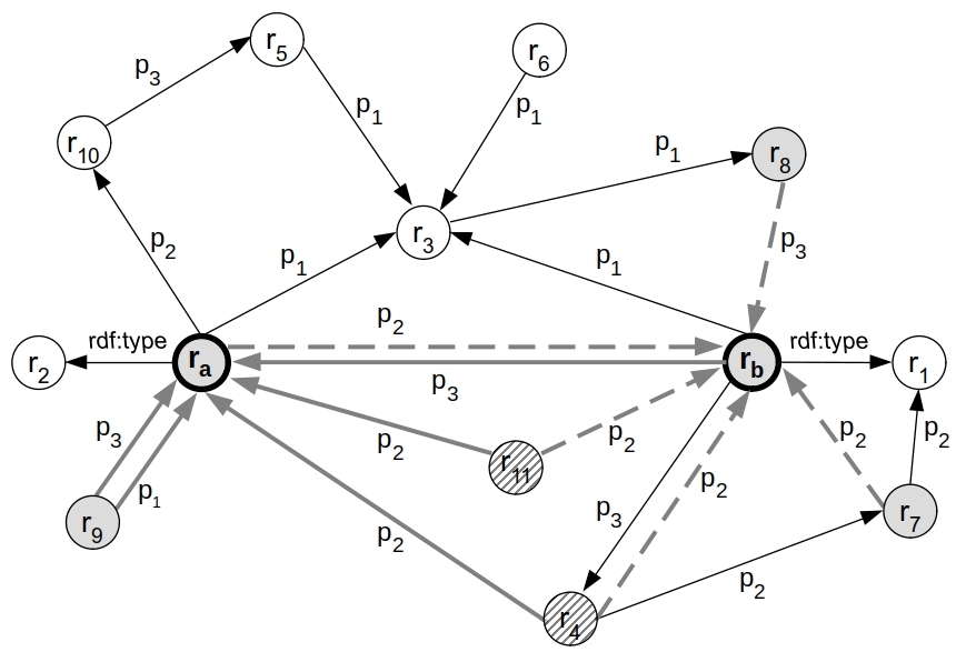
Figure 7: WLM applied to the running example graph

For instance, consider the nodes labeled with the resources $r_{a}$ and $r_{b}$ of the graph shown in Figure 3. In order to evaluate the relatedness of $r_{a}$ and $r_{b}$ according to WLM, only the nodes (resources) with outgoing predicates towards $r_{a}$ and $r_{b}$ are considered, that are represented by the sets A = {$r_{4}$, $r_{9}$, $r_{11}$, $r_{b}$}, and B = {$r_{4}$, $r_{7}$, $r_{8}$, $r_{11}$, $r_{a}$}, respectively. In Figure 7, the related links are highlighted with bold grey arrows, and long dashed grey arrows, respectively. In particular, the nodes $r_{4}$ and $r_{11}$, having outgoing predicates towards both $r_{a}$ and $r_{b}$ (the intersection of A and B) are filled with upward diagonals, whereas the nodes of all the other involved resources are in grey. Note that the resource $r_{9}$, although having two outgoing predicates towards $r_{a}$, appears only once because A is a set.

A.1.2 Linked Open Data Description Overlap (LODDO)

As mentioned in Section 5.1, the Linked Open Data Description Overlap (LODDO) method is based on the notion of resource’s description [66]. Given a resource r, the description $D$ of r, $D(r)$, is the set of the resources r_i that are directly linked to r, either via an incoming, or an outgoing predicate, plus the resource r itself. Furthermore, the method does not include in $D(r)$ all the resources that are linked to $r$ via the predicate rdf:type, exclusively. This is because, according to the authors of the method, given an RDF knowledge graph, almost every resource has owl:Thing as type, and therefore the type assertions are considered “noisy links” that have to be ignored. The description $D$ of the resource $r$, $D(r)$, can be formally defined according to the SPARQL notation as follows:

$$D(r)= \{?r_{i}|\langle r,?p_{j},?r_{i}\rangle\text{ $\in$ }\mathcal{G},?p_{j}\neq\textit{rdf:type}\}\cup$$ (2)

$$\{?r_{i}|\langle?r_{i},?p_{j},r\rangle\text{ $\in$ }\mathcal{G},?p_{j}\neq\textit{rdf:type}\}$$

For instance, if we consider the resources $r_{a}$ and $r_{b}$ of our running example, $D(r_{a})=\{r_{a},r_{b},r_{3},r_{4},r_{9},r_{10},r_{11}\}$, and $D(r_{b})=\{r_{b},r_{a},r_{3},r_{4},r_{7},r_{8},r_{11}\}$. In Figure 8, the links that contribute to the descriptions of $r_{a}$ and $r_{b}$ are depicted as long dashed grey arrows and dashed grey arrows, respectively, whereas the links that contribute to the description of both the resources are in bold grey. Furthermore, the nodes in $D(r_{a})$ and $D(r_{b})$ have been highlighted. It is worth noting that the resources $r_{2}$ and $r_{1}$ are not included in the above descriptions, since they are linked to $r_{a}$ and $r_{b}$ via the rdf:type predicate only, respectively.

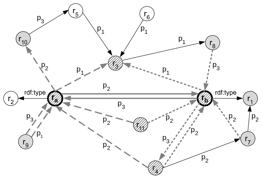
Figure 8: LODDO applied to the running example graph

Given two resources, say $r_{a}$ and $r_{b}$, the following two strategies for computing the semantic relatedness between them are proposed, namely, LODJaccard and LODOverlap:

LODOverlap. The LODOverlap has a bias towards the resource, between the two, with a less rich description (Eq. 3), where $min$ stands for the minimum cardinality between the descriptions of $r_{a}$ and $r_{b}$.

$$LODOverlap(r_{a},r_{b})=\frac{|D(r_{a})\cap D(r_{b})|}{min\{|D(r_{a})|,|D(r_{b})|\}}$$ (3)

LODJaccard. $LODJaccard$ resembles the $Jaccard$ similarity coefficient [29], making no distinction between the two resources (Eq. 4). In fact, in place of the minimum, both the cardinalities of the descriptions are addressed.

$$LODJaccard(r_{a},r_{b})=\frac{|D(r_{a})\cap D(r_{b})|}{|D(r_{a})|+|D(r_{b})|-|D(r_{a})\cap D(r_{b})|}$$ (4)

For both the strategies, the bigger the intersection between the descriptions of the compared resources the higher their semantic relatedness degree.

The method does not explicitly search for paths linking $r_{a}$ and $r_{b}$. However, the semantic relatedness between $r_{a}$ and $r_{b}$ is non-null if there exists at least one undirected path of length 2 between them. In fact, only in this case, the intersection between $D(r_{a})$ and $D(r_{b})$ is non-empty. In Figure 8, the intersection between the descriptions $D(r_{a})$ and $D(r_{b})$ is represented by the set $\{r_{a},r_{b},r_{3},r_{4},r_{11}\}$, whose corresponding nodes are filled with upward diagonals. In the case $r_{a}\equiv r_{b}$ the semantic relatedness between the resources is equal to $1$. According to the experimentation given in [66], the LODOverlap strategy performs better than the LODJaccard one.

A.2 Methods based on triple patterns

In this section, the second group of methods is addressed. They are based on the identification of path patterns that satisfy specific criteria in the knowledge graph with respect to the compared resources. Since the methods presented in this group represent distances that range in the interval $[0,\dots,1]$, in this paper in order to experiment and compare them, if $v$ is the distance obtained according to one of these methods, we use the corresponding $1-v$ relatedness formulation.

A.2.1 Linked Data Semantic Distance (LDSD)

In [43], the author presents a family of three measures for semantic distance named Linked Data Semantic Distance (LDSD). These measures are recalled below.

LDSD_dw. The first measure is the direct weighted $LDSD$ distance, indicated as $LDSD_{dw}$, which considers only the incoming and outgoing direct links between the resources to be compared. In particular, given a graph $\mathcal{G}$, let $C_{d}$ be a function that computes the number of direct and distinct links between resources in the graph as follows. Given two resources $r_{a}$, $r_{b}$ and the predicate $p_{j}$, $C_{d}(p_{j},r_{a},r_{b})$ = 1 if there exists a link labeled with $p_{j}$ from the resource $r_{a}$ to the resource $r_{b}$, i.e., a triple $\langle r_{a},p_{j},r_{b}\rangle$, otherwise $C_{d}(p_{j},r_{a},r_{b})$ = 0. Furthermore, $C_{d}(p_{j},r_{a})$ is the total number of links labeled with the predicate $p_{j}$ from $r_{a}$ to any node (i.e., the total number of resources that can be reached from $r_{a}$ via $p_{j}$). Therefore, given the resources $r_{a}$ and $r_{b}$, $LDSD_{dw}(r_{a},r_{b})$ is defined according to Eq. 5:

$$LDSD_{dw}(r_{a},r_{b})=\frac{1}{1+\sum_{p_{j}\in W}\frac{C_{d}(p_{j},r_{a},r_{b})}{1+log(C_{d}(p_{j},r_{a}))}+\sum_{p_{j}\in Z}\frac{C_{d}(p_{j},r_{b},r_{a})}{1+log(C_{d}(p_{j},r_{b}))}}$$ (5)

where $W\subseteq R$ is the set of the predicates $p_{j}$ in the graph $\mathcal{G}$ such that $C_{d}(p_{j},r_{a},r_{b})=1$, and $Z\subseteq R$ is the set of the predicates $p_{j}$ in $\mathcal{G}$ such that $C_{d}(p_{j},r_{b},r_{a})=1$.

For instance, in the graph of the running example, the links involved in the computation of $LDSD_{dw}(r_{a},r_{b})$ are highlighted with long dashed grey arrows, as shown in Figure 9.

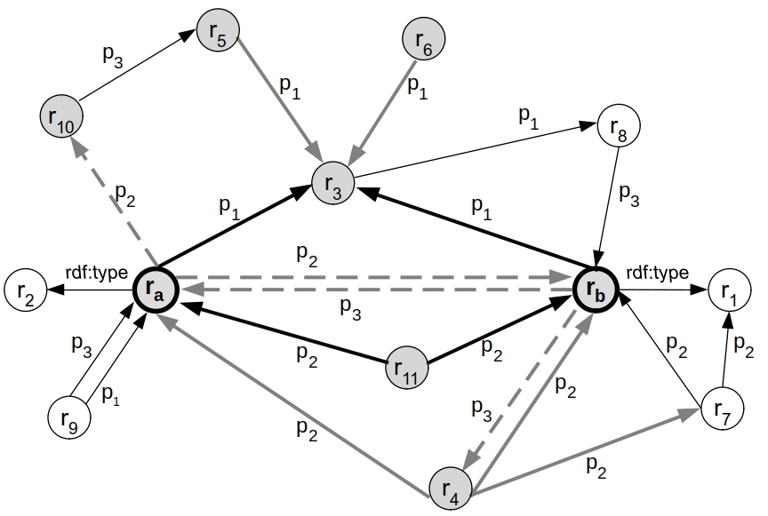
Figure 9: LDSD applied to the running example graph

LDSD_iw. The second measure is the indirect weighted LDSD, indicated as $LDSD_{iw}$. It basically considers all the path patterns in the graph identified by those resources linked to both the compared resources via the same predicate. Let $C_{io}$ and $C_{ii}$ be functions that compute the number of indirect and distinct links between resources, outgoing and incoming respectively, as follows. Given two resources $r_{a}$, $r_{b}$ and a predicate $p_{j}$, $C_{io}(p_{j},r_{a},r_{b})$ = 1 if there exists a resource $r_{n}$ that satisfies both $\langle r_{a},p_{j},r_{n}\rangle$, and $\langle r_{b},p_{j},r_{n}\rangle$, otherwise $C_{io}(p_{j},r_{a},r_{b})$ = 0. Analogously, $C_{ii}(p_{j},r_{a},r_{b})$ = 1 if there exists a resource $r_{n}$ that satisfies both $\langle r_{n},p_{j},r_{a}\rangle$, and $\langle r_{n},p_{j},r_{b}\rangle$, otherwise $C_{ii}(p_{j},r_{a},r_{b})$ = 0. Furthermore, let $C_{io}(p_{j},r_{a})$ and $C_{ii}(p_{j},r_{a})$ be the total number of resources indirectly linked to $r_{a}$ via the predicate $p_{j}$, outgoing and incoming respectively. Hence, given the resources $r_{a}$ and $r_{b}$, $LDSD_{iw}(r_{a},r_{b})$ addresses the indirect incoming and outgoing links between the resources, and is defined according to Eq. 6.

$$LDSD_{iw}(r_{a},r_{b})=\frac{1}{1+\sum_{p_{j}\in U}\frac{C_{io}(p_{j},r_{a},r_{b})}{1+log(C_{io}(p_{j},r_{a}))}+\sum_{p_{j}\in V}\frac{C_{ii}(p_{j},r_{a},r_{b})}{1+log(C_{ii}(p_{j},r_{a}))}}$$ (6)

where $U\subseteq R$ is the set of the predicates $p_{j}$ in the graph $\mathcal{G}$ such that $C_{io}(p_{j},r_{a},r_{b})=1$, and $V\subseteq R$ is the set of the predicates $p_{j}$ in $\mathcal{G}$ such that $C_{ii}(p_{j},r_{a},r_{b})=1$.

In the example of Figure 3, the resource $r_{3}$, with incoming links labeled with the predicate $p_{1}$ (one outgoing from $r_{a}$ and the other one from $r_{b}$), and both the resources $r_{4}$ and $r_{11}$, with outgoing links labeled with the predicate $p_{2}$ (and incoming to $r_{a}$ and $r_{b}$, accordingly), satisfy the above conditions for $C_{io}(p_{1},r_{a},r_{b})$ and $C_{ii}(p_{2},r_{a},r_{b})$ respectively, therefore $C_{io}(p_{1},r_{a},r_{b})$ = 1 and $C_{ii}(p_{2},r_{a},r_{b})$ = 1. Note that only one resource with indirect incoming links is needed in order to have $C_{ii}(p_{2},r_{a},r_{b})$ = 1, for instance $r_{11}$. For this reason, in order to highlight this point, in Figure 9, besides the indirect outgoing links related to $r_{3}$, only the indirect incoming links related to $r_{11}$ have been drawn in bold.

LDSD_cw. Finally, the author proposes the combined weighted $LDSD$ distance between the resources $r_{a}$ and $r_{b}$, indicated as $LDSD_{cw}(r_{a},r_{b})$, that is a combination of the previous distances, the direct and indirect ones, defined as follows:

$$LDSD_{cw}(r_{a},r_{b})=\frac{1}{1+f_{1}+f_{2}}\\$$ (7)

where:

$f_{1}=\sum_{p_{j}\in W}\frac{C_{d}(p_{j},r_{a},r_{b})}{1+log(C_{d}(p_{j},r_{a}))}+\sum_{p_{j}\in Z}\frac{C_{d}(p_{j},r_{b},r_{a})}{1+log(C_{d}(p_{j},r_{b}))}$

$f_{2}=\sum_{p_{j}\in U}\frac{C_{io}(p_{j},r_{a},r_{b})}{1+log(C_{io}(p_{j},r_{a}))}+\sum_{p_{j}\in V}\frac{C_{ii}(p_{j},r_{a},r_{b})}{1+log(C_{ii}(p_{j},r_{a}))}$

and $W\subseteq R$ is the set of the predicates $p_{j}$ in the graph $\mathcal{G}$ such that $C_{d}(p_{j},r_{a},r_{b})=1$, $Z\subseteq R$ is the set of the predicates $p_{j}$ in $\mathcal{G}$ such that $C_{d}(p_{j},r_{b},r_{a})=1$, $U\subseteq R$ is the set of the predicates $p_{j}$ in $\mathcal{G}$ such that $C_{io}(p_{j},r_{a},r_{b})=1$, and $V\subseteq R$ is the set of the predicates $p_{j}$ in $\mathcal{G}$ such that $C_{ii}(p_{j},r_{a},r_{b})=1$.

In our running example, the $LDSD_{cw}$ measure involves all the links and the nodes highlighted in Figure 9. Note that the distance defined according to Eq. 7 is not symmetric. This point is addressed by the measure recalled in the next subsection. According to the results given in [43], the $LDSD_{cw}$ measure performs better than the $LDSD_{dw}$ and the $LDSD_{iw}$ measures.

A.2.2 LDSD with Global Normalization (LDSDGN)

The LDSD with Global Normalization (LDSDGN) measure [44] is an evolution of the approach presented by Passant [43], where the normalization addresses both the compared resources and the global appearances of specific path patterns in the graph. In a previous work [45], the authors claim that, given two resources $r_{a}$ and $r_{b}$, with $r_{a}$ $\neq$ $r_{b}$, a distance measure $d$ should satisfy the following three axioms:

(i) Equal self-distance, i.e., d$(r_{a},r_{a})$ = d$(r_{b},r_{b})=0$.

(ii) Symmetry, i.e., d$(r_{a},r_{b})$ = d$(r_{b},r_{a})$.

(iii) Minimality, i.e., d$(r_{a},r_{a})$ $<$ d$(r_{a},r_{b})$.

Hence, they put in evidence that all the measures introduced by Passant do not satisfy both the axioms (i) and (iii), and this is because the distance between any resource and itself depends on its incoming and outgoing links. Furthermore, the $LDSD_{cw}$ measure does not even satisfy the symmetry axiom because Eq. 7 addresses only the total number of resources indirectly linked to $r_{a}$, whereas the ones linked to $r_{b}$ are not considered. For this reasons, in order to meet the mentioned requirements, in [44] the authors propose a family of $LDSD$ measures satisfying the three axioms above. In particular, in the following, the distances the $LDSD_{\alpha}$, $LDSD_{\beta}$ and $LDSD_{\gamma}$ are recalled.

LDSD_α. Given a graph $\mathcal{G}$, analogously to the notation used by Passant in [43], below $C_{d}(p_{j},r_{a},r_{b})$ = 1 if in the graph there exists a triple $\langle r_{a},p_{j},r_{b}\rangle$, otherwise $C_{d}(p_{j},r_{a},r_{b})$ = 0, and the total number of resources that can be reached from $r_{a}$ by means of the predicate $p_{j}$ is indicated by $C_{d}(p_{j},r_{a})$ (analogously, $C_{d}(p_{j},r_{b})$). Similarly, $C_{io}(p_{j},r_{a})$ and $C_{ii}(p_{j},r_{a})$ are the total number of resources indirectly linked to $r_{a}$ via outgoing and incoming links labeled with the predicate $p_{j}$, respectively. Furthermore, on the basis of the assumption that resources are more related if there is a great number of them linked via a given predicate $p_{k}$, the $C_{io}$ ($C_{ii}$) function defined by Passant has been generalized by using the function $C^{\prime}_{io}$ ($C^{\prime}_{ii}$) as follows: $C^{\prime}_{io}(p_{k},r_{a},r_{b})$ ($C^{\prime}_{ii}(p_{k},r_{a},r_{b})$) computes the total number of resources linked to $r_{a}$ and $r_{b}$ via an outgoing (incoming) predicate $p_{k}$. Therefore, given the resources $r_{a}$, $r_{b}$, the first distance is the $LDSD_{\alpha}(r_{a},r_{b})$ measure defined in Eq. 8.

$$LDSD_{\alpha}(r_{a},r_{b})=\frac{1}{1+f_{1}+f_{2}}\\$$ (8)

where:

$f_{1}=\sum_{p_{j}\in U}\frac{C_{d}(p_{j},r_{a},r_{b})}{1+log(C_{d}(p_{j},r_{a}))}+\sum_{p_{j}\in V}\frac{C_{d}(p_{j},r_{b},r_{a})}{1+log(C_{d}(p_{j},r_{b}))}\\$

$f_{2}=\sum_{p_{j}\in W}\frac{C^{\prime}_{io}(p_{j},r_{a},r_{b})}{1+log(C_{io}(p_{j},r_{a}))}+\sum_{p_{j}\in Z}\frac{C^{\prime}_{ii}(p_{j},r_{a},r_{b})}{1+log(C_{ii}(p_{j},r_{a}))}$

and $U\subseteq R$ is the set of the predicates $p_{j}$ in the graph $\mathcal{G}$ such that $C_{d}(p_{j},r_{a},r_{b})=1$, $V\subseteq R$ is the set of the predicates $p_{j}$ in $\mathcal{G}$ such that $C_{d}(p_{j},r_{b},r_{a})=1$, $W\subseteq R$ is the set of the predicates $p_{j}$ in $\mathcal{G}$ such that $C^{\prime}_{io}(p_{j},r_{a},r_{b})>0$, and $Z\subseteq R$ is the set of the predicates $p_{j}$ in $\mathcal{G}$ such that $C^{\prime}_{ii}(p_{j},r_{a},r_{b})>0$.

In the example of Figure 3, $C^{\prime}_{ii}(p_{2},r_{a},r_{b})$ = 2 since there are two resources, namely $r_{4}$ and $r_{11}$, both with incoming links to $r_{a}$ and $r_{b}$ labeled with the predicate $p_{2}$. In Figure 10 these resources are filled with upward diagonals, and the involved links are highlighted in grey.

Figure 10: LDSDGN applied to the running example graph

LDSD_β. With respect to $LDSD_{\alpha}$, in the $LDSD_{\beta}$ measure the last two addenda at the denominator are modified by addressing the averages between $C_{io}(p_{j},r_{a})$, $C_{io}(p_{j},r_{b})$, and $C_{ii}(p_{j},r_{a})$, $C_{ii}(p_{j},r_{b})$ respectively, in order to achieve symmetry. In particular, given the resources $r_{a}$, and $r_{b}$, $LDSD_{\beta}(r_{a},r_{b})$ is defined according to Eq. 9.

$$LDSD_{\beta}(r_{a},r_{b})=\frac{1}{1+f_{1}+f_{2}}$$ (9)

where:

$f_{1}=\sum_{p_{j}\in U}\frac{C_{d}(p_{j},r_{a},r_{b})}{1+log(C_{d}(p_{j},r_{a}))}+\sum_{p_{j}\in V}\frac{C_{d}(p_{j},r_{b},r_{a})}{1+log(C_{d}(p_{j},r_{b}))}$

$f_{2}=\sum_{p_{j}\in W}\frac{C^{\prime}_{io}(p_{j},r_{a},r_{b})}{1+log(\frac{C_{io}(p_{j},r_{a})+C_{io}(p_{j},r_{b})}{2})}+\sum_{p_{j}\in Z}\frac{C^{\prime}_{ii}(p_{j},r_{a},r_{b})}{1+log(\frac{C_{ii}(p_{j},r_{a})+C_{ii}(p_{j},r_{b})}{2})}$

and $U\subseteq R$ is the set of the predicates $p_{j}$ in the graph $\mathcal{G}$ such that $C_{d}(p_{j},r_{a},r_{b})=1$, $V\subseteq R$ is the set of the predicates $p_{j}$ in $\mathcal{G}$ such that $C_{d}(p_{j},r_{b},r_{a})=1$, $W\subseteq R$ is the set of the predicates $p_{j}$ in $\mathcal{G}$ such that $C^{\prime}_{io}(p_{j},r_{a},r_{b})>0$, and $Z\subseteq R$ is the set of the predicates $p_{j}$ in $\mathcal{G}$ such that $C^{\prime}_{ii}(p_{j},r_{a},r_{b})>0$.

Therefore, in the $LDSD_{\beta}(r_{a},r_{b})$ distance further links are captured by the function $C_{ii}(p_{2},r_{b})$, that are highlighted with dashed grey arrows in Figure 10, with the nodes of the involved resources, $r_{7}$ and $r_{1}$, in grey.

LDSD_γ. In [44] the authors state that all the above recalled measures, including Eq. 7 of Passant, involve a local normalization that takes into account the paths “in the context” of the resources. For this reason, in the mentioned paper, the authors propose a further measure, namely $LDSD_{\gamma}$, relying on a global normalization notion that essentially considers the importance of a path between two resources according to the number of its occurrences in the whole graph $\mathcal{G}$. In the following, let $C_{dp}(p_{j})$ be the global occurrences of the link $p_{j}$ between two resources in $\mathcal{G}$. Furthermore, $C_{io}(p_{k},r_{j},r_{a},r_{b})$ = 1 if there exists a resource $r_{j}$ such that $\langle r_{a},p_{k},r_{j}\rangle$ and $\langle r_{b},p_{k},r_{j}\rangle$, and $C_{ii}(p_{k},r_{j},r_{a},r_{b})$ = 1 if there exists a resource $r_{j}$ such that $\langle r_{j},p_{k},r_{a}\rangle$ and $\langle r_{j},p_{k},r_{b}\rangle$.

The normalizations of $C_{io}(p_{k},r_{j},r_{a},r_{b})$ and $C_{ii}(p_{k},r_{j},r_{a},r_{b})$ are carried out by using the global occurrences $C_{iop}(p_{k},r_{j})$ and $C_{iip}(p_{k},r_{j})$ of $r_{j}$ as follows. $C_{iop}(p_{k},r_{j})$ returns the global occurrences of $r_{j}$ in the undirected paths $[\langle r_{n},p_{k},r_{j}\rangle$, $\langle r_{s},p_{k},r_{j}\rangle$], for any resources $r_{n}$, $r_{s}$ in the graph $\mathcal{G}$ and, analogously, $C_{iip}(p_{k},r_{j})$ computes the global occurrences of $r_{j}$ in the undirected paths $[\langle r_{j},p_{k},r_{n}\rangle$, $\langle r_{j},p_{k},r_{s}\rangle]$, for any resources $r_{n}$, $r_{s}$ in $\mathcal{G}$.

According to the above assumptions, given $r_{a}$ and $r_{b}$, $LDSD_{\gamma}(r_{a},r_{b})$ is defined in Eq. 10.

$$LDSD_{\gamma}(r_{a},r_{b})=\frac{1}{1+f_{1}+f_{2}}$$ (10)

where:

$f_{1}=\sum_{p_{j}\in U}\frac{C_{d}(p_{j},r_{a},r_{b})}{1+log(C_{dp}(p_{j}))}+\sum_{p_{j}\in V}\frac{C_{d}(p_{j},r_{b},r_{a})}{1+log(C_{dp}(p_{j}))}$

$f_{2}=\sum_{(p_{k},r_{j})\in W}\frac{C_{io}(p_{k},r_{j},r_{a},r_{b})}{1+log(C_{iop}(p_{k},r_{j}))}+\sum_{(p_{k},r_{j})\in Z}\frac{C_{ii}(p_{k},r_{j},r_{a},r_{b})}{1+log(C_{iip}(p_{k},r_{j}))}$

and $U\subseteq R$ is the set of the predicates $p_{j}$ in the graph $\mathcal{G}$ such that $C_{d}(p_{j},r_{a},r_{b})=1$, $V\subseteq R$ is the set of the predicates $p_{j}$ in $\mathcal{G}$ such that $C_{d}(p_{j},r_{b},r_{a})=1$, $W\subseteq R\times R$ is the set of the pairs ($p_{k}$, $r_{j}$) such that $C_{io}(p_{k},r_{j},r_{a},r_{b})=1$, and $Z\subseteq R\times R$ is the set of the pairs ($p_{k}$, $r_{j}$) such that $C_{ii}(p_{k},r_{j},r_{a},r_{b})=1$.

For instance, in our running example, assume $k$ = 1, and $j$ = 3. Then, $C_{io}(p_{1},r_{3},r_{a},r_{b})$ is equal to 1 because there exists the resource $r_{3}$, and $\langle r_{a},p_{1},r_{3}\rangle$ and $\langle r_{b},p_{1},r_{3}\rangle$ are triples belonging to the graph. It is normalized according to $C_{iop}(p_{1},r_{3})$, that returns the global occurrences of the resource $r_{3}$ in the graph, identified by the links $\langle r_{5},p_{1},r_{3}\rangle$, $\langle r_{6},p_{1},r_{3}\rangle$, highlighted with long dashed grey arrows in Figure 10.

According to the results presented in [44], $LDSD_{\gamma}$ performs better than the $LDSD_{\alpha}$ and $LDSD_{\beta}$ measures.

A.2.3 Propagated Linked Data Semantic Distance (PLDSD)

The Propagated Linked Data Semantic Distance ($PLDSD$) [4] allows the evaluation of the relatedness of two resources by considering the distance computed according to $LDSD_{cw}$ (see Eq. 7) between the adjacent resources in all the paths linking the compared resources, up to a given length. As a result, with respect to the $LDSD_{cw}$ measure, in this approach additional pairs of resources are considered in the semantic relatedness evaluation. Note that the aforementioned paper focuses on recommendation systems and, in order to face with efficiency problems, the authors reduce the knowledge graph by addressing only the resources identified by the system in the given domain.

Given the resources $r_{a}$ and $r_{b}$ in a knowledge graph $\mathcal{G}$, and $h>0$ that is the maximum length of the paths to be considered, the semantic relatedness $PLDSD_{h}(r_{a},r_{b})$ can be summarized according to Eq. 11:

$$PLDSD_{h}(r_{a},r_{b})=\underset{P\in\mathcal{P}^{h}}{max}\prod_{i=1}^{length(P)}(1-LDSD_{cw}(s_{i},o_{i}))$$ (11)

where:

• $\mathcal{P}^{h}$ is the set of the undirected paths $P$ connecting $r_{a}$ and $r_{b}$ with length less than or equal to $h$.

• $s_{i}$ and $o_{i}$ are the subject and the object, respectively, of the i-th triple in the path $P$.

• $length(P)$ is the length of the path $P$.

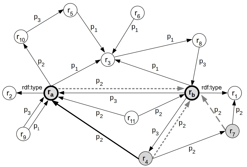
Figure 11: PLDSD applied to the running example graph

According to the above formula, it is possible to see the reason why, with respect to the $LDSD_{cw}$, additional resources are considered in the relatedness evaluation. For instance, consider the resources $r_{a}$ and $r_{b}$ of the running example of Figure 3. In Figure 9 we have seen that the resource $r_{4}$ has been considered in the evaluation of the $LDSD_{cw}(r_{a},r_{b})$ since it has outgoing links towards both $r_{a}$ and $r_{b}$ labeled with the predicate $p_{2}$, but the resource $r_{7}$, for instance, is not involved in the computation. This is not the case of the $PLDSD$ approach, where also $r_{7}$ is addressed. In fact, when considering the link highlighted in bold in Figure 11, corresponding to the triple $\langle r_{4},p_{2},r_{a}\rangle$ of the path [$\langle r_{4},p_{2},r_{a}\rangle$, $\langle r_{4},p_{2},r_{b}\rangle$], the $LDSD_{cw}$ applied to the pair $(r_{4},r_{a})$ (whose resources are indirectly linked via $p_{2}$, as shown by the dashed grey arrows drawn in Figure 11) involves $r_{7}$ since it is indirectly connected to $r_{4}$ via the predicate $p_{2}$, as highlighted by the additional long dashed grey arrow of Figure 11.

A.3 Methods based on triple weights

In this subsection the methods belonging to the third group are described, which require the association of weights with triples in order to evaluate the contributions of the different paths.

A.3.1 Information Content-based Measure (ICM)

The Information Content-based Measure (ICM) requires the evaluation of the weights of the triples belonging to the undirected paths linking the compared resources, up to a given length [53]. Such a weight is computed on the basis of the information content notion recalled below.

Given a random variable $X$ in the set $\{x_{i}\}$, and a probability distribution $Pr(X)$ over $X$, the information content (IC) associated with $X=x_{i}$, i.e., the event that the variable $X$ assumes the value $x_{i}$, is defined in Eq. 12:

$$IC_{Pr(X)}(X=x_{i})=-log(Pr(X=x_{i}))$$ (12)

that can also be written as $IC(x_{i})=-log(Pr(x_{i}))$ for short. Hence, according to the $IC$ notion, specificity is a good proxy for relevance, and the less the probability of an event, the higher its information content.

If the random variable $X$ describes only the predicate of a triple, the weight of the triple depends only on the probability associated with that predicate. Consequently, two triples with the same predicate have the same weight. However, it can be intuitively assessed that two triples having the same predicate, but different objects, in general, convey different amounts of information. This is the case of the following two triples extracted from DBpedia, representing two statements about the resource dbr:Dante_Alighieri:

$\langle$dbr:Dante_Alighieri, rdf:type, dbo:Person$\rangle$

$\langle$dbr:Dante_Alighieri, rdf:type, dbo:Writer$\rangle$

They both have the same predicate, i.e., rdf:type, but since writer is a term more specific than person, the latter represents a more accurate and richer piece of information. For this reason, in order to compute the weight of a triple, both the predicate and the object of the triple are considered, and in the following we assume they are described by the random variables $X$ and $Y$, respectively.

In [53], the authors propose the following three strategies for computing the weight of a triple $t=\langle r_{s},p,r_{o}\rangle$.

Joint Information Content (jointIC). In the case of the jointIC strategy, the weight of the triple $t$, $w_{jointIC}(t)$, is computed according to Eq. 13:

$$w_{jointIC}(t)=IC(p)+IC(r_{o}|p)$$ (13)

where $IC(p)=IC_{Pr(X)}(X=p)$ is the information content associated with probability that the random variable $X$ assumes the value $p$, and $IC(r_{o}|p)=IC_{Pr(Y),Pr(X)}(Y=r_{o}|X=p)$ is the information content associated with the conditional probability that the variable $Y$ assumes the value $r_{o}$, supposing that the variable $X$ assumes the value $p$. Note that, $w_{jointIC}(t)$ is equivalent to the $IC$ of the joint probability $Pr(p,r_{o})$, that is the probability that the variables $X$ and $Y$ assume the values $p$ and $r_{o}$, respectively, and represents the likelihood of randomly selecting, from the considered RDF graph, a triple with $p$ and $r_{o}$ as predicate and object, respectively. Therefore, Eq. 13 can be also written as $w_{jointIC}(t)=IC(p,r_{o})=IC_{Pr(Y),Pr(X)}(X=p,Y=r_{o})$, emphasizing that the triples that contribute to the computation of jointIC are those with predicate $p$ and object $r_{o}$. For instance, if we consider the triple $\langle r_{4},p_{2},r_{a}\rangle$ of the running example, which has been represented with a grey arrow in the graph of Figure 12, the edges relevant to compute jointIC($\langle r_{4},p_{2},r_{a}\rangle$) are the triple itself, and the triple $\langle r_{11},p_{2},r_{a}\rangle$, which has been highlighted with a dashed grey arrow in the same figure, because in the graph there are no other triples with predicates $p_{2}$ and object $r_{a}$.

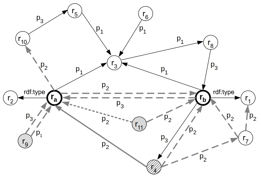
Figure 12: ICM applied to the running example graph

Combined Information Content (combIC). The combIC strategy aims at mitigating the possible penalization of the jointIC measure, in the case of infrequent objects that occur with infrequent predicates, as shown by Eq (14):

$$w_{combIC}(t)=IC(p)+IC(r_{o})$$ (14)

where, with respect to Eq. 13, $IC(r_{o})$ is evaluated independently of the predicate $p$. In fact, the combIC approach is applied while making an independence assumption between the predicate and the object. Consequently, the weight of the triple $t$ results in the sum of the ICs of the predicate and the object. If we consider again the triple $\langle r_{4},p_{2},r_{a}\rangle$ in the graph of Figure 12, according to the combIC strategy, additional triples have to be considered with respect to jointIC, that have been highlighted with long dashed grey arcs in the same figure, i.e., all the triples having either $p_{2}$ as predicate or $r_{a}$ as the object.

Information Content and Pointwise Mutual Information (IC+PMI). According to the IC+PMI strategy, the weight of the triple $t$ can be defined by Eq. 15:

$$w_{IC+PMI}(t)=IC(p)+PMI(p,r_{o})$$ (15)

where:

$$PMI(p,r_{o})=log\frac{Pr(p,r_{o})}{Pr(p)Pr(r_{o})}$$ (16)

In particular, $PMI$ measures the mutual dependence between the two random variables describing the predicate and the object of a triple, and can be seen as a measure of the deviation from independence between the two outcomes. With respect to the previous strategies, by means of the addendum PMI, IC+PMI represents a balance between the assumptions of full dependence (jointIC) and independence (combIC) between predicates and objects. In Eq. 15, the $IC$ of the predicate is summed with $PMI$ in order to bias the weight towards less frequent, and thus more informative, predicates.

Once a strategy has been adopted, given the resources $r_{a}$ and $r_{b}$, and the maximum length $h>0$ of the paths to be considered, the semantic relatedness between $r_{a}$ and $r_{b}$, ICM${}_{h}(r_{a},r_{b})$, is computed according to Eq. 17:

$$\textit{ICM}_{h}(r_{a},r_{b})=\frac{1}{\underset{P\in\mathcal{P}^{h}}{min}\underset{t_{i}\in P}{\sum}(w_{max}-w(t_{i}))}$$ (17)

where:

• $\mathcal{P}^{h}$ is the set of the undirected paths connecting $r_{a}$ and $r_{b}$ with length less than or equal to $h$.

• $t_{i}$ is the i-th triple in the path $P$ of the set $\mathcal{P}^{h}$.

• $w(t)$ is the weight of the triple $t$, and $w_{max}$ is the maximum weight a triple in the graph can assume, according to one of the above three strategies.

In the case $r_{a}\equiv r_{b}$ the semantic relatedness between the resources is assumed to be equal to $1$. On the basis of the results of the experimentation presented in [53], the measure obtained according to combIC outperforms the other two.

A.3.2 REWOrD

According to [46], the REWOrD method is based on the notion of informativeness of predicates, in line with the Term Frequency-Inverse Document Frequency (TF-IDF) approach. TF-IDF is generally used in information retrieval to evaluate the relevance of a term w in a document d belonging to a collection D of documents. The Term Frequency (TF) of the term w with respect to the document d represents the number of times w appears in d divided by the total number of terms in d. The Inverse Document Frequency (IDF) represents the logarithm of the ratio between the total number of documents in D and the number of documents containing the term w.

In the case of an RDF graph, say $\mathcal{G}$, TF-IDF deals with predicates instead of terms, and resources and triples instead of documents, therefore becomes Predicate Frequency-Inverse Triple Frequency (PF-ITF). As mentioned in Section 5.3, we need to distinguish between incoming and outgoing Predicate Frequency (PF). In particular, the incoming PF of a predicate p with respect to a resource r, say $PF_{i}^{r}(p)$, resembles the TF as defined in Eq. 18:

$$PF_{i}^{r}(p)=\frac{|T_{i}^{r}(p)|}{|T^{r}|}$$ (18)

where:

• $|T_{i}^{r}(p)|=|\{\langle?r_{i},p,r\rangle\}|$ is the number of triples having predicate p and object r, i.e., incoming to $r$.

• $|T^{r}|=|\{\langle r,?p_{i},?r_{k}\rangle\}\cup\{\langle?r_{h},?p_{j},r\rangle\}|$ is the number of triples where the resource $r$ appears.

The Inverse Triple Frequency (ITF) resembles the IDF as defined in Eq. 19:

$$ITF(p)=log\frac{|\mathcal{G}|}{|T(p)|}$$ (19)

where:

• $|\mathcal{G}|=|\{\langle?r_{i},?p_{j},?r_{h}\rangle\}|$ is the total number of triples in the graph $\mathcal{G}$.

• $|T(p)|=|\{\langle?r_{i},p,?r_{j}\rangle\}|$ is the number of triples with $p$ as predicate.

Finally, the incoming PF-ITF of the predicate $p$ with respect to the resource $r$, PF-$ITF_{i}^{r}$(p), is defined in Eq. 20:

$$\textit{PF-}ITF_{i}^{r}(p)=PF_{i}^{r}(p)\cdot ITF(p)$$ (20)

and stands for the informativeness of the incoming predicate $p$ with respect to $r$. Analogously, the informativeness of the outgoing predicate $p$ with respect to $r$ is indicated as PF-$ITF_{o}^{r}$(p). For example, consider the resource $r_{a}$ and the predicate $p_{2}$ in the knowledge graph of Figure 3. We have $PF_{i}^{r_{a}}(p_{2})=\frac{2}{9}=0.22$, since the number of triples with predicate $p_{2}$ and object $r_{a}$ is $2$, and the number of triples where $r_{a}$ appears is $9$. Furthermore, $ITF(p_{2})=log(\frac{22}{9})=0.39$, since the total number of triples in the graph is $22$, and the triples with predicate $p_{2}$ are $9$. Therefore, $\textit{PF-}ITF_{i}^{r_{a}}(p_{2})$, i.e., the informativeness of the incoming predicate $p_{2}$ with respect to $r_{a}$, is equal to $0.22\cdot 0.39=0.08$.

The relatedness space of the resource $r$, say $RS(r)$, is the vector of weighted predicates (either incoming or outgoing), where weights are the predicates’ informativeness with respect to $r$. When addressing semantic relatedness between resources, their relatedness spaces can be enriched with the informativeness of the predicates occurring in the most informative path (mip) linking them. The mip is the path with the greatest informativeness, among those connecting the resources, up to a given length. Note that, the method considers undirected paths. Given an undirected path P_n of length n, the informativeness of P_n is the sum of the informativeness of the sub-paths of length 1, i.e., the single triples, divided by $n$, as defined according to Eq. 21:

$$I({P_{n}})=(I({t_{1})}+I({t_{2})}+...+I({t_{n}}))/n$$ (21)

where, for $i$ = $1$ …$n$:

$I({t_{i})}=I(\langle r_{i},p_{i},r_{i+1}\rangle)=(\textit{PF-}ITF_{o}^{r_{i}}(p_{i})+\textit{PF-}ITF_{i}^{r_{i+1}}(p_{i}))/2$, and $\langle r_{i}$, $p_{i}$, $r_{i+1}\rangle$ is the i-th triple of the path $P_{n}$.

The method proposes five strategies for computing the relatedness between two resources $r_{a}$ and $r_{b}$, referred to as reword_incoming, reword_outgoing, reword_average, reword_mip, and reword.

According to reword_incoming, the relatedness spaces for $r_{a}$ and $r_{b}$ are built by considering only the incoming predicates to $r_{a}$ and $r_{b}$, respectively.

Figure 13: REWOrD applied to the running example graph

For instance, consider Figure 13, where the incoming predicates to $r_{a}$ and $r_{b}$ are represented with dashed and long dashed grey arrows, respectively. On the basis of this strategy, the relatedness spaces of $r_{a}$, and $r_{b}$ are:

$RS(r_{a})=[$ $(p_{1},$ PF-ITF${}_{i}^{r_{a}}(p_{1})),$ $(p_{2},$ PF-ITF${}_{i}^{r_{a}}(p_{2})),$ $(p_{3},$ PF-ITF${}_{i}^{r_{a}}(p_{3}))$ $]$
$RS(r_{b})=[$ $(p_{2},$ PF-ITF${}_{i}^{r_{b}}(p_{2})),$ $(p_{3},$ PF-ITF${}_{i}^{r_{b}}(p_{3}))$ $]$

each containing the corresponding resource’s incoming predicates, associated with their informativeness. Analogously, in the case of the reword_outgoing, only the outgoing predicates from $r_{a}$ and $r_{b}$ are considered. The reword_average performs the arithmetic mean between the informativeness computed according to the reword_incoming and reword_outgoing strategies. In the case of reword_mip, the relatedness between $r_{a}$ and $r_{b}$ is evaluated by relying on the informativeness of the mip between the resources. Finally, according to the reword strategy, the relatedness spaces of $r_{a}$ and $r_{b}$ as defined in the case of the reword_incoming approach are considered, both enriched with the informativeness of the predicates in the mip. In particular, for each triple $\langle r_{i},p_{j},r_{k}\rangle$ in the mip, the predicate $p_{j}$, and the related informativeness, is added to both the relatedness spaces of $r_{a}$ and $r_{b}$ and, if $p_{j}$ is already present in one or both the relatedness spaces, its informativeness will increase the existing ones. For example consider Figure 13, where we assume that the mip connecting $r_{a}$ and $r_{b}$ is the undirected path composed of the triples $\langle r_{a},p_{1},r_{3}\rangle$ and $\langle r_{b},p_{1},r_{3}\rangle$, highlighted in bold grey. According to the reword strategy, the resulting relatedness spaces become:

$RS(r_{a})=[$ $(p_{1},$ PF-ITF${}_{i}^{r_{a}}(p_{1})$ + $I(\langle r_{a}$, $p_{1}$, $r_{3}\rangle$) + $I(\langle r_{b}$, $p_{1}$, $r_{3}\rangle$)),
$(p_{2},$ PF-ITF${}_{i}^{r_{a}}(p_{2})),$ $(p_{3},$ PF-ITF${}_{i}^{r_{a}}(p_{3}))$ $]$

$RS(r_{b})=[$ $(p_{1},$ $I(\langle r_{a}$, $p_{1}$, $r_{3}\rangle$) + $I(\langle r_{b}$, $p_{1}$, $r_{3}\rangle$)),
$(p_{2},$ PF-ITF${}_{i}^{r_{b}}(p_{2})),$ $(p_{3},$ PF-ITF${}_{i}^{r_{b}}(p_{3}))$ $]$

where the informativeness of both the triples of the mip have been added to the informativeness of the already existing predicate $p_{1}$ in the relatedness space of $RS(r_{a})$, whereas a further element with the same informativeness has been added to the relatedness space of $r_{b}$ since the predicate $p_{1}$ is not defined in $RS(r_{b})$.

Finally, the relatedness between $r_{a}$ and $r_{b}$ is computed as the cosine between the two relatedness spaces. In accordance with the results of the experimentation given in [46], the reword strategy outperforms the others.

A.3.3 Exclusivity-based Measure (ExclM)

As mentioned in Section 5.3, the Exclusivity-based Measure (ExclM) computes the weight of a triple on the basis of the notion of exclusivity [27].

Given a triple $t=\langle r_{i},p,r_{j}\rangle$, the exclusivity of $t$ is formally defined according to Eq. 22:

$$exclusivity(\langle r_{i},p,r_{j}\rangle)=\frac{1}{|\{\langle r_{i},p,?r_{x}\rangle\}|+|\{\langle?r_{y},p,r_{j}\rangle\}|-1}$$ (22)

where:

• $\{\langle r_{i},p,?r_{x}\rangle\}$ is the set of triples with subject $r_{i}$ and predicate $p$.

• $\{\langle?r_{y},p,r_{j}\rangle\}$ is the set of triples with object $r_{j}$ and predicate $p$.

Since the triple $\langle r_{i},p,r_{j}\rangle$ belongs to both the above sets, 1 is subtracted at the denominator to avoid that triple being counted twice.

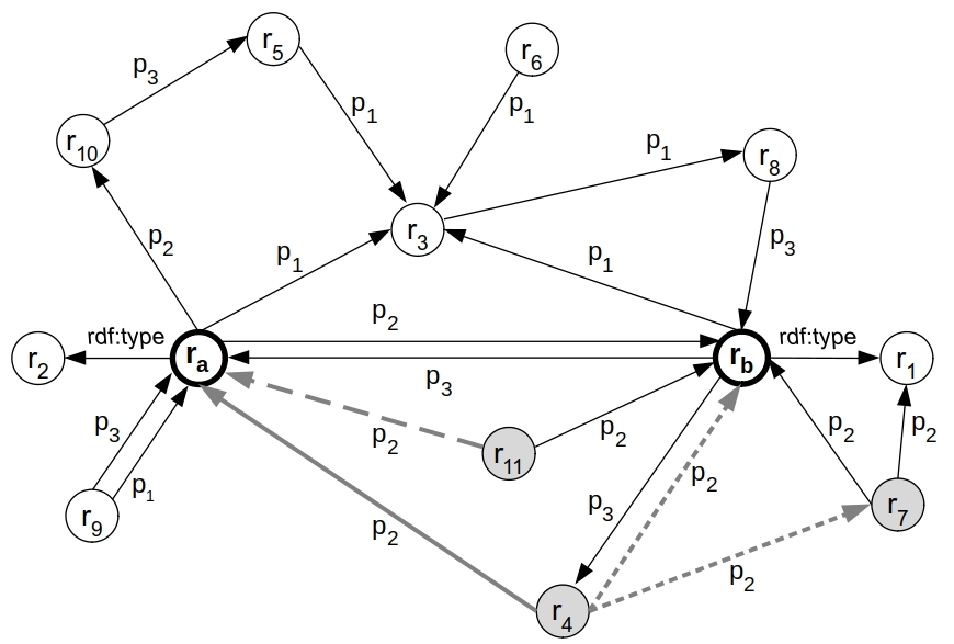
Figure 14: ExclM applied to the running example graph

Consider in our running example the triple $t=\langle r_{4},p_{2},r_{a}\rangle$, highlighted with a bold grey arrow in Figure 14. In addition to $t$, the triples having predicate $p_{2}$ and subject $r_{4}$ are 2, whose edges are highlighted with dashed grey arrows in the same figure, therefore they are 3 in total. The triples having predicate $p_{2}$ and object $r_{a}$ are 2, and are the triple $t$, and the triple drawn with a long dashed grey arrow. Therefore, $exclusivity(t)=1/(3+2-1)=1/4=0.25$.

Based on the exclusivity function, a path weighting function is introduced. This approach assumes that links in an RDF graph can be traversed in both directions and, for this reason, undirected paths are considered.

Let $P=[t_{1},...,t_{n}]$ be a sequence of triples representing an undirected path, the weight of $P$, $w(P)$, is defined in Eq. 23.

$$w(P)=\frac{1}{\sum_{1}^{n}\frac{1}{exclusivity(t_{i})}}$$ (23)

Finally, given two resources $r_{a}$ and $r_{b}$, two integers $h$ and $k$ greater than $0$, and a constant $\alpha$, the relatedness $Eexcl_{h,k}^{\alpha}(r_{a},r_{b})$ is defined in Eq. 24:

$$Excl_{h,k}^{\alpha}(r_{a},r_{b})=\sum_{P_{i}\in\mathcal{P}^{h}_{k}}\alpha^{length(P_{i})}\cdot w(P_{i})$$ (24)

where:

• $\mathcal{P}^{h}_{k}$ is the set of the top-k undirected paths with length less than or equal to $h$, among the ones connecting $r_{a}$ and $r_{b}$, i.e., the $k$ paths with the greatest weights.

• $0<\alpha\leq 1$ is a constant raised to the power of the length of the path $P_{i}$, length($P_{i}$), in $\mathcal{P}^{h}_{k}$ that inspired by the Katz’s centrality measure, and aims at penalizing longer paths.

• $w(P_{i})$ is the weight of the path $P_{i}$ defined above.

In [27], the authors consider $k\in\{1,5,10\}$, and $\alpha\in\{0.25,0.5,0.75,1\}$ in their experiment, and show that $k=5$ and $\alpha=0.25$ lead to better results.

A.3.4 $ASRMP_{m}$

As mentioned in Section 5.3, the $ASRMP_{m}$ family of relatedness measures originates from the previous proposal of the authors named Weighted Semantic Relatedness Measure ($WSRM$) [12]. Therefore, let us start by recalling the $WSRM$ measure and, successively, the $ASRMP_{m}$ family.

Consider an RDF graph $\mathcal{G}$, and the set $R$ of all the resources labeling such a graph, as defined in Section 4. Given two resources $r_{a}$, $r_{b}$ $\in$ $R$, the $WSRM(r_{a},r_{b})$ between $r_{a}$, $r_{b}$ is defined in Eq. 25:

$$WSRM(r_{a},r_{b})=\frac{|\{p|\langle r_{a},p,r_{b}\rangle\in\mathcal{G}\}|}{\sum_{r^{\prime}\in R}|\{p^{\prime}|\langle r_{a},p^{\prime},r^{\prime}\rangle\in\mathcal{G}\}|}$$ (25)

where for any set S, $|S|$ is the cardinality of S. According to the mentioned paper, the authors propose different strategies to evaluate semantic relatedness.

ASRMP${}_{m}^{a}$. We start by recalling the $ASRMP_{m}^{a}$ measure that considers all the paths between the compared resources of length equal to $m$. In particular, given two resources $r_{i}$, $r_{j}$, $ASRMP_{m}^{a}(r_{i},r_{j})$ is defined as shown in Eq. 26:

$$ASRMP_{m}^{a}(r_{i},r_{j})=\oplus_{q\in\mathcal{P}^{m}}\otimes_{k=1}^{m}WSRM(r_{k},r_{k+1})$$ (26)

where:

• $\mathcal{P}^{m}$ is the set of the directed paths between $r_{i}$ and $r_{j}$ with length equal to $m$.

• $r_{k}$ is the $k^{th}$ resource of the path $q$ (therefore $r_{1}$ = $r_{i}$, and $r_{m+1}$ = $r_{j}$).

• $\otimes$ and $\oplus$ are the t-norm and the related s-norm aggregators, respectively, the former for the edges of a given path, and the latter for different paths of length $m$.

Note that, among the different aggregators available in the literature, the fuzzy logic operators t-norm for $\otimes$, and the s-norm for $\oplus$, have been chosen by the authors in order to ensure transitivity. In particular, according to the experimental results defined in the literature, the Hamacher t-norm operator recalled in Eq. 27:

$$T_{H,0}(x,y)=\frac{xy}{x+y-xy}$$ (27)

with its associated s-norm, has been selected by the authors as the best aggregator.

ASRMP${}_{m}^{b}$. Given the resources $r_{i}$, $r_{j}$, the second measure proposed by the authors is $ASRMP_{m}^{b}(r_{i},r_{j})$ that, with respect the previous one, aggregates all the paths of length less than or equal to $m$, as defined in Eq. 28.

$$ASRMP_{m}^{b}(r_{i},r_{j})=\oplus_{q\in\mathcal{P}^{m}}\otimes_{k=1}^{|q|}WSRM(r_{k},r_{k+1})$$ (28)

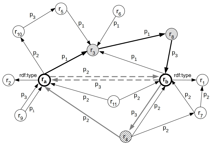
Figure 15: ASRMP_m applied to the running example graph

where $\mathcal{P}^{m}$ is the set of the directed paths between $r_{i}$ and $r_{j}$ of length less than or equal to $m$. However, the authors state that direct links should represent stronger relations, whereas indirect ones should account for weaker relations and, therefore, the longer the path, the weaker the relation. For this reason, they propose a third measure, recalled below.

ASRMP${}_{m}^{c}$. According to $ASRMP_{m}^{c}(r_{i},r_{j})$, paths are weighted on the basis of their length $n$, $n$ = $1$..$m$, as shown in Eq. 29:

$$ASRMP_{m}^{c}(r_{i},r_{j})=\sum_{n=1}^{m}\sum_{q\in\mathcal{P}^{n}}w_{n}\otimes_{k=1}^{n}WSRM(r_{k},r_{k+1})$$ (29)

where:

• $\mathcal{P}^{n}$ is the set of the directed paths between $r_{i}$ and $r_{j}$ with length equal to $n$.

• $w_{n}$ is a length-dependent weight, approximately corresponding to the percentage of paths of length n.

Finally, in order to achieve symmetry, the three strategies above are reformulated according to the $\psi_{m}^{x}(r_{i},r_{j})$ relatedness measure defined in Eq. 30.

$$\psi_{m}^{x}(r_{i},r_{j})=\frac{1}{2}(ASRMP_{m}^{x}(r_{i},r_{j})+ASRMP_{m}^{x}(r_{j},r_{i})),\,\,\,\,\,x\in\{a,b,c\}$$ (30)

Consider again the resources $r_{a}$, $r_{b}$ of the running example of Figure 3, and assume $m$ = $3$. In the case of the measure $\psi_{3}^{a}(r_{a},r_{b})$, the paths of length $3$ are considered that are represented by the only path [$\langle r_{a},p_{1},r_{3}\rangle$, $\langle r_{3},p_{1},r_{8}\rangle$, $\langle r_{8},p_{3},r_{b}\rangle$], that is highlighted with bold arrows in Figure 15. Whereas, in the case of the measure $\psi_{3}^{b}(r_{a},r_{b})$, besides the previous one, also the paths with lengths less than $3$ are addressed, that are the one of length $2$, i.e., [$\langle r_{b},p_{3},r_{4}\rangle$, $\langle r_{4},p_{2},r_{a}\rangle$], highlighted with bold grey arrows in Figure 15, and the ones of length $1$, i.e., [$\langle r_{a},p_{2},r_{b}\rangle$], and [$\langle r_{b},p_{3},r_{a}\rangle$], represented with long dashed grey arrows in the same figure.

Among the proposed strategies, the authors state that $ASRMP_{m}^{a}$ is the best one, in particular for Entity Linking tasks.

A.3.5 Proximity-based Method (ProxM)

According to the Proximity-based Method (ProxM) [32], given the resources $r_{a}$ and $r_{b}$, and an integer $h$ standing for the maximum length of a path, the relatedness (proximity) between them, $prox_{h}(r_{a},r_{b})$, is defined in Eq. 31:

$$prox_{h}(r_{a},r_{b})=\frac{1}{\Omega(\mathcal{G})}\sum_{n=1}^{h}\frac{1}{2^{n}\Delta(\mathcal{G})^{n}}\sum_{P\in\mathcal{P}^{n}}\sum_{t_{i}\in P}w(p_{i})$$ (31)

where:

• $\Omega(\mathcal{G})$ is the maximum weight a predicate in $\mathcal{G}$ can be associated with.

• $\Delta(\mathcal{G})$ is the maximum outdegree of the nodes in $\mathcal{G}$.

• $\mathcal{P}^{n}$ is the set of the undirected paths connecting $r_{a}$ and $r_{b}$ with length $1\leq n\leq h$.

• $w(p_{i})$ is a function that associates the predicate $p_{i}$ of the triple $t_{i}$ with a weight, which is manually assigned in the experiment provided in [32].

Finally, if $r_{a}\equiv r_{b}$, $prox_{h}(r_{a},r_{b})$ is assumed to be equal to 1.

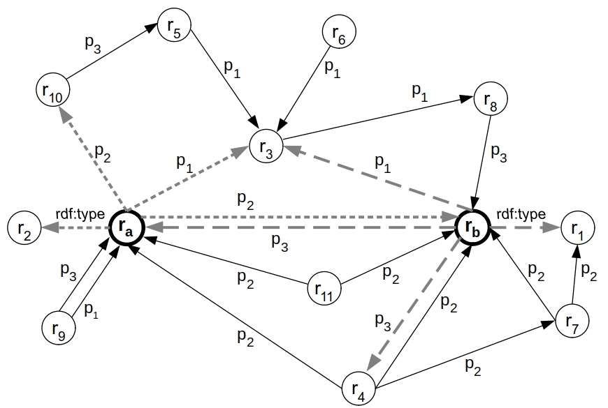
Figure 16: ProxM applied to the running example graph

For instance, consider the graph of our running example. We have $\Delta(\mathcal{G})=4$ since 4 is the maximum outdegree of the nodes of the graph. In particular, both $r_{a}$ and $r_{b}$ have outdegree equal to 4 (see the dashed grey and long dashed grey lines, respectively, in Figure 16). Furthermore, suppose that the predicates $p_{1}$, $p_{2}$, $p_{3}$, $p_{4}$, and rdf:type have been associated with the weights $0.5$, $0.3$, $0.2$, $0.7$, and $0.6$, respectively, then $\Omega(\mathcal{G})=0.7$ that is the maximum among the predicates weights.

References

- Agirre et al. [2009] Eneko Agirre, Enrique Alfonseca, Keith Hall, Jana Kravalova, Marius Paşca, and Aitor Soroa. A study on similarity and relatedness using distributional and wordnet-based approaches. In Proceedings of Human Language Technologies: The 2009 Annual Conference of the North American Chapter of the Association for Computational Linguistics, NAACL ’09, pages 19–27, Stroudsburg, PA, USA, 2009. Association for Computational Linguistics. ISBN 978-1-932432-41-1.
- Ahmed et al. [2021] Rafeeq Ahmed, Pradeep Kumar Singh, and Tanvir Ahmad. Novel semantic relatedness computation for multi-domain unstructured data. EAI Endorsed Trans. Energy Web, 8(31):e5, 2021.
- Aizawa [2003] Akiko Aizawa. An information-theoretic perspective of tf–idf measures. Information Processing & Management, 39(1):45–65, 2003.
- Alfarhood et al. [2017] Sultan Alfarhood, Kevin Labille, and Susan Gauch. PLDSD: Propagated Linked Data Semantic Distance. In IEEE 26th Int. Conference on Enabling Technologies: Infrastructure for Collaborative Enterprises, WETICE ’17, pages 278–283, 2017.
- AlMousa et al. [2021] Mohannad AlMousa, Rachid Benlamri, and Richard Khoury. Exploiting non-taxonomic relations for measuring semantic similarity and relatedness in wordnet. Knowl. Based Syst., 212:106565, Jan 2021. ISSN 0950-7051.
- Carpineto et al. [2009] Claudio Carpineto, Stanislaw Osiński, Giovanni Romano, and Dawid Weiss. A survey of web clustering engines. ACM Comput. Surv., 41(3), 2009. ISSN 0360-0300.
- Chandrasekaran and Mago [2021] Dhivya Chandrasekaran and Vijay Mago. Evolution of Semantic Similarity - A Survey. ACM Comput. Surv., 54(2), 2021. ISSN 0360-0300.
- Chatzakis et al. [2021] Manos Chatzakis, Michalis Mountantonakis, and Yannis Tzitzikas. RDFsim: Similarity-Based Browsing over DBpedia Using Embeddings. Inf., 12:440, 10 2021.
- Cilibrasi and Vitanyi [2007] Rudi Cilibrasi and Paul M.B. Vitanyi. The google similarity distance. IEEE Trans. Knowl. Data Eng., 19(3):370–383, 2007.
- Djenouri et al. [2021] Youcef Djenouri, Hiba Belhadi, Karima Akli-Astouati, Alberto Cano, and Jerry Chun-Wei Lin. An ontology matching approach for semantic modeling: A case study in smart cities. Comput. Intell., pages 1–27, 2021.
- Dougnon et al. [2016] Raïssa Yapan Dougnon, Philippe Fournier-Viger, Jerry Chun-Wei Lin, and Roger Nkambou. Inferring social network user profiles using a partial social graph. J. Intell. Inf. Syst., 47(2):313–344, 2016.
- El Vaigh et al. [2019] Cheikh Brahim El Vaigh, François Goasdoué, Guillaume Gravier, and Pascale Sébillot. Using knowledge base semantics in context-aware entity linking. In Proceedings of the ACM Symposium on Document Engineering 2019, DocEng ’19, New York, NY, USA, 2019. Association for Computing Machinery. ISBN 9781450368872.
- El Vaigh et al. [2020] Cheikh Brahim El Vaigh, François Goasdoué, Guillaume Gravier, and Pascale Sébillot. A novel path-based entity relatedness measure for efficient collective entity linking. In Jeff Z. Pan, Valentina Tamma, Claudia d’Amato, Krzysztof Janowicz, Bo Fu, Axel Polleres, Oshani Seneviratne, and Lalana Kagal, editors, The Semantic Web – ISWC 2020, pages 164–182, Cham, 2020. Springer International Publishing. ISBN 978-3-030-62419-4.
- Formica [2006] Anna Formica. Ontology-based concept similarity in Formal Concept Analysis. Inf. Sci., 176(18):2624–2641, 2006. ISSN 0020-0255.
- Formica [2019] Anna Formica. Similarity reasoning in formal concept analysis: from one- to many-valued contexts. Knowl. Inf. Syst., 60(2):715–739, 2019.
- Formica and Taglino [2021] Anna Formica and Francesco Taglino. An enriched information-theoretic definition of semantic similarity in a taxonomy. IEEE Access, 9:100583–100593, 2021.
- Formica et al. [2008] Anna Formica, Michele Missikoff, Elaheh Pourabbas, and Francesco Taglino. Weighted ontology for semantic search. In Robert Meersman and Zahir Tari, editors, On the Move to Meaningful Internet Systems: OTM 2008, pages 1289–1303, Berlin, Heidelberg, 2008. Springer Berlin Heidelberg. ISBN 978-3-540-88873-4.
- Formica et al. [2013] Anna Formica, Michele Missikoff, Elaheh Pourabbas, and Francesco Taglino. Semantic search for matching user requests with profiled enterprises. Comput. Ind., 64(3):191–202, 2013.
- Fournier-Viger et al. [2020] Philippe Fournier-Viger, Ganghuan He, Chao Cheng, Jiaxuan Li, Min Zhou, Jerry Chun-Wei Lin, and Unil Yun. A survey of pattern mining in dynamic graphs. WIREs Data Mining and Knowledge Discovery, 10(6):e1372, 2020.
- Freitas et al. [2013] André Freitas, João Gabriel Oliveira, Seán O’Riain, João C.P. da Silva, and Edward Curry. Querying linked data graphs using semantic relatedness: A vocabulary independent approach. Data Knowl. Eng., 88:126–141, 2013. ISSN 0169-023X.
- Gracia and Mena [2008] Jorge Gracia and Eduardo Mena. Web-based measure of semantic relatedness. In Proceedings of the 9th International Conference on Web Information Systems Engineering, WISE ’08, page 136–150, Berlin, Heidelberg, 2008. Springer-Verlag. ISBN 9783540854807.
- Hadj Taieb et al. [2020] Mohamed Ali Hadj Taieb, Torsten Zesch, and Mohamed Ben Aouicha. A survey of semantic relatedness evaluation datasets and procedures. Artif. Intell. Rev., 53(6):4407–4448, 2020.
- Harari and Katz [2022] Asaf Harari and Gilad Katz. Automatic features generation and selection from external sources: A DBpedia use case. Inf. Sci., 582:398–414, 2022. ISSN 0020-0255.
- Hecht et al. [2012] Brent Hecht, Samuel H. Carton, Mahmood Quaderi, Johannes Schöning, Martin Raubal, Darren Gergle, and Doug Downey. Explanatory semantic relatedness and explicit spatialization for exploratory search. In Proceedings of the 35th International ACM SIGIR Conference on Research and Development in Information Retrieval, SIGIR ’12, page 415–424, New York, NY, USA, 2012. Association for Computing Machinery. ISBN 9781450314725.
- Hoffart et al. [2012] Johannes Hoffart, Stephan Seufert, Dat Ba Nguyen, Martin Theobald, and Gerhard Weikum. Kore: Keyphrase overlap relatedness for entity disambiguation. In Proceedings of the 21st ACM International Conference on Information and Knowledge Management, CIKM ’12, page 545–554, New York, NY, USA, 2012. Association for Computing Machinery. ISBN 9781450311564.
- Huang et al. [2021] Taicheng Huang, Zonglei Zhen, and Jia Liu. Semantic Relatedness Emerges in Deep Convolutional Neural Networks Designed for Object Recognition. Frontiers Comput. Neurosci., 15:625804, 2021.
- Hulpuş et al. [2015] Ioana Hulpuş, Narumol Prangnawarat, and Conor Hayes. Path-Based Semantic Relatedness on Linked Data and Its Use to Word and Entity Disambiguation, pages 442–457. Springer International Publishing, Cham, 2015.
- Hussain et al. [2020] Muhammad Jawad Hussain, Shahbaz Hassan Wasti, Guangjian Huang, Lina Wei, Yuncheng Jiang, and Yong Tang. An approach for measuring semantic similarity between wikipedia concepts using multiple inheritances. Inf. Process. Manag., 57(3):102188, 2020. ISSN 0306-4573.
- Jaccard [1912] Paul Jaccard. The distribution of the flora in the alpine zone.1. New Phytol., 11(2):37–50, 1912. ISSN 1469-8137.
- Kacmajor and Kelleher [2020] M. Kacmajor and J.D. Kelleher. Capturing and measuring thematic relatedness. Lang. Resour. Eval. 54, pages 645–682, 2020.
- Kirkpatrick et al. [2022] Anna Kirkpatrick, Chidozie Onyeze, David Kartchner, Stephen Allegri, Davi Nakajima An, Kevin McCoy, Evie Davalbhakta, and Cassie S. Mitchell. Optimizations for Computing Relatedness in Biomedical Heterogeneous Information Networks: SemNet 2.0. Big Data Cogn. Comput., 6(1):27, 2022.
- Leal [2013] José Paulo Leal. Using proximity to compute semantic relatedness in RDF graphs. Comput. Sci. Inf. Syst., 10(4):1727–1746, 2013.
- Lee et al. [2020] Yang‐Yin Lee, Hao Ke, Ting‐Yu Yen, Hen‐Hsen Huang, and Hsin‐Hsi Chen. Combining and learning word embedding with wordnet for semantic relatedness and similarity measurement. J. Assoc. Inf. Sci. Technol., 71:657–670, 2020.
- Li et al. [2020] Fei Li, Lejian Liao, Lanfang Zhang, Zhu Xinhua, Zhang Bo, and Zheng Wang. An efficient approach for measuring semantic similarity combining wordnet and wikipedia. IEEE Access, 8:184318–184338, 2020.
- Li et al. [2021] Xiaotao Li, Shujuan You, and Wai Chen. Enhancing Accuracy of Semantic Relatedness Measurement by Word Single-Meaning Embeddings. IEEE Access, 9:117424–117433, 2021.
- Lin [1998] Dekang Lin. An information-theoretic definition of similarity. In In Proceedings of the Int. Conf. on Machine Learning, Madison, Wisconsin, USA, Morgan Kaufmann, pages 296–304, 1998.
- Miller and Charles [1991] George A. Miller and Walter G. Charles. Contextual Correlates of Semantic Similarity. Language & Cognitive Processes, 6(1):1–28, 1991. ISSN 01690965.
- Mohamed and Oussalah [2020] Muhidin A. Mohamed and Mourad Oussalah. A hybrid approach for paraphrase identification based on knowledge-enriched semantic heuristics. Lang. Resour. Eval., 54(2):457–485, 2020.
- Natarajan et al. [2022] Senthilselvan Natarajan, Subramaniyaswamy Vairavasundaram, Ketan Kotecha, V. Indragandhi, Saravanan Palani, Jatinderkumar R. Saini, and Logesh Ravi. CD-SemMF: Cross-Domain Semantic Relatedness Based Matrix Factorization Model Enabled With Linked Open Data for User Cold Start Issue. IEEE Access, 10:52955–52970, 2022.
- Nelson et al. [2004] Douglas L. Nelson, Cathy L. McEvoy, and Thomas A. Schreiber. The university of south florida free association, rhyme, and word fragment norms. Behav. Res. Meth. Instrum. Comput., 36(3):402–407, 2004. ISSN 1532-5970.
- Nikzad–Khasmakhi et al. [2019] Narjes Nikzad–Khasmakhi, Mohammadali Balafar, and Reza Feizi–Derakhshi. The state-of-the-art in expert recommendation systems. Eng. Appl. Artif. Intell., 82:126–147, 2019. ISSN 0952-1976.
- Oliveira et al. [2021] Italo L. Oliveira, Renato Fileto, René Speck, Luís P.F. Garcia, Diego Moussallem, and Jens Lehmann. Towards holistic entity linking: Survey and directions. Inf. Syst., 95:101624, 2021. ISSN 0306-4379.
- Passant [2010] Alexandre Passant. Measuring semantic distance on linking data and using it for resources recommendations. In AAAI Spring Symposium: Linked Data Meets Artificial Intelligence, 2010.
- Piao and Breslin [2016] Guangyuan Piao and John G. Breslin. Measuring semantic distance for linked open data-enabled recommender systems. In Proceedings of the 31st Annual ACM Symposium on Applied Computing, SAC ’16, pages 315–320, New York, NY, USA, 2016. ACM. ISBN 978-1-4503-3739-7.
- Piao et al. [2015] Guangyuan Piao, Safina Showkat Ara, and John G. Breslin. Computing the semantic similarity of resources in dbpedia for recommendation purposes. In Guilin Qi, Kouji Kozaki, Jeff Z. Pan, and Siwei Yu, editors, Semantic Technology - 5th Joint Int. Conference, JIST 2015, Yichang, China, November 11-13, volume 9544 of LNCS, pages 185–200, 2015.
- Pirró [2012] Giuseppe Pirró. REWOrD: Semantic Relatedness in the Web of Data. In AAAI Conference on Artificial Intelligence, 2012.
- Ponza et al. [2020] Marco Ponza, Paolo Ferragina, and Soumen Chakrabarti. On computing entity relatedness in wikipedia, with applications. Knowl. Based Syst., 188:105051, 2020. ISSN 0950-7051.
- Rada et al. [1989] Roy Rada, Hafedh Mili, Ellen Bicknell, and Maria Blettner. Development and application of a metric on semantic nets. IEEE Trans. Syst. Man Cybern., 19(1):17–30, 1989.
- Radinsky et al. [2011] Kira Radinsky, Eugene Agichtein, Evgeniy Gabrilovich, and Shaul Markovitch. A word at a time: Computing word relatedness using temporal semantic analysis. In Proceedings of the 20th International Conference on World Wide Web, WWW ’11, page 337–346, New York, NY, USA, 2011. Association for Computing Machinery. ISBN 9781450306324.
- Ristoski et al. [2019] Petar Ristoski, Jessica Rosati, Tommaso Di Noia, Renato De Leone, and Heiko Paulheim. RDF2Vec: RDF graph embeddings and their applications. Semant. Web, 10(4):721–752, 2019.
- Rubenstein and Goodenough [1965] Herbert Rubenstein and John B. Goodenough. Contextual correlates of synonymy. Commun. ACM, 8(10):627–633, October 1965. ISSN 0001-0782.
- Sarwar et al. [2022] Talha Bin Sarwar, Noorhuzaimi Mohd Noor, and M. Saef Ullah Miah. Evaluating keyphrase extraction algorithms for finding similar news articles using lexical similarity calculation and semantic relatedness measurement by word embedding. PeerJ Comput. Sci., 8:e1024, 2022.
- Schuhmacher and Ponzetto [2014] Michael Schuhmacher and Simone Paolo Ponzetto. Knowledge-based graph document modeling. In Proceedings of the 7th ACM International Conference on Web Search and Data Mining, WSDM ’14, pages 543–552, New York, NY, USA, 2014. ACM. ISBN 978-1-4503-2351-2.
- Sharma et al. [2022] Deepak Kumar Sharma, Anurag Singh, Sudhir Kumar Sharma, Gautam Srivastava, and Jerry Chun-Wei Lin. Task-specific image summaries using semantic information and self-supervision. Soft. Comput., 2022.
- Szumlanski et al. [2013] Sean Szumlanski, Fernando Gomez, and Valerie K. Sims. A new set of norms for semantic relatedness measures. In Proceedings of the 51st Annual Meeting of the Association for Computational Linguistics (Volume 2: Short Papers), pages 890–895, Sofia, Bulgaria, August 2013. Association for Computational Linguistics.
- Tacchella et al. [2021] Andrea Tacchella, Andrea Zaccaria, Marco Miccheli, and Luciano Pietronero. Relatedness in the era of machine learning, 2021.
- Tagarelli [2013] Andrea Tagarelli. Exploring dictionary-based semantic relatedness in labeled tree data. Inf. Sci., 220:244–268, 2013. ISSN 0020-0255. Online Fuzzy Machine Learning and Data Mining.
- Taglino and Formica [2022] F. Taglino and A. Formica. Semantic Relatedness in DBpedia. Mendeley Data, 03 2022. URL https://data.mendeley.com/datasets/78gxwmc6zr/2. v2.
- Torres-Tramón and Hayes [2018] Pablo Torres-Tramón and Conor Hayes. A random walk model for entity relatedness. In Catherine Faron Zucker, Chiara Ghidini, Amedeo Napoli, and Yannick Toussaint, editors, Knowledge Engineering and Knowledge Management, pages 454–469, Cham, 2018. Springer International Publishing.
- Vakulenko et al. [2019] Svitlana Vakulenko, Javier David Fernandez Garcia, Axel Polleres, Maarten de Rijke, and Michael Cochez. Message passing for complex question answering over knowledge graphs. CoRR, e CIKM ’19, November 3–7, 2019, Beijing, China, abs/1908.06917, 2019.
- Wang et al. [2020] Yinglin Wang, Ming Wang, and Hamido Fujita. Word sense disambiguation: A comprehensive knowledge exploitation framework. Knowl. Based Syst., 190:105030, 2020. ISSN 0950-7051.
- Winston et al. [1987] Morton E. Winston, Roger Chaffin, and Douglas Herrmann. A taxonomy of part-whole relations. Cogn. Sci., 11(4):417–444, 1987. ISSN 0364-0213.
- Witten and Milne [2008] Ian H. Witten and David Milne. An effective, low-cost measure of semantic relatedness obtained from Wikipedia links. In Proceeding of AAAI Workshop on Wikipedia and Artificial Intelligence: an Evolving Synergy, AAAI Press, Chicago, USA, pages 25–30, 2008.
- Zhang et al. [2021] Jin Zhang, Liye Wang, and Kanliang Wang. Identifying comparable entities from online question-answering contents. Inf. Manag., 58(3):103449, 2021. ISSN 0378-7206.
- Zhou and Law [2022] Tao Zhou and Kris M. Y. Law. Semantic Relatedness Enhanced Graph Network for aspect category sentiment analysis. Expert Syst. Appl., 195:116560, 2022.
- Zhou et al. [2012] Wenlei Zhou, Haofen Wang, Jiansong Chao, Weinan Zhang, and Yong Yu. LODDO: Using Linked Open Data Description Overlap to Measure Semantic Relatedness between Named Entities, pages 268–283. Springer Berlin Heidelberg, Berlin, Heidelberg, 2012. ISBN 978-3-642-29923-0.
- Ziegler et al. [2006] Cai-Nicolas Ziegler, Kai Simon, and Georg Lausen. Automatic computation of semantic proximity using taxonomic knowledge. In Proceedings of the 15th ACM Int. Conf. on Information and Knowledge Management, CIKM ’06, page 465–474, New York, NY, USA, 2006. ACM. ISBN 1595934332.