Bridged-GNN: Knowledge Bridge Learning for
Effective Knowledge Transfer

Abstract.

Data-hungry problem, characterized by insufficiency and low-quality of data, poses obstacles for deep learning models. Transfer learning has been a feasible way to transfer knowledge from high-quality external data of source domains to limited data of target domains, which follows a domain-level knowledge transfer to learn a shared posterior distribution. However, they are usually built on strong assumptions, e.g., the domain invariant posterior distribution, which is usually unsatisfied and may introduce noises, resulting in poor generalization ability on target domains. Inspired by Graph Neural Networks (GNNs) that aggregate information from neighboring nodes, we redefine the paradigm as learning a knowledge-enhanced posterior distribution for target domains, namely Knowledge Bridge Learning (KBL). KBL first learns the scope of knowledge transfer by constructing a Bridged-Graph that connects knowledgeable samples to each target sample and then performs sample-wise knowledge transfer via GNNs. KBL is free from strong assumptions and is robust to noises in the source data. Guided by KBL, we propose the Bridged-GNN, including an Adaptive Knowledge Retrieval module to build Bridged-Graph and a Graph Knowledge Transfer module. Comprehensive experiments on both un-relational and relational data-hungry scenarios demonstrate the significant improvements of Bridged-GNN compared with SOTA methods.

1. Introduction

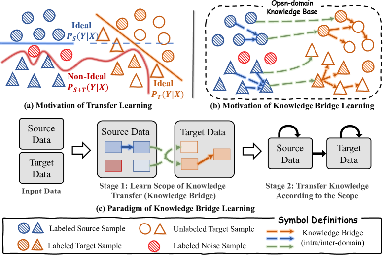
Figure 1. Comparison of Knowledge Bridge Learning (KBL) and Transfer Learning (TL).

The data-hungry problem, characterized by insufficiency and low-quality of data, is a prevalent challenge in real-world scenarios. This challenge presents obstacles for deep learning, because they heavily rely on substantial volumes of high-quality data for effective parameter optimization. Due to the high cost of manual annotation, a feasible way is to find existing high-quality external datasets from other domains to supplement the shortage of target datasets(Saito et al., 2019; Kim and Kim, 2020; Ganin and Lempitsky, 2015; Sun et al., 2011; Bi et al., 2022b; Li et al., 2023). However, external datasets often exhibit significant domain differences compared to the target dataset (e.g., distribution shifts in labels or features). How to improve the performance of deep learning in data-hungry scenarios with the help of external data is a critical research problem.

Transfer learning (TL) (Long et al., 2015; Wilson and Cook, 2020; Gui et al., 2022; Wang et al., 2022; Wu et al., 2022a, 2023b) attempts to transfer knowledge from the source domain data to the target domain data and has gained significant success in various scenarios, e.g., image recognition and text mining (Jin et al., 2020; Saito et al., 2019; Yoon et al., 2022; Zhang et al., 2019; Chen et al., 2009). Specifically, TL methods transfer information at the domain level, i.e., they jointly train models on data from both the source and target domain and diminish the domain difference concurrently. However, these methods have two shortcomings shown in Fig. 1 (a): (1) they are usually built on strong assumptions (Long et al., 2015; Saito et al., 2019), e.g., assuming that data from different domains have the same conditional distribution (detailed analysis in Sec. 3.1). These assumptions, however, are usually unsatisfied in real scenarios, thus leading to limited choices for available source domain data or even no satisfied source domain data (Wilson and Cook, 2020); (2) domain-level information contains both useful and noisy information, and transferring source information indiscriminately may restrict the modeling capacity. Due to the above two limitations, the paradigm of domain-level knowledge transfer may lead to poor generalization ability on the target domain.

Inspired by the idea of Graph Neural Networks (GNNs) that learn node representations by transferring information from neighbors (Cai et al., 2021; Sun et al., 2014; Duval and Malliaros, 2022; Ren et al., 2022; Liang et al., 2022b, a), we redefine the paradigm of knowledge transfer and propose the framework of Knowledge Bridge Learning (KBL). In Fig. 1 (b), we regard both the source domain and target domain as an open-domain knowledge base that consists of diverse samples. Each sample serves as a query, which is similar to information retrieval models that retrieve relevant items for a query from a collection of open-domain documents. We extract valuable knowledge (samples in the open domain) for each query (a target sample) and bridge them. Such bridges form the scope of knowledge transfer, namely Bridged-Graph, specifically identifying which samples in the open-domain data contain knowledge that is beneficial for the samples in the target domain. Then we transfer knowledge under the guidance of the learned scope (Bridged-Graph) with GNNs. Overall, KBL consists of two steps as illustrated in Fig. 1 (c): learning the scope of knowledge transfer (i.e., Bridged-Graph) first and then transferring useful knowledge according to the learned scope.

The paradigm of KBL has the following unique advantages: (1) KBL breaks the limitations of transfer learning that assume a domain-invariant posterior distribution between the source and target domains. KBL aims at learning a knowledge-enhanced posterior distribution for target domain, i.e., learning $P_{T}\left(Y|X,\mathcal{K}(X)\right)$ where $\mathcal{K}(X)$ is the knowledge of each sample, rather than jointly learning a shared posterior distribution $P_{S+T}(Y|X)$ of source and target domains. (2) KBL can filter the noise of source domains by fine-grained knowledge transfer scoped by Bridged-Graph.

Under the paradigm of Knowledge Bridge Learning, we propose a novel Bridged-Graph Neural Network (Bridged-GNN) model. Bridged-GNN consists of two main components: the Adaptive Knowledge Retrieval (AKR) module and the Graph Knowledge Transfer (GKT) module. The Adaptive Knowledge Retrieval (AKR) module aims to retrieve beneficial samples that contain useful knowledge for the given sample from both the source and target domains. Then we view these retrieved beneficial samples, which may be from the source domain (inter-domain) or target domain (intra-domain), as knowledge for each target benefited sample and connect such directed ”beneficial-benefited” edges to construct the Bridged-Graph. Bridged-Graph is a structure of data that defines the scope of knowledge transfer. Besides, we propose a scalable training algorithm to optimize the parameters of AKR. In the next step, we use a Graph Knowledge Transfer (GKT) module to transfer sample-wise knowledge on the Bridged-Graph. Here we can use any message-passing-based GNNs as the GKT module.

According to whether there exist intra-domain and inter-domain relations between samples of original data, we divide knowledge transfer into three scenarios (see Fig. 2): (a) un-relational data, namely $UD$, (b) relational data with intra-domain relations and without inter-domain relations, namely $RD_{intra}$, (c) relational data with both intra-domain relations and inter-domain relations, namely $RD_{intra\&inter}$. We conduct comprehensive experiments of three scenarios on four real-world datasets (Company, Twitter, Facebook100, Office31) and a synthetic dataset. The results consistently show that Bridged-GNN gains significant improvements in all three scenarios.

The main contributions of this paper are summarized as follows:

• We redefine the paradigm of knowledge transfer as Knowledge Bridge Learning (KBL) that conducts sample-wise knowledge transfers within the learned scope.

• We propose a novel Bridged-GNN model under the paradigm of KBL to transfer knowledge effectively in three different scenarios.

• Comprehensive experiments on real-world and synthetic datasets demonstrate the effectiveness of our method.

Figure 2. Knowledge Bridge Learning in three scenarios.

(a) Twitter

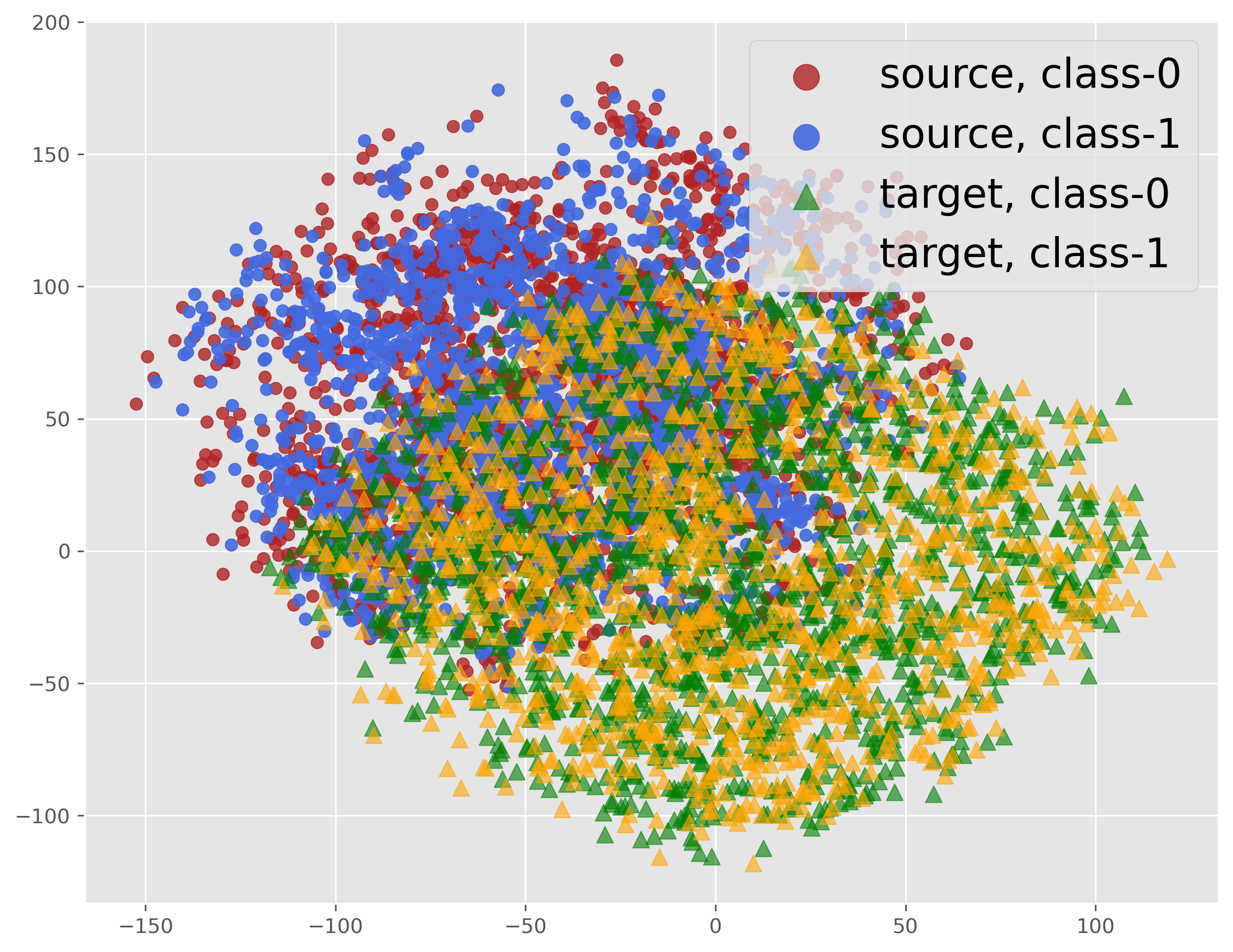
(b) Company

(c) FB (Hamilton$\rightarrow$Caltech)

(d) FB (Howard$\rightarrow$Simmons)

(e) Sync Dataset

Figure 3. T-SNE visualization of the domain shift in real-world datasets and synthetic dataset. To better show the difference in feature distribution conditioned on different classes, we only use samples from the first two classes to draw scatter plots.

2. Preliminary

In this section, we introduce GNNs and our problem definitions.

2.1. Graph Neural Networks

Graph, denoted as $G(V,E,X,Y)$, is composed of nodes $V$ and edges $E$, where $V=\{v_{i}|v_{i}\in V\}$ and $E=\{e_{ij}=(v_{i},v_{j})|v_{i}\ \text{and}\ \ v_{j}$ $\text{is connected}\}$. $N=|V|$ is the number of nodes, $X\in\mathbb{R}^{N\times D_{in}}$ is the feature matrix and $Y\in\mathbb{R}^{N\times 1}$ is the labels of all nodes.

Graph Neural Networks (GNNs) aim at learning representations for nodes on the graph. Given a graph $\mathbf{G}(V,E,X,Y)$ as input, GNNs learn node representations by iteratively aggregating information from neighbors. Current mainstream GNNs update node representations with the following function:

(1) $$H^{(l)}_{i}={\color[rgb]{0,0,0}\texttt{Combine}}\left(H^{(l-1)}_{i},{\color[rgb]{0,0,0}\texttt{AGG}}\big{(}\{H^{(l-1)}_{i},H_{j}^{(l-1)}|v_{j}\in\mathcal{N}(v_{i})\}\big{)}\right)$$

Where $H^{(l)}_{i}$ is the node representation vector at $l$-th layer, AGG denotes the neighborhood aggregation function, and Combine denotes the combination function that updates node representation with the aggregated neighborhood feature and the central node feature.

2.2. Problem Definitions

We introduce the scenarios of Knowledge Transfer and the definitions of Knowledge Bridge Learning in this section.

2.2.1. Scenarios of Knowledge Transfer

Knowledge transfer can be leveraged in three scenarios as shown in Fig. 2: (a) un-relational data ($UD$) represents the scenario where both source domain and target domain are non-graph data, denoted by $(X^{S},Y^{S})$ and $(X^{T},Y^{T})$. (b) data with intra-domain relations and without inter-domain relations ($RD_{intra}$) represents the scenario of both source domain and target data are graph data and there are no edges between the two graphs, denoted by $G^{S}(X^{S},Y^{S},E^{S})$ and $G^{T}(X^{T},Y^{T},E^{T})$. (c) data with intra-domain relations and inter-domain relations ($RD_{intra\&inter}$) represents the scenario that both intra-domain and inter-domain edges exist in the original graph, denoted by $G(\{X^{S},X^{T}\},\{Y^{S},Y^{T}\},E)$. Existing transfer learning methods usually focus on un-relational scenarios, e.g., images.

2.2.2. Knowledge Bridge Learning (KBL)

As shown in Fig. 1 (c), KBL is a new paradigm of knowledge transfer, which regards both the source domain and target domain as an open-domain knowledge base, and takes each sample as a query. KBL first learns a scope of knowledge transfer by querying the open-domain knowledge base and then transfers knowledge within the learned scope. In this paper, we propose to use Bridged-Graph to represent the scope of knowledge transfer:

Definition 2.1 (Bridged-Graph).

Bridged-Graph is represented as $G_{\text{bridged}}=(V^{S},V^{T},X^{S},X^{T},Y^{S},Y^{T},E)$ which defines the scope of knowledge transfer with beneficial-benefited relations between samples, where $V^{S}$ ($V^{T}$) is the sample/node set of the source (target) domain, $X^{S}\in\mathbb{R}^{N^{S}\times D^{in}}$ ($X^{T}\in\mathbb{R}^{N^{D}\times D^{in}}$) is the feature matrix of the source (target) domain, $Y^{S}$ ($Y^{T}$) is the labels of the source (target) domain, $E=\{e_{ij}=(v_{i},v_{j})|v_{i},v_{j}\in V^{S}\cup V^{T}\}$ is the beneficial-benefited edge set, where the edge $e_{ij}$ indicates $v_{i}$ contains useful knowledge for $v_{j}$ (i.e., $v_{i}$ is a beneficial node for $v_{j}$).

Note that edges on the Bridged-Graph include both intra-domain edges and inter-domain edges, namely ”Knowledge Bridge”. Then we define Knowledge Bridge Learning (KBL) as follows:

Definition 2.2 (Knowledge Bridge Learning).

Knowledge Bridge Learning (KBL) is a paradigm of knowledge transfer. KBL first learns a Bridged-Graph from data to define the valid scope of knowledge transfer and then transfers knowledge on the Bridged-Graph from beneficial nodes to benefited nodes.

In all three scenarios shown in Fig. 2, KBL learns a Bridged-Graph to scope the knowledge transfer, while the difference of the learned Bridged-Graph in the three scenarios is that we will reuse the original edges in relational data which are suitable for knowledge transfer. For un-relational data scenarios, we learn Bridged-Graph from scratch with the original isolated samples. For $RD_{intra}$ scenario, we learn Bridged-Graph by adding new knowledge bridges and reusing original intra-domain edges. For $RD_{intra\&inter}$ scenario, we further reuse the original inter-domain edges.

3. Methodology

In this section, we introduce the motivation and architecture of our Bridged Graph Neural Network (Bridged-GNN) under the guidance of Knowledge Bridge Learning.

3.1. Motivations of Knowledge Bridge Learning

3.1.1. Irregular Domain Shift in Real-world Data

Domain shift problem usually refers to the difference in the joint distribution (i.e., $P(X,Y)$) between the source domain and the target domain. However, directly modeling the joint distribution is difficult with few target labels, and some methods (Long et al., 2013, 2017) use pseudo labels to estimate the pseudo joint distribution, which is sensitive to noises and results in estimation bias. As one of the most representative transfer learning methods, Domain Adaptation (DA) simplifies the problem by making assumptions based on the Bayes formula:

$$P(X,Y)=P(X|Y)P(Y)=P(Y|X)P(X).$$

DA methods usually assume that the source domain and target domain share invariant conditional distribution ($P(X|Y)$ or $P(Y|X)$), while having different marginal distribution ($P(X)$ or $P(Y)$)(Wilson and Cook, 2020; Saito et al., 2019; Long et al., 2015). And the mainstream framework of DA, including the unsupervised and the semi-supervised settings, is to jointly train a shared model on the source and target domains while aligning the marginal distribution discrepancy, assuming a shared posterior distribution of source and target domains during this process.

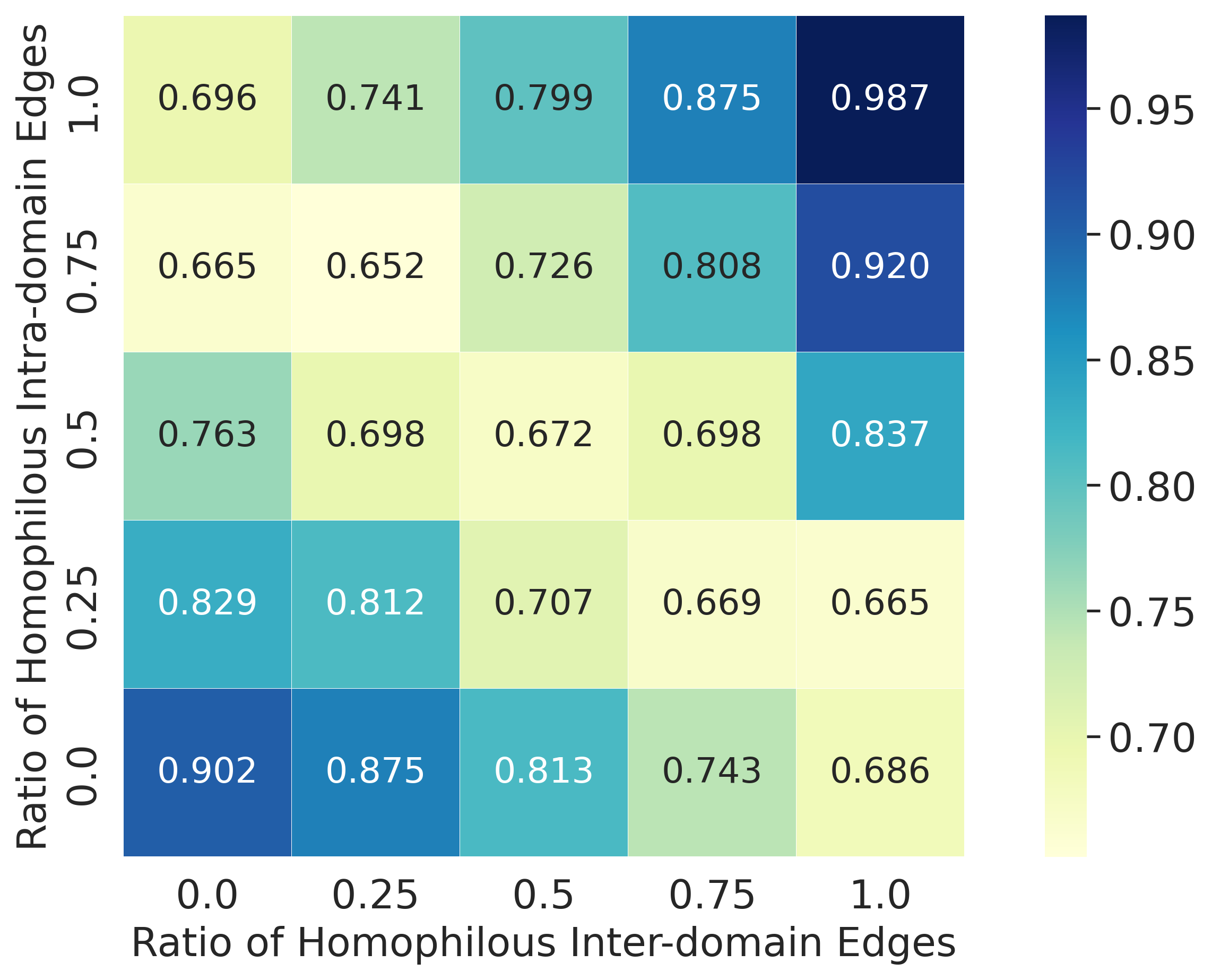
(a) Twitter

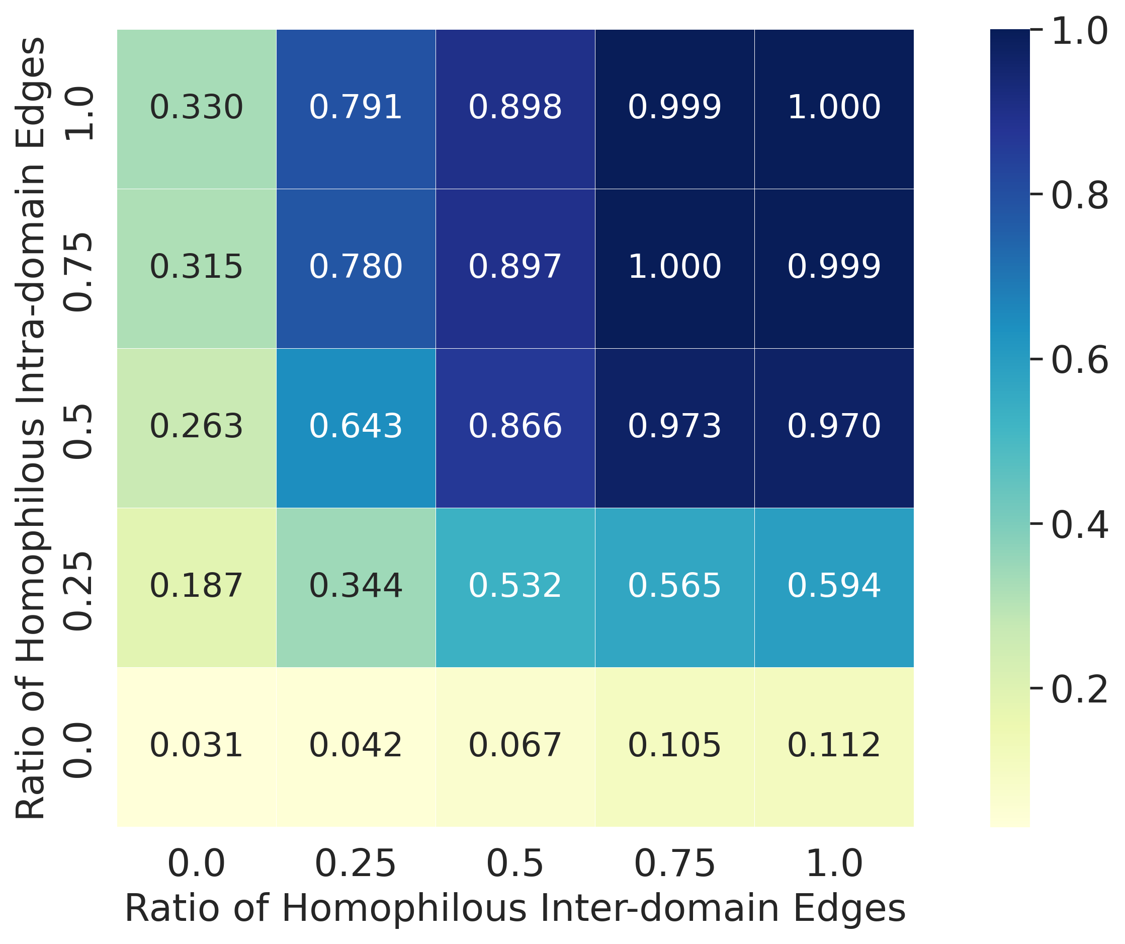
(b) Office31 (A$\rightarrow$D)

Figure 4. Results on Bridged-Graphs constructed via randomly adding edges and controlling the ratio of homophilous neighbors, including homophilous ratio of intra-domain edges (Y-axis) and inter-domain edges (X-axis).

However, we observed that this assumption is hard to be satisfied in real-world data, and the conditional distribution between the source domain and target domain may have significant differences. As shown in Fig. 3, we visualize the features of five datasets used in this paper with the T-SNE algorithm. In each scatter plot, we distinguish the samples of different classes and different domains with four different colors. For the Facebook100 dataset which has multiple classes, we only select the samples of the first two classes to present the results more clearly. Fig. 3 (a)$\sim$(d) are from four real-world datasets, we find there exist significant domain differences on both the conditional distribution and marginal distribution in these datasets. These evidences indicate that we cannot ignore the conditional distribution differences in the real data, and motivate us to design a new paradigm.

As shown in Fig. 1 (c), learning a shared posterior distribution ($P_{S+T}(Y|X)$) on source and target domains is sensitive to the conditional distribution shift and noise data. Different from previous transfer learning, our Knowledge Bridge Learning aims at enriching the sample information by injecting knowledge from other samples, and changing the paradigm of learning shared posterior distribution into learning a knowledge-enhanced posterior distribution for target domain,i.e., $P_{T}\left(Y|X,\mathcal{K}(X)\right)$, where $\mathcal{K}(X)$ is the external knowledge of samples (source nodes on the Bridged-Graph).

3.1.2. Effectiveness of Knowledge Transfer on Bridged-Graph

Knowledge Bridge Learning aims to learn a scope named Bridged-Graph and transfer knowledge via this graph. Such a graph determines the upper bound of performance improvement gained by knowledge transfer. Therefore, we first validate the effectiveness of our KBL by a synthetic Bridged-Graph. Specifically, we generated many Bridged-Graphs on two real-world datasets (Twitter (Xiao et al., 2020) and Office31 (Saito et al., 2019)) by randomly adding edges between samples while controlling the ratio of homophilous neighbors (neighbors of the same class). For each synthetic Bridged-Graph, we randomly add 8 neighbors $v_{i}$ as source nodes (4 nodes in $V^{S}$ and 4 nodes in $V^{T})$ for each target domain sample $v_{j}\in V^{T}$, and only add 4 neighbors from $V^{S}$ as source nodes for each source domain sample $v_{j}\in V^{S}$. Then we use GraphSAGE (Hamilton et al., 2017) as the Graph Knowledge Transfer module of KBL to transfer knowledge from source nodes to target nodes and record the test accuracy of node classification. As shown in Fig. 4, when the homophilous ratio of intra-domain edges and inter-domain edges tends to 1.0 at the same time, the test accuracy nearly reaches 100%, which demonstrates the effectiveness of our motivations (knowledge transfer on Bridged-Graph).

Figure 5. Overview of Bridged-GNN

3.2. Overview of Bridged-GNN

Guided the paradigm of Knowledge Bridge Learning in Sec.2.2.2, we propose Bridged-GNN and show its overview in Fig. 5. Bridged-GNN is implemented in a two-stage manner which is composed of two main components: Adaptive Knowledge Retrieval (AKR) module and Graph Knowledge Transfer (GKT) module. Specifically, Bridged-GNN first learns a Bridged-Graph to determine the scope of knowledge transfer, and then uses a GNN model as plug-in to transfer knowledge on the Bridged-Graph. Bridged-GNN model can be applied to all three scenarios in Fig. 2.

3.3. Adaptive Knowledge Retrieval (AKR)

In the first step, we need to learn the Bridged-Graph to determine the scope of knowledge transfer. We mainly focus on the classification tasks in this paper, and the required useful knowledge of a specified sample is mainly contained in the homophilous samples of the same class (validated in Sec. 3.1.1)(Bi et al., 2022a; Guo et al., 2023a; Yang et al., 2023; Bashardoust et al., 2023; Begga et al., 2023; Pan and Kang, 2023). Considering the candidates of beneficial samples are from different domains, we design an Adaptive Knowledge Retrieval (AKR) module. Given arbitrarily specified sample as a query, AKR retrieves top-K beneficial samples from all candidates as intra-domain/inter-domain knowledge for the query sample.

3.3.1. Architecture of AKR

The AKR module first learns the similarities of samples for knowledge retrieval, which may be from the same domain (intra-domain) or different domains (inter-domain), and then retrieve beneficial samples for each sample (query) with the learned similarities to construct the Bridged-Graph. As shown in Fig. 6, we design a twin-flow architecture for the AKR module. AKR is composed of the source encoder, the target encoder, and a discriminator with the adversarial training strategy.

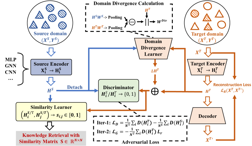
Figure 6. Architecture of the Adaptive Knowledge Retrieval (AKR) module. The blue (orange) arrows denote the data flow of the source (target) domain.

First, a source encoder $\mathcal{F}^{src}(\cdot)$ and a target encoder $\mathcal{F}^{tar}(\cdot)$ are designed to encode the input data from the source domain and target domain respectively:

(2) $$\left\{\begin{aligned} H^{S}&=\mathcal{F}^{src}(X^{S},\cdots)\\ H^{T}&=\mathcal{F}^{tar}(X^{T},\cdots)\\ \end{aligned}\right.$$

where $X^{S}\in\mathbb{R}^{N^{src}\times D^{in}}$ and $X^{T}\in\mathbb{R}^{N^{tar}\times D^{in}}$ represent the sample features of the source domain and target domain, $H^{S}$ and $H^{T}$ denote the hidden representations of the source domain and target domain. Besides, for graph data, the input data also includes the adjacent matrix $A^{S}\in\mathbb{R}^{N^{S}\times N^{S}}$ and $A^{T}\in\mathbb{R}^{N^{T}\times N^{T}}$. According to the different types of input data (e.g., text, graph, image), we can choose appropriate backbone networks (e.g., DNN, GNN, CNN) as encoders to fit the data better.

Then we transform the representations of target domain samples ($H^{T}$) into the same feature space as the source domain. We achieve this by using a Domain Divergence Learner module to learn the domain difference variable (i.e., the domain difference between the source domain and target domain) which considers the personalized information of each target domain sample and the overall difference between the source domain and target domain representations:

(3) $$\Delta H^{T}=\left[{\color[rgb]{0,0,0}\texttt{Pooling}}(H^{S}W^{S})-{\color[rgb]{0,0,0}\texttt{Pooling}}(H^{T}W^{T})\ ||\ H^{T}\right]\cdot W^{Div},$$

where Pooling is the SUM pooling function. Then we can get the transformed target domain representations denoted as $\widetilde{H}^{T}$:

(4) $$\widetilde{H}^{T}=H^{T}+\Delta H^{T}$$

In order to prevent the target domain representations encoded by the target domain encoder from forgetting the original target domain information, we add a target domain decoder to form an Auto-Encoder and further optimize it by reconstruction loss:

(5) $$\mathcal{L}_{R}=\frac{1}{N^{T}}\cdot\sum_{i=1}^{N^{T}}\left({\color[rgb]{0,0,0}\texttt{Decoder}}(X^{T}_{i})-X^{T}_{i}\right)^{2}$$

Then we use an adversarial loss to make sample pairs from intra-domain and inter-domain measured in a common semantic space. Specifically, we use a discriminator (D) to distinguish the samples from the source domain and target domain, and calculate adversarial loss iteratively:

(6) $$\left\{\begin{aligned} \mathcal{L}_{D}&=\frac{1}{N^{T}}\sum_{i=1}^{N^{T}}{\color[rgb]{0,0,0}\texttt{D}}(\widetilde{H_{i}}^{T})-\frac{1}{N^{S}}\sum_{i=1}^{N^{S}}{\color[rgb]{0,0,0}\texttt{D}}\left({\color[rgb]{0,0,0}\texttt{detach}}(H_{i}^{S})\right)\\ \mathcal{L}_{G}&=-\frac{1}{N^{T}}\sum_{i=1}^{N^{T}}{\color[rgb]{0,0,0}\texttt{D}}(\widetilde{H_{i}}^{T})\end{aligned}\right.$$

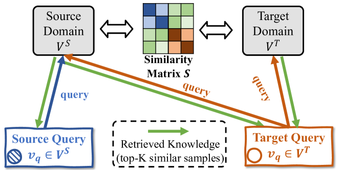
Figure 7. Knowledge retrieval (top-K beneficial samples).

With the obtained source domain representations $H^{S}$ and the transformed target domain representations $\widetilde{H}^{T}$, which belong to the same feature space, we then train a cosine similarity learner module to learn the pair-wise similarity of arbitrary sample pair:

(7) $$S_{i,j}=\Gamma_{\text{Cosine}}(W^{\text{Sim}}\widehat{H}^{S+T}_{i},W^{\text{Sim}}\widehat{H}^{S+T}_{j}),\quad\widehat{H}^{S+T}=\begin{bmatrix}H^{S}\\ \widetilde{H}^{T}\end{bmatrix}$$

Where $S_{i,j}$ represents the similarity between nodes $v_{i}$ and $v_{j}$ ($v_{i}$ and $v_{j}$ may be from the same domain or different domains). $\Gamma_{\text{Cosine}}(\cdot,\cdot)$ represents the cosine similarity function. Finally, we get a similarity matrix $S\in\mathbb{R}^{N\times N}$ where $N=N^{S}+N^{T}$. Then given any query sample $v_{q}\in\{V^{S}\cup V^{T}\}$, we can retrieve top-K (K is a hyperparameter) similar samples from $V^{S}\cup V^{T}$ as the knowledge of $v_{q}$:

(8) $$\mathcal{K}(v_{q})=\{<v_{i},v_{q}>|v_{i}\in\{V^{S}\cup V^{T}\},S_{i,q}\in{\color[rgb]{0,0,0}\texttt{top-K}}(S_{:,q})\}$$

As shown in Fig. 7, considering the insufficiency and low quality of target domain data, we retrieve knowledge for each source domain sample from source domain only, while retrieving knowledge for each target domain sample from both source and target domains. We optimize the AKR module by binary cross entropy (BCE) loss:

(9) $$\mathcal{L}_{CLF}=\frac{1}{N^{\text{pair}}}\sum_{v_{i},v_{j}\in\{V^{S}\cup V^{T}\}}{\color[rgb]{0,0,0}\texttt{BCE}}\left(Y^{\text{pair}}_{ij},\sigma(S_{ij})\right)$$

Where $N^{\text{pair}}$ represents the number of sample pairs $<v_{i},v_{j}>$ used for training, $Y^{\text{pair}}_{ij}=1$ indicates that the pair of samples $<v_{i},v_{j}>$ belong to the same category, otherwise $Y^{\text{pair}}_{ij}=0$. $\sigma(\cdot)$ represents the Sigmoid function. Overall, we leverage $\mathcal{L}_{D}$ to optimize discriminator while fixing the parameters of AKR except for the discriminator, then $\mathcal{L}_{CLF}$ is leveraged together with $\mathcal{L}_{R}$ and $\mathcal{L}_{G}$ (i.e., $\mathcal{L}_{R}+\mathcal{L}_{G}+\mathcal{L}_{CLF}$) to optimize the AKR except for the discriminator. These two steps are performed iteratively. In principle, our method can be applied to any machine learning tasks (e.g., classification and regression tasks).

3.3.2. Scalable optimization strategy with balanced sampling

Considering that the number of possible sample pairs is the square of the universal sample size ($N^{2}$), which is infeasible to train with full-batch with a large $N$. Besides, sample pairs of datasets with multiple classes are extremely unbalanced, i.e., negative pairs with different labels are far more than positive pairs with the same label.

To tackle the scalability and imbalance problems, we design a scalable optimization strategy with Balanced Pair-wise Sampling (BPS). Specifically, we use the BPS algorithm shown in Algo. 1 to sample $N^{\text{pair}}$ intra-domain sample pairs in the source domain and target domain respectively (setting $X^{1}=X^{2}=X^{S},Y^{1}=Y^{2}=Y^{S}$ and $X^{1}=X^{2}=X^{T},Y^{1}=Y^{2}=Y^{T}$). And we sample $N^{\text{pair}}$ inter-domain (source$\rightarrow$target) sample pairs (setting $X^{1}=X^{S},X^{2}=X^{T},Y^{1}=Y^{S},Y^{2}=Y^{T}$). Then we get a total of $3N^{\text{pair}}$ pairs of samples in each iteration. We set Max_Class_Num to 10 for all datasets. The BPS algorithm can guarantee the same number of positive pairs and negative pairs in each mini-batch. Besides, we can set an arbitrary $N^{\text{pair}}$ according to the data size.

Input: $\text{Data}_{1}$: ($X^{1}$, $Y^{1}$), $\text{Data}_{2}$: ($X^{2}$, $Y^{2}$), Sample_Size: $N^{\text{pair}}$, Max_Class_Num: $M$.

Output: $N^{\text{pair}}$ pairs of sample: $\left\{<x_{i}\in X^{1},x_{j}\in X^{2}>,Y^{\text{pair}}_{ij}=\mathbf{1}_{Y^{1}_{i}==Y^{2}_{j}}\right\}$

1 Random select $M$ categories $\mathcal{C}_{y}=\{y_{1},y_{2},\cdots y_{M}\}$ in all possible class of $Y^{1}\cup Y^{2}$.

2 Output $\leftarrow\{\}$.

3 foreach $Y_{\text{from}}\in\mathcal{C}_{y}$ do

4       foreach $Y_{\text{to}}\in\mathcal{C}_{y}$ do

5             if $Y_{\text{from}}==Y_{\text{to}}$ then

6                   $N_{\text{batch}}\leftarrow\lfloor\frac{0.5*N^{\text{pair}}}{M}\rfloor$

7            else

8                   $N_{\text{batch}}\leftarrow\lfloor\frac{0.5*N^{\text{pair}}}{M*(M-1)}\rfloor$

9            1. Randomly sampling $N_{\text{batch}}$ samples from $\{X^{1}_{i}|Y^{1}_{i}==Y_{\text{from}}\}$, denoted as ${\color[rgb]{0,0,0}\texttt{Batch}}_{1}$.

10             2. Randomly sampling $N_{\text{batch}}$ samples from $\{X^{2}_{i}|Y^{2}_{i}==Y_{\text{to}}\}$, denoted as ${\color[rgb]{0,0,0}\texttt{Batch}}_{2}$.

11             3. $X^{\text{pair}}$ $\leftarrow\{<x_{i},x_{j}>|x_{i}\in{\color[rgb]{0,0,0}\texttt{Batch}}_{1},x_{j}\in{\color[rgb]{0,0,0}\texttt{Batch}}_{2}\}$

12             Output $\leftarrow\{{\color[rgb]{0,0,0}\texttt{Output}}\cup X^{\text{pair}}\}$.

13      

Algorithm 1 Balanced Pair-wise Sampling (BPS)

3.4. Graph Knowledge Transfer (GKT)

Leveraging the retrieved knowledge in the previous step, we can construct the Bridged-Graph defined in Sec. 2.2.2. Then we use a GNN model to transfer knowledge on the Bridged-Graph.

3.4.1. Conversion from Retrieved Knowledge to Bridged-Graph

We further convert the retrieved knowledge (see Eq. 8 and Fig. 7) into a Bridged-Graph. For all three scenarios of Knowledge Transfer shown in Fig. 2, we view each sample as a node and add edges from top-K retrieved beneficial nodes to each target node, i.e. a KNN-Graph, where K is a hyperparameter set by grid search in {4, 8, 16, 20} in our experiments. Besides, we also reuse the original edges that are suitable for knowledge transfer in two relational data scenarios ($RD_{intra}$, $RD_{intra\&inter}$). Specifically, we remove original edges with similarities lower than the threshold $\epsilon$ (we set $\epsilon$ as the 25% quantile number of the similarity matrix in our experiments and can adjust it according to the actual situations), and then reuse the remaining edges in the Bridged-Graph.

3.4.2. GNN for Knowledge Transfer on Bridged-Graph.

With the learned Bridged-Graph that defines the scope of knowledge transfer, we then use a Graph Neural Network model to transfer knowledge from beneficial samples to benefited samples. At this step, all message-passing-based GNNs can be used as a plug-in for the GKT module. We use GNNs as our GKT module because the neighborhood aggregation framework (see Eq. 1) of GNNs just matches our motivation (see Sec. 3.1.1) to learn a knowledge-enhanced posterior distribution for the target domain:

(10) $$P_{T}\left(y_{i}|x_{i},\mathcal{K}(x_{i})\right)\rightarrow P_{T}\left(y_{i}|{\color[rgb]{0,0,0}\texttt{Combine}}\left(x_{i},{\color[rgb]{0,0,0}\texttt{AGG}}\left(\{x_{j}|v_{j}\in\mathcal{N}(v_{i})\}\right)\right)\right)$$

The AGG function of GNN is used to aggregate the retrieved knowledge from AKR, while the Combine function of GNN is used to combine the original sample feature and the aggregated knowledge. Considering that there exist multi-domain nodes on the Bridged-Graph, we mainly use KTGNN (Bi et al., 2023b) which considers node-level domain shift as the GKT module in Bridged-GNN. And we also evaluate the performance of other mainstream GNNs (e.g., GCN, GAT, GCNII) (see Table 3 and Table 4).

4. Experiments

In this section, we compare Bridged-GNN with other state-of-the-art methods on the three knowledge transfer scenarios in Fig. 2.

4.1. Datasets

We conduct experiments on five datasets, including four real-world datasets and a synthetic dataset. The basic information is shown in Table 1, and a brief introduction of datasets is as follows: :

Table 1. Basic information of the datasets used in this paper. $N^{S}$ and $N^{T}$ denote the number of samples in the source domain and target domain. $D^{in}$ is the feature dimension.

Dataset	$N^{S}$	$N^{T}$	$D^{in}$	Edge Num	Class Num
$\text{Twitter}_{UD}$	581	20230	300	0	2
Office31 (A$\rightarrow$W)	2817	888	image	0	31
Office31 (A$\rightarrow$D)	2817	591	image	0	31
Sync-$UD$	600	300	64	0	2
FB (Hamilton$\rightarrow$Caltech)	2314	769	6	258735	7
FB (Howard$\rightarrow$Simmons)	4047	1518	6	538924	7
Sync-$RD_{intra}$	600	300	64	2414	2
$\text{Twitter}_{\text{Graph}}$	581	20230	300	915438	2
Company	3987	6654	33	116785	2
Sync-$RD_{intra\&inter}$	600	300	64	3414	2

Table 2. Experiments of classification on target domain samples in the scenario of un-relational data ($UD$ in Fig. 2 (a)). The meaning of the model with subscripts can be found at Sec. 4.2.

Dataset	$\text{Twitter}_{UD}$		Office31 (A$\rightarrow$D)		Office31 (A$\rightarrow$W)		Sync-$UD$
Method $\backslash$ Metric	F1-macro	AUC	F1-macro	F1-micro	F1-macro	F1-micro	F1-macro	AUC
$\text{DNN}_{\text{T}}$	70.02$\pm$1.16	76.68$\pm$1.11	91.02$\pm$1.20	91.53$\pm$1.39	88.15$\pm$0.55	88.68$\pm$0.93	81.08$\pm 0.92$	90.58$\pm 0.29$
$\text{DNN}_{\text{S}\rightarrow\text{T}}$	70.62$\pm$1.03	76.08$\pm$0.89	91.32$\pm$0.83	91.58$\pm$0.63	88.19$\pm$0.63	88.79$\pm$0.68	81.56$\pm 1.02$	90.93$\pm 0.78$
$\text{DNN}_{\text{S+T}}$	70.85$\pm$1.31	76.12$\pm$1.38	90.53$\pm$0.62	89.93$\pm$0.62	87.83$\pm$0.32	88.53$\pm$0.59	78.99$\pm 0.26$	90.06$\pm 1.83$
DANN	74.29$\pm$0.77	78.21$\pm$1.21	91.68$\pm$0.75	92.02$\pm$0.88	88.58$\pm$0.28	88.92$\pm$0.53	81.87$\pm 0.98$	91.23$\pm 0.77$
DAN	74.89$\pm$0.87	78.08$\pm$0.56	91.38$\pm$0.52	91.87$\pm$0.66	88.69$\pm$0.75	88.91$\pm$0.98	82.03$\pm 1.06$	91.61$\pm 0.73$
CDAN	72.85$\pm$0.96	76.18$\pm$1.03	91.05$\pm$0.39	91.33$\pm$0.42	88.03$\pm$0.56	88.79$\pm$0.93	81.38$\pm 1.32$	90.63$\pm 0.91$
MME	77.63$\pm$0.67	79.82$\pm$1.23	92.08$\pm$0.89	92.13$\pm$0.67	89.08$\pm$0.57	89.17$\pm$0.73	82.33$\pm 1.32$	92.16$\pm 0.92$
APE	76.21$\pm$0.85	78.03$\pm$1.38	91.67$\pm$0.89	91.88$\pm$0.68	89.23$\pm$0.57	89.29$\pm$0.73	82.50$\pm 1.09$	92.21$\pm 1.22$
$\text{S}^{3}\text{D}$	78.39$\pm$1.56	80.87$\pm$1.56	91.87$\pm$1.09	92.23$\pm$0.99	88.98$\pm$0.91	89.02$\pm$0.92	83.08$\pm 1.58$	92.63$\pm 1.77$
$\text{{Bridged-GNN}}_{\backslash\text{{KTGNN}}}$	$\mathbf{82.85}$$\mathbf{\pm 0.76}$	$\mathbf{85.13}$$\mathbf{\pm 0.87}$	93.17$\pm$0.39	93.33$\pm$0.52	89.67$\pm$0.03	90.31$\pm$0.65	$\mathbf{85.47}$$\mathbf{\pm 0.92}$	$\mathbf{95.16}$$\mathbf{\pm 1.24}$

Twitter (Bi et al., 2023b; Xiao et al., 2020): Twitter is a social network dataset that describes the social relations among politicians (source domain) and civilians (target domain) on the Twitter platform. And the goal is to predict the political tendency of civilians. By removing original edges, we also construct the $\text{Twitter}_{UD}$ dataset in un-relational data scenarios.

Office31 (Saito et al., 2019): The Office31 dataset is a mainstream image benchmark for transfer learning. There are three different domains (Amazon, Webcam, and DSLR) in this dataset. We select Webcam and DSLR, which are data-hungry, as the target domain, and use Amazon, which is rich in data, as the source domain, including Office31 (A$\rightarrow$W) and Office31 (A$\rightarrow$D).

FB (Traud et al., 2012): FB (Facebook100) datasets are social networks of 100 different universities in the United States. And the goal is to predict Node identity flags. We view the social network of each university as an independent domain and select two of them to form a cross-network(domain) dataset in $RD_{intra}$ scenarios, including FB (Hamilton$\rightarrow$Caltech) and FB (Howard$\rightarrow$Simmons).

Company (Bi et al., 2023b): Company dataset is a company investment network with 10641 real-world companies in China. We regard listed companies as source domain and unlisted companies as target domain and the goal is to predict the risk status of non-listed companies. And we use this dataset in the $RD_{intra\&inter}$ scenario.

Sync-$UD$/Sync-$RD_{intra}$/Sync-$RD_{intra\&inter}$: We construct 3 synthetic datasets for three scenarios of GKT by randomly sampling points of source and target domains from two distinct Multivariate Gaussian distributions, which are visualized in Fig. 3 (e). The samples of source and target domains in this dataset are designed to have distinct conditional distribution and marginal distribution to validate the motivations described in Sec. 3.1.

4.2. Experimental Settings

Data Settings: Under the semi-supervised classification setting, we use all source domain samples and only few target domain samples as training set for all datasets. For Twitter and Company datasets, we use the same data split as Bi et al. (2023b); For other datasets, we randomly select 20% target domain samples in each class for training, and the remaining samples are further divided into the validation set and test set in equal proportions.

Model Settings: For the scenarios of $RD_{intra}$ and $RD_{intra\&inter}$, we use DNN and other GNNs, including GCN (Kipf and Welling, 2016), GAT (Veličković et al., 2017), GCNII (Chen et al., 2020), OODGAT (Song and Wang, 2022), KTGNN (Bi et al., 2023b), as baselines to encode graph data. The hyperparameters settings of these models all refer to the original papers. We remove the original feature completion module of KTGNN because the missing feature problem is not considered in this paper. For un-relational data scenarios, we also use some optimal transfer learning methods (i.e., DANN (Ganin and Lempitsky, 2015), DAN  citeDAN, CDAN (Long et al., 2018), MME (Saito et al., 2019), APE (Kim and Kim, 2020), $\text{S}^{3}\text{D}$ (Yoon et al., 2022)), where the $\text{S}^{3}\text{D}$ model adopts a sample-wise distillation method for semi-supervised domain adaptation and achieves state-of-the-art performance. For transfer learning methods and the encoder of AWR in Bridged-GNN, we use ResNet34 as the backbone network for Office31 dataset and use 3-layer MLP as the backbone network for other datasets with vector features. For all transfer learning methods, we use the recommended hyperparameters in the original papers and train them all in semi-supervised learning settings. Besides, we also compare models with different training strategies:
 (1) T: train on the target domain only.
 (2) S+T: train on the source and target domain concurrently.
 (3) S$\rightarrow$T: pretrain on source domain and finetune on target domain.
We use subscripts to denote a model trained under a specific strategie (e.g., $\text{DNN}_{\text{T}}$, $\text{DNN}_{\text{S+T}}$, $\text{DNN}_{\text{S}}\rightarrow\text{T}$) and Bridged-GNN with a specific GNN as the GKT module, e.g., $\text{{Bridged-GNN}}_{\backslash\text{{KTGNN}}}$.

Evaluation Metric: For binary-classification datasets (Twitter, Company, Synthetic datasets), we use Binary F1-Score and AUC as evaluation metrics. For multi-classification datasets (FB, Office31), we use Macro F1-Score and Micro F1-Score as evaluation metrics. For all datasets, we evaluate the models by their performance of classifying test samples in the target domain.

Table 3. Experiments of node classification on target domain samples in the scenarios of relational data with only intra-domain relations ($RD_{intra}$ in Fig. 2 (b)). The meaning of the model with subscripts can be found at Sec. 4.2.

Dataset	FB (Hamilton$\rightarrow$Caltech)		FB (Howard$\rightarrow$Simmons)		Sync-$RD_{intra}$
Method	F1-Macro	F1-Micro	F1-Macro	F1-Micro	F1-macro	AUC
$\text{GCN}_{\text{T}}$	76.25$\pm$0.35	85.38$\pm$0.17	55.02$\pm 0.49$	89.55$\pm 0.14$	89.63$\pm 0.77$	94.36$\pm 0.14$
$\text{GCN}_{\text{S+T}}$	75.11$\pm$2.57	85.50$\pm$1.02	50.35$\pm 0.57$	89.49$\pm 0.21$	86.66$\pm 0.90$	93.88$\pm 0.30$
$\text{Bridged-GNN}_{\backslash\text{GCN}}$	87.62$\pm$1.78	90.78$\pm$1.14	62.03$\pm\mathbf{2.56}$	90.29$\pm\mathbf{0.52}$	93.88$\pm$ 0.77	96.80$\pm$0.33
$\text{GAT}_{\text{T}}$	75.13$\pm$0.65	84.78$\pm$0.53	55.31$\pm 0.52$	89.78$\pm 0.72$	90.02$\pm 1.09$	94.55$\pm 0.14$
$\text{GAT}_{\text{S+T}}$	74.23$\pm$1.87	84.31$\pm$1.31	51.89$\pm 0.62$	89.98$\pm 0.85$	87.53$\pm 0.70$	93.63$\pm 1.21$
$\text{Bridged-GNN}_{\backslash\text{GAT}}$	86.32$\pm$1.32	90.58$\pm$1.08	60.67$\pm$1.58	90.57$\pm$0.17	94.67$\pm$ 0.58	97.97$\pm$0.76
$\text{GCNII}_{\text{T}}$	77.23$\pm$1.03	86.89$\pm$0.68	58.19$\pm 0.77$	90.08$\pm 0.23$	90.67$\pm 0.85$	94.21$\pm 0.63$
$\text{GCNII}_{\text{S+T}}$	75.83$\pm$1.03	85.38$\pm$1.12	55.89$\pm 0.98$	90.33$\pm 0.87$	87.61$\pm 1.01$	94.32$\pm 1.21$
$\text{Bridged-GNN}_{\backslash\text{GCNII}}$	86.01$\pm$0.93	90.03$\pm$1.33	62.87$\pm$1.55	90.67$\pm$0.53	94.32$\pm$ 0.58	97.78$\pm$0.62
$\text{Bridged-GNN}_{\backslash\text{KTGNN}}$	88.23$\pm$0.88	91.51$\pm$0.79	66.37$\pm$0.23	91.10$\pm$0.73	95.55$\pm$0.49	97.97$\pm$0.33

Table 4. Experiments of node classification on target domain samples in the scenarios of relational data with both intra-domain and inter-domain relations ($RD_{intra\&inter}$ in Fig. 2 (c)). The meaning of the model with subscripts can be found at Sec. 4.2.

Dataset	$\text{Twitter}_{\text{Graph}}$		Company		Sync-$RD_{intra\&inter}$
Method $\backslash$ Metric	F1-macro	AUC	F1-macro	AUC	F1-macro	AUC
$\text{DNN}_{\text{T}}$	70.02$\pm$1.16	76.68$\pm$1.11	57.01$\pm 0.42$	56.35$\pm 0.55$	81.08$\pm 0.92$	90.58$\pm 0.29$
$\text{DNN}_{\text{S}\rightarrow\text{T}}$	70.62$\pm$1.03	76.08$\pm$0.89	57.63$\pm 0.42$	57.01$\pm 0.55$	81.56$\pm 1.02$	90.93$\pm 0.78$
$\text{DNN}_{\text{S+T}}$	70.85$\pm$1.31	80.12$\pm$1.38	57.23$\pm 0.38$	56.71$\pm 0.43$	78.99$\pm 0.26$	91.06$\pm 1.83$
GCN	80.19$\pm$0.87	86.88$\pm$1.23	57.60$\pm 0.49$	57.83$\pm 0.93$	79.67$\pm 2.66$	90.53$\pm 0.59$
GAT	82.31$\pm$1.56	87.88$\pm$1.21	57.98$\pm$0.43	58.40$\pm$0.43	82.78$\pm 1.26$	93.08$\pm 2.03$
GraphSAGE	85.35$\pm$1.32	92.07$\pm$1.08	59.21$\pm 0.93$	61.55$\pm 1.78$	91.69$\pm 1.78$	95.87$\pm 0.63$
GCNII	83.85$\pm$1.17	90.67$\pm$1.32	58.21$\pm 0.88$	60.06$\pm 0.63$	89.98$\pm 0.26$	95.07$\pm 0.31$
OODGAT	85.42$\pm$2.01	92.67$\pm$1.60	60.05$\pm 0.89$	61.37$\pm 0.92$	88.79$\pm 1.77$	93.58$\pm 1.33$
KTGNN	86.60$\pm$1.21	93.38$\pm$1.60	61.78$\pm 0.53$	63.55$\pm 0.65$	93.33$\pm$0.37	96.38$\pm$0.28
$\text{{Bridged-GNN}}_{\backslash\text{{KTGNN}}}$	87.72$\mathbf{\pm 0.80}$	95.32$\mathbf{\pm 1.03}$	63.06$\mathbf{\pm 0.49}$	65.61$\mathbf{\pm 0.58}$	96.67$\mathbf{\pm 0.13}$	99.56$\mathbf{\pm 0.37}$

4.3. Main Experiments

Analysis of experiments on the three main scenarios is as follows.

4.3.1. Results of Knowledge Transfer in $UD$ scenarios

As shown in Table 2, we conduct experiments on four un-relational datasets, including three real-world datasets ($\text{Twitter}_{UD}$, Office31 (A$\rightarrow$D), Office31 (A$\rightarrow$W)) and one synthetic dataset Sync-$UD$. Our $\text{Bridged-GNN}_{\text{KTGNN}}$ gains significant improvements of classification performance on all datasets, e.g., gains $4.46\%$ improvements of F1-macro on $\text{Twitter}_{UD}$ dataset. Compared with other baseline methods and state-of-the-art transfer learning methods, our method gains the best performance in the scenarios of knowledge transfer on un-relational data ($UD$).

4.3.2. Results of Knowledge Transfer in $RD_{intra}$ scenarios

As shown in Table 3, we conduct experiments on three cross-network datasets, including two real-world datasets from Facebook social networks (FB (Hamilton$\rightarrow$Caltech), FB (Howard$\rightarrow$Simmons)) and one synthetic dataset Sync-$RD_{intra}$. Considering most graph neural networks are not designed for cross-network graph representation learning, we compare our Bridged-GNN with two other learning frameworks (T and S+T, see Sec. 4.2) to validate the gain of performance caused by Bridged-GNN, i.e., our idea of ”bridging cross-networks samples”. The results show that all variants of $\text{Bridged-GNN}_{*}$ combined with a specifical GNN model (e.g., GCN, GAT, GCNII, KTGNN) gain significant improvements in classification performance on all datasets. By bridging originally independent graphs, our method gains the best performance in scenarios of intra-domain relational data ($RD_{intra}$).

4.3.3. Results of Knowledge Transfer in $RD_{intra\&inter}$ scenarios

As shown in Table 4, we conduct experiments on two real-world graph datasets ($\text{Twitter}_{\text{Graph}}$, Company) and a synthetic dataset Sync-$RD_{intra\&inter}$. Compared with other mainstream GNNs, our $\text{Bridged-GNN}_{\text{KTGNN}}$ gains significant improvements in classification tasks on all graph datasets. By building a Bridged-Graph based on the original graph structure, our method gains the best performance in the scenarios of relational data with both intra-domain and inter-domain relations ($RD_{intra\&inter})$.

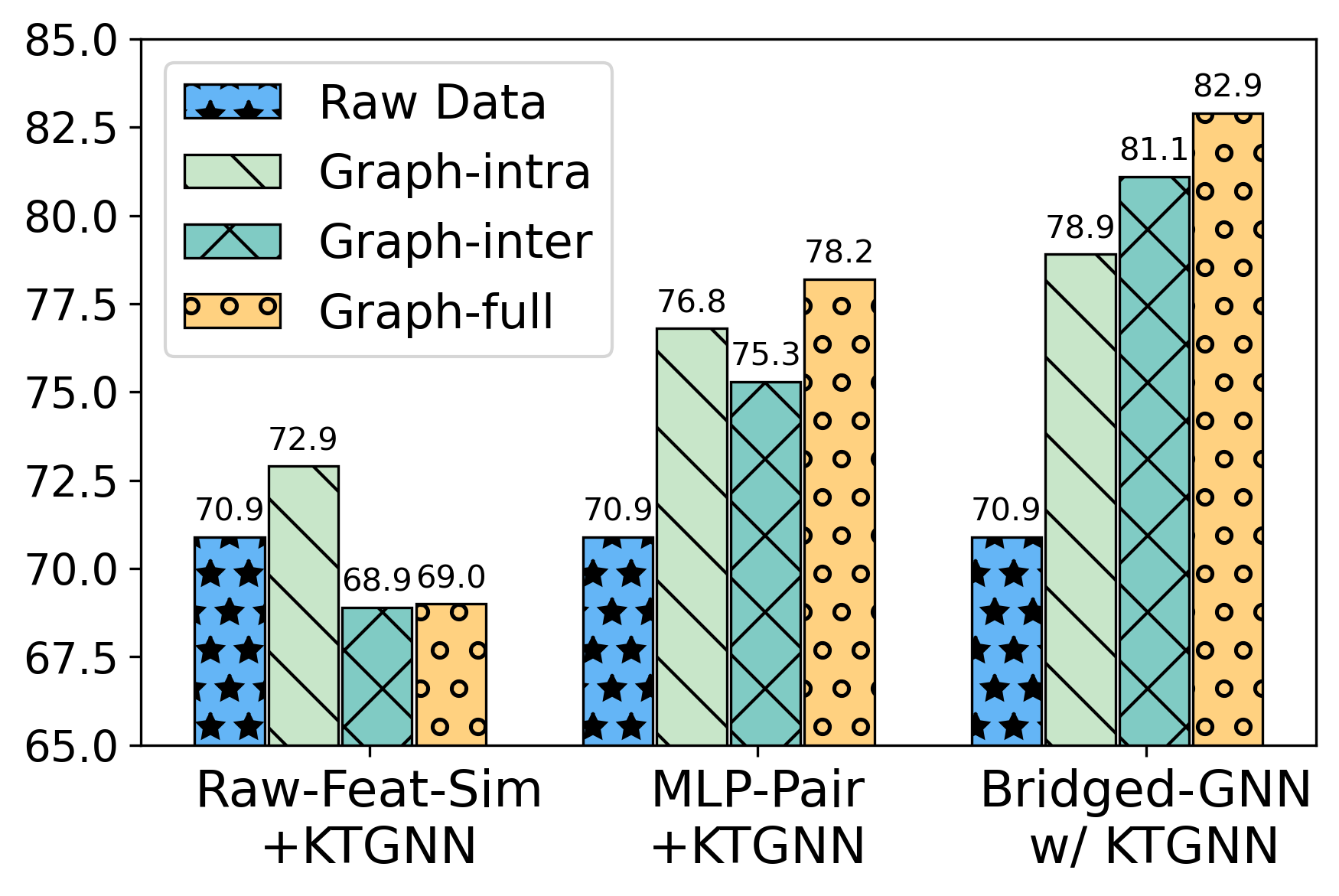
(a) $\text{Twitter}_{UD}$

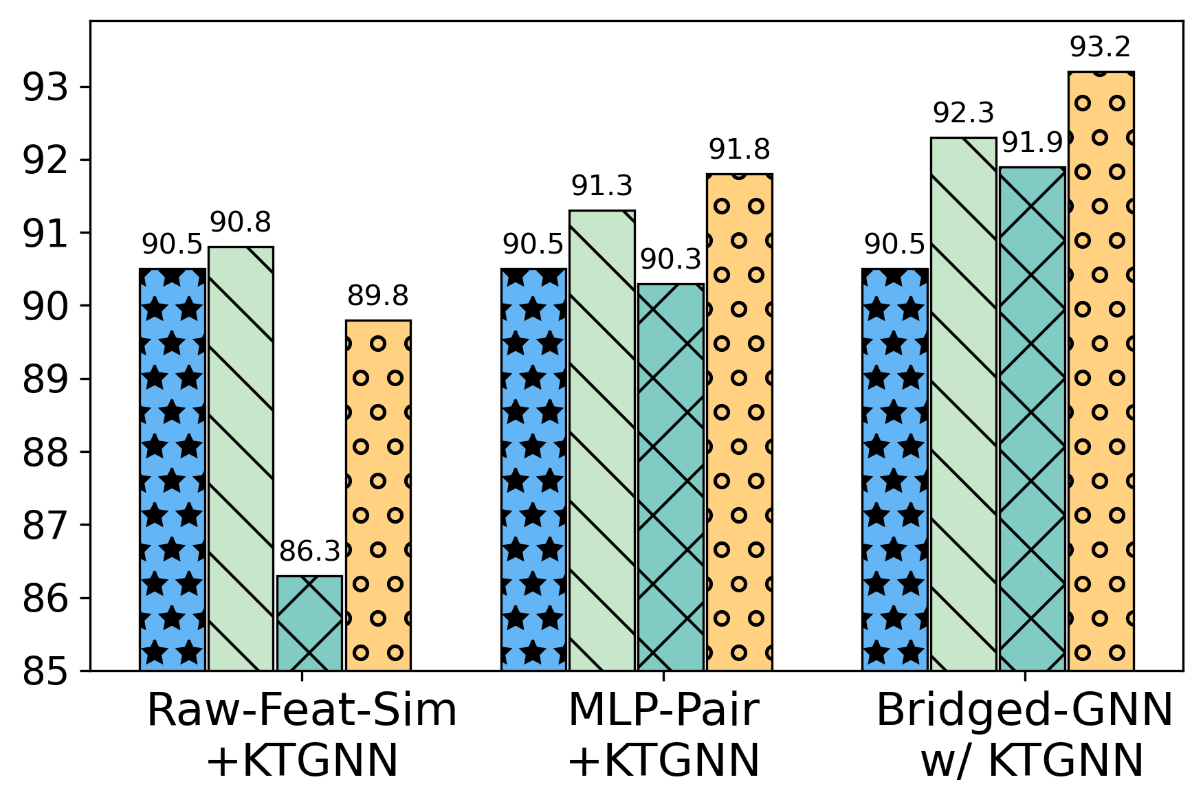
(b) Office31 (A$\rightarrow$D)

Figure 8. Ablation study of Bridged-Graphs with different components, including (1) Raw Data (un-relational) without edges, (2) Graph-intra with only intra-domain edges, (3) Graph-inter with only inter-domain edges, (4) Graph-full with both intra-domain and inter-domain edges. Y-axis denotes the performance of KTGNN.

Table 5. Ablation study by replacing AKR module in $\text{Bridged-GNN}_{\text{KTGNN}}$ with other similarity learners. We evaluate their performance of intra-domain/inter-domain sample-pair classification and target node classification on Bridged-Graphs (denoted by ”NC on Bridged-Graph”).

Replace of AKR	F1-macro@	$\text{Twitter}_{UD}$	Office31 (A$\rightarrow$D)
Raw Feature Similarity	Intra-domain Pair	$47.40$$\pm 0.61$	$76.72$$\pm 0.24$
	Inter-domain Pair	38.28$\pm 0.11$	60.45$\pm 0.23$
	NC on Bridged-Graph	69.01$\pm 0.56$	89.83$\pm 0.55$
Point-wise DNN Classifier	Intra-domain Pair	65.49$\pm 1.83$	87.56$\pm 0.76$
	Inter-domain Pair	60.38$\pm 1.21$	81.32$\pm 0.59$
	NC on Bridged-Graph	71.60$\pm 0.87$	91.03$\pm 0.93$
Pair-wise DNN Classifier	Intra-domain Pair	72.65$\pm 0.98$	92.89$\pm 0.55$
	Inter-domain Pair	70.07$\pm 1.09$	92.66$\pm 0.67$
	NC on Bridged-Graph	78.15$\pm 0.68$	91.89$\pm 0.53$
AKR of Bridged-GNN	Intra-domain Pair	$\mathbf{80.76}$$\mathbf{\pm 1.63}$	$\mathbf{96.09}$$\mathbf{\pm 0.72}$
	Inter-domain Pair	$\bm{78.13}$$\bm{\pm 1.28}$	$\bm{95.41}$$\bm{\pm 0.71}$
	NC on Bridged-Graph	$\mathbf{82.85}$$\mathbf{\pm 0.76}$	$\bm{93.17}$$\bm{\pm 0.39}$

4.4. Ablation Study

We dive into the mechanisms of Bridged-GNN by ablation studies.

4.4.1. Effects of Adaptive Knowledge Retrieval (AKR) module

We conduct ablation studies on the AKR module of Bridged-GNN by comparing our AKR module with other traditional methods of learning sample-pair similarity (Ding et al., 2018; Chen et al., 2021; Wu et al., 2023a), and we evaluate their F1-score of classifying whether pairs of samples belong to the same class or not. As shown in Table 5, Raw Feature Similarity denotes calculating the pair-wise similarity with the raw features. Point-wise DNN Classifier means we directly train a classifier to classify each sample and then calculate the pair-wise similarity with the sample logits (output of the last layer). Pair-wise DNN Classifier means we directly train a DNN-based binary classifier to classify a pair of samples whether they belong to the same class. As shown in Table 5, our AKR module can always gain the best performance on pair-wise classification and node classification on Bridged-Graph.

4.4.2. Effects of Intra-domain/Inter-domain Connections

As shown in Fig. 8, we also validate the effects of intra-domain/inter-domain connections when constructing Bridged-Graphs with the retrieved knowledge (top-K beneficial samples). The results show that the inter-domain connections establishes the bridge for knowledge transfer from the source domain to the target domain, while the intra-domain connections further enlarge the scope and effects of knowledge transfer.

4.5. Hyperparameter Sensitivity Analysis

We analyze the effects of an important hyperparameter K which controls the edge density of the Bridged-Graph. K achieves the trade-off between the quantity and quality of knowledge transfer, i.e., a larger K leads to a larger quantity of knowledge transfer, while the quality of the transferred knowledge is lower. Fig. 9 shows the final classification results of Bridged-GNN with different values of K (X-axis in Fig. 9). By replacing the AKR module in Bridged-GNN with other similarity learners (see Sec. 4.4.1), we observe that the full Bridged-GNN model can always achieve the best performance, and the results of our model are more robust as K increases.

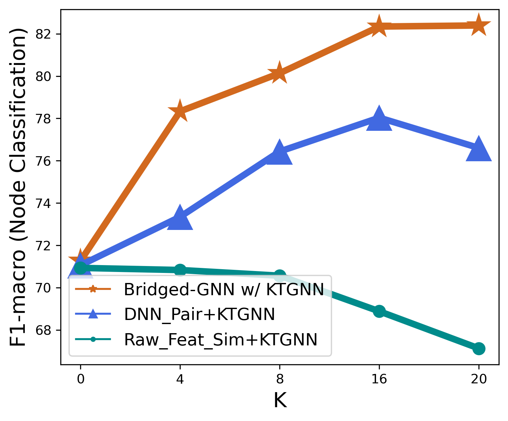
(a) $\text{Twitter}_{UD}$

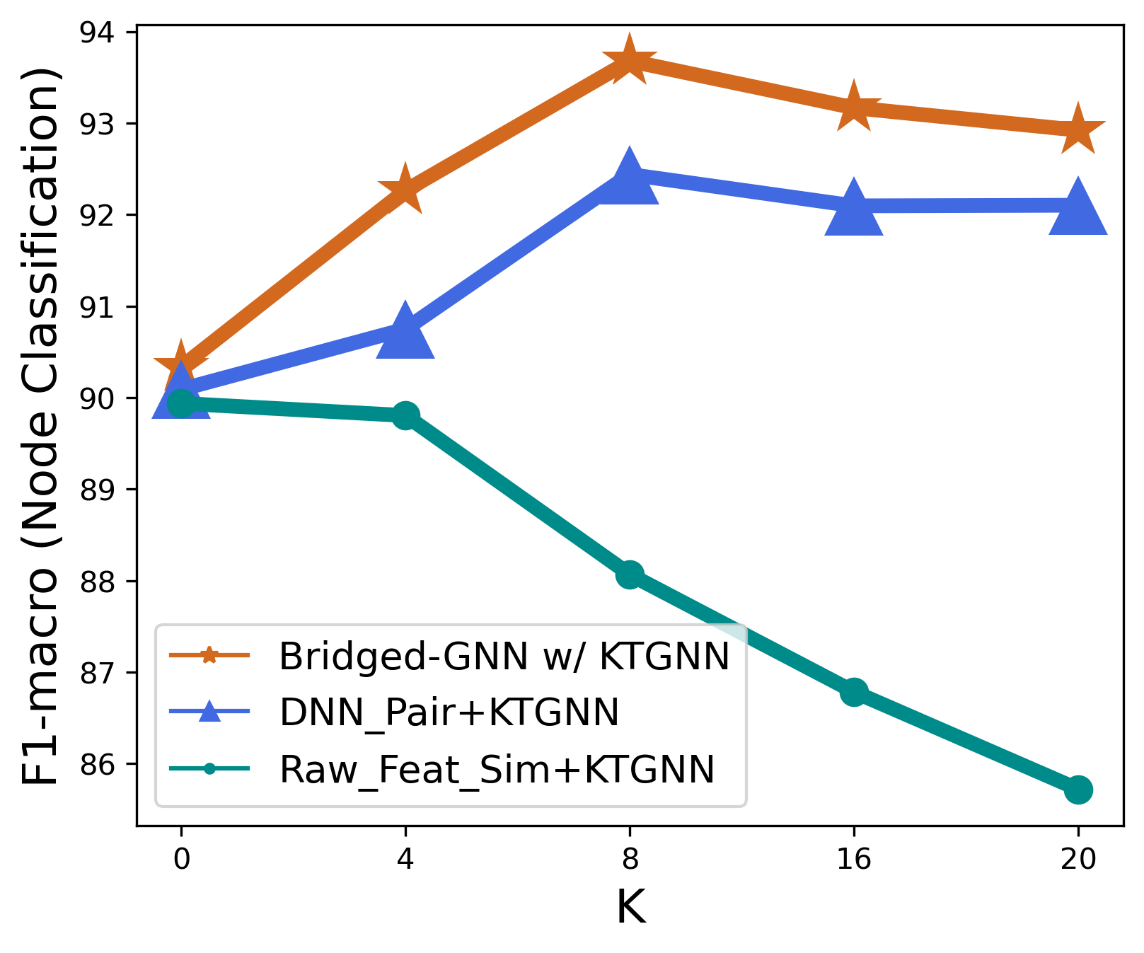
(b) Office31 (A$\rightarrow$D)

Figure 9. Analysis on hyperparameter K, which denotes the number of retrieved knowledgeable nodes for each target node and controls the density of the Bridged-Graph.

5. Related Works

Transfer learning is the mainstream framework of implementing knowledge transfer to alleviate data-hungry. Domain Adaptation (DA), as the representative transfer learning branch, best matches the topic of knowledge transfer in this paper and can be broadly divided into methods with shallow and deep architectures. Shallow DA methods (Gretton et al., 2009; Jhuo et al., 2012) mainly utilize feature-based or instance-reweight-based strategies to minimize the inter-domain distribution distance measured by some metrics (e.g., MMD (Gretton et al., 2006), CORAL (Sun et al., 2017)). Deep DA methods (Hu et al., 2023; Cao et al., 2022; Kang et al., 2023; Hu, 2023; Howard et al., 2022; Su et al., 2022; Yue et al., 2022; Jin et al., 2021) use neural networks to learn shared or separated encoders for both source and target domains, while eliminating the domain gap. However, these methods usually learn a shared posterior distribution between domains and require a relatively closer inter-domain divergence, thus having severe limitations. Traditional DA methods usually refer to unsupervised DA (UDA), while recent studies (Feng et al., 2021; Saito et al., 2019; Wilson and Cook, 2020; Yoon et al., 2022) prove that UDA has significant defects in substantial domain-shift scenarios and propose to gain better performance via semi-supervised DA.

Graph Neural Networks (GNNs) have gained powerful performance on modeling graph data. Existing mainstream GNNs (Xu et al., 2021, 2023; Bi et al., 2023a; Chen et al., 2023; Lin et al., 2014; Xu et al., 2019; Lin et al., 2020; Guo et al., 2022; Gopalakrishnan, 2023) follow the message-passing framework, where node representations are updated based on features aggregated from neighbors. However, most of the existing GNNs are built on the IID hypothesis, i.e., all samples belong to the same data distribution. And the IID hypothesis is hard to be satisfied in many real scenarios, making the model performance degrade significantly. Recently, some GNNs for OOD scenarios (Zhao et al., 2023; Sadeghi et al., 2021; Kang et al., 2022; Huang et al., 2019; Zhang et al., 2023, 2023; Huang et al., 2022) have been designed, and studies (Liu et al., 2021; Bi et al., 2023b; Guo et al., 2023b; Wu et al., 2022b) prove that GNNs can complete inter-domain knowledge transfer on graphs well. However, they strictly rely on high-quality graph structures and cannot be applied to non-graph ($UD$) and cross-graph ($RD_{intra}$) scenarios.

6. Conclusion

In this paper, we redefine the paradigm of knowledge transfer by Knowledge Bridge Learning (KBL) to solve the data-hungry problem. Compared with the existing transfer learning paradigm with strong assumptions, KBL learns a knowledge-enhanced posterior distribution of the target domain by defining the scope of knowledge transfer first and then transferring knowledge with GNNs. Correspondingly, we propose a novel Bridged-GNN model under the paradigm of KBL to conduct sample-wise knowledge transfer in both un-relational and relational data-hungry scenarios. Comprehensive experiments demonstrate that Bridged-GNN under KBL paradigm outperforms existing methods by a large margin.

- (1)
- Bashardoust et al. (2023) Ashkan Bashardoust, Sorelle Friedler, Carlos Scheidegger, Blair D Sullivan, and Suresh Venkatasubramanian. 2023. Reducing Access Disparities in Networks using Edge Augmentation. In Proceedings of the 2023 ACM Conference on Fairness, Accountability, and Transparency. 1635–1651.
- Begga et al. (2023) Ahmed Begga, Francisco Escolano, Miguel Angel Lozano, and Edwin R Hancock. 2023. Diffusion-Jump GNNs: Homophiliation via Learnable Metric Filters. arXiv preprint arXiv:2306.16976 (2023).
- Bi et al. (2022a) Wendong Bi, Lun Du, Qiang Fu, Yanlin Wang, Shi Han, and Dongmei Zhang. 2022a. Make heterophily graphs better fit gnn: A graph rewiring approach. arXiv preprint arXiv:2209.08264 (2022).
- Bi et al. (2023a) Wendong Bi, Lun Du, Qiang Fu, Yanlin Wang, Shi Han, and Dongmei Zhang. 2023a. MM-GNN: Mix-Moment Graph Neural Network towards Modeling Neighborhood Feature Distribution. In Proceedings of the Sixteenth ACM International Conference on Web Search and Data Mining. 132–140.
- Bi et al. (2022b) Wendong Bi, Bingbing Xu, Xiaoqian Sun, Zidong Wang, Huawei Shen, and Xueqi Cheng. 2022b. Company-as-Tribe: Company Financial Risk Assessment on Tribe-Style Graph with Hierarchical Graph Neural Networks. In Proceedings of the 28th ACM SIGKDD Conference on Knowledge Discovery and Data Mining. 2712–2720.
- Bi et al. (2023b) Wendong Bi, Bingbing Xu, Xiaoqian Sun, Li Xu, Huawei Shen, and Xueqi Cheng. 2023b. Predicting the Silent Majority on Graphs: Knowledge Transferable Graph Neural Network. arXiv preprint arXiv:2302.00873 (2023).
- Cai et al. (2021) Ruichu Cai, Fengzhu Wu, Zijian Li, Pengfei Wei, Lingling Yi, and Kun Zhang. 2021. Graph domain adaptation: A generative view. arXiv preprint arXiv:2106.07482 (2021).
- Cao et al. (2022) Jiangxia Cao, Xin Cong, Jiawei Sheng, Tingwen Liu, and Bin Wang. 2022. Contrastive Cross-Domain Sequential Recommendation. In Proceedings of the 31st ACM International Conference on Information & Knowledge Management. 138–147.
- Chen et al. (2009) Bo Chen, Wai Lam, Ivor Tsang, and Tak-Lam Wong. 2009. Extracting discriminative concepts for domain adaptation in text mining. In Proceedings of the 15th ACM SIGKDD international conference on Knowledge discovery and data mining. 179–188.
- Chen et al. (2021) Junjie Chen, Li Niu, Liu Liu, and Liqing Zhang. 2021. Weak-shot fine-grained classification via similarity transfer. Advances in Neural Information Processing Systems 34 (2021), 7306–7318.
- Chen et al. (2020) Ming Chen, Zhewei Wei, Zengfeng Huang, Bolin Ding, and Yaliang Li. 2020. Simple and deep graph convolutional networks. In International Conference on Machine Learning. PMLR, 1725–1735.
- Chen et al. (2023) Yong Chen, Xiao-Zhu Xie, Wei Weng, and Yi-Fan He. 2023. Multi-Order-Content-Based Adaptive Graph Attention Network for Graph Node Classification. Symmetry 15, 5 (2023), 1036.
- Ding et al. (2018) Zhengming Ding, Sheng Li, Ming Shao, and Yun Fu. 2018. Graph adaptive knowledge transfer for unsupervised domain adaptation. In Proceedings of the European Conference on Computer Vision (ECCV). 37–52.
- Duval and Malliaros (2022) Alexandre Duval and Fragkiskos Malliaros. 2022. Higher-order clustering and pooling for graph neural networks. In Proceedings of the 31st ACM International Conference on Information & Knowledge Management. 426–435.
- Feng et al. (2021) Cheng Feng, Chaoliang Zhong, Jie Wang, Jun Sun, and Yasuto Yokota. 2021. CANN: Coupled Approximation Neural Network for Partial Domain Adaptation. In Proceedings of the 30th ACM International Conference on Information & Knowledge Management. 464–473.
- Ganin and Lempitsky (2015) Yaroslav Ganin and Victor Lempitsky. 2015. Unsupervised domain adaptation by backpropagation. In International conference on machine learning. PMLR, 1180–1189.
- Gopalakrishnan (2023) Atul Anand Gopalakrishnan. 2023. Graph Augmentation Using Spectral Moments. Ph. D. Dissertation. Syracuse University.
- Gretton et al. (2006) Arthur Gretton, Karsten Borgwardt, Malte Rasch, Bernhard Schölkopf, and Alex Smola. 2006. A kernel method for the two-sample-problem. Advances in neural information processing systems 19 (2006).
- Gretton et al. (2009) Arthur Gretton, Alex Smola, Jiayuan Huang, Marcel Schmittfull, Karsten Borgwardt, and Bernhard Schölkopf. 2009. Covariate shift by kernel mean matching. Dataset shift in machine learning 3, 4 (2009), 5.
- Gui et al. (2022) Shurui Gui, Xiner Li, Limei Wang, and Shuiwang Ji. 2022. GOOD: A Graph Out-of-Distribution Benchmark. arXiv preprint arXiv:2206.08452 (2022).
- Guo et al. (2023a) Jiayan Guo, Lun Du, Wendong Bi, Qiang Fu, Xiaojun Ma, Xu Chen, Shi Han, Dongmei Zhang, and Yan Zhang. 2023a. Homophily-oriented Heterogeneous Graph Rewiring. In Proceedings of the ACM Web Conference 2023. 511–522.
- Guo et al. (2023b) Jiayan Guo, Lun Du, Xu Chen, Xiaojun Ma, Qiang Fu, Shi Han, Dongmei Zhang, and Yan Zhang. 2023b. On Manipulating Signals of User-Item Graph: A Jacobi Polynomial-based Graph Collaborative Filtering. arXiv preprint arXiv:2306.03624 (2023).
- Guo et al. (2022) Jiayan Guo, Yaming Yang, Xiangchen Song, Yuan Zhang, Yujing Wang, Jing Bai, and Yan Zhang. 2022. Learning Multi-granularity User Intent Unit for Session-based Recommendation. In Proceedings of the 15’th ACM International Conference on Web Search and Data Mining WSDM’22.
- Hamilton et al. (2017) William L Hamilton, Rex Ying, and Jure Leskovec. 2017. Inductive representation learning on large graphs. In Proceedings of the 31st International Conference on Neural Information Processing Systems. 1025–1035.
- Howard et al. (2022) Phillip Howard, Arden Ma, Vasudev Lal, Ana Paula Simoes, Daniel Korat, Oren Pereg, Moshe Wasserblat, and Gadi Singer. 2022. Cross-Domain Aspect Extraction using Transformers Augmented with Knowledge Graphs. In Proceedings of the 31st ACM International Conference on Information & Knowledge Management. 780–790.
- Hu (2023) Jing Hu. 2023. Intelligent Financial Decision Support System Using Artificial Intelligence. In 2023 International Conference on Applied Intelligence and Sustainable Computing (ICAISC). IEEE, 1–6.
- Hu et al. (2023) Xiyang Hu, Yan Huang, Beibei Li, and Tian Lu. 2023. Inclusive FinTech Lending via Contrastive Learning and Domain Adaptation. arXiv preprint arXiv:2305.05827 (2023).
- Huang et al. (2022) Tiancheng Huang, Donglin Wang, Yuan Fang, and Zhengyu Chen. 2022. End-to-End Open-Set Semi-Supervised Node Classification with Out-of-Distribution Detection. IJCAI (2022).
- Huang et al. (2019) Ziling Huang, Zheng Wang, Wei Hu, Chia-Wen Lin, and Shin’ichi Satoh. 2019. DoT-GNN: Domain-transferred graph neural network for group re-identification. In Proceedings of the 27th ACM International Conference on Multimedia. 1888–1896.
- Jhuo et al. (2012) I-Hong Jhuo, Dong Liu, DT Lee, and Shih-Fu Chang. 2012. Robust visual domain adaptation with low-rank reconstruction. In 2012 IEEE conference on computer vision and pattern recognition. IEEE, 2168–2175.
- Jin et al. (2020) Di Jin, Zhijing Jin, Joey Tianyi Zhou, and Peter Szolovits. 2020. A simple baseline to semi-supervised domain adaptation for machine translation. arXiv preprint arXiv:2001.08140 (2020).
- Jin et al. (2021) Di Jin, Bunyamin Sisman, Hao Wei, Xin Luna Dong, and Danai Koutra. 2021. Deep transfer learning for multi-source entity linkage via domain adaptation. arXiv preprint arXiv:2110.14509 (2021).
- Kang et al. (2022) Qiyu Kang, Kai Zhao, Yang Song, Sijie Wang, and Wee Peng Tay. 2022. NEURAL HAMILTONIAN FLOWS IN GRAPH NEURAL NETWORKS. (2022).
- Kang et al. (2023) Qiyu Kang, Kai Zhao, Yang Song, Sijie Wang, and Wee Peng Tay. 2023. Node Embedding from Neural Hamiltonian Orbits in Graph Neural Networks. arXiv preprint arXiv:2305.18965 (2023).
- Kim and Kim (2020) Taekyung Kim and Changick Kim. 2020. Attract, perturb, and explore: Learning a feature alignment network for semi-supervised domain adaptation. In Computer Vision–ECCV 2020: 16th European Conference, Glasgow, UK, August 23–28, 2020, Proceedings, Part XIV 16. Springer, 591–607.
- Kipf and Welling (2016) Thomas N Kipf and Max Welling. 2016. Semi-supervised classification with graph convolutional networks. arXiv preprint arXiv:1609.02907 (2016).
- Li et al. (2023) Yixia Li, Rong Xiang, Yanlin Song, and Jing Li. 2023. UniPoll: A Unified Social Media Poll Generation Framework via Multi-Objective Optimization. arXiv preprint arXiv:2306.06851 (2023).
- Liang et al. (2022a) Ke Liang, Yue Liu, Sihang Zhou, Xinwang Liu, and Wenxuan Tu. 2022a. Relational symmetry based knowledge graph contrastive learning. arXiv preprint arXiv:2211.10738 (2022).
- Liang et al. (2022b) Ke Liang, Lingyuan Meng, Meng Liu, Yue Liu, Wenxuan Tu, Siwei Wang, Sihang Zhou, Xinwang Liu, and Fuchun Sun. 2022b. Reasoning over Different Types of Knowledge Graphs: Static, Temporal and Multi-Modal. https://doi.org/10.48550/ARXIV.2212.05767
- Lin et al. (2020) Wenqing Lin, Feng He, Faqiang Zhang, Xu Cheng, and Hongyun Cai. 2020. Initialization for network embedding: A graph partition approach. In Proceedings of the 13th International Conference on Web Search and Data Mining. 367–374.
- Lin et al. (2014) Wenqing Lin, Xiaokui Xiao, and Gabriel Ghinita. 2014. Large-scale frequent subgraph mining in mapreduce. In 2014 IEEE 30th International Conference on Data Engineering. IEEE, 844–855.
- Liu et al. (2021) Ziqi Liu, Yue Shen, Xiaocheng Cheng, Qiang Li, Jianping Wei, Zhiqiang Zhang, Dong Wang, Xiaodong Zeng, Jinjie Gu, and Jun Zhou. 2021. Learning Representations of Inactive Users: A Cross Domain Approach with Graph Neural Networks. In Proceedings of the 30th ACM International Conference on Information & Knowledge Management. 3278–3282.
- Long et al. (2015) Mingsheng Long, Yue Cao, Jianmin Wang, and Michael Jordan. 2015. Learning transferable features with deep adaptation networks. In International conference on machine learning. PMLR, 97–105.
- Long et al. (2018) Mingsheng Long, Zhangjie Cao, Jianmin Wang, and Michael I Jordan. 2018. Conditional adversarial domain adaptation. Advances in neural information processing systems 31 (2018).
- Long et al. (2013) Mingsheng Long, Jianmin Wang, Guiguang Ding, Jiaguang Sun, and Philip S Yu. 2013. Transfer feature learning with joint distribution adaptation. In Proceedings of the IEEE international conference on computer vision. 2200–2207.
- Long et al. (2017) Mingsheng Long, Han Zhu, Jianmin Wang, and Michael I Jordan. 2017. Deep transfer learning with joint adaptation networks. In International conference on machine learning. PMLR, 2208–2217.
- Pan and Kang (2023) Erlin Pan and Zhao Kang. 2023. Beyond Homophily: Reconstructing Structure for Graph-agnostic Clustering. arXiv preprint arXiv:2305.02931 (2023).
- Ren et al. (2022) Jiaqian Ren, Lei Jiang, Hao Peng, Yuwei Cao, Jia Wu, Philip S Yu, and Lifang He. 2022. From known to unknown: quality-aware self-improving graph neural network for open set social event detection. arXiv preprint arXiv:2208.06973 (2022).
- Sadeghi et al. (2021) Alireza Sadeghi, Meng Ma, Bingcong Li, and Georgios B Giannakis. 2021. Distributionally Robust Semi-Supervised Learning Over Graphs. arXiv preprint arXiv:2110.10582 (2021).
- Saito et al. (2019) Kuniaki Saito, Donghyun Kim, Stan Sclaroff, Trevor Darrell, and Kate Saenko. 2019. Semi-supervised domain adaptation via minimax entropy. In Proceedings of the IEEE/CVF international conference on computer vision. 8050–8058.
- Song and Wang (2022) Yu Song and Donglin Wang. 2022. Learning on Graphs with Out-of-Distribution Nodes. In Proceedings of the 28th ACM SIGKDD Conference on Knowledge Discovery and Data Mining. 1635–1645.
- Su et al. (2022) Hongzu Su, Yifei Zhang, Xuejiao Yang, Hua Hua, Shuangyang Wang, and Jingjing Li. 2022. Cross-domain Recommendation via Adversarial Adaptation. In Proceedings of the 31st ACM International Conference on Information & Knowledge Management. 1808–1817.
- Sun et al. (2017) Baochen Sun, Jiashi Feng, and Kate Saenko. 2017. Correlation alignment for unsupervised domain adaptation. Domain adaptation in computer vision applications (2017), 153–171.
- Sun et al. (2014) Xiaoqian Sun, Xueqi Cheng, and Huawei Shen. 2014. Trading network predicts stock price. Scientific Reports 4, 1 (2014), 313–317.
- Sun et al. (2011) Xiaoqian Sun, Xueqi Cheng, Huawei Shen, and Zhaoyang Wang. 2011. Distinguishing manipulated stocks via trading network analysis. Physica A 390 (2011), 3427–3434.
- Traud et al. (2012) Amanda L Traud, Peter J Mucha, and Mason A Porter. 2012. Social structure of Facebook networks. Physica A: Statistical Mechanics and its Applications 391, 16 (2012), 4165–4180.
- Veličković et al. (2017) Petar Veličković, Guillem Cucurull, Arantxa Casanova, Adriana Romero, Pietro Lio, and Yoshua Bengio. 2017. Graph attention networks. arXiv preprint arXiv:1710.10903 (2017).
- Wang et al. (2022) Xiang Wang, An Zhang, Xia Hu, Fuli Feng, Xiangnan He, Tat-Seng Chua, et al. 2022. Deconfounding to Explanation Evaluation in Graph Neural Networks. arXiv preprint arXiv:2201.08802 (2022).
- Wilson and Cook (2020) Garrett Wilson and Diane J Cook. 2020. A survey of unsupervised deep domain adaptation. ACM Transactions on Intelligent Systems and Technology (TIST) 11, 5 (2020), 1–46.
- Wu et al. (2023a) First Jianqiu Wu, Second Hongyang Chen, Third Minhao Cheng, and Fourth Haoyi Xiong. 2023a. CurvAGN: Curvature-based Adaptive Graph Neural Networks for Predicting Protein-Ligand Binding Affinity. (2023).
- Wu et al. (2023b) Qitian Wu, Yiting Chen, Chenxiao Yang, and Junchi Yan. 2023b. Energy-based Out-of-Distribution Detection for Graph Neural Networks. In International Conference on Learning Representations.
- Wu et al. (2022b) Qitian Wu, Hengrui Zhang, Junchi Yan, and David Wipf. 2022b. Handling distribution shifts on graphs: An invariance perspective. arXiv preprint arXiv:2202.02466 (2022).
- Wu et al. (2022a) Ying-Xin Wu, Xiang Wang, An Zhang, Xiangnan He, and Tat-Seng Chua. 2022a. Discovering invariant rationales for graph neural networks. arXiv preprint arXiv:2201.12872 (2022).
- Xiao et al. (2020) Zhiping Xiao, Weiping Song, Haoyan Xu, Zhicheng Ren, and Yizhou Sun. 2020. TIMME: Twitter ideology-detection via multi-task multi-relational embedding. In Proceedings of the 26th ACM SIGKDD International Conference on Knowledge Discovery & Data Mining. 2258–2268.
- Xu et al. (2023) Bingbing Xu, Yang Li, Qi Cao, and Huawei Shen. 2023. Simple Multi-view Can Bring Powerful Graph Neural Network. In Companion Proceedings of the ACM Web Conference 2023. 322–325.
- Xu et al. (2019) Bingbing Xu, Huawei Shen, Qi Cao, Yunqi Qiu, and Xueqi Cheng. 2019. Graph wavelet neural network. arXiv preprint arXiv:1904.07785 (2019).
- Xu et al. (2021) Bingbing Xu, Huawei Shen, Bingjie Sun, Rong An, Qi Cao, and Xueqi Cheng. 2021. Towards consumer loan fraud detection: Graph neural networks with role-constrained conditional random field.
- Yang et al. (2023) Han Yang, Junyuan Fang, Jiajing Wu, and Zibin Zheng. 2023. Both Homophily and Heterophily Matter: Bi-path Aware Graph Neural Network for Ethereum Account Classification. IEEE Journal on Emerging and Selected Topics in Circuits and Systems (2023).
- Yoon et al. (2022) Jeongbeen Yoon, Dahyun Kang, and Minsu Cho. 2022. Semi-supervised domain adaptation via sample-to-sample self-distillation. In Proceedings of the IEEE/CVF Winter Conference on Applications of Computer Vision. 1978–1987.
- Yue et al. (2022) Zhenrui Yue, Huimin Zeng, Ziyi Kou, Lanyu Shang, and Dong Wang. 2022. Contrastive domain adaptation for early misinformation detection: A case study on covid-19. In Proceedings of the 31st ACM International Conference on Information & Knowledge Management. 2423–2433.
- Zhang et al. (2023) Yanci Zhang, Yutong Lu, Haitao Mao, Jiawei Huang, Cien Zhang, Xinyi Li, and Rui Dai. 2023. Company Competition Graph. arXiv preprint arXiv:2304.00323 (2023).
- Zhang et al. (2019) Yaping Zhang, Shuai Nie, Wenju Liu, Xing Xu, Dongxiang Zhang, and Heng Tao Shen. 2019. Sequence-to-sequence domain adaptation network for robust text image recognition. In Proceedings of the IEEE/CVF conference on computer vision and pattern recognition. 2740–2749.
- Zhao et al. (2023) Wentao Zhao, Qitian Wu, Chenxiao Yang, and Junchi Yan. 2023. GraphGLOW: Universal and Generalizable Structure Learning for Graph Neural Networks. arXiv preprint arXiv:2306.11264 (2023).