STAR-RIS Aided MISO SWIPT-NOMA System with Energy Buffer: Performance Analysis and Optimization

Abstract

In this paper, we propose a simultaneous transmitting and reflecting reconfigurable intelligent surface (STAR-RIS) and energy buffer aided multiple-input single-output (MISO) simultaneous wireless information and power transfer (SWIPT) non-orthogonal multiple access (NOMA) system, which consists of a STAR-RIS, an access point (AP), and reflection users and transmission users with energy buffers. In the proposed system, the multi-antenna AP can transmit information and energy to several single-antenna reflection and transmission users simultaneously in a NOMA fashion, where the power transfer and information transmission states of the users are modeled using Markov chains. The reflection and transmission users harvest and store the energy in energy buffers as additional power supplies. The power outage probability, information outage probability, sum throughput, and joint outage probability closed-form expressions of the proposed system are derived over Nakagami-$m$ fading channels, which are validated via simulations. Results demonstrate that the proposed system achieves better performance in comparison to the STAR-RIS aided MISO SWIPT-NOMA buffer-less, conventional RIS and energy buffer aided MISO SWIPT-NOMA, and STAR-RIS and energy buffer aided MISO SWIPT-time-division multiple access (TDMA) systems. Furthermore, a particle swarm optimization based power allocation (PSO-PA) algorithm is designed to maximize the sum throughput with a constraint on the joint outage probability. Simulation results illustrate that the proposed PSO-PA algorithm can achieve an improved sum throughput performance of the proposed system.

I Introduction

Internet of Things (IoT) has been considered as one of the key and enabling paradigms for a plethora of applications in healthcare, smart cities, and smart homes[1]. In the IoT era, various low-power wireless sensor devices are connected to the network and interact with each other[2]. However, the ever-increasing of wireless electronics inevitably impose challenges on power supply of devices and massive multiple access, owing to the limited battery lifespans of devices and scarce spectral resources[3].

Regarding the limited battery challenge although several energy harvesting methods, such as solar and wind energy harvesting, can capture energy from environment, their availability is out of control[4]. To prolong the operational lifetime of the energy-constrained and low-power devices, simultaneous wireless information and power transfer (SWIPT) has been proposed, which offers a controllable way to charge devices by utilizing the ubiquitous radio-frequency (RF) signals[5]. SWIPT enables devices to receive power and information simultaneously. In addition, to tackle the aforementioned massive connectivity issue, non-orthogonal multiple access (NOMA) technology has been proposed[6]. In contrast to orthogonal multiple access (OMA), NOMA allows multiple users to share the same time-frequency resource, therefore providing better spectrum efficiency[7]. Recent studies have combined NOMA and SWIPT to prolong the lifetime of energy-constrained IoT networks and support massive connectivity[8, 9, 10, 11]. In [8], a time switching based SWIPT-NOMA system was proposed with joint power allocation and time switching control for energy efficiency optimization. In [9], a downlink coordinated multipoint SWIPT-NOMA network was proposed. To further improve the performance, multiple antennas have been introduced into the SWIPT-NOMA system. In [10], a multiuser multiple-input single-output (MISO) SWIPT-NOMA network was studied, where a novel hybrid user pairing scheme was proposed. In [11], a millimeter-wave multiple-input multiple-output (MIMO) SWIPT-NOMA system was investigated. The above works assumed that all harvested energy is consumed in one time slot and energy harvesting is performed with the harvest-use (HU) architecture. However, in practice, the harvested energy being small and random, this limits the performance of SWIPT-NOMA systems. Therefore, the energy buffer with the harvest-store-use (HSU) architecture was considered for storing the harvested energy, which can improve the performance of self-sustaining nodes[12, 13, 14]. In [12], a wireless-powered cooperative NOMA relay network was considered, where the relay was provisioned with energy buffer to improve the energy efficiency. In [13], an adaptive multiuser cooperative NOMA scheme was studied, where the near-user was equipped with an energy buffer to harvest energy from the ambiance, thus improving the system throughput. In [14], an MISO wireless-powered NOMA network was investigated, which considers the utilization of a data buffer and an energy storage at sources to achieve both higher sum rate and improved fairness.

Recently, reconfigurable intelligent surfaces (RISs) have received extensive attention from both academia and industry[15], which can bring enhanced spectrum and energy efficiencies[16]. A RIS is composed of massive reflecting elements that are energy efficient and cost effective[17], which has been introduced into SWIPT-NOMA systems for improved system performance. On the one hand, the efficiency of SWIPT highly depends on the existence of a line-of-sight (LoS) link[18] which may be blocked by various obstacles due to long distance transmissions. On the other hand, the far-field user in NOMA may experience poor performance due to path loss. RISs are not only capable of building virtual LoS links when LoS links are blocked[19], but can also bring outstanding performance gains in SWIPT[20]. Hence, tremendous research efforts have been devoted to RIS-aided SWIPT-NOMA systems[21, 22, 23]. A RIS-assisted cooperative SWIPT-NOMA system was investigated in [21, 22], where [21] focused on improving the achievable rate of the strong user with guaranteeing the weak user’s quality of service and [22] is devoted to maximizing the data rate of the cell-edge user. A RIS-aided MISO SWIPT-NOMA system was proposed in [23], which considered a cooperative transmission scheme to improve the performance of cell-edge users. However, in [21, 22, 23], the HU architecture was utilized to harvest energy, where energy harvesting nodes do not buffer the energy for use in future time slots. Moreover, the conventional RIS only reflects the wireless signal to the users, which makes it necessary for the transmitter and receiver to be on the same side.

To overcome the limitation of user distribution in conventional RIS aided systems, the novel concept of simultaneous transmitting and reflecting RIS (STAR-RIS) has been recently proposed [24, 25]. Different from the conventional RIS, STAR-RIS provides full-space service coverage and a more flexible deployment[26], which can not only reflect but also transmit (also known as refract) the incident signal. Specifically, the incident signal on the STAR-RIS is divided into two parts. One part is reflected to the same space as the transmitter, i.e., the reflection space, and the other part is transmitted to the opposite space, i.e., the transmission space[27]. Moreover, three practical protocols of STAR-RIS have been proposed in [27], i.e., time-switching, mode-switching, and energy-splitting. Because the STAR-RIS would divide the incident signal into two portions in the energy-splitting protocol and mode-switching protocol, a multiple access scheme is necessary to distinguish these two parts to decode them successfully [28]. NOMA has been considered to be a promising multiple access technique due to its ability to provide enhanced spectral efficiency and connectivity[29, 30]. Recently, STAR-RIS aided NOMA networks have been investigated in several works[31, 32, 33]. In [31], a STAR-RIS aided NOMA system was investigated to maximize the achievable sum rate. In [32], a STAR-RIS assisted downlink MISO-NOMA network was considered for maximizing the system energy efficiency. In [33], a STAR-RIS assisted downlink MIMO-NOMA network was considered to investigate the energy-efficient resource allocation. To study the potential benefits of deploying STAR-RIS in wireless-powered transmission, there have been some initial works on STAR-RIS aided wireless-powered systems[34, 35, 36, 37]. In [34], a STAR-RIS aided wireless-powered mobile edge computing system was investigated. In [35], a STAR-RIS assisted wireless-powered IoT network was proposed, which adopts the time division multiple access (TDMA) scheme. In [36], a STAR-RIS aided wireless-powered NOMA system was investigated, where the time-switching protocol and energy-splitting protocol of STAR-RIS are utilized to improve the sum throughput. In [37], a STAR-RIS aided SWIPT system was proposed, where STAR-RIS employs the time-switching protocol. However, in [34, 35, 36, 37], only single-antenna access points (APs) with the HU architecture were considered.

In light of the aforementioned motivations, we propose a STAR-RIS and energy buffer aided MISO SWIPT-NOMA system in this paper. The HSU architecture for users with energy buffers is adopted to achieve energy management, thus ensuring better performance. The main contributions of this paper can be summarized as follows:

• We consider a STAR-RIS and energy buffer aided MISO SWIPT-NOMA system, where a multi-antenna AP transmits the superimposed signals to several single-antenna users via the direct link and reflection/transmission links assisted by STAR-RIS. Successive interference cancellation (SIC) is considered for information decoding at users. Moreover, the reflection and transmission users are equipped with energy buffers to enhance the system’s sustainability, where the power transfer and information transmission states are modeled using Markov chains. In this system, the sustainability is studied from the perspectives of both energy acquisition and consumption.

• By exploiting the moment-matching approach, the proposed system’s power outage probability, information outage probability, and sum throughput performances are derived in closed form over Nakagami-$m$ fading channels. The power and information outage probabilities are combined into a closed-form joint outage probability. Simulations are carried out to verify the accuracy of the theoretical analysis and demonstrate that the proposed system offers improved performance compared to baseline schemes.

• To achieve the maximization of sum throughput while ensuring a certain joint outage probability for users, a low-complexity particle swarm optimization-based power allocation (PSO-PA) algorithm is proposed to find the optimal energy-splitting ratios of the STAR-RIS and the power-splitting factor. Results unveil that the proposed PSO-PA algorithm provides an improved sum throughput performance for the proposed system by jointly optimizing the energy-splitting ratios of the STAR-RIS and the power-splitting factor.

The rest of this paper is organized as follows. In Section II, we introduce the system model. In Section III, we analyze the performance of the proposed system. In Section IV, we propose the resource allocation method. Simulation results and discussions are summarized in Section V. Finally, we conclude the paper in Section VI.

Notations: Matrices and vectors are denoted by uppercase bold and lowercase bold, respectively. ${\mathbb{C}^{M\times 1}}$ denotes the space of $M\times 1$ complex vectors. ${j^{2}}=-1$ and $j$ denotes the imaginary unit. diag($\mathbf{x}$) denotes a diagonal matrix with the elements of vector $\mathbf{x}$ on the main diagonal. The complex Gaussian distribution is denoted by $\mathcal{CN}\left({\mu,{\sigma^{2}}}\right)$ with mean $\mu$ and variance ${{\sigma^{2}}}$. ${K_{\alpha}}\left(\cdot\right)$ denotes the modified Bessel function of the second kind. ${I_{\alpha}}\left(\cdot\right)$ is the $\alpha$-th order Bessel function of the first kind. $\gamma\left({\cdot,\cdot}\right)$ is the upper incomplete Gamma function. $\Gamma\left(\cdot\right)$ is the Gamma function. $\mathrm{E}\left(\cdot\right)$ and $\mathrm{Var}\left(\cdot\right)$ represent the expectation and variance operations, respectively. $\max\left({a,b}\right)$ returns the maximum of $a$ and $b$.

II System Model

This section first describes the proposed system and its signal model, and then presents the energy consumption model.

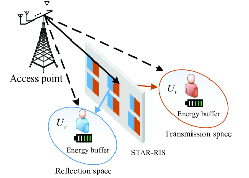
Figure 1: STAR-RIS and energy buffer aided MISO SWIPT-NOMA system.

II-A STAR-RIS and Energy Buffer Aided MISO SWIPT-NOMA System

Fig. 1 illustrates the proposed STAR-RIS and energy buffer aided MISO SWIPT-NOMA system, consisting of an $L$-antenna AP, a STAR-RIS, reflection users, and transmission users. The $L$-antenna AP can communicate with single-antenna reflection users and transmission users with the aid of the STAR-RIS that is composed of $N$ low-cost reflective elements. It is assumed that the direct link from the AP to the user is available. Frequency division multiplexing is applied to serve multiple users. At the AP, the total bandwidth $W$ is divided into $\mathcal{K}$ sub-channels, where each sub-channel can be occupied by at most two users[30]. In addition, we assume that each user can occupy at most one subcarrier. Hence, all reflection and transmission users are divided into $\mathcal{K}$ pairs. For simplicity of presentation and revealing fundamental insights, in this paper, we consider a two-user setup, i.e., one reflection user ${U_{r}}$ and one transmission user ${U_{t}}$. The AP has a fixed energy supply, while ${U_{r}}$ and ${U_{t}}$ are powered by harvested energy due to energy constraints. The AP simultaneously transmits the energy and information to ${U_{r}}$ and ${U_{t}}$ using NOMA. After harvesting the energy, ${U_{r}}$ and ${U_{t}}$ use the harvested energy to power the RF chain and signal processing circuit. The information transmission and energy transfer from the AP to ${U_{k}}$, $k\in\left\{{t,r}\right\}$ are assisted by STAR-RIS in the downlink.

II-B Signal Model

The STAR-RIS works using the energy-splitting protocol, where the AP can simultaneously communicate with users located on opposite sides of the STAR-RIS using NOMA. In the energy-splitting protocol, each element of the STAR-RIS operates simultaneously in transmission and reflection modes, where $\sqrt{{\beta_{r}}},\sqrt{{\beta_{t}}}\in\left[{0,1}\right]$ denote the energy-splitting ratios. $\beta_{r}+\beta_{t}=1$ holds based on the law of energy conservation[30, 41]. Let ${{\bm{\varphi}}_{r}}\buildrel\Delta\over{=}\left[{\sqrt{{\beta_{r}}}{e^{j\varphi_{1}^{r}}},\ldots,\sqrt{{\beta_{r}}}{e^{j\varphi_{N}^{r}}}}\right]$ and ${{\bm{\varphi}}_{t}}\buildrel\Delta\over{=}\left[{\sqrt{{\beta_{t}}}{e^{j\varphi_{1}^{t}}},\ldots,\sqrt{{\beta_{t}}}{e^{j\varphi_{N}^{t}}}}\right]$ denote the STAR-RIS’s reflection and transmission coefficient vectors, where $\varphi_{i}^{r},\varphi_{i}^{t}\in\left[{0,2\pi}\right),i\in\left\{{1,2,\ldots,N}\right\}$ denote the phase-shift adjustments at the $i$-th element.

II-B1 Information transmission

Let ${\mathbf{\tilde{H}}}\in{\mathbb{C}^{N\times L}}$ be the complex channel coefficients matrix, ${\mathbf{\tilde{g}}_{k}}\in{\mathbb{C}^{1\times N}}$ be the complex channel coefficients vector, ${{\bf{\tilde{h}}}_{k}^{0}}\in{\mathbb{C}^{1\times L}}$ be the complex channel coefficients vector of the direct link between the AP and STAR-RIS, the STAR-RIS and ${U_{k}}$, and the AP and ${U_{k}}$. The AP uses NOMA to form a superimposed signal $s=\sqrt{{P_{\text{AP}}}/L}\left({\sqrt{{\alpha_{r}}}{s_{r}}+\sqrt{{\alpha_{t}}}{s_{t}}}\right)$, where ${P_{\text{AP}}}/L$ is the transmit power of each antenna at the AP, ${{\alpha_{r}}}$ and ${{\alpha_{t}}}$ are the transmit power allocation factors for ${U_{r}}$ and ${U_{t}}$ with ${\alpha_{r}}+{\alpha_{t}}=1$, and ${s_{r}}$ and ${s_{t}}$ are the unit-energy information signals of ${U_{r}}$ and ${U_{t}}$, i.e., $\mathrm{E}\left({{{\left|{{s_{r}}}\right|}^{2}}}\right)=\mathrm{E}\left({{{\left|{{s_{t}}}\right|}^{2}}}\right)=1$.

In the proposed system, the power-splitting mode is adopted in the SWIPT, with $\theta$ being the power-splitting factor, which indicates the portion of the received signal used for information decoding. The received signal for information decoding at ${U_{k}}$ can be expressed as

$${y_{k}}=\sqrt{\theta}\left({{\bf{\tilde{h}}}_{{k}}^{{0}}{\bf{w}}+{{{\bf{\tilde{g}}}}_{{k}}}{\rm{diag}}({{\bm{\varphi}}_{{k}}}){\bf{\tilde{H}w}}}\right)s+{n_{k}}$$

$$=\sqrt{\theta{\beta_{k}}}\sum\limits_{\ell=1}^{L}{\left({\tilde{h}_{k,\ell}^{0}{e^{-j{\varpi_{\ell}}}}+\sum\limits_{i=1}^{N}{{{\tilde{h}}_{\ell,i}}{{\tilde{g}}_{k,i}}{e^{j\left({\varphi_{i}^{k}-{\varpi_{\ell}}}\right)}}}}\right)}s+{n_{k}},$$ (1)

where $\mathbf{w}=\left[{{e^{-j{\varpi_{1}}}},\ldots,{e^{-j{\varpi_{L}}}}}\right]$ is the beamforming vector, and ${n_{k}}$ is the additive white Gaussian noise (AWGN) with ${n_{k}}\sim{\cal C}{\cal N}\left({0,{N_{0}}}\right)$.

II-B2 Energy harvesting

At ${U_{k}}$, the harvested energy can be calculated as

$${E_{k}}=\eta\left({1-\theta}\right){\beta_{k}}{\left|{\sum\limits_{\ell=1}^{L}{\left(\begin{array}[]{l}\tilde{h}_{k,\ell}^{0}{e^{-j{\varpi_{\ell}}}}\\ +\sum\limits_{i=1}^{N}{{{\tilde{h}}_{\ell,i}}{{\tilde{g}}_{k,i}}{e^{j\left({\varphi_{i}^{k}-{\varpi_{\ell}}}\right)}}}\end{array}\right)}}\right|^{2}}{\alpha_{r}}\frac{{{P_{\text{AP}}}}}{L}{T_{s}}$$ (4)

$$+\eta\left({1-\theta}\right){\beta_{k}}{\left|{\sum\limits_{\ell=1}^{L}{\left(\begin{array}[]{l}\tilde{h}_{k,\ell}^{0}{e^{-j{\varpi_{\ell}}}}\\ +\sum\limits_{i=1}^{N}{{{\tilde{h}}_{\ell,i}}{{\tilde{g}}_{k,i}}{e^{j\left({\varphi_{i}^{k}-{\varpi_{\ell}}}\right)}}}\end{array}\right)}}\right|^{2}}{\alpha_{t}}\frac{{{P_{\text{AP}}}}}{L}{T_{s}}$$ (7)

$$=\eta\left({1-\theta}\right){\beta_{k}}{\left|{\sum\limits_{\ell=1}^{L}{\left(\begin{array}[]{l}\tilde{h}_{k,\ell}^{0}{e^{-j{\varpi_{\ell}}}}\\ +\sum\limits_{i=1}^{N}{{{\tilde{h}}_{\ell,i}}{{\tilde{g}}_{k,i}}{e^{j\left({\varphi_{i}^{k}-{\varpi_{\ell}}}\right)}}}\end{array}\right)}}\right|^{2}}\frac{{{P_{\text{AP}}}}}{L}{T_{s}},$$ (10)

where $\eta$ denotes the energy conversion efficiency factor, and ${T_{s}}$ is the symbol duration.

The complex channel coefficients are represented by polar coordinates as $\tilde{h}_{k,\ell}^{0}=h_{k,\ell}^{0}{e^{-j{\xi_{\ell}}}}$, ${{\tilde{h}}_{\ell,i}}={h_{\ell,i}}{e^{-j{\mu_{\ell,i}}}}$, ${{\tilde{g}}_{k,i}}={g_{k,i}}{e^{-j{\sigma_{i}}}}$, where $h_{k,\ell}^{0}$, ${h_{\ell,i}}$, ${g_{k,i}}$ denote the magnitudes of the channel coefficients with $\left|{\tilde{h}_{k,\ell}^{0}}\right|=h_{k,\ell}^{0}$, $\left|{{{\tilde{h}}_{\ell,i}}}\right|={h_{\ell,i}}$, $\left|{{{\tilde{g}}_{k,i}}}\right|={g_{k,i}}$, and ${{\xi_{\ell}}}$, ${{\mu_{\ell,i}}}$, ${{\sigma_{i}}}$, $\left\{{{{\xi_{\ell}}},{{\mu_{\ell,i}}},{\sigma_{i}}}\right\}\in\left[{0,2\pi}\right]$, denote the phases of $\tilde{h}_{k,\ell}^{0}$, ${{\tilde{h}}_{\ell,i}}$, ${{\tilde{g}}_{k,i}}$. The magnitudes of the channel coefficients follow the Nakagami-$m$ distributions. Hence $h_{k,\ell}^{0}\sim{\rm{Nakagami}}\left({m_{k,\ell}^{0},\Omega_{k,\ell}^{0}}\right)$, ${h_{\ell,i}}\sim{\rm{Nakagami}}\left({{m_{\ell,i}},{\Omega_{\ell,i}}}\right)$, ${g_{k,i}}\sim{\rm{Nakagami}}\left({{m_{k,i}},{\Omega_{k,i}}}\right)$, where $m_{k,\ell}^{0}>0$, ${m_{\ell,i}}>0$, ${m_{k,i}}>0$ denote the shape parameters, and $\Omega_{k,\ell}^{0}$, ${\Omega_{\ell,i}}$, ${\Omega_{k,i}}$ denote the spread parameters of the Nakagami-$m$ distributions. The spread parameters are given as $\Omega_{k,\ell}^{0}={l_{{\rm{AP}},{U_{k}}}}$, ${\Omega_{\ell,i}}={l_{\mathrm{AP},\mathrm{S\text{-}R}}}$, and ${\Omega_{k,i}}={l_{\mathrm{S\text{-}R},{U_{k}}}}$, where ${l_{X,Y}}=\tau/d_{X,Y}^{\vartheta}$ denotes the path-loss coefficient and is integrated into the spread parameters with ${{\vartheta}}$ being the path-loss exponent, ${{\tau}}$ the path-loss at a reference distance of $1$ meter, ${d_{X,Y}}$ the distance between $X$ and $Y$ with $X\in\left\{{{\rm{AP}},S\text{-}R\left({{\rm{STAR\text{-}RIS}}}\right)}\right\}$ and $Y\in\left\{{S\text{-}R,{U_{t}},{U_{r}}}\right\}$. Hence, (4) can be expressed as

$${E_{k}} =\eta\left({1-\theta}\right){\beta_{k}}{\left|{\sum\limits_{\ell=1}^{L}{\left({\begin{array}[]{*{20}{l}}{h_{k,\ell}^{0}{e^{-j\left({{\xi_{\ell}}+{\varpi_{\ell}}}\right)}}}\\ {+\sum\limits_{i=1}^{N}{{h_{\ell,i}}{g_{k,i}}{e^{j\left({\varphi_{i}^{k}-{\varpi_{\ell}}-{\mu_{\ell,i}}-{\sigma_{i}}}\right)}}}}\end{array}}\right)}}\right|^{2}}$$ (12)

$$\times\frac{{{P_{\text{AP}}}}}{L}{T_{s}}.$$ (13)

Considering perfect channel state information (CSI)[30, 27], the maximum available energy can be obtained by the semidefinite relaxation (SDR) technique with the optimal phase-shift value ${\varpi_{\ell}}$ of the beamforming vector and $\varphi_{i}^{k}$ of the STAR-RIS[42]. To avoid the high computational complexity of SDR, we consider a lower complexity suboptimal scheme. Specifically, first the phase-shift value ${\varpi_{\ell}}$ of the beamforming vector is fixed at the AP, where its value is opposite to the phase of the direct link, i.e., ${\varpi_{\ell}}=-{\xi_{\ell}}$. Then, the maximum available energy can be obtained by the phase-shifts $\varphi_{i}^{k}$ of the STAR-RIS, i.e., $\varphi_{i}^{k}={\varpi_{\ell}}+{\mu_{\ell,i}}+{\sigma_{i}}$. Hence, (12) can be re-expressed as

$${E_{k}}=\eta\left({1-\theta}\right){\beta_{k}}{\left|{\sum\limits_{\ell=1}^{L}{\left({h_{k,\ell}^{0}+\sum\limits_{i=1}^{N}{{h_{\ell,i}}{g_{k,i}}}}\right)}}\right|^{2}}\frac{{{P_{\text{AP}}}}}{L}{T_{s}}.$$ (14)

II-C Energy Consumption Model

The energy consumption of each user mainly includes two components, i.e., the circuit power and the transmission power consumption[43, 44]. Specifically, the circuit power consumption for transmitting and receiving one bit is ${E_{c}}$ (nJ/bit), while the transmission power consumption per bit is ${E_{tp}}$ ( pJ/bit/$\mathrm{{m^{2}}}$). Moreover, according to [45], the computing module power consumption is ${E_{comp}}$ (nJ/bit). Hence, the overall power consumption of the user for receiving and transmitting $M$ bits over a distance ${d_{\text{AP},{U_{k}}}}$ can be calculated as

$${E_{s}}=2M{E_{c}}+M{d_{\text{AP},{U_{k}}}^{2}}{E_{tp}}+{E_{comp}},$$ (15)

where both the circuit power consumption for receiving and transmitting $M$ bits at each user consumes $M{E_{c}}$ energy. In particular, typical values for ${E_{c}}$ and ${E_{tp}}$ are $50$ nJ/bit and $100$ pJ/bit/$\mathrm{{m^{2}}}$, respectively [43, 44]. In addition, the power consumption of the computing module is about $8\%$ of total power consumption[45, 46], i.e., ${E_{comp}}\approx 8.7\%\left({2M{E_{c}}+Md_{\text{AP},{U_{k}}}^{2}{E_{tp}}}\right)$.

III Performance Analysis

This section presents the proposed system’s closed form power outage probability, information outage probability, and sum throughput expressions over Nakagami-$m$ fading channels. Based on the above two outage probabilities, the closed-form joint outage probability of the proposed system is obtained.

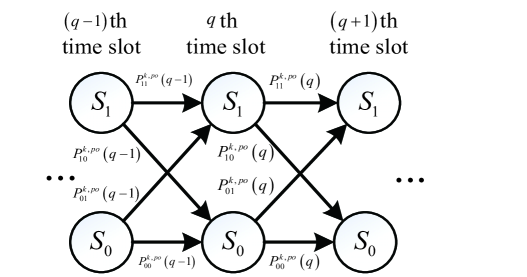
Figure 2: The Markov chain model of power states with a rechargeable energy buffer (${S_{0}}$: Outage, and ${S_{1}}$: Sufficient power).

III-A Power Outage Probability

The power states of ${U_{k}}$ are modeled by a Markov chain, as shown in Fig. 2. In each time slot, ${U_{k}}$ can either be in the power sufficient state ${S_{1}}$ or the power outage state ${S_{0}}$. The states of ${U_{k}}$ at the $\left({q-1}\right)$-th, $q$-th, and $\left({q+1}\right)$-th time slots are illustrated in Fig. 2. The transition probabilities between two power states are represented by $P_{uv}^{k,po}$, where $u,v\in\left\{{0,1}\right\}$ with $0$ corresponding to state ${S_{0}}$ and $1$ corresponding to state ${S_{1}}$. Specifically, the transition probabilities from a given state at $q$-th time slot to the states at $\left({q+1}\right)$-th time slot are expressed as $P_{00}^{k,po}\left(q\right)$, $P_{01}^{k,po}\left(q\right)$, $P_{10}^{k,po}\left(q\right)$, and $P_{11}^{k,po}\left(q\right)$[45]. It is assumed that there are $Q$ continuous time slots, and $C$ denotes the initial state of the battery. To obtain the power outage probability over $Q$ time slots, we calculate the power sufficient probability over $Q$ time slots. First, we calculate the transmission probability $P_{11}^{k,po}\left(q\right)$ at each time slot $q$ $\left({q=1,2,\ldots Q}\right)$ to ensure that the power is sufficient at each time slot $q$ (i.e., the cumulative harvested energy of the energy buffer should not be less than the consumption). Hence, $P_{11}^{k,po}\left(q\right)$ is calculated as

$$P_{11}^{k,po}\left(q\right) =\Pr\left({\sum\limits_{l=1}^{q}{{E_{k}}}+C\geq q{E_{s}}}\right)$$

$$=\Pr\left({\sum\limits_{l=1}^{q}{\eta\left({1-\theta}\right){\beta_{k}}\frac{{{P_{\text{AP}}}}}{L}{T_{s}}{\cal Z}_{l}^{2}}+C\geq q{E_{s}}}\right)$$

$$=\Pr\left({\sum\limits_{l=1}^{q}{{\cal Z}_{l}^{2}}\geq\frac{{L\left({q{E_{s}}-C}\right)}}{{\eta\left({1-\theta}\right){\beta_{k}}{P_{\text{AP}}}{T_{s}}}}}\right),$$ (16)

where $\mathcal{Z}_{l}={\sum\limits_{\ell=1}^{L}{\left({h_{k,\ell}^{0}+\sum\limits_{i=1}^{N}{{h_{\ell,i}}{g_{k,i}}}}\right)}}$.

We first derive the probability density function (PDF) of ${\sum\limits_{l=1}^{q}{{\mathcal{Z}_{l}^{2}}}}$. Let ${{\mathcal{V}_{\ell i}}}={{h_{\ell,i}}{g_{k,i}}}$, the $n$-th moment of ${{\mathcal{V}_{\ell i}}}$ can be expressed as

$${\mu_{{{\mathcal{V}_{\ell i}}}}}\left(n\right)=\lambda_{\ell i}^{-n}\frac{{\Gamma\left({{m_{\ell,i}}+n/2}\right)\Gamma\left({{m_{k,i}}+n/2}\right)}}{{\Gamma\left({{m_{\ell,i}}}\right)\Gamma\left({{m_{k,i}}}\right)}},$$ (17)

where ${\lambda_{\ell i}}=\sqrt{\frac{{{m_{\ell,i}}}}{{{\Omega_{\ell,i}}}}\frac{{{m_{k,i}}}}{{{\Omega_{k,i}}}}}$. The detailed dervation of (17) is given in Appendix A.

Let ${G_{\ell}}=\sum\nolimits_{i=1}^{N}{{\mathcal{V}_{\ell i}}}$. Using multinomial expansion [47], the $n$-th moment of ${G_{\ell}}$, i.e., ${\mu_{{G_{\ell}}}}\left(n\right)\buildrel\Delta\over{=}{\rm{E}}\left({G_{\ell}^{n}}\right)$, can be obtained as

$${\mu_{{G_{\ell}}}}\left(n\right) =\sum\limits_{{n_{1}}=0}^{n}{\sum\limits_{{n_{2}}=0}^{{n_{1}}}{\cdots\sum\limits_{{n_{N-1}}=0}^{{n_{N-2}}}{\left({\begin{array}[]{*{20}{c}}n\\ {{n_{1}}}\end{array}}\right)}}}\left({\begin{array}[]{*{20}{c}}{{n_{1}}}\\ {{n_{2}}}\end{array}}\right)\cdots\left({\begin{array}[]{*{20}{c}}{{n_{N-2}}}\\ {{n_{N-1}}}\end{array}}\right)$$ (24)

$$\times{\mu_{{\mathcal{V}_{\ell i}}}}\left({n-{n_{1}}}\right){\mu_{{\mathcal{V}_{\ell i}}}}\left({{n_{1}}-{n_{2}}}\right)\cdots{\mu_{{\mathcal{V}_{\ell i}}}}\left({{n_{N-1}}}\right).$$ (25)

From (17) and (24), the first and second moments of ${G_{\ell}}$ is obtained as

$${\mu_{{G_{\ell}}}}\left(1\right)=\sum\limits_{i=1}^{N}{{\mu_{{{\cal V}_{\ell i}}}}\left(1\right)},$$ (26)

$${\mu_{{G_{\ell}}}}\left(2\right)=\sum\limits_{i=1}^{N}{{\mu_{{{\cal V}_{\ell i}}}}\left(2\right)}+2\sum\limits_{i=1}^{N}{{\mu_{{{\cal V}_{\ell i}}}}\left(1\right)}\sum\limits_{i^{\prime}=i+1}^{N}{{\mu_{{{\cal V}_{\ell i^{\prime}}}}}\left(1\right)}.$$ (27)

Since $h_{k,\ell}^{0}\sim{\rm{Nakagami}}\left({m_{k,\ell}^{0},\Omega_{k,\ell}^{0}}\right)$, one has

$${\mu_{h_{k,\ell}^{0}}}\left(n\right)=\frac{{\Gamma\left({m_{k,\ell}^{0}+n/2}\right)}}{{\Gamma\left({m_{k,\ell}^{0}}\right)}}{\left({\frac{{m_{k,\ell}^{0}}}{{\Omega_{k,\ell}^{0}}}}\right)^{-n/2}}.$$ (28)

Let ${\cal P_{\ell}}=h_{k,\ell}^{0}+{G_{\ell}}$. The $n$-th moment of $\mathcal{P_{\ell}}$ can be expressed as ${\mu_{\mathcal{P_{\ell}}}}\left(n\right)\buildrel\Delta\over{=}{\rm{E}}\left(P_{\ell}^{n}\right)={\rm{E}}\left({{{\left(h_{k,\ell}^{0}+{G_{\ell}}\right)}^{n}}}\right)$, where ${h_{k,\ell}^{0}}$ and ${G_{\ell}}$ are mutually independent. Using the binomial theorem, ${\mu_{\mathcal{P_{\ell}}}}\left(n\right)$ is calculated as

$${\mu_{\cal P_{\ell}}}\left(n\right) ={\rm{E}}\left[{\sum\limits_{\varepsilon=0}^{n}{\left({\begin{array}[]{*{20}{c}}n\\ \varepsilon\end{array}}\right)h_{k,\ell}^{0,\varepsilon}G_{\ell}^{n-\varepsilon}}}\right]$$ (31)

$$=\sum\limits_{\varepsilon=0}^{n}{\left({\begin{array}[]{*{20}{c}}n\\ \varepsilon\end{array}}\right){\mu_{h_{k,\ell}^{0}}}\left(\varepsilon\right){\mu_{{G_{\ell}}}}\left({n-\varepsilon}\right)}.$$ (34)

Hence, one has

$${\mu_{\mathcal{P_{\ell}}}}\left(1\right)={\mu_{h_{k,\ell}^{0}}}\left(1\right)+{\mu_{G_{\ell}}}\left(1\right),$$ (35)

$${\mu_{\mathcal{P_{\ell}}}}\left(2\right)={\mu_{h_{k,\ell}^{0}}}\left(2\right)+{\mu_{G_{\ell}}}\left(2\right)+2{\mu_{{h_{k,\ell}^{0}}}}\left(1\right){\mu_{G_{\ell}}}\left(1\right).$$ (36)

The distribution of $\mathcal{P_{\ell}}$ can be approximated with a Gamma distribution by the moment-matching approach [48, 49], i.e.,

$${\mathcal{P_{\ell}}}\sim\text{Gamma}\left({\chi,\phi}\right),$$ (37)

where

$$\chi=\frac{{{{\left[{{\rm{E}}\left({\cal P_{\ell}}\right)}\right]}^{2}}}}{{{\rm{Var}}\left({\cal P_{\ell}}\right)}}=\frac{{{{\left[{{\mu_{\cal P_{\ell}}}\left(1\right)}\right]}^{2}}}}{{{\mu_{\cal P_{\ell}}}\left(2\right)-{{\left[{{\mu_{\cal P_{\ell}}}\left(1\right)}\right]}^{2}}}},$$ (38)

$$\phi=\frac{{{\rm{E}}\left({\cal P_{\ell}}\right)}}{{{\rm{Var}}\left({\cal P_{\ell}}\right)}}=\frac{{{\mu_{\cal P_{\ell}}}\left(1\right)}}{{{\mu_{\cal P_{\ell}}}\left(2\right)-{{\left[{{\mu_{\cal P_{\ell}}}\left(1\right)}\right]}^{2}}}}.$$ (39)

Since ${\cal Z}_{l}=\sum\limits_{\ell=1}^{L}{{{\cal P}_{\ell}}}$, one has ${\mathcal{Z}_{l}}\sim\text{Gamma}\left({L\chi,\phi}\right)$. The mean and variance of ${\cal Z}_{l}$ are ${\rm{E}}\left({\cal Z}_{l}\right)=L\chi/\phi$ and ${\rm{Var}}\left({\cal Z}_{l}\right)=L\chi/{\phi^{2}}$, respectively.

Let $\sum\limits_{l=1}^{q}{{\cal Z}_{l}^{2}}=\mathcal{T}$. $\mathcal{T}$ follows the non-central Chi-square distribution with $q$ degrees of freedom. Therefore, the PDF of $\mathcal{T}$ is expressed as

$$f_{\mathcal{T}}\left(x\right)=\frac{1}{{2{\sigma^{2}}}}{\left({\frac{x}{{{s^{2}}}}}\right)^{\frac{{q-2}}{4}}}{e^{-\frac{{{s^{2}}+x}}{{2{\sigma^{2}}}}}}{I_{\frac{q}{2}-1}}\left({\frac{s}{{{\sigma^{2}}}}\sqrt{x}}\right),$$ (40)

where ${\sigma^{2}}={\rm{Var}}\left(\mathcal{Z}_{l}\right)$ and ${s}=\sqrt{q{{\left({{\rm{E}}\left(\mathcal{Z}_{l}\right)}\right)}^{2}}}$. Thus, ${P^{k,po}_{11}}\left(q\right)$ can be calculated as

$${P^{k,po}_{11}}\left(q\right)=\int_{\frac{{L\left({q{E_{s}}-C}\right)}}{{\eta\left({1-\theta}\right){\beta_{k}}{P_{\text{AP}}}{T_{s}}}}}^{\infty}{f_{\mathcal{T}}\left(x\right)}dx$$

$$=\sum\limits_{\varsigma=0}^{\infty}\!\!\!{\sum\limits_{p=0}^{{}^{\frac{q}{2}-1+\varsigma}}\!\!\!{\frac{{{s^{2\varsigma}}{e^{-\frac{{{s^{2}}}}{{2{\sigma^{2}}}}}}}}{{{{\left({2{\sigma^{2}}}\right)}^{\varsigma+p}}\varsigma!}}}}{e^{-\frac{{L\left({q{E_{s}}-C}\right)}}{{2{\sigma^{2}}\eta\left({1-\theta}\right){\beta_{k}}{P_{\text{AP}}}{T_{s}}}}}}\frac{{{{\left({\frac{{L\left({q{E_{s}}-C}\right)}}{{\eta\left({1-\theta}\right){\beta_{k}}{P_{\text{AP}}}{T_{s}}}}}\right)}^{p}}}}{{p!}}.$$ (41)

The detailed derivation of (III-A) is given in Appendix B. When ${\beta_{k}}=0$, one has $\mathop{\lim}\limits_{{\beta_{k}}=0}\frac{{L\left({q{E_{s}}-C}\right)}}{{\eta\left({1-\theta}\right){\beta_{k}}{P_{{\rm{AP}}}}{T_{s}}}}=\infty$. Using $\mathop{\lim}\limits_{x\to\infty}{e^{-x}}x=0$, (III-A) can be expressed as $P_{11}^{k,po}\left(q\right)=0$. To ensure $P_{11}^{k,po}\left(q\right)>0$, ${\beta_{k}}$ should be greater than zero.

It is noted that $q\geq 2$ in (III-A) satisfies $\left({\frac{q}{2}-1+\varsigma}\right)\geq 0$. For the special case of $q=1$, one has

$$P_{11}^{k,po}\left({q=1}\right)=\Pr\left({{{\mathcal{Z}_{l}^{2}}}\geq\frac{{L\left({q{E_{s}}-C}\right)}}{{\eta\left({1-\theta}\right){\beta_{k}}{P_{AP}}{T_{s}}}}}\right).$$ (42)

Since ${\mathcal{Z}_{l}}\sim\text{Gamma}\left({L\chi,\phi}\right)$, the cumulative distribution function (CDF) of $\mathcal{Z}_{l}$ can be expressed as

$${F_{{\mathcal{Z}_{l}}}}\left(x\right)=\frac{1}{{\Gamma\left({L\chi}\right)}}\gamma\left({L\chi,\phi x}\right).$$ (43)

For $Y={X^{2}}$, the CDF of $Y$ can be calculated as ${F_{Y}}\left(y\right)={F_{X}}\left({\sqrt{{y}}}\right)$. The CDF of $\mathcal{Z}_{l}^{2}$ is computed as

$${F_{\mathcal{Z}_{l}^{2}}}\left(x\right)=\frac{1}{{\Gamma\left({L\chi}\right)}}\gamma\left({L\chi,\phi{x^{\frac{1}{2}}}}\right).$$ (44)

Thus, (42) can be calculated as

$${P^{k,po}_{11}}\left({q=1}\right)=1-\frac{1}{{\Gamma\left({L\chi}\right)}}\gamma\left({L\chi,\phi{{\left(\frac{{L\left({q{E_{s}}-C}\right)}}{{\eta\left({1-\theta}\right){\beta_{k}}{P_{\text{AP}}}{T_{s}}}}\right)}^{\frac{1}{2}}}}\right).$$ (45)

According to the Markov model presented in Fig. 2, the power outage probability $P^{k,po}$ of ${U_{k}}$ over $Q$ time slots is calculated as

$$P^{k,po}=1-\prod\limits_{q=1}^{Q}{{P^{k,po}_{11}}\left(q\right)}.$$ (46)

Remark 1: For the buffer-less system, ${{P^{k,po}_{11}}\left(q\right)}$ degenerates to ${{P^{k,po}_{11}}\left({q=1}\right)}$ at each time slot. The power sufficient probability of a buffer-less system is $\prod\limits_{q=1}^{Q}{P_{11}^{k,po}\left({1}\right)}$. Hence, the overall power outage $P_{bl}^{k,po}$ of a buffer-less system over $Q$ time slots can be expressed as $P_{bl}^{k,po}=1-{\left({P_{11}^{k,po}\left({1}\right)}\right)^{Q}}$.

Proposition 3.1: The minimum power outage probability can be achieved when the initial state of the battery satisfies the overall power consumption over $Q$ time slots, i.e., $C=Q{E_{s}}$.

Proof: We take the derivative of ${P_{11}^{k,po}\left(q\right)}$. One has

$$\frac{{\partial P_{11}^{k,po}\left(q\right)}}{{\partial C}}=\sum\limits_{\varsigma=0}^{\infty}\frac{{{s^{2\varsigma}}{e^{-\frac{{{s^{2}}}}{{2{\sigma^{2}}}}}}}}{{{{\left({2{\sigma^{2}}}\right)}^{\varsigma}}\varsigma!}}\frac{{{e^{-\frac{{L\left({q{E_{s}}-C}\right)}}{{2{\sigma^{2}}\eta\left({1-\theta}\right){\beta_{k}}{P_{{\rm{AP}}}}{T_{s}}}}}}L}}{{2{\sigma^{2}}\eta\left({1-\theta}\right){\beta_{k}}{P_{{\rm{AP}}}}{T_{s}}}}$$

$$\times\!\left(\!{\sum\limits_{p=0}^{\frac{q}{2}-1+\varsigma}{\frac{{{{\left({\frac{{L\left({q{E_{s}}-C}\right)}}{{\eta\left({1-\theta}\right){\beta_{k}}{P_{{\rm{AP}}}}{T_{s}}}}}\right)}^{p}}}}{{p!}}-\sum\limits_{p=1}^{\frac{q}{2}-1+\varsigma}{\frac{{{{\left({\frac{{L\left({q{E_{s}}-C}\right)}}{{\eta\left({1-\theta}\right){\beta_{k}}{P_{{\rm{AP}}}}{T_{s}}}}}\right)}^{p-1}}}}{{\left({p-1}\right)!}}}}}\!\right)$$

$$\!=\!\sum\limits_{\varsigma=0}^{\infty}\frac{{{s^{2\varsigma}}{e^{-\frac{{{s^{2}}}}{{2{\sigma^{2}}}}}}}}{{{{\left({2{\sigma^{2}}}\right)}^{\varsigma}}\varsigma!}}\frac{{{e^{-\frac{{L\left({q{E_{s}}-C}\right)}}{{2{\sigma^{2}}\eta\left({1-\theta}\right){\beta_{k}}{P_{{\rm{AP}}}}{T_{s}}}}}}L}}{{2{\sigma^{2}}\eta\left({1-\theta}\right){\beta_{k}}{P_{{\rm{AP}}}}{T_{s}}}}\frac{{{{\left(\!{\frac{{L\left({q{E_{s}}-C}\right)}}{{\eta\left({1-\theta}\right){\beta_{k}}{P_{{\rm{AP}}}}{T_{s}}}}}\!\right)}^{\frac{q}{2}-1+\varsigma}}}}{{\left({\frac{q}{2}-1+\varsigma}\right)!}}.$$ (47)

By assigning $\frac{{\partial P_{11}^{k,po}\left(q\right)}}{{\partial C}}=0$, one has $C=q{E_{s}}$. Considering $Q$ time slots, we have that if $C=Q{E_{s}}$, the power outage probability is minimized over $Q$ time slots.

Proposition 3.2: The average residual energy after $Q$ time slots is given by ${C_{R}}=\eta\left({1-\theta}\right){\beta_{k}}{P_{{\rm{AP}}}}{T_{s}}{\rm{Q}}\frac{{\chi\left({L\chi+1}\right)}}{{{\phi^{2}}}}+C-Q{E_{s}}$. Only if $\eta\left({1-\theta}\right){\beta_{k}}{P_{{\rm{AP}}}}{T_{s}}\frac{{\chi\left({L\chi+1}\right)}}{{{\phi^{2}}}}\geq{E_{s}}$, a sustainable wireless node is possible. Otherwise, the system will gradually deteriorate to a buffer-less system.

Proof: We perform the expectation operation on the residual energy after $Q$ time slots. One has

$${C_{R}} ={\rm{E}}\left({\sum\limits_{l=1}^{Q}{{E_{k}}}+C-Q{E_{s}}}\right)$$

$$={\rm{E}}\left({\sum\limits_{l=1}^{Q}{\eta\left({1-\theta}\right){\beta_{k}}\frac{{{P_{{\rm{AP}}}}}}{L}{T_{s}}Z_{l}^{2}}+C-Q{E_{s}}}\right)$$

$$=\eta\left({1-\theta}\right){\beta_{k}}\frac{{{P_{{\rm{AP}}}}}}{L}{T_{s}}{\rm{QE}}\left({Z_{l}^{2}}\right)+C-Q{E_{s}}$$

$$=\eta\left({1-\theta}\right){\beta_{k}}{P_{{\rm{AP}}}}{T_{s}}{\rm{Q}}\frac{{\chi\left({L\chi+1}\right)}}{{{\phi^{2}}}}+C-Q{E_{s}}.$$ (48)

III-B Information Outage Probability and Sum Throughput

The primary goal of energy collection is to provide the energy for exchanging information. When only part of the received power is available for information communication, it is crucial to assess the probability of communication outages. According to the principle of NOMA, the user with better channel conditions performs SIC decoding, while the other user decodes its signal directly[49]. In this paper, based on the path loss[49, 50, 51], it is assumed that ${U_{t}}$ experiences better channel conditions, and there is a fixed decoding order $\left({{U_{r}},{U_{t}}}\right)$ at ${U_{t}}$.

According to (II-B1) and the decoding order $\left({{U_{r}},{U_{t}}}\right)$, ${U_{t}}$ first decodes the signal of ${U_{r}}$ before decoding its own signal. The signal to interference plus noise ratio (SINR) at $U_{t}$ is given by

$${\gamma_{s}}=\frac{{\theta{\beta_{t}}{{\left|{\sum\limits_{\ell=1}^{L}{\left({h_{t,\ell}^{0}+\sum\limits_{i=1}^{N}{{h_{\ell,i}}{g_{t,i}}}}\right)}}\right|}^{2}}{\alpha_{r}}{P_{\text{AP}}}}}{{\theta{\beta_{t}}{{\left|{\sum\limits_{\ell=1}^{L}{\left({h_{t,\ell}^{0}+\sum\limits_{i=1}^{N}{{h_{\ell,i}}{g_{t,i}}}}\right)}}\right|}^{2}}{\alpha_{t}}{P_{\text{AP}}}+L{N_{0}}}}.$$ (49)

Then, ${U_{t}}$ performs SIC to remove the interference from the signal of ${U_{r}}$ and decodes its signal. The signal to noise ratio (SNR) at $U_{t}$ can be expressed as

$${\gamma_{t}}=\frac{{\theta{\beta_{t}}{{\left|{\sum\limits_{\ell=1}^{L}{\left({h_{t,\ell}^{0}+\sum\limits_{i=1}^{N}{{h_{\ell,i}}{g_{t,i}}}}\right)}}\right|}^{2}}{\alpha_{t}}{P_{\mathrm{AP}}}}}{{L{N_{0}}}}.$$ (50)

Meanwhile, ${U_{r}}$ treats the signal of ${U_{t}}$ as interference and decodes its own signal directly. The SINR at $U_{r}$ is obtained as

$${\gamma_{r}}=\frac{{\theta{\beta_{r}}{{\left|{\sum\limits_{\ell=1}^{L}{\left({h_{r,\ell}^{0}+\sum\limits_{i=1}^{N}{{h_{\ell,i}}{g_{r,i}}}}\right)}}\right|}^{2}}{\alpha_{r}}{P_{\mathrm{AP}}}}}{{\theta{\beta_{r}}{{\left|{\sum\limits_{\ell=1}^{L}{\left({h_{r,\ell}^{0}+\sum\limits_{i=1}^{N}{{h_{\ell,i}}{g_{r,i}}}}\right)}}\right|}^{2}}{\alpha_{t}}{P_{\mathrm{AP}}}+L{N_{0}}}}.$$ (51)

Similar to the power outage analysis in section III-A, the information transmission states can also be modeled with a Markov chain, as illustrated in Fig. 3. The Markov chain can achieve a steady state, defined as

$$\left\{{\begin{array}[]{*{20}{c}}{{\pi_{0}^{k}}P_{00}^{k,io}+{\pi_{1}^{k}}P_{10}^{k,io}={\pi_{0}^{k}}},\\ {{\pi_{0}^{k}}P_{01}^{k,io}+{\pi_{1}^{k}}P_{11}^{k,io}={\pi_{1}^{k}}},\end{array}}\right.$$ (54)

where ${\pi_{0}^{k}}$ and ${\pi_{1}^{k}}$ are the steady state probabilities for two states ${T_{0}}$ and ${T_{1}}$, ${\pi_{0}^{k}}+{\pi_{1}^{k}}=1$, $P_{00}^{k,io}+P_{01}^{k,io}=1$, and $P_{10}^{k,io}+P_{11}^{k,io}=1$. Thus, one has

$$\left\{{\begin{array}[]{*{20}{c}}{{\pi_{0}^{k}}=\frac{{P_{10}^{k,io}}}{{P_{01}^{k,io}+P_{10}^{k,io}}}},\\ {{\pi_{1}^{k}}=\frac{{P_{01}^{k,io}}}{{P_{01}^{k,io}+P_{10}^{k,io}}}}.\end{array}}\right.$$ (57)

III-B1 Information Outage Probability of ${U_{r}}$

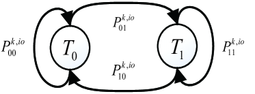
Figure 3: The Markov chain model of information transmission states (${T_{0}}$: Outage, and ${T_{1}}$: Successful transmission).

The transition probability $P_{10}^{r,io}$ denotes the outage probability of ${U_{r}}$, which is calculated as

$$P_{10}^{r,io}=\Pr\left({{\gamma_{r}}<{\gamma_{th}}}\right)$$

$$=\Pr\left({\frac{{\theta{\beta_{r}}{{\left|{\sum\limits_{\ell=1}^{L}{\left({h_{r,\ell}^{0}+\sum\limits_{i=1}^{N}{{h_{\ell,i}}{g_{r,i}}}}\right)}}\right|}^{2}}{\alpha_{r}}{P_{\mathrm{AP}}}}}{{\theta{\beta_{r}}{{\left|{\sum\limits_{\ell=1}^{L}{\left({h_{r,\ell}^{0}+\sum\limits_{i=1}^{N}{{h_{\ell,i}}{g_{r,i}}}}\right)}}\right|}^{2}}{\alpha_{t}}{P_{\mathrm{AP}}}+L{N_{0}}}}<{\gamma_{th}}}\right)$$

$$=\Pr\left({{\mathcal{Z}_{l}^{2}}<\frac{{L{N_{0}}{\gamma_{th}}}}{{\theta{\beta_{r}}{P_{\mathrm{AP}}}\left({{\alpha_{r}}-{\alpha_{t}}{\gamma_{th}}}\right)}}}\right)$$

$$=\frac{1}{{\Gamma\left(L\chi\right)}}\gamma\left({L\chi,\phi{{\left({\frac{{L{N_{0}}{\gamma_{th}}}}{{\theta{\beta_{r}}{P_{\mathrm{AP}}}\left({{\alpha_{r}}-{\alpha_{t}}{\gamma_{th}}}\right)}}}\right)}^{\frac{1}{2}}}}\right),$$ (58)

where ${\gamma_{th}}={2^{R}}-1$ and $R$ is the target rate. $P_{01}^{r,io}=\Pr\left({{\gamma_{r}}\geq{\gamma_{th}}}\right)=1-P_{10}^{r,io}$. Hence, the steady-state probability $\pi_{1}^{r}=P_{01}^{r,io}=1-P_{10}^{r,io}$. After $Q$ time slots, the overall information outage probability of ${U_{r}}$ can be calculated as

$${P^{r,io}}=1-\prod\limits_{q=1}^{Q}{\pi_{1}^{r}}=1-{\left({\pi_{1}^{r}}\right)^{Q}}$$

$$=1-{\left({1-\frac{1}{{\Gamma\left(L\chi\right)}}\gamma\left({L\chi,\phi{{\left({\frac{{L{N_{0}}{\gamma_{th}}}}{{\theta{\beta_{r}}{P_{\mathrm{AP}}}\left({{\alpha_{r}}-{\alpha_{t}}{\gamma_{th}}}\right)}}}\right)}^{\frac{1}{2}}}}\right)}\right)^{Q}}.$$ (59)

III-B2 Information Outage Probability of ${U_{t}}$

Similarly, the $P_{10}^{t,io}$ of ${U_{t}}$ can be expressed as

$$P_{10}^{t,io} =1-\Pr\left({{\gamma_{s}}>{\gamma_{th}},{\gamma_{t}}>{\gamma_{th}}}\right)$$

$$=1-\Pr\left(\!\!\!\begin{array}[]{l}\frac{{\theta{\beta_{t}}{{\left|{\sum\limits_{\ell=1}^{L}{\left({h_{t,\ell}^{0}+\sum\limits_{i=1}^{N}{{h_{\ell,i}}{g_{t,i}}}}\right)}}\right|}^{2}}{\alpha_{r}}{P_{\mathrm{AP}}}}}{{\theta{\beta_{t}}{{\left|{\sum\limits_{\ell=1}^{L}{\left({h_{t,\ell}^{0}+\sum\limits_{i=1}^{N}{{h_{\ell,i}}{g_{t,i}}}}\right)}}\right|}^{2}}{\alpha_{t}}{P_{\mathrm{AP}}}+L{N_{0}}}}>{\gamma_{th}},\\ \frac{{\theta{\beta_{t}}{{\left|{\sum\limits_{\ell=1}^{L}{\left({h_{t,\ell}^{0}+\sum\limits_{i=1}^{N}{{h_{\ell,i}}{g_{t,i}}}}\right)}}\right|}^{2}}{\alpha_{t}}{P_{\mathrm{AP}}}}}{{L{N_{0}}}}>{\gamma_{th}}\end{array}\!\!\!\!\right)$$ (62)

$$=1-\Pr\left({\begin{array}[]{*{20}{l}}{{\mathcal{Z}_{l}^{2}}>\frac{{{\gamma_{th}}L{N_{0}}}}{{\theta{\beta_{t}}{P_{\mathrm{AP}}}\left({{\alpha_{r}}-{\alpha_{t}}{\gamma_{th}}}\right)}},}\\ {{\mathcal{Z}_{l}^{2}}>\frac{{{\gamma_{th}}L{N_{0}}}}{{\theta{\beta_{t}}{\alpha_{t}}{P_{\mathrm{AP}}}}}}\end{array}}\right)$$ (65)

$$=\frac{1}{{\Gamma\left(L\chi\right)}}\gamma\left({L\chi,\phi{{\left({{{\hat{\gamma}}_{t}}}\right)}^{\frac{1}{2}}}}\right),$$ (66)

where ${{\hat{\gamma}}_{t}}=\max\left({\frac{{{\gamma_{th}}L{N_{0}}}}{{\theta{\beta_{t}}{P_{\mathrm{AP}}}\left({{\alpha_{r}}-{\alpha_{t}}{\gamma_{th}}}\right)}},\frac{{{\gamma_{th}}L{N_{0}}}}{{\theta{\beta_{t}}{\alpha_{t}}{P_{\mathrm{AP}}}}}}\right)$. The steady-state probability $\pi_{1}^{t}=1-P_{10}^{t,io}$. After $Q$ time slots, the overall information outage probability of ${U_{t}}$ can be calculated as

$${P^{t,io}}=1-\prod\limits_{q=1}^{Q}{\pi_{1}^{t}}=1-{\left({\pi_{1}^{t}}\right)^{Q}}$$

$$=1-{\left({1-\frac{1}{{\Gamma\left(L\chi\right)}}\gamma\left({L\chi,\phi{{\left({{{\hat{\gamma}}_{t}}}\right)}^{\frac{1}{2}}}}\right)}\right)^{Q}}.$$ (67)

When ${\beta_{k}}=0$, one has $\gamma\left({L\chi,\infty}\right)$ in both (III-B1) and (III-B2). Since $\gamma\left({m,x}\right)=\left({m-1}\right)!\left({1-{e^{-x}}\sum\limits_{n=0}^{m-1}{\frac{{{x^{n}}}}{{n!}}}}\right)$, using $\mathop{\lim}\limits_{x\to\infty}{e^{-x}}x=0$, $\gamma\left({L\chi,\infty}\right)=\left({L\chi-1}\right)!$. Hence $P_{10}^{r,io}=1$ and $P_{10}^{t,io}=1$. To prevent the user from complete information outage, ${\beta_{k}}$ should be greater than zero.

The sum throughput of the proposed system can be expressed as

$$\Psi=R{T_{s}}\left({1-{P^{r,io}}}\right)+R{T_{s}}\left({1-{P^{t,io}}}\right).$$ (68)

III-C Joint Outage Probability

To combine the information outage probability and power outage probability, the joint outage probability can be obtained. For ${U_{k}}$, the joint outage probability is expressed as

$$P_{\text{out}}^{k}=1-\left({1-{P^{k,po}}}\right)\left({1-{P^{k,io}}}\right).$$ (69)

IV Resource Allocation

In this section, we propose a low-complexity power allocation scheme for solving the sum throughput maximization problem with a joint outage probability constraint.

IV-A Problem Formulation

Our goal is to maximize the sum throughput of all users in the proposed system via jointly optimizing the energy-splitting ratios of the STAR-RIS and the power-splitting factor, subject to the joint outage probability requirement of ${U_{r}}$ and ${U_{t}}$. From (68) and (69), the energy-splitting ratios are ${\beta_{r}}$ and ${\beta_{t}}$, and the power-splitting factor is $\theta$. The sum throughput optimization problem can be formulated as

$${{\cal P}_{1}}:\left\{{{\beta_{r}^{*},\beta_{t}^{*},\theta^{*}}}\right\}=\arg\mathop{\max}\limits_{{\beta_{r}},{\beta_{t}},\theta}\Psi\left({{\beta_{r}},{\beta_{t}},\theta}\right)$$ (70)

$$s.t.\ \ C1:0<{\beta_{r}},{\beta_{t}}<1,$$ (70a)

$$\ \ \ \ \ \ C2:{\beta_{r}}+{\beta_{t}}=1,$$ (70b)

$$\ \ \ \ \ \ C3:0<\theta<1,$$ (70c)

$$\ \ \ \ \ \ C4:P_{\text{out}}^{r}<P_{\text{out}}^{r,th},$$ (70d)

$$\ \ \ \ \ \ C5:P_{\text{out}}^{t}<P_{\text{out}}^{t,th}.$$ (70e)

Constraint (70a) ensures that the amplitude coefficients of transmission and reflection for the STAR-RIS are between $0$ and $1$. Constraint (70b) is given to meet the law of energy conservation. Constraint (70c) specifies the range of $\theta$. Constraint (70d) and constraint (70e) guarantee that the joint outage probabilities at ${U_{r}}$ and ${U_{t}}$ are less than the preset threshold $P_{\text{out}}^{r,th}$ and $P_{\text{out}}^{t,th}$, respectively.

IV-B Proposed PSO-PA Algorithm

Since the sum throughput expression in (68) is intractable, we consider a derivative-free optimization method to obtain the optimal solution, which is practical without the computation of gradients[52]. It is difficult to solve the optimization problem using the exhaustive search method in an acceptable time with the increase in network scale. In this context, there are low-complexity optimization algorithms, such as genetic algorithm (GA) and particle swarm optimization (PSO), which have been shown to reach the global optimal solution[53]. Although the GA could work as effectively as PSO, PSO offers a superior computational cost and speed of convergence[54, 53]. Hence, PSO is considered to optimize the energy-splitting ratios ${\beta_{r}}$, ${\beta_{t}}$ and the power-splitting factor $\theta$ for maximizing the sum throughput.

The proposed PSO-PA method first initializes the particles’ positions and velocities. Here, there are three parameters for optimization. The particles’ positions and velocities can be denoted as ${\bf{d}}_{b}^{w}=\left[{d_{b,1}^{w},d_{b,2}^{w},d_{b,3}^{w}}\right]$ and $\mathbf{v}_{b}^{w}=\left[{v_{b,1}^{w},v_{b,2}^{w},v_{b,3}^{w}}\right]$, where $b$ denotes the particle index and $w$ denotes the iteration index. Let ${N_{p}}$ denote the number of particles, and ${N_{i}}$ denote the number of iterations. One has ${{\bf{D}}^{w}}=\left[{{\bf{d}}_{1}^{w},\ldots,{\bf{d}}_{{N_{p}}}^{w}}\right]$. Each particle updates the velocity $v_{b,\zeta}^{w+1}$ based on its current position $d_{b,\zeta}^{w}$, best record ${{\hat{p}}_{b,\zeta}^{w}}$ and global best record ${{\hat{g}}_{\zeta}^{w}}$, where $\zeta\in\left\{{1,2,3}\right\}$. Similarly, one has ${{{\bf{\hat{P}}}}^{w}}=\left[{{\bf{\hat{p}}}_{b}^{w},\ldots,{\bf{\hat{p}}}_{b}^{w}}\right]$ and ${\bf{\hat{G}}}=\left[{{{{\bf{\hat{g}}}}^{1}},\ldots,{{{\bf{\hat{g}}}}^{{N_{i}}}}}\right]$. The iterative equation is expressed as

$$v_{b,\zeta}^{w+1}=\bar{\omega}v_{b,\zeta}^{w}+{C_{1}}{r_{1}}\left({\hat{p}_{b,\zeta}^{w}-d_{b,\zeta}^{w}}\right)+{C_{2}}{r_{2}}\left({\hat{g}_{\zeta}^{w}-d_{b,\zeta}^{w}}\right),$$ (71)

where ${\bar{\omega}}$ is an inertia weight, ${r_{1}}$ and ${r_{2}}$ are chosen independently and uniformly at random to increase the search randomness, and ${C_{1}}$ and ${C_{2}}$ are acceleration instants to control the direction of convergence of the PSO. For example, a larger value of ${C_{1}}$ tends to converge to a personal best solution, leading to a local optimal solution. Correspondingly, a larger value of ${C_{2}}$ tends to converge to the global optimum, where the particles tend to move further distances and increase their exploration of search space. Each particle updates the position based on its current position $d_{b,\zeta}^{w}$, and the velocity $v_{b,\zeta}^{w+1}$, as follows

$$d_{b,\zeta}^{w+1}=d_{b,\zeta}^{w}+v_{b,\zeta}^{w+1}.$$ (72)

Each particle evaluates its penalty fitness function based on its own positions at each iteration. The penalty fitness function is given as follow

$$P_{f}=\Psi\!-\!{\rm{}}\mathchar 22\relax\mkern-10.0mu\lambda\max\left({0,P_{\text{out}}^{r}\!-\!P_{\text{out}}^{r,th}}\right)\!-\!\mathchar 22\relax\mkern-10.0mu\lambda\max\left({0,P_{\text{out}}^{t}\!-\!P_{\text{out}}^{t,th}}\right),$$ (73)

where $\mathchar 22\relax\mkern-10.0mu\lambda$ denotes the penalty factor. The proposed PSO-PA scheme is presented in Algorithm 1.

Algorithm 1 Particle Swarm Optimization Based Power Allocation (PSO-PA)

0:  ${N_{p}}$, ${N_{i}}$, ${C_{1}}$, and ${C_{2}}$.

0:  The optimal ${\beta_{r}^{*},\beta_{t}^{*},\theta^{*}}$.

1:  Randomly initialize the particle positions $\mathbf{d}_{b}^{1}$ and velocities $\mathbf{v}_{b}^{1}$, where $b=1,...,{N_{p}}$.

2:  Set ${\mathbf{\hat{P}^{1}}}=\mathbf{D}^{1}$ and $\mathbf{{\hat{g}^{1}}}=\arg\mathop{\max}\limits_{{\mathbf{{\hat{p}}}_{b}^{1}}\in{{{\bf{\hat{P}}}}^{\bf{1}}}}{P_{f}}$.

3:  for  $w=1:{N_{i}}$ do

4:     for $b=1:{N_{p}}$ do

5:        Calculate particle velocities $\mathbf{v}_{b}^{w+1}$ via (71).

6:        Update particle positions $\mathbf{d}_{b}^{w+1}$ via (72).

7:        if ${P_{f}}\left({\mathbf{d}_{b}^{w+1}}\right)>{P_{f}}\left({\mathbf{{\hat{p}}}_{b}^{w}}\right)$

8:        then $\mathbf{{\hat{p}}}_{b}^{w+1}=\mathbf{d}_{b}^{w+1}$.

9:        else $\mathbf{{\hat{p}}}_{b}^{w+1}=\mathbf{{\hat{p}}}_{b}^{w}$.

10:        end if

11:     end for

12:     Set $\mathbf{{\hat{g}}}^{w+1}=\arg\mathop{\max}\limits_{\mathbf{{\hat{p}}}_{b}^{w+1}\in{\bf{{\hat{P}}}}^{w+1}}{P_{f}}$.

13:  end for

14:  ${\left({\mathbf{{\hat{g}}}^{w}}\right)^{*}}=\arg\mathop{\max}\limits_{\mathbf{{\hat{g}}}^{w}\in{\bf{{\hat{G}}}}}{P_{f}}$.

The time complexity of PSO-PA can be calculated as follows. In PSO-PA, given the ${N_{p}}$ and ${N_{i}}$, the time complexity for initializing the particles’ positions and velocities can be expressed as $O\left({N_{p}}\right)$. The time complexity for searching for the global best record is given by $O\left({{N_{i}}\times{N_{p}}}\right)$. Hence, the overall time complexity is approximated as $O\left({{N_{i}}\times{N_{p}}}\right)+O\left({N_{p}}\right)\approx O\left({{N_{i}}\times{N_{p}}}\right)$.

V Results and Discussion

In this section, power outage probability, information outage probability, sum throughput, and joint outage probability of the proposed system over Nakagami-$m$ fading channels are evaluated. To this end, we set ${P_{{\rm{AP}}}}=1$ Watt (W), ${T_{s}}=1/\left({256{\rm{Kbit/s}}}\right)$, $C=1~{}\rm{\mu J}$, $\tau=-2$ dB, $L=2$, $\eta=0.9$, $Q=5$, and $\vartheta=2$. We consider a two-dimensional Cartesian coordinate location setup as follow. The AP is located at the origin $\left({0,0}\right)$, and the STAR-RIS is located at $\left({16,0}\right)$. The location of $U_{t}$ is $\left({16,2}\right)$, and that of $U_{r}$ is $\left({16,-3}\right)$. For the Nakagami-$m$ fading channel parameters, it is assumed ${m_{0,k}}={m_{i,\ell}}={m_{k,i}}=2$. To verify the effectiveness of the proposed system, the following benchmarks are considered for comparison: i) conventional RIS case. More specifically, we deploy the transmitting-only RIS and the reflecting-only RIS at the same location as the STAR-RIS for full-space coverage, where each reflecting/transmitting-only RIS is equipped with $\frac{N}{2}$ elements for fairness comparison[26]; ii) TDMA case. More specifically, the STAR-RIS adopts the time-switching protocol; iii) buffer-less case. Hence, baseline schemes include the STAR-RIS aided MISO SWIPT-NOMA buffer-less system (referred to as STAR-RIS-BL-NOMA), the RIS and energy buffer aided MISO SWIPT-NOMA system (referred to as RIS-EB-NOMA), and the STAR-RIS and energy buffer aided MISO SWIPT-TDMA system (referred to as STAR-RIS-EB-TDMA). It is noted that the proposed system and STAR-RIS-BL-NOMA have the same information transmission scheme, i.e., STAR-RIS aided NOMA. Hence, we only consider the proposed system, RIS-EB-NOMA, and the STAR-RIS-EB-TDMA when comparing the performance of the information outage probability and sum throughput.

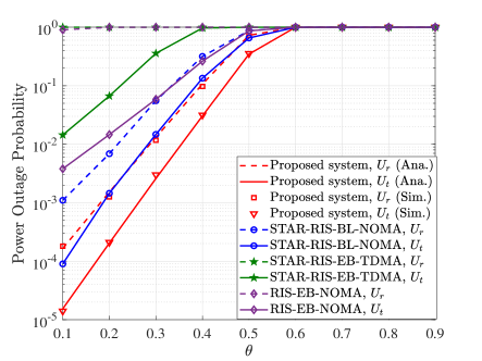
Figure 4: Power outage probability versus power splitting factor $\theta$ of various systems, where $N=18$, ${\beta_{r}}=0.65$, and ${\beta_{t}}=0.35$.

Fig. 4 shows the power outage probability versus power-splitting factor $\theta$ of various systems, where $N=18$, ${\beta_{r}}=0.65$, and ${\beta_{t}}=0.35$. It can be observed that the simulated curves well match with the theoretical ones, which verifies the correctness of the proposed analytical method. Moreover, it is observed that larger values of $\theta$ lead to higher power outage probabilities due to less power being allocated to energy collection. Furthermore, it is seen that the proposed system provides improved power outage probability performance compared to the STAR-RIS-BL-NOMA, RIS-EB-NOMA, and STAR-RIS-EB-TDMA. For example, when $\theta=0.3$, the power outage probability of the proposed system at ${U_{r}}$ is approximately $80\%$ lower than that of the STAR-RIS-BL-NOMA. It is also seen that the proposed system yields an improved performance compared to the RIS-EB-NOMA. This is because the STAR-RIS can be configured for a full-space electromagnetic propagation environments, whereas the conventional RIS requires both the transmitting-only RIS and the reflecting-only RIS to provide full-space coverage. It is shown that the proposed system outperforms the STAR-RIS-EB-TDMA. The reason is that ${U_{r}}$ and ${U_{t}}$ can utilize the same block of time-frequency resources in NOMA, thus achieving a multiplexing gain compared with the TDMA.

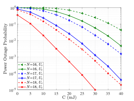
Figure 5: Power outage probability versus the initial energy $C$ for the proposed system with various values of $N$, where ${\beta_{r}}=0.65$, ${\beta_{t}}=0.35$, and $\theta=0.5$.

Fig. 5 illustrates the power outage probability versus the initial energy $C$ for the proposed system with various values of $N$, where ${\beta_{r}}=0.65$, ${\beta_{t}}=0.35$, and $\theta=0.5$. It is observed that the increase in the number of STAR-RIS elements significantly improves the power outage probability performance. For example, when $C=15$ mJ, the outage probability at $U_{r}$ for $N=18$ is approximately $85\%$ lower than that of $N=17$ while the outage probability at $U_{r}$ for $N=17$ is approximately $60\%$ lower than that case where $N=16$. It is also observed that an increase in $C$ yields a better power outage probability performance, especially when $N$ is larger. For example, when $N=18$, an increase in $C$ from $20$ to $25$ reduces the outage probability of $U_{t}$ from ${10^{-3}}$ to ${10^{-4}}$.

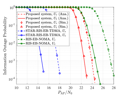
Figure 6: Information outage probability versus the transmit SNR of various systems, where $N=18$, $\theta=0.5$, ${\beta_{r}}=0.6$, ${\beta_{t}}=0.4$, ${\alpha_{r}}=0.6$, ${\alpha_{t}}=0.4$, and $R=1$.

Fig. 6 depicts the information outage probability versus the transmit SNR of various systems, where $N=18$, $\theta=0.5$, ${\beta_{r}}=0.6$, ${\beta_{t}}=0.4$, ${\alpha_{r}}=0.6$, ${\alpha_{t}}=0.4$, and $R=1$. It can be observed that the STAR-RIS-EB-TDMA outperforms the proposed system in terms of the information outage probability. The reason behind this is that there is no inter-user interference with STAR-RIS-EB-TDMA. Moreover, it can be seen that the proposed system outperforms the RIS-EB-NOMA. For example, for a target information outage probability of ${10^{-3}}$, the proposed system shows a gain of $3.5$ dB compared to the RIS-EB-NOMA for $U_{r}$.

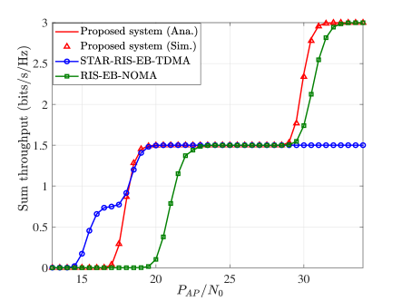
Figure 7: Sum throughput versus transmit SNR of various systems, where $N=18$, $\theta=0.5$, ${\beta_{r}}=0.65$, ${\beta_{t}}=0.35$, ${\alpha_{r}}=0.95$, ${\alpha_{t}}=0.05$, and $R=1.5$.

Fig. 7 shows the sum throughput versus transmit SNR of various systems, where $N=18$, $\theta=0.5$, ${\beta_{r}}=0.65$, ${\beta_{t}}=0.35$, ${\alpha_{r}}=0.95$, ${\alpha_{t}}=0.05$, and $R=1.5$. It is observed that the proposed system can provides a improved sum throughput performance compared with baseline schemes. This is because compared to TDMA, the ${U_{r}}$ and ${U_{t}}$ can utilize the same block of time-frequency resources in NOMA to obtain a multiplexing gain. Moreover, in NOMA, the STAR-RIS adopts the energy-splitting protocol and exploit the proper energy-splitting ratios to obtain an enhanced performance. At low SNR, the performance of the proposed system is slightly worse than that of STAR-RIS-EB-TDMA. The reason behind this is that the poor information outage performance of the proposed system at low SNR affects the sum throughput performance. Moreover, it is observed that an intersection exists between the curves of RIS-EB-NOMA and STAR-RIS-EB-TDMA. The reason lies that the beamforming gain of the STAR-RIS takes the lead and the multiplexing gain is not obvious at low SNR, whereas the multiplexing gain enhances and ultimately surpasses the beamforming gain as a leading factor at high SNR.

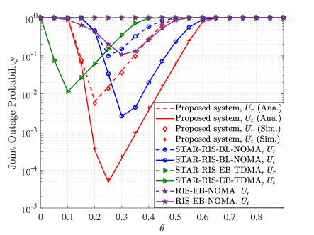
Figure 8: Joint outage probability versus power splitting factor $\theta$ of various systems, where $N=18$, ${P_{{\rm{AP}}}}/{N_{0}}=25$ dB, ${\beta_{r}}=0.6$, ${\beta_{t}}=0.4$, ${\alpha_{r}}=0.7$, and ${\alpha_{t}}=0.3$.

Fig. 8 plots the joint outage probability versus power splitting factor $\theta$ of various systems, where $N=18$, ${P_{{\rm{AP}}}}/{N_{0}}=25$ dB, ${\beta_{r}}=0.6$, ${\beta_{t}}=0.4$, ${\alpha_{r}}=0.7$, and ${\alpha_{t}}=0.3$. It is noticed that an optimal value of $\theta$ exists, which balances the power and information outage probabilities to minimize the joint outage probability. It is observed that the proposed system can obtain better joint outage probability performance compared with the baseline schemes. For example, when $\theta=0.3$, the joint outage probability of the proposed system at $U_{t}$ is ${10^{-3}}$ while that of the STAR-RIS-BL-NOMA is ${10^{-2}}$. It is also noticed that the optimal value of $\theta$ for $U_{t}$ is larger than that for $U_{r}$. This is because $U_{t}$ is a close user, which experiences better channel conditions than $U_{r}$ and can allocate more power for information decoding. Moreover, the STAR-RIS-EB-TDMA slightly outperforms the proposed system for small values of $\theta$. This is because the STAR-RIS-EB-TDMA has a better information outage probability than the proposed system. When $\theta$ is small, the poor information outage probability of the proposed system damages the joint outage probability performance. However, with the increase of $\theta$ and the improvement in the information outage probability performance, the proposed system is superior to the STAR-RIS-EB-TDMA scheme.

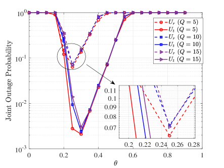
Figure 9: Joint outage probability versus power-splitting factor $\theta$ of the proposed system for various values of $Q$, where $N=17$, ${P_{{\rm{AP}}}}/{N_{0}}=24$ dB, ${\beta_{r}}=0.6$, ${\beta_{t}}=0.4$, ${\alpha_{r}}=0.7$, and ${\alpha_{t}}=0.3$.

Fig. 9 shows the joint outage probability versus power splitting factor $\theta$ of the proposed system for various values of $Q$, where $N=17$, ${P_{{\rm{AP}}}}/{N_{0}}=24$ dB, ${\beta_{r}}=0.6$, ${\beta_{t}}=0.4$, ${\alpha_{r}}=0.7$, and ${\alpha_{t}}=0.3$. It is observed that the joint outage probability performance decreases with the increase of $Q$. This is because as the number of continuous time slots $Q$ increases, both information outage and power outage increase. Moreover, it is observed that as $Q$ increases, the performance degradation becomes smaller. For example, the gap between the curves of $Q=10$ and $Q=15$ is relatively small.

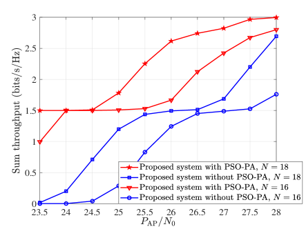
Figure 10: Optimized sum throughput versus transmit SNR of the proposed system with various values of $N$, where ${\alpha_{r}}=0.7$, ${\alpha_{t}}=0.3$, and $R=1.5$.

Fig. 10 plots the optimized sum throughput versus transmit SNR of the proposed system with various values of $N$, where ${\alpha_{r}}=0.7$, ${\alpha_{t}}=0.3$, and $R=1.5$. It is observed that the proposed PSO-PA method can improve the sum throughput performance of the proposed system. For example, for a target sum throughput of $2$ bits/s/Hz, the proposed system with the PSO-PA method and $N=18$ can obtain a $2$ dB gain compared with the proposed system without PSO-PA. As the transmit SNR increases, the PSO-PA method can optimize the sum throughput and balance information transmission and energy harvesting to meet the joint outage probability requirement by adjusting the power-splitting factor and the STAR-RIS’s energy-splitting ratios.

VI Conclusion

In this paper, we have investigated a STAR-RIS and energy buffer aided MISO SWIPT-NOMA system, in which the power transfer and information transmission states are modeled using Markov chains. Moreover, the power outage probability, information outage probability, and sum throughput expressions for the proposed system were derived in closed-form over Nakagami-$m$ fading channels. From the perspective of power and information outage, the joint outage probability was analyzed to investigate the overall network performance. Both theoretical analysis and simulations showed that the proposed system yields an improved performance compared to the selected baseline schemes. Furthermore, the PSO-PA algorithm was designed to maximize the sum throughput with a constraint on the joint outage probability. Results showed that the proposed PSO-PA method significantly improves the sum throughput performance of the proposed system. Thanks to the aforementioned advantages, the proposed system could offer a promising candidate for large-scale, low-power, and sustainable IoT applications.

Appendix A

In this appendix, the $n$-th moment of ${{\mathcal{V}_{\ell i}}}$ is derived. Since ${h_{\ell,i}}\sim{\rm{Nakagami}}\left({{m_{\ell,i}},{\Omega_{\ell,i}}}\right)$ and ${g_{k,i}}\sim{\rm{Nakagami}}\left({{m_{k,i}},{\Omega_{k,i}}}\right)$, the PDFs of ${h_{\ell,i}}$ and ${g_{k,i}}$ are expressed as

$${f_{{h_{\ell,i}}}}\left({x;{m_{\ell,i}},{\Omega_{\ell,i}}}\right)=\frac{{2{m_{\ell,i}}^{{m_{\ell,i}}}}}{{\Gamma\left({{m_{\ell,i}}}\right){\Omega_{\ell,i}}^{{m_{\ell,i}}}}}{x^{{}^{2{m_{\ell,i}}-1}}}{e^{-\frac{{{m_{\ell,i}}}}{{{\Omega_{\ell,i}}}}{x^{2}}}},$$ (74)

$${f_{{g_{k,i}}}}\left({x;{m_{k,i}},{\Omega_{k,i}}}\right)=\frac{{2{m_{k,i}}^{{m_{k,i}}}}}{{\Gamma\left({{m_{k,i}}}\right){\Omega_{k,i}}^{{m_{k,i}}}}}{x^{{}^{2{m_{k,i}}-1}}}{e^{-\frac{{{m_{k,i}}}}{{{\Omega_{k,i}}}}{x^{2}}}}.$$ (75)

Let $Z=XY$, ${f_{Z}}\left(z\right)=\int\limits_{0}^{\infty}{\frac{1}{x}{f_{Y}}\left({\frac{z}{x}}\right)}{f_{X}}\left(x\right)dx$. Since ${{\mathcal{V}_{\ell i}}}={{h_{\ell,i}}{g_{k,i}}}$, the PDF of ${{\mathcal{V}_{\ell i}}}$ is expressed as

$${f_{{{\mathcal{V}_{\ell i}}}}}\left(z\right) =\frac{{4{m_{\ell,i}}^{{m_{\ell,i}}}{m_{k,i}}^{{m_{k,i}}}}}{{\Gamma\left({{m_{\ell,i}}}\right){\Omega_{\ell,i}}^{{m_{\ell,i}}}\Gamma\left({{m_{k,i}}}\right){\Omega_{k,i}}^{{m_{k,i}}}}}{z^{2{m_{k,i}}-1}}$$

$$\times\int\limits_{0}^{\infty}{{x^{2{m_{\ell,i}}-2{m_{k,i}}-1}}}{e^{\left({-\frac{{{m_{\ell,i}}}}{{{\Omega_{\ell,i}}}}{x^{2}}-\frac{{{m_{k,i}}}}{{{\Omega_{k,i}}}}{{\left({\frac{z}{x}}\right)}^{2}}}\right)}}dx.$$ (76)

From (​​[55], eq.(3.478.4)), one has

$$\int\limits_{0}^{\infty}{{x^{\bar{v}-1}}}\exp\left({-\bar{\beta}{x^{\bar{p}}}-\bar{\gamma}{x^{-\bar{p}}}}\right)dx=\frac{2}{{\bar{p}}}{\left({\frac{{\bar{\gamma}}}{{\bar{\beta}}}}\right)^{\frac{{\bar{\nu}}}{{2\bar{p}}}}}{K_{\frac{{\bar{\nu}}}{{\bar{p}}}}}\left({2\sqrt{\bar{\beta}\bar{\gamma}}}\right).$$ (77)

From (77), (A) can be obtained as

$${f_{{{\mathcal{V}_{\ell i}}}}}\left(z\right)=\frac{{4{\lambda}^{{m_{\ell,i}}+{m_{k,i}}}}}{{\Gamma\left({{m_{\ell,i}}}\right)\Gamma\left({{m_{k,i}}}\right)}}{z^{{m_{\ell,i}}+{m_{k,i}}-1}}{K_{{m_{\ell,i}}-{m_{k,i}}}}\left({2z{\lambda_{\ell i}}}\right),$$ (78)

where ${\lambda_{\ell i}}=\sqrt{\frac{{{m_{\ell,i}}}}{{{\Omega_{\ell,i}}}}\frac{{{m_{k,i}}}}{{{\Omega_{k,i}}}}}$.

The $n$-th moment of ${{\mathcal{V}_{i\ell}}}$ is defined as ${\mu_{{{\mathcal{V}_{i\ell}}}}}\left(n\right)\buildrel\Delta\over{=}E\left({{\mathcal{V}_{i\ell}^{n}}}\right)=\int\limits_{0}^{\infty}{{z^{n}}}{f_{{{\mathcal{V}_{i\ell}}}}}\left(z\right)dz$. Based on (78) and with some mathematical operations, ${\mu_{{{\mathcal{V}_{\ell i}}}}}\left(n\right)$ can be obtained as

$${\mu_{{{\mathcal{V}_{\ell i}}}}}\left(n\right)=\lambda_{\ell i}^{-n}\frac{{\Gamma\left({{m_{\ell,i}}+n/2}\right)\Gamma\left({{m_{k,i}}+n/2}\right)}}{{\Gamma\left({{m_{\ell,i}}}\right)\Gamma\left({{m_{k,i}}}\right)}}.$$ (79)

Appendix B

Here, (III-A) is derived. The Bessel function of the first kind can be expanded as follow

$${I_{\frac{q}{2}-1}}\left({\frac{s}{{{\sigma^{2}}}}\sqrt{x}}\right)=\sum\limits_{\varsigma=0}^{\infty}{\frac{{{{\left({\frac{s}{{2{\sigma^{2}}}}\sqrt{x}}\right)}^{\frac{q}{2}-1+2\varsigma}}}}{{\varsigma!\Gamma\left({\frac{q}{2}+\varsigma}\right)}}}.$$ (80)

Thus, (III-A) can be expressed as

$${P^{k}_{11}}\left(q\right)=\int_{\frac{{L\left({q{E_{s}}-C}\right)}}{{\eta\left({1-\theta}\right){\beta_{k}}{P_{AP}}{T_{s}}}}}^{\infty}{f_{\mathcal{T}}\left(x\right)}dx$$

$$=\int_{\frac{{L\left({q{E_{s}}-C}\right)}}{{\eta\left({1-\theta}\right){\beta_{k}}{P_{AP}}{T_{s}}}}}^{\infty}{\frac{1}{{2{\sigma^{2}}}}{{\left({\frac{x}{{{s^{2}}}}}\right)}^{\frac{{q-2}}{4}}}{e^{-\frac{{{s^{2}}+x}}{{2{\sigma^{2}}}}}}{I_{\frac{q}{2}-1}}\left({\frac{s}{{{\sigma^{2}}}}\sqrt{x}}\right)}dx$$

$$=\sum\limits_{\varsigma=0}^{\infty}{\frac{{{e^{-\frac{{{s^{2}}}}{{2{\sigma^{2}}}}}}{s^{2\varsigma}}}}{{{{\left({2{\sigma^{2}}}\right)}^{\frac{q}{2}+2\varsigma}}\varsigma!\Gamma\left({\frac{q}{2}+\varsigma}\right)}}\int_{\frac{{L\left({q{E_{s}}-C}\right)}}{{\eta\left({1-\theta}\right){\beta_{k}}{P_{AP}}{T_{s}}}}}^{\infty}\!\!\!\!\!\!{{e^{-\frac{x}{{2{\sigma^{2}}}}}}{x^{\frac{q}{2}-1+\varsigma}}}}dx.$$ (81)

From (3.351.2) in [55], one has

$$\int\limits_{\bar{u}}^{\infty}{{x^{\omega^{\prime}}}{e^{-\bar{\mu}x}}dx={e^{-\bar{u}\bar{\mu}}}}\sum\limits_{\bar{\ell}=0}^{\omega^{\prime}}{\frac{{\omega^{\prime}!}}{{\bar{\ell}!}}}\frac{{{{\bar{u}}^{\bar{\ell}}}}}{{{{\bar{\mu}}^{\omega^{\prime}-\bar{\ell}+1}}}}.$$ (82)

Using (82), (B) can be calculated as

$${P^{k}_{11}}\left(q\right)=\sum\limits_{\varsigma=0}^{\infty}{\frac{{{e^{-\frac{{{s^{2}}}}{{2{\sigma^{2}}}}}}{s^{2\varsigma}}}}{{{{\left({2{\sigma^{2}}}\right)}^{\frac{q}{2}+2\varsigma}}\varsigma!\Gamma\left({\frac{q}{2}+\varsigma}\right)}}}{e^{-\frac{{L\left({q{E_{s}}-C}\right)}}{{2{\sigma^{2}}\eta\left({1-\theta}\right){\beta_{k}}{P_{\rm{AP}}}{T_{s}}}}}}$$

$$\times\sum\limits_{p=0}^{{}^{\frac{q}{2}-1+\varsigma}}{\frac{{\left({\frac{q}{2}-1+\varsigma}\right)!{{\left({\frac{{L\left({q{E_{s}}-C}\right)}}{{\eta\left({1-\theta}\right){\beta_{k}}{P_{\rm{AP}}}{T_{s}}}}}\right)}^{p}}}}{{p!{{\left({\frac{1}{{2{\sigma^{2}}}}}\right)}^{\frac{q}{2}+\varsigma-p}}}}}$$

$$=\sum\limits_{\varsigma=0}^{\infty}{\sum\limits_{p=0}^{{}^{\frac{q}{2}-1+\varsigma}}{\frac{{{s^{2\varsigma}}{e^{-\frac{{{s^{2}}}}{{2{\sigma^{2}}}}}}}}{{{{\left({2{\sigma^{2}}}\right)}^{\varsigma+p}}\varsigma!}}}}{e^{-\frac{{L\left({q{E_{s}}-C}\right)}}{{2{\sigma^{2}}\eta\left({1-\theta}\right){\beta_{k}}{P_{\rm{AP}}}{T_{s}}}}}}\frac{{{{\left({\frac{{L\left({q{E_{s}}-C}\right)}}{{\eta\left({1-\theta}\right){\beta_{k}}{P_{\rm{AP}}}{T_{s}}}}}\right)}^{p}}}}{{p!}}.$$ (83)

References

• [1] T. Malik, K. Malik, A. Afzal, M. Ibrar, L. Wang, H. Song, and N. Shah, “RL-IoT: Reinforcement learning-based routing approach for cognitive radio-enabled IoT communications,” IEEE Internet Things J., vol. 10, no. 2, pp. 1836–1847, Jan. 2023.
• [2] J. Hwang, L. Nkenyereye, N. Sung, J. Kim, and J. Song, “IoT service slicing and task offloading for edge computing,” IEEE Internet Things J., vol. 8, no. 14, pp. 11526–11547, Jul. 2021.
• [3] L. Chai, L. Bai, T. Bai, J. Choi, and W. Zhang, “RIS-aided SCMA-based SWIPT systems: Design and optimization,” IEEE Trans. Veh. Technol., vol. 72, no. 5, pp. 6238–6252, May 2023.
• [4] K. Choi, L. Ginting, A. Aziz, D. Setiawan, J. Park, S. Hwang, D. Kang, M. Chung, and D. Kim, “Toward realization of long-range wireless-powered sensor networks,” IEEE Wireless Commun., vol. 26, no. 4, pp. 184–192, Aug. 2019.
• [5] R. Zhang, K. Xiong, Y. Lu, P. Fan, D. Ng, and K. Letaief, “Energy efficiency maximization in RIS-assisted SWIPT networks with RSMA: A PPO-based approach,” IEEE J. Sel. Areas Commun., vol. 41, no. 5, pp. 1413–1430, May 2023.
• [6] L. Dai, B. Wang, Y. Yuan, S. Han, I. Chih-lin, and Z. Wang, “Non-orthogonal multiple access for $5$G: Solutions, challenges, opportunities, and future research trends,” IEEE Commun. Mag., vol. 53, no. 9, pp. 74–81, Sept. 2015.
• [7] S. Islam, N. Avazov, O. Dobre, and K. Kwak, “Power-domain non-orthogonal multiple access (NOMA) in $5$G systems: Potentials and challenges,” IEEE Commun. Surv. & Tut., vol. 19, no. 2, pp. 721–742, Oct. 2017.
• [8] J. Tang, J. Luo, M. Liu, D. So, E. Alsusa, G. Chen, K. Wong, and J. Chambers, “Energy efficiency optimization for NOMA with SWIPT,” IEEE J. Sel. Topics Signal Process., vol. 13, no. 3, pp. 452–466, Jun. 2019.
• [9] M. Hedayati and Il-Min Kim, “CoMP-NOMA in the SWIPT networks,” IEEE Trans. Wireless Commun., vol. 19, no. 7, pp. 4549–4562, Jul. 2020.
• [10] T. Nguyen, V. Nguyen, D. Costa, and B. An, “Hybrid user pairing for spectral and energy efficiencies in multiuser MISO-NOMA networks with SWIPT,” IEEE Trans. Commun., vol. 68, no. 8, pp. 4874–4890, Aug. 2020.
• [11] L. Dai, B. Wang, M. Peng, and S. Chen, “Hybrid precoding-based millimeter-wave massive MIMO-NOMA with simultaneous wireless information and power transfer,” IEEE J. Sel. Areas Commun., vol. 37, no. 1, pp. 131–141, Jan. 2019.
• [12] X. Lan, Y. Zhang, Q. Chen, and L. Cai, “Energy efficient buffer-aided transmission scheme in wireless powered cooperative NOMA relay network,” IEEE Trans. Commun., vol. 68, no. 3, pp. 1432–1447, Mar. 2020.
• [13] D. Bapatla and S. Prakriya, “Adaptive multiuser cooperative NOMA scheme with energy buffer-aided near-users for high spectral and energy efficiency,” IEEE Internet Things J., vol. 9, no. 17, pp. 16643–16662, Sept. 2022.
• [14] J. Ren, X. Lei, P. Diamantoulakis, F. Zhou, X. Tang, and O. Dobre, “NOMA for wireless-powered communication networks with buffered sources,” IEEE Trans. Veh. Technol., vol. 70, no. 9, pp. 9088–9102, Sept. 2021.
• [15] C. Pan, H. Ren, K. Wang, W. Xu, M. Elkashlan, A. Nallanathan, and L. Hanzo, “Multicell MIMO communications relying on intelligent reflecting surfaces,” IEEE Trans. Wireless Commun., vol. 19, no. 8, pp. 5218–5233, Aug. 2020.
• [16] J. He, H. Wymeersch, and M. Juntti, “Channel estimation for RIS-aided mmWave MIMO systems via atomic norm minimization,” IEEE Trans. Wireless Commun., vol. 20, no. 9, pp. 5786–5797, Sept. 2021.
• [17] A. Ranjha, and G. Kaddoum, “URLLC facilitated by mobile UAV relay and RIS: A joint design of passive beamforming, blocklength, and UAV positioning,” IEEE Internet Things J., vol. 8, no. 6, pp. 4618–4627, Mar. 2021.
• [18] D. Ng and R. Schober, “Secure and green SWIPT in distributed antenna networks with limited backhaul capacity,” IEEE Trans. Wireless Commun., vol. 14, no. 9, pp. 5082–5097, Sept. 2015.
• [19] R. Ma, J. Tang, X. Zhang, K. Wong, and J. Chambers, “Energy efficiency optimization for mutual-coupling-aware wireless communication system based on RIS-enhanced SWIPT,” IEEE Internet Things J., early access, 2023, doi: 10.1109/JIOT.2023.3241168.
• [20] Q. Wu and R. Zhang, “Weighted sum power maximization for intelligent reflecting surface aided SWIPT,” IEEE Wireless Commun. Lett., vol. 9, no. 5, pp. 586–590, May 2020.
• [21] J. Ren, X. Lei, Z. Peng, X. Tang, and O. Dobre, “RIS-assisted cooperative NOMA with SWIPT,” IEEE Wireless Commun. Lett., vol. 12, no. 3, pp. 446–450, Mar. 2023.
• [22] Q. Liu, M. Lu, N. Li, M. Li, F. Li, and Z. Zhang, “Joint beamforming and power splitting optimization for RIS-assited cooperative SWIPT NOMA system,” in Proc. 2022 IEEE Wireless Commun. Netw. Conf., Austin, TX, USA, pp. 351–356, Apr. 2022.
• [23] G. Zhang, X. Gu, W. Duan, M. Wen, J. Choi, F. Gao, and P. Ho, “Hybrid time-switching and power-splitting EH relaying for RIS-NOMA downlink,” IEEE Trans. Cogn. Commun. Netw., vol. 9, no. 1, pp. 146–158, Feb. 2023.
• [24] J. Xu, Y. Liu, X. Mu, and O. Dobre, “STAR-RISs: Simultaneous transmitting and reflecting reconfigurable intelligent surfaces,” IEEE Commun. Lett., vol. 25, no. 9, pp. 3134–3138, Sept. 2021.
• [25] Y. Liu, X. Mu, J. Xu, R. Schober, Y. Hao, H. Poor, and L. Hanzo, “STAR: Simultaneous transmission and reflection for $360^{o}$ coverage by intelligent surfaces,” IEEE Wireless Commun., vol. 28, no. 6, pp. 102–109, Dec. 2021.
• [26] Z. Zhang, J. Chen, Y. Liu, Q. Wu, B. He, and L. Yang, “On the secrecy design of STAR-RIS assisted uplink NOMA networks,” IEEE Trans. Wireless Commun., vol. 21, no. 12, pp. 11207–11221, Dec. 2022.
• [27] X. Mu, Y. Liu, L. Guo, J. Lin, and R. Schober, “Simultaneously transmitting and reflecting (STAR) RIS aided wireless communications,” IEEE Trans. Wireless Commun., vol. 21, no. 5, pp. 3083–3098, May 2022.
• [28] Z. Xie, W. Yi, X. Wu, Y. Liu, and A. Nallanathan, “STAR-RIS aided NOMA in multicell networks: A general analytical framework with Gamma distributed channel modeling,” IEEE Trans. Commun., vol. 70, no. 8, pp. 5629–5644, Aug. 2022.
• [29] Y. Sun, D. Ng, Z. Ding, and R. Schober, “Optimal joint power and subcarrier allocation for full-duplex multicarrier non-orthogonal multiple access systems,” IEEE Trans. Commun., vol. 65, no. 3, pp. 1077–1091, Mar. 2017.
• [30] C. Wu, X. Mu, Y. Liu, X. Gu, and X. Wang, “Resource allocation in STAR-RIS-aided networks: OMA and NOMA,” IEEE Trans. Wireless Commun., vol. 21, no. 9, pp. 7653–7667, Sept. 2022.
• [31] J. Zuo, Y. Liu, Z. Ding, L. Song, and H. Poor, “Joint design for simultaneously transmitting and reflecting (STAR) RIS assisted NOMA systems,” IEEE Trans. Wireless Commun., vol. 22, no. 1, pp. 611–626, Jan. 2023.
• [32] Y. Guo, F. Fang, D. Cai, and Z. Ding, “Energy-efficient design for a NOMA assisted STAR-RIS network with deep reinforcement learning,” IEEE Trans. Veh. Technol., vol. 72, no. 4, pp. 5424–5428, Apr. 2023.
• [33] F. Fang, B. Wu, S. Fu, Z. Ding, and X. Wang, “Energy-efficient design of STAR-RIS aided MIMO-NOMA networks,” IEEE Trans. Commun., vol. 71, no. 1, pp. 498–511, Jan. 2023.
• [34] X. Qin, Z. Song, T. Hou, W. Yu, J. Wang, and X. Sun, “Joint resource allocation and configuration design for STAR-RIS-enhanced wireless-powered MEC,” IEEE Trans. Commun., vol. 71, no. 4, pp. 2381–2395, Apr. 2023.
• [35] W. Du, Z. Chu, G. Chen, P. Xiao, Y. Xiao, X. Wu, and W. Hao, “STAR-RIS assisted wireless powered IoT networks,” IEEE Trans. Veh. Technol., early access, 2023, doi: 10.1109/TVT.2023.3262801.
• [36] K. Xie, G. Cai, G. Kaddoum, and J. He, “Performance analysis and resource allocation of STAR-RIS aided wireless-powered NOMA system,” IEEE Trans. Commun., early access, 2023, doi: 10.1109/TCOMM.2023.3292471.
• [37] P. Zhao, J. Zuo, and C. Wen, “Power allocation and beamforming vectors optimization in STAR-RIS assisted SWIPT,” in Proc. 2022 IEEE Int. Conf. Commun. Technol., Nanjing, China, pp. 1174–1178, Nov. 2022.
• [38] X. Li, Y. Zheng, M. Zeng, Y. Liu, and O. Dobre, “Enhancing secrecy performance for STAR-RIS NOMA networks,” IEEE Trans. Veh. Technol., vol. 72, no. 2, pp. 2684–2688, Feb. 2023.
• [39] P. Tran, B. Nguyen, T. Hoang, X. Le, and V. Nguyen, “Exploiting multiple RISs and direct link for performance enhancement of wireless systems with hardware impairments,” IEEE Trans. Commun., vol. 70, no. 8, pp. 5599–5611, Aug. 2022.
• [40] D. Selimis, K. Peppas, G. Alexandropoulos, and F. Lazarakis, “On the performance analysis of RIS-empowered communications over Nakagami-$m$ fading,” IEEE Commun. Lett., vol. 25, no. 7, pp. 2191–2195, Jul. 2022.
• [41] C. Wu, C. You, Y. Liu, X. Gu, and Y. Cai, “Channel estimation for STAR-RIS-aided wireless communication,” IEEE Commun. Lett., vol. 26, no. 3, pp. 652–656, Mar. 2022.
• [42] Q. Wu and R. Zhang, “Intelligent reflecting surface enhanced wireless network via joint active and passive beamforming,” IEEE Trans. Wireless Commun., vol. 18, no. 11, pp. 5394–5409, Nov. 2019.
• [43] I. Sohn, J. Lee, and S. Lee, “Low-energy adaptive clustering hierarchy using affinity propagation for wireless sensor networks,” IEEE Commun. Lett., vol. 20, no. 3, pp. 558–561, Mar. 2016.
• [44] W. R. Heinzelman, A. Chandrakasan, and H. Balakrishnan, “Energy-efficient communication protocol for wireless microsensor networks,” in Proc. 33rd Annu. Hawaii Int. Conf. Syst. Sci., Maui, HI, USA, pp. 10–21, Jan. 2000.
• [45] Y. Luo, C. Luo, G. Min, G. Parr, and S. McClean, “On the study of sustainability and outage of SWIPT-enabled wireless communications,” IEEE J. Sel. Topics Signal Process., vol. 15, no. 5, pp. 1159–1168, Aug. 2021.
• [46] Y. Chen, S. Lu, H. Kim, D. Blaauw, R. Dreslinski, and T. Mudge, “A low power software-defined-radio baseband processor for the internet of things,” in Proc. IEEE Int. Symp. High Perform. Comput. Architecture, Barcelona, Spain, pp. 40–51, Mar. 2016.
• [47] D. Costa, H. Ding, and J. Ge, “Interference-limited relaying transmissions in dual-hop cooperative networks over Nakagami-$m$ fading,” IEEE Commun. Lett., vol. 15, no. 5, pp. 503–505, May 2011.
• [48] S. Atapattu, R. Fan, P. Dharmawansa, G. Wang, J. Evans, and T. Tsiftsis, “Reconfigurable intelligent surface assisted two-way communications: Performance analysis and optimization,” IEEE Trans. Commun., vol. 68, no. 10, pp. 6552–6567, Oct. 2020.
• [49] T. Wang, M. Badiu, G. Chen, and J. Coon, “Outage probability analysis of STAR-RIS assisted NOMA network with correlated channels,” IEEE Commun. Lett., vol. 26, no. 8, pp. 1774–1778, Aug. 2022.
• [50] C. Zhang, W. Yi, Y. Liu, Z. Ding, and L. Song, “STAR-IOS aided NOMA networks: Channel model approximation and performance analysis,” IEEE Trans. Wireless Commun., vol. 21, no. 9, pp. 6861–6876, Sept. 2022.
• [51] X. Yue, J. Xie, Y. Liu, Z. Han, R. Liu, and Z. Ding, “Simultaneously transmitting and reflecting reconfigurable intelligent surface assisted NOMA networks,” IEEE Trans. Wireless Commun., vol. 22, no. 1, pp. 189–204, Jan. 2023.
• [52] W. Xu, G. Cai, Y. Fang, S. Mumtaz, and G. Chen, “Performance analysis and resource allocation for a relaying LoRa system considering random nodal distances,” IEEE Trans. Commun., vol. 70, no. 3, pp. 1638–1652, Mar. 2022.
• [53] M. Shabanighazikelayeh and E. Koyuncu, “Optimal placement of UAVs for minimum outage probability,” IEEE Trans. Veh. Technol., vol. 71, no. 9, pp. 9558–9570, Sept. 2022.
• [54] S. Shabir and R. Singla, “A comparative study of genetic algorithm and the particle swarm optimization,” Int. J. Electr. Eng, vol. 9, no. 2, pp. 215–223, 2016.
• [55] I. S. Gradshteyn and I. M. Ryzhik, Table of Integrals Series and Products. Amsterdam, The Netherlands: Elsevier, 2007.