The Inflation Attention Threshold and Inflation Surges

Abstract

At the outbreak of the recent inflation surge, the public’s attention to inflation was low but increased rapidly once inflation started to rise. I develop a framework where this behavior is optimal: agents pay little attention to inflation when inflation is low and stable, but they increase their attention once inflation exceeds a certain threshold. Using survey inflation expectations, I estimate the attention threshold to be at an inflation rate of about 4%, with attention in the high-attention regime being twice as high as in the low-attention regime. Embedding this into a general equilibrium monetary model, I find that the inflation attention threshold gives rise to a dynamic non-linearity in the Phillips Curve, rendering inflation more sensitive to fluctuations in the output gap during periods of high attention. When calibrated to match the empirical findings, the model generates inflation and inflation expectation dynamics consistent with the recent inflation surge in the US. The attention threshold induces a state dependency: cost-push shocks become more inflationary in times of loose monetary policy. These state-dependent effects are absent in the model with constant attention or under rational expectations. Following simple Taylor rules triggers frequent and prolonged episodes of heightened attention, thereby increasing the volatility of inflation, and—due to the asymmetry of the attention threshold—also the average level of inflation, which leads to substantial welfare losses.

JEL Codes: E3, E4, E5, E7
Keywords: Inattention, Inflation, Inflation Expectations, Monetary Policy

1 Introduction

Inflation is back. After decades of low and stable inflation, inflation surged in many advanced economies during the recovery phase of the pandemic. Inflation turned out to be higher and more persistent than many expected. With inflation rising, the public’s attention to inflation increased as well (Figure 1). But is this increased attention to inflation merely a byproduct or a driver of high and persistent inflation?

Figure 1: Inflation is back… on people’s minds

Notes: The black-solid line shows the monthly year-on-year US CPI inflation rate, and the blue-dashed line the number of Google searches in the US of inflation (normalized such that the two series have the same maximum).

To shed light on this question, I develop a framework in which agents optimally pay little attention to inflation when inflation is low and stable, but in which attention increases once inflation exceeds a certain threshold. Using household inflation expectations, I estimate the attention threshold to be at an annualized quarter-on-quarter inflation rate of about 4.0%, implying that the US economy in early 2021 entered the high-attention regime, meaning that attention to inflation basically doubled. Introducing this attention framework into an otherwise standard New Keynesian model, I then show that accounting for the attention threshold matters greatly for the model’s predicted inflation dynamics as well as its monetary policy implications. When calibrating the model to match the empirical findings, it generates inflation and inflation expectation dynamics mirroring the ones recently observed in the US. Accounting for varying attention levels also matters for the model’s normative predictions. In particular, I show that following simple Taylor rules can lead to substantially larger welfare losses than absent the attention threshold.

To quantify attention across different attention regimes, I extend the method I proposed in Pfäuti (2023) by allowing for an attention threshold. Attention captures how strongly agents update their inflation expectations in response to forecast errors. I allow for different degrees of attention depending on whether inflation is above or below a certain attention threshold, and I show that one possible explanation for these attention shifts may be that the cost of information decreases, for example, because news media start reporting more prominently about inflation when inflation exceeds the threshold. Consistent with this interpretation, I find that news coverage of inflation is significantly higher in times of higher inflation. In line with my findings, Bracha and Tang (2023) show that higher inflation rates lead to more media reporting about inflation, Larsen et al. (2021) find that news media coverage predicts households’ inflation expectations, and Lamla and Lein (2014) show that more intensive news reporting about inflation improves the accuracy of consumers’ inflation expectations.

I then jointly estimate the attention threshold as well as the attention levels in the two regimes using survey data from the University of Michigan’s Survey of Consumers for the period 1978 to 2023. I estimate an inflation attention threshold of 4.0%, and that attention is about 0.18 when inflation is below the threshold and more than doubles to 0.36 when inflation is above the threshold. An attention level of 0.36 means that following a 1pp forecast error, agents increase their inflation expectations by 0.36pp. Using the Survey of Consumer Expectations from the NY Fed for the period 2013-2023, I obtain similar results: attention in times when inflation was below 4% is about 0.21 and increases to 0.4 when inflation is above 4%. Once I control for the attention threshold, I do not find any evidence that attention increases with inflation within regime.

To understand the implications of these empirical findings for inflation, inflation expectations and monetary policy, I extend the standard New Keynesian model by introducing an attention threshold and changing levels of attention. Firms and households pay limited attention to inflation, as acquiring and processing information about inflation is costly. The main novelty is that I introduce the aforementioned attention threshold: once inflation exceeds this threshold, households and firms pay more attention to inflation.

In a stylized version of the model, I show analytically and graphically how the attention threshold alters the dynamics of inflation. Following a cost-push shock that pushes the economy into the high-attention regime, both the aggregate supply and aggregate demand curve become steeper—thus, the attention threshold gives rise to a dynamic non-linearity in the Phillips Curve and the aggregate demand curve. Additionally, the effects of the ongoing shock are amplified through the heightened attention level, leading to a further upward shift in the AS curve. On top of that, this shift occurs along a steeper AD curve, such that the inflationary effects are even larger. Overall, this stylized example illustrates how an upward shift in attention may lead to self-reinforcing inflation dynamics without large changes in the output gap.

I then calibrate the model to match the estimated attention levels in the two regimes, the attention threshold, and the frequency of staying in the high-attention regime. Accounting for the attention threshold substantially alters the dynamics of inflation and inflation expectations. Following an inflationary supply shock that pushes inflation just above the attention threshold, inflation keeps on increasing through the endogenous attention increase. As attention increases, agents now update their inflation expectations more strongly in response to the increase in inflation. These higher inflation expectations then fuel further inflation increases, leading to higher inflation expectations, and so on. As the shock dies out, inflation starts to decline after some time. However, inflation may remain elevated for a substantial period of time, because once it falls back below the threshold, people pay less attention to inflation, and hence, only slowly revise their inflation expectations downward. As their prior expectations are now relatively high due to the experienced high inflation period, expectations remain persistently high, leading to a slow decline of actual inflation. I show that these patterns of inflation and inflation expectations are consistent with the recent inflation surge in the US: inflation followed a hump-shaped pattern and inflation expectations initially fell short of the actual inflation surge, but then surpassed it once inflation started to decline. The inflation dynamics my model produces are further consistent with the empirical findings in Blanco et al. (2022) who document, for a number of countries and different periods of inflation surges, that (i) inflation stays persistently high after the initial surge and (ii) that short-run inflation expectations initially fall short of actual inflation.

The attention threshold further induces a state dependency. The inflationary effects of cost-push shocks are larger when the shock hits at a time of loose monetary policy, and the total effect is in fact substantially larger than the sum of the two effects in isolation. This state dependency arises due to the heightened attention which—together with loose monetary policy—renders inflation more responsive to cost-push shocks. These state-dependent effects are absent in the economy with a constant level of attention or with full-information rational expectations.

Thus, large shocks—supply or demand—may push the economy into the high-attention regime and therefore, lead to high and persistent inflation rates. However, also relatively small shocks to demand and supply simultaneously can trigger large inflation surges when the combination of the two shocks pushes inflation above the inflation attention threshold. Thus, the model with the attention threshold may predict high-inflation periods at times the model absent the attention threshold or the one under rational expectations would predict a substantially smaller and more transitory increase in inflation.

Thus, accounting for sudden changes in the public’s attention to inflation may help to understand how inflation surges can arise and sustain themselves for a prolonged period, and offers a new perspective on the last two high-inflation episodes in the US. The US economy was in the high-attention regime during the Great Inflation period and recently entered it again in 2021. Reis (2022) shows that inflation expectations have become unanchored in the Great Inflation period, and Hilscher et al. (2022) find that in 2021 the risk of persistently high inflation in the US increased significantly. Both of these findings are consistent with the predictions of my model: in the high-attention regime, inflation expectations are more sensitive to inflation, i.e., they appear to be less anchored, and the regime switch to the high-attention regime increases the risk of persistently high inflation due to the higher sensitivity of inflation expectations.

Taking the attention threshold into account also matters for the model’s normative implications. When monetary policy sets the nominal interest rate following a simple Taylor rule, the associated welfare losses are significantly larger compared to optimal policy rules or a strict inflation targeting rule (similar to the findings in Gáti (2022)). The reason is that under a standard calibration for the Taylor rule, the economy spends a substantial amount of time in the high-attention regime in which inflation is high and volatile. Due to the asymmetry of the attention threshold—attention increases when inflation is particularly high but remains constant when inflation is particularly low—the average level of inflation is higher when the economy is in the high-attention regime frequently. This is in stark contrast to the model without the threshold or the one with fully-informed rational agents, where inflation fluctuates symmetrically around zero. This asymmetry of the attention threshold also offers a potential explanation for why we did not observe long lasting deflationary periods, for example, during the Great financial crisis (Coibion and Gorodnichenko, 2015). In fact, annualized quarter-on-quarter CPI inflation was negative in only 7% of the time between 1978 and 2023, whereas it exceeded the attention threshold of 4.0% about 30% of the time during the same period.

Taylor rules with a high degree of interest-rate smoothing lead to especially large welfare losses in the model with two attention regimes—in contrast to the model under rational expectations in which interest-rate smoothing increases welfare. Interest-rate smoothing introduces additional persistence, such that the periods in the high-attention regime last longer and thus, the average level of inflation as well as its volatility increase. The monetary authority can avoid these large welfare losses by implementing some optimal policy rule: even when monetary policy ignores that private agents pay limited attention to inflation and implements the policy that would be optimal with rational agents, the welfare losses are small and in fact close to the ones in the model with rational agents.

Related literature.

Pfäuti (2023) documents that before the recent inflation surge, attention to inflation was at a historical low. Bracha and Tang (2023) find that when inflation increases, attention to inflation increases as well. Korenok et al. (2022) find, for a large number of countries, that people’s attention to inflation increases with inflation only after inflation exceeds a certain threshold. Using Google search data for the period from 2004 to 2022, they estimate this attention threshold to be at an annualized inflation rate of 3.55% for the US. Cavallo et al. (2017) show that survey respondents in high-inflation environments (Argentina) respond less to information about inflation than in low-inflation environments (United States), which is consistent with higher attention to inflation in high-inflation environments. Weber et al. (2023) confirm, using a range of randomized control trials spanning over several years and different countries, that attention of households and firms is indeed higher in times of high inflation. Kroner (2023) focuses on financial markets and shows that attention—measured as asset price responses to inflation news—is higher in times of high inflation. My key innovation relative to these papers is that I provide estimates of the attention threshold and the attention levels in the two regimes in a way that directly maps into otherwise standard macroeconomic models.

The theoretical insights in this paper contribute to a growing literature on the role of changes in attention and the degree of anchoring of inflation expectations. Evans and Ramey (1995) propose a model in which agents choose how forward-looking they want to be and show that inflation remains stable when agents are not very forward looking. Gáti (2022) studies how changes in the degree of anchoring of long-run inflation expectations affect the optimal monetary policy. In her paper, anchoring changes continuously, thus, can also jump in response to large shocks. In contrast, attention in my model only changes across but not within regime, which is consistent with what I find in the data, namely, that attention is constant within regime. Carvalho et al. (2022) focus on discrete changes in anchoring of long-run inflation expectations, but do so in a partial equilibrium setting. In Pfäuti (2023), I study the implications of low attention for optimal monetary policy when the zero lower bound poses a constraint to monetary policy. In contrast to that paper, I allow here for an inflation attention threshold, whereas Pfäuti (2023) compares economies with different—but time-invariant—degrees of attention. Hazell et al. (2022) show that the greater inflation stability after 1990 is mostly due to more firmly-anchored long-run inflation expectations. Related, Jørgensen and Lansing (2023) find that more strongly anchored inflation expectations can help explain changes in the reduced form Phillips curve, and Afrouzi and Yang (2020) show that in a model of dynamic rational inattention the stance of monetary policy affects the slope of the Phillips curve. The main contribution of the present paper to this literature is that I incorporate and estimate an inflation attention threshold into a general equilibrium model and show how accounting for such a threshold can help us better understand how inflation surges may happen and how they can sustain themselves, as well as the monetary policy implications that follow from such attention-fueled inflation surges.

Outline.

Section 2 explains how I estimate attention and the attention threshold in the data and presents my empirical findings. I introduce the New Keynesian model with limited attention in Section 3, and the model’s positive results in Section 4. In Section 5, I derive the model’s normative implications and Section 6 concludes.

2 Attention and the Inflation Attention Threshold

In this section, I show how I estimate the inflation attention threshold and the different degrees of attention in the two attention regimes, and present the estimation results. To arrive at these results, I extend the method I develop in Pfäuti (2023) by allowing for an inflation-attention threshold. Details on the optimal attention choice are relegated to Appendix A.

Agents hold a subjective model of how inflation evolves. In particular, the agent believes that (demeaned) inflation tomorrow, $\pi^{\prime}$, depends on (demeaned) inflation today, $\pi$, as follows

$$\pi^{\prime}=\rho_{\pi}\pi+\nu,$$

where $\rho_{\pi}\in[0,1]$ denotes the perceived persistence of inflation and $\nu\sim i.i.N.(0,\sigma^{2}_{\nu})$. The agent faces a trade off how attentive she wants to be. On the one hand, making forecast errors is costly, but on the other hand, current inflation is unobservable and acquiring and processing information about it is also costly. I assume that the loss arising from making forecasting mistakes is quadratic with a scaling factor $\chi$ and that the cost of information is linear in mutual information with a scaling factor $\tfrac{1}{\lambda}$.

Assuming a normal prior, the optimal signal the agent acquires then takes the form

$$s=\pi+\varepsilon,$$

with $\varepsilon\sim i.i.N.(0,\sigma^{2}_{\varepsilon})$ (see Matějka and McKay (2015)). Conditional on the signal, and the perceived law of motion, the optimal expectation about inflation tomorrow is given by $\tilde{E}[\pi^{\prime}|s]=\rho_{\pi}E\left[\pi|s\right]$. Bayesian updating implies

$$\tilde{E}[\pi^{\prime}|s]=\rho_{\pi}\left(1-\gamma_{\pi}\right)\widehat{\pi}+\rho_{\pi}\gamma_{\pi}s,$$ (1)

where $\gamma_{\pi}=1-\frac{\sigma^{2}_{\pi|s}}{\sigma^{2}_{\pi}}\in[0,1]$ measures attention to inflation, and $\widehat{\pi}$ denotes the prior mean of $\pi$.

Solving for the optimal level of attention $\gamma_{\pi}$ yields

$$\gamma_{\pi}=max\left\{0,1-\frac{\tfrac{1}{\lambda}}{2\chi\rho_{\pi}^{2}\sigma^{2}_{\pi}}\right\}.$$ (2)

The expression (2) for the optimal attention level shows that when the cost of information $\frac{1}{\lambda}$ is lower, attention is higher.

Dynamics.

To estimate attention in the data, I extend the law of motion of inflation expectations, equation (1), to a dynamic setup. The agent believes that inflation $\pi$ follows

$$\pi_{t}=(1-\rho_{\pi})\underline{\pi}+\rho_{\pi}\pi_{t-1}+\nu_{t},$$

where $\underline{\pi}$ is the agent’s long-run belief about inflation and $\rho_{\pi}$ is the perceived persistence of inflation. I assume that the error term $\nu_{t}$ is normally distributed with mean zero and variance $\sigma^{2}_{\nu}$. The agent receives a signal about inflation of the form

$$s_{t}=\pi_{t}+\varepsilon_{t},$$

where the noise $\varepsilon_{t}$ is assumed to be normally distributed with variance $\sigma^{2}_{\varepsilon}$. Higher attention is reflected in less noise, i.e., a lower $\sigma^{2}_{\varepsilon}$.

Given these assumptions, it follows from the (steady state) Kalman filter that optimal updating is given by

$$\tilde{E}_{t}\pi_{t+1}=(1-\rho_{\pi})\underline{\pi}+\rho_{\pi}\tilde{E}_{t-1}\pi_{t}+\rho_{\pi}\gamma_{\pi}\left(\pi_{t}-\tilde{E}_{t-1}\pi_{t}\right)+u_{t}.$$ (3)

From equation (3), we observe that lower attention, i.e., a lower $\gamma_{\pi}$, implies that the agent updates her expectations to a given forecast error, $(\pi_{t}-\tilde{E}_{t-1}\pi_{t})$, less strongly. Lower attention is reflected in more noisy signals, and more noise means the agent puts less weight on these signals and more weight on the prior.

Attention regimes.

To allow for changes in people’s attention, I assume that attention changes when inflation exceeds a certain threshold $\bar{\pi}$, such that inflation expectations follow the law of motion:

$$\tilde{E}_{t}\pi_{t+1}=\begin{cases}(1-\rho_{\pi})\underline{\pi}+\rho_{\pi}\tilde{E}_{t-1}\pi_{t}+\rho_{\pi}\gamma_{\pi,L}\left(\pi_{t}-\tilde{E}_{t-1}\pi_{t}\right)+u_{t},\text{ when }\pi_{t-1}<\bar{\pi}\\ (1-\rho_{\pi})\underline{\pi}+\rho_{\pi}\tilde{E}_{t-1}\pi_{t}+\rho_{\pi}\gamma_{\pi,H}\left(\pi_{t}-\tilde{E}_{t-1}\pi_{t}\right)+u_{t},\text{ when }\pi_{t-1}>\bar{\pi}.\end{cases}$$ (4)

As shown in the expression for optimal attention (equation (2)), one potential reason for such changes in attention may arise from changes in the cost of information $\frac{1}{\lambda_{r}}$ with $r\in\{L,H\}$. Changes in $\lambda_{r}$ may come from changes in how much the news media report about inflation, with $\lambda_{H}>\lambda_{L}$, assuming that there is more news reporting about inflation in the $H$ regime. I assume that agents do not foresee these changes in news reporting and form their expectations within regime $r$ as if $\lambda_{r}$ would remain unchanged. Hence, when there is more news about inflation in regime $H$, reflected in a lower cost of information $\tfrac{1}{\lambda_{H}}<\tfrac{1}{\lambda_{L}}$, attention is higher: $\gamma_{\pi,H}>\gamma_{\pi,L}$. In the estimation later on, I will test this prediction of the theory rather than impose it, and I will further test whether attention also varies within regime $r$. .

Figure 2 supports the assumption that media reporting about inflation is higher in times of higher inflation. The Figure shows the frequency of the word “inflation” in the New York Times (1970 to July 2023, blue-dashed line) and the Washington Post (1977-2019, red-dashed-dotted line), together with annual CPI inflation (black-solid line). There is a very strong positive correlation between inflation and news coverage of inflation (the correlation between CPI inflation and the two news-coverage series is 0.86 for the New York Times and 0.90 for the Washington Post).

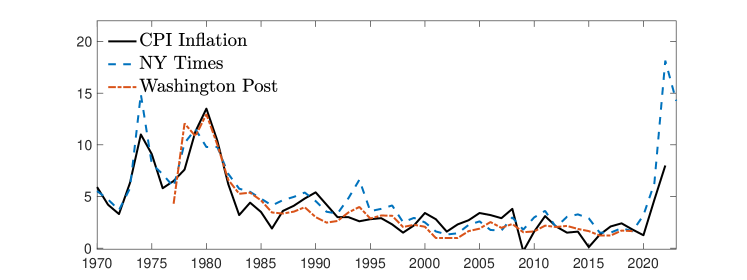
Figure 2: News coverage of inflation is higher in times of high inflation

Notes: The black-solid line shows the annual CPI inflation rate for the US since 1970, the blue-dashed line and the red-dashed-dotted line show the frequency of the word inflation in the New York Times and the Washington post, respectively.

Consistent with this, Bracha and Tang (2023) show that higher inflation rates indeed lead to more media reporting about inflation, and Lamla and Lein (2014) find that more intensive news reporting about inflation improves the accuracy of consumers’ inflation expectations, consistent with agents being more attentive. Schmidt et al. (2023) show that during episodes of intensive newspaper coverage of inflation, news reporting has strong effects on inflation expectations but not during other episodes. Larsen et al. (2021) find that news media coverage predicts households’ inflation expectations, and Nimark and Pitschner (2019) show that major events (such as strong inflation increases) lead to a shift in the news focus towards these events.

2.1 Estimating attention and the attention threshold

In order to estimate the two attention levels $\gamma_{\pi,r}$ for $r\in\{L,H\}$, as well as the attention threshold $\bar{\pi}$, I first rewrite equation (3) as follows:

$$\tilde{E}_{t}\pi_{t+1}=\beta_{0}+\beta_{1}\tilde{E}_{t-1}\pi_{t}+\beta_{2}\left(\pi_{t}-\tilde{E}_{t-1}\pi_{t}\right)+\epsilon_{t},$$ (5)

where $\beta_{0}=(1-\rho_{\pi})\underline{\pi}$ denotes the intercept, $\beta_{1}=\rho_{\pi}$ captures the perceived persistence, and $\tfrac{\beta_{2}}{\beta_{1}}=\gamma_{\pi}$.

I estimate equation (5) using a linear regression model but I allow the coefficients to differ across regimes, whereas the threshold-defining variable is the lagged inflation rate. I allow all coefficients to potentially differ across regimes. The threshold regression is then given by

$$\begin{split}\tilde{E}_{t}\pi_{t+3}&=\mathds{1}_{\pi_{t-1}\leq\bar{\pi}}\left(\beta_{0,L}+\beta_{1,L}\tilde{E}_{t-3}\pi_{t}+\beta_{2,L}\left(\pi_{t}-\tilde{E}_{t-3}\pi_{t}\right)\right)\\ &+(1-\mathds{1}_{\pi_{t-1}\leq\bar{\pi}})\left(\beta_{0,H}+\beta_{1,H}\tilde{E}_{t-3}\pi_{t}+\beta_{2,H}\left(\pi_{t}-\tilde{E}_{t-3}\pi_{t}\right)\right)+\epsilon_{t},\end{split}$$ (6)

where $\mathds{1}_{\pi_{t-1}\leq\bar{\pi}}$ is the indicator function that equals one when inflation in the previous month $\pi_{t-1}$ was below the threshold $\bar{\pi}$ and zero otherwise. The threshold value is then estimated by minimizing the sum of squared residuals obtained for all possible thresholds (see, e.g., Gonzalo and Pitarakis (2002) and Hansen (2011) and the references therein). Note, that I do not impose that the attention level in the regime in which inflation is above the threshold needs to be higher than in the regime with inflation below the threshold. Therefore, the results will serve as a test of the theory outlined above.

Data.

As my measure of inflation expectations, I rely on the Survey of Consumers from the University of Michigan. For my baseline specification, I use average and median household inflation expectations for the period 1978-2023. For the period 2013-2023, I also use individual inflation expectations from the Survey of Consumer Expectations of the New York Fed. Even though I focus on inflation and inflation expectations over one quarter, I use monthly data to increase the number of observations. As a robustness check, however, I also consider expectations at quarterly frequency. One advantage of using quarterly observations is that the Survey of Consumers provides that data going back to 1960Q2. Both surveys ask consumers for their price growth expectations one-year ahead: $\tilde{E}_{t}\pi_{t+12}$. I compute one-quarter-ahead forecasts by dividing the one-year-ahead forecasts by four: $\tilde{E}_{t}\pi_{t+3}\equiv\frac{\tilde{E}_{t}\pi_{t+12}}{4}$. Using $\tilde{E}_{t}\pi_{t+3}\equiv\left[\left(1+{\tilde{E}_{t}\pi_{t+12}}\right)^{\frac{1}{4}}-1\right]$ instead does not change the results. Computing one-quarter-ahead expectations allows me to compare the results directly to the model which is calibrated at quarterly frequency. For actual inflation, I use the monthly CPI inflation rate from the FRED database and to be consistent with the model, I focus on quarter-on-quarter inflation: $\pi_{t}\equiv\frac{P_{t}-P_{t-3}}{P_{t-3}}$.

Estimation results.

Table 1 shows the estimation results. For the baseline specification where I use mean expectations, I estimate an attention threshold of 3.98%. Attention in the regime in which inflation is below this threshold is $\widehat{\gamma}_{\pi,L}=0.18$, and attention in the high-inflation regime is equal to $\widehat{\gamma}_{\pi,H}=0.36$. Thus, attention in the high-inflation regime is higher than in the low-inflation regime, as predicted by the theory. In fact, attention is twice as high in the regime with inflation above the threshold compared to attention in the regime with inflation below the threshold. I therefore refer to the regime with inflation above the threshold as the high-attention regime. The threshold value of 3.98% implies that the US economy spent about 31% of the time in the period 1978-2023 in the high-attention regime. Most recently, inflation exceeded this threshold in early 2021. Google searches also started to increase shortly after that time (see Figure 1 in the Introduction). The results for median expectations are similar. The main difference is that attention in both regimes tends to be somewhat lower when using median expectations and the attention threshold higher. In both cases, the null hypothesis that the two attention levels across regimes are equal is clearly rejected ($p$-values of 0.000 in both cases, see last column).

Table 1: Estimated attention levels and the attention threshold

	Threshold $\bar{\pi}$	Low Attention $\widehat{\gamma}_{\pi,L}$	High Attention $\widehat{\gamma}_{\pi,H}$	$p$-val. $\gamma_{\pi,L}=\gamma_{\pi,H}$
Mean exp.	3.98%	0.18	0.36	0.000
s.e.		(0.013)	(0.037)
Median exp.	4.41%	0.16	0.23	0.000
s.e.		(0.013)	(0.028)
Quarterly freq.	3.21%	0.14	0.38	0.000
s.e.		(0.033)	(0.076)

Notes: This table shows the results from regression (6), where $\bar{\pi}$ denotes the estimated threshold, $\widehat{\gamma}_{\pi,L}$ and $\widehat{\gamma}_{\pi,H}$ the estimated attention levels when inflation is below or above the threshold, respectively. The last column shows the $p$-value for the null hypothesis that the two attention levels are equal. The upper half of the table presents the results when using average expectations, and the lower half when using median expectations. Standard errors are robust with respect to heteroskedasticity.

The last two rows in Table 1 show the results when using observations at quarterly frequency for the period 1960Q2-2023Q2. We see that the estimated threshold is somewhat lower at 3.21%. The estimated attention levels within regime are very similar to my baseline specification and again, the difference in attention across regimes is highly statistically significant.

The estimated perceived persistence coefficients for my baseline specification, $\beta_{1,L}$ and ${\beta}_{1,H}$, are $\widehat{\beta}_{1,L}=0.74$ and $\widehat{\beta}_{1,H}=0.87$, respectively. These estimates are within the 90% confidence intervals of Benati (2008) who estimates inflation persistence in the Great Inflation period for the US to be equal to 0.77, and 0.49 for the Post-Volcker stabilization period. Thus, inflation persistence is higher in times of higher inflation—or, in my case, in times of higher attention.

When I use the current inflation rate rather than the lagged inflation rate as the threshold-defining variable, I find practically identical results. Attention is 0.18 when inflation is below 4% and increases to 0.36 when inflation is above 4%.

When using individual consumer inflation expectations from the Survey of Consumer Expectations, I obtain similar results even though this survey is only available since 2013. When lagged inflation is below the threshold of 4%, I estimate an attention level of 0.21. When inflation was above the threshold, attention doubles to 0.4, and I reject the nullhypothesis that the two estimates are equal ($p$-value of 0.000).

News coverage of inflation is also substantially higher in times inflation is above the attention threshold. I find that the average frequency of the word “inflation” is 2.7 times as high for the New York Times and 2.9 times as high for the Washington Post when CPI inflation is above 4% in that year compared to years in which CPI inflation is below 4%.

My estimated attention threshold is slightly higher than the one estimated in Korenok et al. (2022). They estimate for the US that once inflation exceeds the threshold of 3.55% that attention—measured using Google searches of inflation—increases with inflation whereas it does not below the threshold. One reason why I find a higher threshold could be that people might start to google for information about inflation at lower levels of inflation already, but only start incorporating that information in their expectations once inflation further increases. Additionally, I focus on the time starting in 1978, whereas their sample is restricted to 2004-2022 because the Google search data is not available for years before 2004. They also consider news coverage of inflation, and in that case, they estimate a threshold between 3.77-3.94%, which is very close to the threshold I estimate. Overall my results align with their findings, and my approach provides a quantification of the threshold and the attention levels in a way that is directly applicable to standard macroeconomic models, as we will see in the next section.

Attention changes within regime.

In Table 1 we saw that attention increases strongly when inflation exceeds the threshold of 4%. But what about changes within regime? To look at this, I estimate a whole time series of attention. In particular, I estimate equation (5) using a rolling-window approach, where each window has a length of one year. I denote the estimated time series of attention parameters by $\widehat{\gamma}_{\pi,t}$, and I compute the window-specific average of the monthly quarter-on-quarter inflation rate, $\bar{\pi}_{t}$. To then test whether attention within regime is higher when inflation is higher, I estimate the following regression

$$\widehat{\gamma}_{\pi,t}=\delta_{0}+\delta_{1}\mathds{1}_{\bar{\pi}_{t}\geq 4}+\delta_{2}\bar{\pi}_{t}+\delta_{3}\mathds{1}_{\bar{\pi}_{t}\geq 4}\bar{\pi}_{t}+\varepsilon_{t},$$ (7)

where $\mathds{1}_{\bar{\pi}_{t}\geq 4}$ is an indicator that equals one when average inflation in period $t$ is above 4% and zero otherwise. Thus, $\delta_{1}$ tells us the difference of attention across regimes, $\delta_{2}$ the effect of inflation on attention and $\delta_{3}$ the additional effect of inflation on attention in the high-inflation regime.

The first row in Table 2 shows the results. We see that attention is significantly higher in the higher-inflation regime, as indicated by the estimate of $\delta_{1}$. Yet, inflation does not have any additional significant effect on attention when accounting for the threshold, as depicted by the last two columns.

As a robustness check, I also estimate

$$\widehat{\gamma}_{\pi,t}=\delta_{0}+\delta_{1}\mathds{1}_{\bar{\pi}_{t}\geq 4}+\delta_{2}\pi_{t-1}+\delta_{3}\mathds{1}_{\pi_{t-1}\geq 4}\pi_{t-1}+\varepsilon_{t},$$ (8)

where I use lagged inflation as the independent variable rather than average inflation. The lower part of Table 2 shows that the results are robust. Once I control for the inflation threshold, I do not find any evidence for a positive relationship between inflation and attention on top of the attention shift across regimes.

Table 2: Attention changes within regime

	$\widehat{\delta}_{1}$	$\widehat{\delta}_{2}$	$\widehat{\delta}_{3}$
Regression (7)	$0.393^{**}$	0.053	-0.079
s.e.	(0.192)	(0.047)	(0.051)
Regression (8)	$0.119^{*}$	-0.010	0.010
s.e.	(0.0641)	(0.0141)	(0.0141)

Notes: This table shows the results from regression (7) (upper half of the table) and from regression (8) (lower half of the table). Standard errors are robust with respect to heteroskedasticity and serial correlaton (Newey and West (1987) with 12 lags). Significance levels: ^∗: $p$-value $<$ 0.1, ^∗∗: $p$-value $<$ 0.05, ^∗∗∗: $p$-value $<$ 0.01.

Covid.

When focusing on the sample from 2017 until 2023, I estimate an attention threshold of 3.63%, and attention levels of $\widehat{\gamma}_{\pi,L}=0.03$ and $\widehat{\gamma}_{\pi,H}=0.25$. The very low attention level before the outbreak of the Covid-19 pandemic confirms the findings in Pfäuti (2023) that attention to inflation was at a historical low at the time. When imposing the threshold at 4% (rather than estimating it), attention in the higher regime equals 0.28 and 0.04 in the low regime.

Figure 3 shows news coverage of inflation in the New York Times for the period 2019 until July 2023 at monthly frequency (blue-dashed line) together with monthly year-on-year CPI inflation. The figure shows the strong positive correlation of 0.85 between inflation and news coverage, and that at the peak, news coverage of inflation quintupled from its pre-pandemic level. Consistent with the theory, news coverage lags inflation slightly (the correlation between news coverage and lagged inflation is slightly higher than the one with current inflation, 0.9 instead of 0.85). The correlation of news coverage with Google searches is 0.94 for the period 2017-2023, further supporting the assumption that news coverage is highly correlated with the public’s attention to inflation.

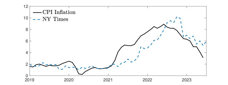
Figure 3: News coverage of inflation during Covid

Notes: The black-solid line shows the monthly year-on-year CPI inflation rate for the US and the blue-dashed line the frequency of the word inflation in the New York Times, normalized to have the same standard deviation as CPI inflation.

Heterogeneity.

So far, I mainly focused on average (and median) expectations. I now test whether the attention threshold and the different attention levels depend on people’s gender or their age. As documented in D’Acunto et al. (2021), gender and gender roles (e.g., with respect to grocery shopping) play a big role in explaining differences in how men and women form their inflation expectations. I find that men have a higher attention threshold than women (4.4% vs. 3.9%), indicating that women increase their attention somewhat earlier than men. This might be explained by the fact that women are more likely to go grocery shopping than men (D’Acunto et al., 2021) and therefore, experience price changes more directly than men. I further find that the threshold for younger people (aged 18-34) is lower than for older people (4.44% vs. 6.8% for people aged between 35 and 54, and 5.7% for people aged older than 55), but that their attention levels tend to be lower overall (0.21 vs. 0.24 below the threshold and 0.41 vs. 0.74 above it).

3 A Monetary Model with Varying Attention

This section presents the monetary model which builds on the textbook New Keynesian model (Woodford, 2003; Galí, 2015) but households and firms pay only limited attention to inflation and the output gap.

3.1 Households

There is a representative household obtaining utility from consumption and disutility from working, with lifetime utility

$$\tilde{E}_{0}\sum_{t=0}^{\infty}\beta^{t}Z_{t}\left[\frac{C_{t}^{1-\sigma}}{1-\sigma}-\Xi\frac{H_{t}^{1+\nu}}{1+\nu}\right],$$ (9)

where $C_{t}$ is consumption of the final good, $H_{t}$ is hours worked, $\beta$ is the household’s time discount factor, and $\tilde{E}_{t}$ denotes the household’s subjective expectations operator based on information available in period $t$. $Z_{t}$ are exogenous preference shocks. The parameters $\sigma$ and $\nu$ pin down the relative risk aversion and the inverse Frisch labor elasticity, respectively. $\Xi$ is the utility weight on hours worked.

Households maximize their lifetime utility subject to the flow budget constraints

$$C_{t}+B_{t}=w_{t}H_{t}+\frac{1+i_{t-1}}{1+\pi_{t}}B_{t-1}+\frac{T_{t}}{P_{t}},\quad\text{ for all }t,$$ (10)

where $B_{t}$ is the real value of government bonds, $w_{t}$ the real wage, $\pi_{t}$ is the net inflation rate, and $i_{t}$ the nominal interest rate. $T_{t}$ denotes lump-sum taxes and transfers from the government.

Maximizing (9) subject to (10) yields the Euler equation

$$Z_{t}C_{t}^{-\sigma}=\beta(1+i_{t})\tilde{E}_{t}\left[Z_{t+1}C_{t+1}^{-\sigma}\frac{1}{1+\pi_{t+1}}\right],$$ (11)

and the labor-leisure condition

$$w_{t}C_{t}^{-\sigma}=\Xi H_{t}^{\nu}.$$ (12)

3.2 Firms

The firm sector is held by risk-neutral managers that discount future profits by $\beta$ and they have a mass of zero, such that their consumption is 0 and all their profits go to the households, as in Bayer et al. (2022).

Final good producer.

There is a representative final good producer that aggregates the intermediate goods $Y_{t}(j)$ to a final good $Y_{t}$, according to

$$Y_{t}=\left(\int_{0}^{1}Y_{t}(j)^{\frac{\epsilon-1}{\epsilon}}dj\right)^{\frac{\epsilon}{\epsilon-1}},$$ (13)

with $\epsilon>1$. Nominal profits are given by $P_{t}\left(\int_{0}^{1}Y_{t}(j)^{\frac{\epsilon-1}{\epsilon}}dj\right)^{\frac{\epsilon}{\epsilon-1}}-\int_{0}^{1}P_{t}(j)Y_{t}(j)dj,$ and profit maximization gives rise to the demand for each variety $j$:

$$Y_{t}(j)=\left(\frac{P_{t}(j)}{P_{t}}\right)^{-\epsilon}Y_{t}.$$ (14)

Thus, demand for variety $j$ is a function of its relative price, the price elasticity of demand $\epsilon$ and aggregate output $Y_{t}$. The aggregate price level is given by

$$P_{t}=\left(\int_{0}^{1}P_{t}(j)^{1-\epsilon}dj\right)^{\frac{1}{1-\epsilon}}.$$ (15)

Intermediate producers.

Intermediate producer of variety $j$ produces output $Y_{t}(j)$ using labor $H_{t}(j)$ as its only input

$$Y_{t}(j)=H_{t}(j).$$ (16)

All intermediate producers pay the same wage $w_{t}$ and a sales tax (or subsidy) $\tau_{t}$, which in steady state is set such that profits in steady state are 0. These taxes are given back to firms in a lump-sum fashion, denoted $t^{F}_{t}(j)$. Taxes are assumed to be constant in the efficient economy, i.e., absent price rigidities, but fluctuate around their steady state in the economy with price rigidities in order to give rise to exogenous cost-push shocks.

Each intermediate firm has two managers: one is responsible for the firm’s forecasts and the other manager sets the price of firm $j$ given these forecasts, similar to the setup in, e.g., Adam and Padula (2011) or in section V of Angeletos and La’o (2010). I discuss here the problem of the price setter and discuss the forecaster’s problem later.

When adjusting the price, the firm is subject to a Rotemberg (1982) price-adjustment friction. Their per-period profits (in real terms) are given by

$$(1-\tau_{t})P_{t}(j)\left(\frac{P_{t}(j)}{P_{t}}\right)^{-\epsilon}\frac{Y_{t}}{P_{t}}-w_{t}H_{t}(j)-\frac{\psi}{2}\left(\frac{P_{t}(j)}{P_{t-1}(j)}-1\right)^{2}Y_{t}+t^{F}_{t}(j),$$ (17)

where $\psi\geq 0$ captures the price-adjustment cost parameter. They set prices to maximize

$$Profits_{0}(j)=\tilde{E}^{j}_{0}\sum\limits_{t=0}^{\infty}\beta^{t}\left[(1-\tau_{t})P_{t}(j)\left(\frac{P_{t}(j)}{P_{t}}\right)^{-\epsilon}\frac{Y_{t}}{P_{t}}-mc_{t}H_{t}(j)-\frac{\psi}{2}\left(\frac{P_{t}(j)}{P_{t-1}(j)}-1\right)^{2}Y_{t}+t^{F}_{t}(j)\right],$$

where $mc_{t}=w_{t}$ denotes the real marginal cost which is the same for every firm. Using the production function to substitute for $H_{t}(j)$ and the demand for firm $j$’s product from the final goods producer, the corresponding first order condition is then given by

$$(1-\tau_{t})(\epsilon-1)P_{t}(j)^{-\epsilon}\frac{Y_{t}}{P_{t}^{1-\epsilon}}= \epsilon mc_{t}\left(\frac{P_{t}(j)}{P_{t}}\right)^{-\epsilon-1}\frac{Y_{t}}{P_{t}}-\psi\left(\frac{P_{t}(j)}{P_{t-1}(j)}-1\right)\frac{Y_{t}}{P_{t-1}(j)}$$

$$+\beta\psi\tilde{E}^{j}_{t}\left[\left(\frac{P_{t+1}(j)}{P_{t}(j)}-1\right)\frac{P_{t+1}(j)}{P_{t}(j)}\frac{Y_{t+1}}{P_{t}(j)}\right].$$

Defining $T_{t}\equiv 1-\tau_{t}$, it follows that after a linearization around the zero-inflation steady state, firm $j$ sets its price according to

$$\widehat{p}_{t}(j)=\frac{1}{\psi+\epsilon}\left[\psi\widehat{p}_{t-1}+\epsilon\left(\widehat{mc}_{t}-\widehat{T}_{t}+\widehat{p}_{t}\right)+\beta\psi\tilde{E}^{j}_{t}\pi^{j}_{t+1}\right],$$ (18)

where hatted variables denote log deviations of the respective variables from their steady state values (see Appendix C for all derivations). Therefore, prices may only differ across firms $j$ due to differences in forecasts $\tilde{E}^{j}_{t}\pi^{j}_{t+1}$.

Government.

The government imposes a sales tax $\tau_{t}$ on sales of intermediate goods, issues nominal bonds, and pays lump-sum taxes and transfers $T_{t}$ to households and $t^{F}_{t}(j)$ to firms. The real government budget constraint is given by

$$B_{t}=B_{t-1}\frac{1+i_{t-1}}{\Pi_{t}}+\frac{T_{t}}{P_{t}}-\tau Y_{t}+t^{f}_{t}.$$

Lump-sum taxes and transfers are set such that they keep real government debt constant at the initial level $B_{-1}/P_{-1}$, which I set to zero.

The monetary authority sets the nominal interest rate, according to a (linearized) Taylor rule:

$$\tilde{i}_{t}=\rho_{i}\tilde{i}_{t-1}+(1-\rho_{i})\left(\phi_{\pi}\pi_{t}+\phi_{x}\widehat{x}_{t}\right),$$ (19)

where $\tilde{i}_{t}$ denotes the nominal interest rate in deviations from its steady state, $\rho_{i}$ captures interest-rate smoothing, $\phi_{\pi}$ and $\phi_{x}$ pin down the response coefficients with respect to inflation and the output gap, respectively.

3.3 Subjective expectations under limited attention

Households.

Households believe that consumption and inflation both follow a random walk:

$$\pi_{t} =\pi_{t-1}+\nu_{\pi,t}$$

$$\widehat{c}_{t} =\widehat{c}_{t-1}+\nu_{c,t},$$

where $\nu_{\pi,t}$ and $\nu_{c,t}$ are normally distributed with mean zero, time-invariant standard deviations and independent from each other. The random walk assumption ensures that long-run expectations align with the actual long-run variables. They observe all aggregate shocks perfectly.

At the time the household forms her expectations about future consumption and inflation, she does not perfectly observe their current realizations. This assumption could capture that the household is not at all times perfectly monitoring all consumption expenditures of the members of the household and that inflation is not perfectly observable in real time. Instead of observing consumption and inflation perfectly, the household only receives noisy signals of the form

$$s_{\pi,t} =\pi_{t}+\varepsilon_{\pi,r,t}$$

$$s_{c,t} =\widehat{c}_{t}+\varepsilon_{c,t},$$

with normally distributed noise terms $\varepsilon_{\pi,r,t}$ and $\varepsilon_{c,t}$. Following the attention choice problem outlined in Section 2, the noise variance regarding inflation $\varepsilon_{\pi,r,t}$ is smaller in the $H$ regime, reflecting the higher attention in that regime.

As detailed in Appendix C, potential output, i.e., output under flexible prices, is constant and consumption in log-deviations from steady state is equal to the output gap in equilibrium, $\widehat{c}_{t}=\widehat{x}_{t}$. It follows that if we assume initial values $\tilde{E}_{-1}\widehat{c}_{0}=\tilde{E}_{-1}\widehat{x}_{0}$, we have $\tilde{E}_{t}\widehat{c}_{t+1}=\tilde{E}_{t}\widehat{x}_{t+1}$ for all $t$. This holds true, even if the household does not know that the two are equal in equilibrium.

Expectations about the output gap, $\widehat{x}_{t}$, then evolve as follows:

$$\tilde{E}_{t}\widehat{x}_{t+1}=\tilde{E}_{t-1}\widehat{x}_{t}+\gamma_{x}\left(\widehat{x}_{t}-\tilde{E}_{t-1}\widehat{x}_{t}\right),$$ (20)

where $\tilde{E}_{t}\widehat{x}_{t+1}$ denotes the agent’s expectations of the one-period-ahead output gap. The parameter $\gamma_{x}$ denotes the optimal level of attention to the output gap, based on the agent’s subjective model of how the output gap evolves. A higher $\gamma_{x}$ denotes a higher attention level. If $\gamma_{x}=0$, the agent is completely inattentive and just sticks to her prior belief $\tilde{E}_{t-1}\widehat{x}_{t}$, whereas $\gamma_{x}=1$ captures the case of full attention in which case the agent believes $\tilde{E}_{t}\widehat{x}_{t+1}=\widehat{x}_{t}$, which is the full-information belief of someone who believes that the output gap follows a random walk. As I discuss in more detail in the calibration section later on, I do not find any differences in attention to unemployment changes (which I use as a proxy for the output gap) in the data. I therefore impose that attention to the output gap, $\gamma_{x}$, does not change across regimes.

Inflation expectations follow the law of motion derived in equation (4) for $\rho_{\pi}=1$, so that they are given by

$$\tilde{E}_{t}\pi_{t+1}=\begin{cases}\tilde{E}_{t-1}\pi_{t}+\gamma_{\pi,L}\left(\pi_{t}-\tilde{E}_{t-1}\pi_{t}\right),\text{ when }\pi_{t-1}<\bar{\pi}\\ \tilde{E}_{t-1}\pi_{t}+\gamma_{\pi,H}\left(\pi_{t}-\tilde{E}_{t-1}\pi_{t}\right),\text{ when }\pi_{t-1}>\bar{\pi},\end{cases}$$ (21)

where $\gamma_{\pi,r}$ captures the optimal level of attention to inflation in regime $r\in\{L,H\}$, depending on the respective cost of information $\frac{1}{\lambda_{r}}$. I abstract from noise shocks and instead assume that the signal the household receives is exactly equal to the variable’s realization in that period, but the household does not know this and acts as if there was noise.

Firm managers.

Since there are no idiosyncratic shocks, I assume that the forecasting manager of firm $j$ uses expectations about aggregate inflation to form her expectations about firm $j$’s future price change, i.e., $\tilde{E}^{j}_{t}\pi_{t+1}(j)=\tilde{E}^{j}_{t}\pi_{t+1}$. Forecasting managers hold the same subjective expectations as households, consistent with McClure et al. (2022) who show that managers and non-managers hold similar average inflation and unemployment expectations and respond similarly to information treatments. Since I abstract from noise shocks, all forecasters receive the same signal about current inflation, from which it follows that $\tilde{E}^{j}_{t}\pi_{t+1}(j)=\tilde{E}^{j}_{t}\pi_{t+1}=\tilde{E}_{t}\pi_{t+1}$.

Given these assumptions, equation (18) can be written as

$$\pi_{t}=\frac{\epsilon}{\psi}\left(\widehat{mc}_{t}-\widehat{T}_{t}\right)+\beta\tilde{E}_{t}\pi_{t+1}.$$ (22)

From the labor-leisure equation and the production function, we have $\widehat{mc}_{t}=\left(\sigma+\nu\right)\widehat{y}_{t}$, and since potential output is constant we have $\widehat{y}_{t}=\widehat{x}_{t}$. Defining cost-push shocks as $u_{t}\equiv-\frac{\epsilon}{\psi}\widehat{T}_{t}$ and $\kappa\equiv\frac{\epsilon}{\psi}\left(\sigma+\nu\right)$, we arrive at the linearized New Keynesian Phillips Curve under subjective expectations:

$$\pi_{t}=\beta\tilde{E}_{t}\pi_{t+1}+\kappa\widehat{x}_{t}+u_{t}.$$ (23)

3.4 Equilibrium

The model can then be summarized by three equilibrium equations when expressed in log-deviations from the zero-inflation steady state (see Appendix C):

$$\pi_{t} =\beta\tilde{E}_{t}\pi_{t+1}+\kappa\widehat{x}_{t}+u_{t},$$ (24)

$$\widehat{x}_{t} =\tilde{E}_{t}\widehat{x}_{t+1}-\varphi\left(\tilde{i}_{t}-\tilde{E}_{t}\pi_{t+1}-r^{*}_{t}\right),$$ (25)

$$\tilde{i}_{t} =\rho_{i}\tilde{i}_{t-1}+(1-\rho_{i})\left(\phi_{\pi}\pi_{t}+\phi_{x}\widehat{x}_{t}\right),$$ (26)

as well as the two law of motions for output gap expectations and inflation expectations, equations (20) and (21). Equation (24) is the New Keynesian Phillips curve, representing the supply side of the economy, and equation (25) denotes the aggregate Euler (or IS) equation, which together with monetary policy (equation (26)) pins down aggregate demand. $\varphi>0$ measures the real rate elasticity of output, and $r^{*}_{t}$ is the natural interest rate. The natural interest rate is the real rate that prevails in the economy with fully flexible prices, and solely depends on the exogenous shocks $Z_{t}$. It follows an AR(1) process with persistence $\rho_{r}\in[0,1]$ and innovations $\varepsilon^{r}\sim i.i.N.(0,\sigma^{2}_{r}),$ independent of $\varepsilon^{u}$. I will refer to shocks to $r^{*}_{t}$ as demand shocks. The nominal interest rate $\tilde{i}_{t}$ and the natural rate are both expressed in absolute deviations of their respective steady state values, $\underline{i}$ and $\underline{r}^{*}$, with $\underline{i}=\underline{r}^{*}$, as the model is linearized around the zero-inflation steady state.

4 Inflation Surges

In this section, I show how the model with two inflation-attention regimes can jointly generate persistent heightened inflation periods and forecast error dynamics that mirror the empirically-observed patterns during the recent high-inflation period in the United States. I find that cost-push shocks are especially inflationary in times of loose monetary policy and that this state dependency is only present in the economy with the attention threshold. Additionally, I show that even relatively small shocks to demand and supply simultaneously can trigger large inflation surges in the model with two attention regimes, whereas inflation would stay relatively low absent the regime change or when only demand or only supply shocks would hit the economy. Before going into these numerical results, however, I use a stylized version of my model economy to illustrate how the attention threshold alters the inflation dynamics.

4.1 An Illustrative Example

To provide intuition how the attention threshold may trigger self-reinforcing inflation surges, I start with a stylized version of the model. In particular, I assume that agents are completely inattentive to the output gap, i.e., $\gamma_{x}=0$, and that the Taylor rule is given by $\tilde{i}_{t}=\phi_{\pi}\pi_{t}$ with $\phi_{\pi}>1$. For readability, I set the interest-rate elasticity $\varphi$ to 1.

The economy starts in the steady state, with $u_{0}=0$, $r^{*}_{0}=0$ and prior expectations are at their long-run averages of 0: $\tilde{E}_{-1}\pi_{0}=0$ and $\tilde{E}_{-1}\widehat{x}_{0}=0.$ The aggregate supply (AS) equation—captured by the Phillips Curve—in this initial period is then given by

$$AS_{0}:\quad\pi_{0}=\frac{\kappa}{1-\beta\gamma_{\pi,L}}\widehat{x}_{0},$$ (27)

and aggregate demand (AD), which follows from combining the Taylor rule with the aggregate Euler (or IS) equation, is given by

$$AD_{0}:\quad\pi_{0}=-\frac{1}{\phi_{\pi}-\gamma_{\pi,L}}\widehat{x}_{0}.$$ (28)

Panel (a) in Figure 4 depicts this initial situation graphically. Inflation and the output gap are both at their steady state values of 0 and therefore, below the inflation attention threshold $\bar{\pi}$.

Figure 4: An illustrative example

(a) Steady state	(b) Cost-push shock hits: AS shifts up
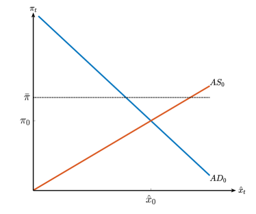
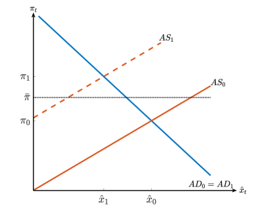
(c) AS: further up and steeper	(d) AD: out and steeper

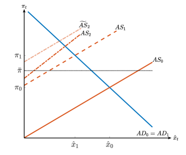
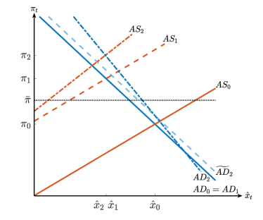
Notes: Panel (a) shows the initial situation in period 0 when the economy is in the steady state. In period 1, a positive cost-push shock hits the economy, leading to an upward shift of the AS curve (panel (b)). In period 2, the AS curve shifts further up (shift from $AS_{1}$ to $\widetilde{AS}_{2}$) and the curve becomes steeper (rotation from $\widetilde{AS}_{2}$ to $AS_{2})$, shown in panel (c). Simultaneously, the AD curve shifts out (shift from $AD_{1}$ to $\widetilde{AD}_{2}$) and becomes stepper (rotation from $\widetilde{AD}_{2}$ to $AD_{2}$), as shown in panel (d). The black-dotted line at $\bar{\pi}$ depicts the inflation attention threshold.

In period 1, a positive cost-push shock hits and I assume that it persists for two periods: $u_{1}=u_{2}>0$ and returns to zero afterwards, $u_{t}=0$ for $t\geq 3$. The AS and AD equations are now given by

$$AS_{1}:\quad \pi_{1}=\frac{\kappa}{1-\beta\gamma_{\pi,L}}\widehat{x}_{1}+\frac{1}{1-\beta\gamma_{\pi,L}}u_{1}$$

$$AD_{1}:\quad \pi_{1}=-\frac{1}{\phi_{\pi}-\gamma_{\pi,L}}\widehat{x}_{1}.$$

This situation is shown in Panel (b) of Figure 4. The cost-push shock shifts the AS curve up along the AD curve. The resulting equilibrium is characterized by output below potential, i.e., a negative output gap, and positive inflation. The increase in inflation is assumed to be relatively large, such that inflation exceeds the threshold.

Due to the increase in inflation in period 1, firms enter the second period with positive prior inflation expectations: $\tilde{E}_{1}\pi_{2}=\gamma_{\pi,L}\pi_{1}>0$. These higher prior expectations together with the still ongoing cost-push shock shift the AS curve further up. This shift is illustrated in panel (c) of Figure 4 by the $\widetilde{AS}_{2}$ curve, which is given by

$$\widetilde{AS}_{2}:\quad\pi_{2}=\frac{\kappa}{1-\beta\gamma_{\pi,L}}\widehat{x}_{2}+\underbrace{\frac{1}{1-\beta\gamma_{\pi,H}}u_{2}+\frac{\beta(1-\gamma_{\pi,H})\gamma_{\pi,L}}{1-\beta\gamma_{\pi,H}}\pi_{1}}_{\text{Intercept}>0}.$$

The terms denoted “Intercept” capture this shift in the AS curve. Since inflation in the previous period exceeded the attention threshold, attention is now higher. This increase in attention leads to an unambiguously stronger effect of the cost-push shock compared to the case in which attention would have remained constant:

$$\frac{1}{1-\beta\gamma_{\pi,H}}u_{2}>\frac{1}{1-\beta\gamma_{\pi,L}}u_{2}.$$

The effect of the increase in firm managers’ prior on inflation in the second period, however, is smaller at the higher attention level. There are two counteracting forces. First, the increase in attention means that firm managers now update their expectations more strongly and put less weight on their prior expectations. This per se leads to a smaller effect. Second, the higher prior increases overall inflation expectations which, ceteris paribus, increases current inflation. But because inflation expectations are discounted by $\beta\leq 1$, the first effect dominates. Therefore, the shift in the AS curve due to the higher prior expectations is smaller at higher attention levels. Quantitatively, however, these differences are very small as $\beta\approx 1$. In fact, if $\beta=1$, the change in attention has no effect on the shift due to higher prior expectations, and therefore, the total shift of the AS curve is unambiguously higher when attention is higher, due to stronger effect of the cost-push shock.

The shift of the AS curve to $\widetilde{AS}_{2}$, however, is only part of the story. What I ignored so far is that the increase in attention also increases the slope of the AS curve. That is, the Phillips Curve becomes steeper in periods of high attention—a dynamic non-linearity. Taking this into account, the AS curve in the second period is given by

$$AS_{2}:\quad\pi_{2}=\underbrace{\frac{\kappa}{1-\beta\gamma_{\pi,H}}}_{\text{Slope}}\widehat{x}_{2}+\frac{1}{1-\beta\gamma_{\pi,H}}u_{2}+\frac{\beta(1-\gamma_{\pi,H})\gamma_{\pi,L}}{1-\beta\gamma_{\pi,H}}\pi_{1}.$$

This steepening of the AS curve is illustrated in panel (c) of Figure 4 by the rotation of the AS curve from $\widetilde{AS}_{2}$ to $AS_{2}$. This steepening of the AS curve eases the inflationary pressures due to the negative output gap. Nevertheless, the steeper AS curve implies that if the AD curve would now shift out, the inflationary effects of this increase in demand would become larger.

It turns out that the higher prior expectations lead to such a demand increase. This is illustrated by $\widetilde{AD}_{2}$ in panel (d) of Figure 4, which is given by

$$\widetilde{AD}_{2}:\quad\pi_{2}=-\frac{1}{\phi_{\pi}-\gamma_{\pi,L}}\widehat{x}_{2}+\frac{(1-\gamma_{\pi,H})\gamma_{\pi,L}}{\phi_{\pi}-\gamma_{\pi,H}}\pi_{1}.$$

The higher prior expectations, ceteris paribus, decrease the real rate which leads to the outward shift of the AD curve. These effects, however, are smaller at higher levels of attention as long as the Taylor principle, $\phi_{\pi}>1$, is satisfied, because in that case the higher inflation rates due to the higher prior expectations are counteracted by a more than one-for-one increase in the nominal rate. If monetary policy is relatively dovish, i.e., $\phi_{\pi}$ is close to 1, these differences are small. Furthermore, since the AD curve is now shifted along a steeper AS curve due to the heightened attention, the inflationary effects of a given shift are larger at the higher level of attention. This also implies that additional demand stimulus—for example, due to loose monetary policy or a fiscal stimulus—would have relatively large inflationary effects.

Additionally, the AD curve also becomes steeper, as illustrated by the rotation from $\widetilde{AD}_{2}$ to $AD_{2}$ in panel (d), where $AD_{2}$ is given by

$$AD_{2}:\quad\pi_{2}=-\frac{1}{\phi_{\pi}-\gamma_{\pi,H}}\widehat{x}_{2}+\frac{(1-\gamma_{\pi,H})\gamma_{\pi,L}}{\phi_{\pi}-\gamma_{\pi,H}}\pi_{1}.$$

This leads to a further increase in inflation, especially now because the AS curve is steeper. In this stylized example, inflation increases substantially from period 1 to period 2 through the change in attention, whereas the output gap remains practically constant. Thus, the attention threshold offers a theory of how inflation surges may occur and exhibit self-reinforcing dynamics without changes in output.

In the third period, when the shock has died out, the AS curve shifts back down. The AS curve is given by

$$AS_{3}:\quad\pi_{3}=\frac{\kappa}{1-\beta\gamma_{\pi,H}}\widehat{x}_{3}+\frac{\beta(1-\gamma_{\pi,H})}{1-\beta\gamma_{\pi,H}}\tilde{E}_{2}\pi_{3}.$$

Due to the positive prior expectations, $\tilde{E}_{2}\pi_{3}>0$, the AS curve does not fully shift back to its initial position but remains above it. Due to the higher steepness of the AD curve, however, the shift in the AS curve leads to a stronger reduction in inflation compared to a flatter AD curve.

While the AS curve comes back down, the AD curve shifts further out due to the positive prior expectations that agents have when going into period 3. The AD curve is given by

$$AD_{3}:\quad\pi_{3}=-\frac{1}{\phi_{\pi}-\gamma_{\pi,H}}\widehat{x}_{3}+\frac{1-\gamma_{\pi,H}}{\phi_{\pi}-\gamma_{\pi,H}}\tilde{E}_{2}\pi_{3}.$$

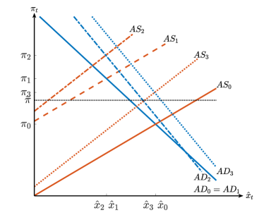
Figure 11: Illustrative example: after the shock has died out

Thus, output recovers more strongly during this disinflationary period than what would be the case absent this shift in the AD curve, and disinflationn occurs more gradually. These results are shown graphically in Figure 11 in Appendix D.

4.2 Large vs. small shocks

Equipped with these theoretical insights, I now move to a numerical analysis of the attention threshold. To do so, I first have to calibrate the model. Following the empirical findings in Section 2, I set $\gamma_{\pi,L}=0.18$ and $\gamma_{\pi,H}=0.36$, and the attention threshold to $\bar{\pi}=4\%$ (annualized). I calibrate the shock volatilities in order to match the finding that the economy spends 31% of the time in the high-attention regime, and I assume that both shocks have the same volatility and persistence. This results in $\sigma_{r}=\sigma_{u}=0.50\%$ and $\rho_{r}=0.8=\rho_{u}=0.8$.

The rest of the calibration is standard. I set the discount factor $\beta$ to target a steady state natural rate of $1\%$ (annualized), the interest-rate sensitivity $\varphi$ to 1, and the slope of the Phillips curve $\kappa$ to 0.057. The Taylor rule coefficients are set to $\rho_{i}=0.7$, $\phi_{\pi}=2$ and $\phi_{x}=0.125$. To calibrate the attention parameter with respect to the output gap $\gamma_{x}$, I follow the same procedure as for inflation but focus on expectations about unemployment changes (see Appendix B.1). This results in $\gamma_{x}=0.24$ when inflation is below 4%, and $\gamma_{x}=0.25$ when inflation is above it. The two estimates are not statistically significant from each other. I therefore impose that $\gamma_{x}$ does not change across regimes and set it to $\gamma_{x}=0.25$.

Figure 5 shows the inflation dynamics following a cost-push shock that pushes inflation in the first period above the attention threshold $\bar{\pi}$ (the red-dashed line shows the inflation response, and the black-dotted line the attention threshold), as well as following a shock that does not push inflation above the threshold (blue-dashed-dotted line).

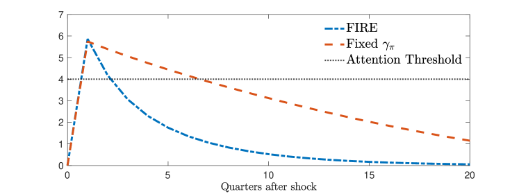
Figure 13: Inflation dynamics under FIRE or absent the attention change

The two cases exhibit quite different inflation dynamics. In response to the relatively small shock, inflation increases on impact and then gradually returns back to its initial value of zero. After the larger shock, however, inflation keeps on increasing for about five periods before it peaks and then starts to decrease thereafter. While this decrease happens relatively fast at first, it slows down once inflation falls back below the attention threshold, and thus, inflation remains elevated quite persistently. The model under FIRE exhibits similar dynamics than the blue line but inflation returns even more quickly to its initial value (see Figure 13 in Appendix D).

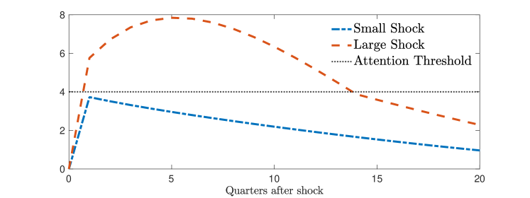
Figure 5: Inflation dynamics

To understand the dynamics in the model with the attention threshold, both regime switches that take place are key. The first regime switch occurs because the shock impulse is large enough to increase inflation above its threshold. Thus, in the second period, agents become more attentive to inflation and hence, increase their inflation expectations more strongly in response to the forecast errors they make. For a given nominal rate, households now perceive the real rate to be lower and thus, increase their consumption in response. The attention regime change also matters for the supply side. Firms increase their inflation expectations more strongly which leads them to increase their prices more strongly. On top of that, the equilibrium inflation response to the cost-push shock for a given state is higher in the high-attention regime:

$$\frac{\partial\pi_{t+j}}{\partial u_{t+j}}\Bigr{|}_{\gamma_{\pi,H}}>\frac{\partial\pi_{t+j}}{\partial u_{t+j}}\Bigr{|}_{\gamma_{\pi,L}}.$$

Hence, inflation keeps on increasing, further fueling higher inflation expectations, leading to additional inflation increases. As the shock slowly dies out, inflation eventually starts to decrease.

The second regime switch—once inflation falls back below the threshold value $\bar{\pi}$—leads to the slow inflation decrease after the initial inflation surge. When the economy enters the low-attention regime, agents decrease their attention to inflation. Thus, they mainly stick to their prior beliefs and only slowly update their expectations. As their priors are now relatively high due to the high inflation period, inflation expectations remain high persistently which hinders actual inflation from decreasing quickly.

Figure 6: Inflation and inflation expectation dynamics

Model

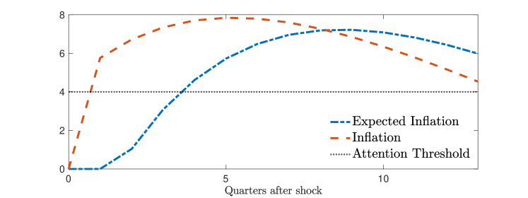
Data

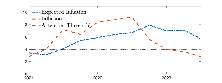
Notes: The upper panel shows the dynamics of inflation and inflation expectations after a cost-push shock that pushes inflation above the attention threshold. The lower panel plots quarter-on-quarter (annualized) CPI inflation and one-quarter-ahead mean inflation expectations for the period 2021-2023, as well as the estimated attention threshold at 4%. In both panels, the inflation expectations are shifted such that the vertical distance between the two gives the respective forecast errors.

To clearly see these patterns of inflation and inflation expectations, the upper panel in figure 6 plots expected and actual inflation, jointly. Inflation expectations are shifted such that the vertical distance between the two lines captures the forecast errors. Initially, expected inflation does not quite catch up with actual inflation, leading to positive forecast errors. After some time—around 8 quarters after the shock—when inflation is already decreasing, expected inflation surpasses actual inflation. Hence, forecast errors become negative.

As the lower panel in figure 6 shows, these patterns are consistent with the recent inflation surge in the US. The figure shows annualized quarter-on-quarter CPI inflation and average inflation expectations from the Michigan Survey for the period from 2021 until 2023Q2. Consistent with the model implications, inflation peaks about a year and a half after its first increase. During this inflation surge, inflation expectations lagged actual inflation. As inflation peaked and began to decline, however, inflation expectations started to surpass actual inflation after about a year and a half after inflation exceeded the attention threshold. Consistent with the model, inflation peaks at a higher value than inflation expectations.

State dependency.

What happens when the cost-push shock occurs at a time of loose monetary policy? Gagliardone and Gertler (2023) argue that easy monetary policy was a key contributor to the recent inflation surge in the US. To model this, I assume that there is an i.i.d. expansionary monetary policy shock at the same time the cost-push shock occurs. Both shocks are such that they increase inflation on impact by 3 percentage points.

Figure 7: Cost-push shocks have larger effects during times of loose monetary policy

(a) Varying attention: $\gamma_{\pi,r}\in\{0.18,0.36\}$	(b) Fixed attention: $\gamma_{\pi}=0.18$
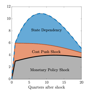
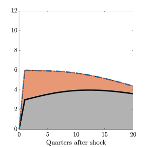
(c) Fixed attention: $\gamma_{\pi}=0.36$	(d) FIRE

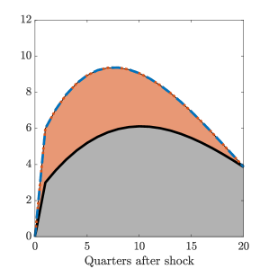
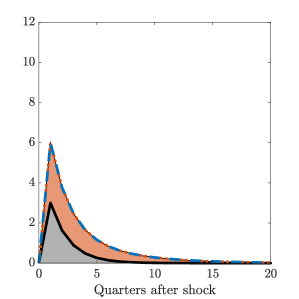
Notes: This figure illustrates the state dependency of cost-push shocks in the economy with the attention threshold. Panel (a) shows the inflation response in the baseline model with the attention threshold, panel (b) shows the case absent the threshold in which attention remains at its low value, panel (c) shows the response in the model with a fixed attention level at the high level of 0.36, and (d) shows the response under FIRE. In all cases, the black-solid line shows the response to a one-time expansionary monetary policy shock in isolation, the orange area shows the response to the cost-push shock, such that the orange-dotted line then shows the sum of the two. The blue-dashed line shows the total response when the two shocks occur simultaneously. The blue-shaded area captures the interaction effect (or the state dependency) of the two shocks.

Figure 7 shows the resulting inflation dynamics in response to these shocks. Panel (a) shows the inflation response in the baseline model with the attention threshold, panel (b) shows the case absent the threshold in which attention remains at its low value, panel (c) the model response when attention is permanently at its high value, and panel (d) shows the response in the model under FIRE. In all cases, the black-solid line shows the response to the monetary policy shock in isolation, the orange area shows the response to the cost-push shock, such that the orange-dotted line then shows the sum of the two. The blue-dashed line shows the total response when the two shocks occur simultaneously. Thus, the blue-shaded area captures the interaction effect of the two shocks, or put differently, the state dependency.

We see from panel (a) that this state dependency is substantial in the model with the attention-regime change but is absent in all other models. At peak, inflation increases by five additional percentage points compared to the two shocks in isolation. The reason for this state dependency is the shift in attention that occurs only when both shocks are present. By entering the high-attention regime, the higher sensitivity of inflation expectations fuel an additional increase in inflation that is not present when attention remains constant.

These effects are absent in the economies without the attention change or under FIRE, even though the initial inflation surge is the same in all three economies. When attention stays low (panel (b)), the feedback effect through the change in inflation expectations is not strong enough to induce further inflation increases, and hence, there is no state dependency. The same is true for the model under rational expectations. Similarly, the model with a constantly-high level of attention does not generate these interaction effects and the inflation peak is below the one in the model with the attention threshold. Thus, accounting for the attention threshold and the increase in attention offers a potential explanation for why inflation may increase more strongly and faster when monetary policy is loose at the time of an inflationary shock.

4.3 What drives inflation surges?

While the debate is still ongoing on what exactly led to the recent inflation surge in the US, I show in this section that high and persistent inflationary episodes may occur even when supply and demand shocks in isolation would only lead to relatively mild inflation rates (see, e.g., Bernanke and Blanchard (2023); Benigno and Eggertsson (2023); Bianchi and Melosi (2022); Di Giovanni et al. (2022); Pflueger (2023); Gagliardone and Gertler (2023) for possible different explanations of the recent inflation dynamics). For this, I simulate the economy for 10,000 periods by randomly drawing demand shocks $\{r^{*}_{t}\}$ and supply shocks $\{u_{t}\}$ and feeding them into the model economy. Figure 8 shows a forty-five year outtake of these simulations. The upper panel shows the inflation dynamics for the case in which the economy is hit by both shocks (blue-solid line), and the cases where the economy is hit only by supply shocks (red-dashed line) or only by demand shocks (black-dashed-dotted line). The lower panel compares the economy with the two attention regimes (blue-solid line) with the model featuring only one attention regime (red-dashed line) and the model under full-information rational expectations (black-dashed-dotted line).

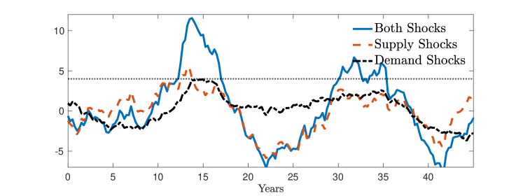
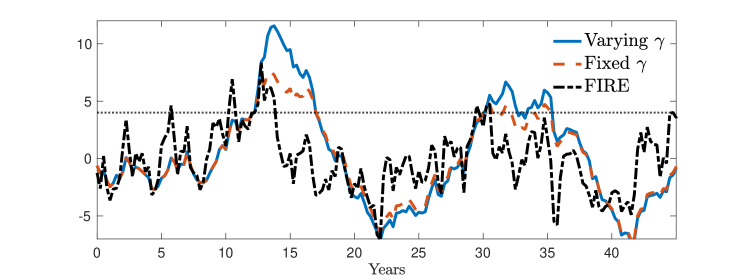
Figure 8: Inflation surges

Notes: The upper panel shows the inflation dynamics for the case in which the economy is hit by both shocks (blue-solid line), and the cases where the economy is hit only by supply shocks (red-dashed line) or only by demand shocks (black-dashed-dotted line). The lower panel compares the economy with the two attention regimes (blue-solid line) with the model featuring only one attention regime (red-dashed line) and the model under full-information rational expectations (black-dashed-dotted line).

In this specific outtake of the simulation, inflation enters the high-attention twice. From the upper panel of Figure 8, we see that these high-inflation episodes are driven by a combination of supply and demand shocks. If only one shock would be hitting the economy in this specific scenario, inflation would exceed the attention threshold only once and only for a relatively short time. However, as illustrated in Figure 5, high-inflation episodes may also arise due to a single shock if the shock is large enough.

The lower panel illustrates how the regime changes exacerbate the inflationary dynamics in two ways. First, by making these high-inflation episodes more long lasting, especially when compared to the economy under full-information rational expectations. This occurs because the increase in attention triggers self-reinforcing inflation and inflation expectation dynamics, thus, keeping inflation higher for longer, as discussed in section 4.2. Second, by amplifying the increase in inflation. The inflation surges are almost twice as high compared to the economy without the change in attention or as in the model under FIRE.

But while the inflation attention threshold exacerbates high inflationary periods, the periods of low inflation (or even deflation) are actually quite similar across models. Thus, the attention threshold introduces an asymmetry: attention increases when inflation is particularly high but not when it is particularly low. This asymmetry leads to a higher average inflation rate. So, the attention threshold not only amplifies inflation fluctuations, but also increases its level. Both of these effects lead to welfare losses, as I discuss next.

5 Welfare Implications

I now characterize the normative implications of the inflation attention threshold and the corresponding changes in attention to inflation. To compare different policy rules, I define welfare as

$$-\frac{1}{2}E_{0}\sum\limits_{t=0}^{\infty}\beta^{t}\left[\pi^{2}_{t}+\Lambda\widehat{x}_{t}^{2}\right],$$ (29)

where $\Lambda$ is the relative weight of the output gap, which I set to $\Lambda=0.007$ as in Adam and Billi (2006). Welfare (29) is obtained by deriving a second-order approximation to the household’s utility function (see, e.g., Woodford (2003)). An implicit assumption here is that the policymaker is paternalistic (Benigno and Paciello, 2014) in the sense that the policymaker evaluates the household’s utility under rational expectations. I further assume that the policy maker is not aware of the private agents’ limited attention and acts as if they hold rational expectations.

Table 3: Monetary policy rules

Nr.	Name	Equation
(1)	Taylor rule with smoothing	$\tilde{i}_{t}=\rho_{i}\tilde{i}_{t-1}+(1-\rho_{i})\left(\phi_{\pi}\pi_{t}+\phi_{x}\widehat{x}_{t}\right)$
(2)	Taylor rule without smoothing	$\tilde{i}_{t}=\phi_{\pi}\pi_{t}+\phi_{x}\widehat{x}_{t}$
(3)	Optimal commitment policy	$\pi_{t}+\tfrac{\Lambda}{\kappa}\left(\widehat{x}_{t}-\widehat{x}_{t-1}\right)=0$
(4)	Optimal discretionary policy	$\pi_{t}+\tfrac{\Lambda}{\kappa}\widehat{x}_{t}=0$
(5)	Strict inflation targeting	$\pi_{t}=0$

When implementing the optimal policy, the policymaker maximizes welfare (29) subject to the private sector’s optimality conditions, given by equations (24)-(25), but as if the private sector’s expectations were rational. As Clarida et al. (1999) show, the optimal policy under commitment is given by

$$\pi_{t}+\tfrac{\Lambda}{\kappa}\left(\widehat{x}_{t}-\widehat{x}_{t-1}\right)=0$$

when agents hold rational expectations. Under discretion, the optimal policy does not take its effects on inflation expectations into account and is then given by

$$\pi_{t}+\tfrac{\Lambda}{\kappa}\widehat{x}_{t}=0.$$

In the following, I compare the welfare implications of these different policy rules and compare them to the Taylor rule (26) as well as to a Taylor rule without interest rate smoothing, i.e., to (26) where $\rho_{i}=0$, as well as to a strict-inflation targeting regime in which inflation is kept at zero at all times. Table 3 summarizes these different policy rules.

I then simulate the economy for 10,000 periods and for the different policy rules. Figure 9 plots welfare (29) for the model with the attention threshold (blue-solid line), with limited attention but absent the attention threshold (red-dashed line) and the model under FIRE (black-dashed-dotted line) for the 5 different policy rules. Panel (a) in Figure 10 shows the respective inflation volatilities, panel (b) the average level of inflation, and panel (c) the frequency of how often inflation is above the threshold of 4%.

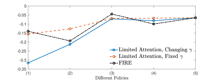
Figure 9: Welfare

Figure 10: Inflation volatility, average inflation and time spent in the high-attention regime

(a) Inflation volatility	(b) Average inflation	(c) Frequency high-attention

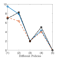
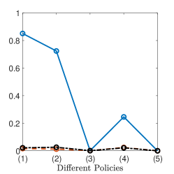
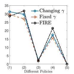
There are two main takeaways from figures 9 and 10. First, following simple Taylor rules (policy rules (1) and (2)) leads to substantially larger welfare losses compared to optimal policy rules or a strict inflation targeting rule in the model with the attention threshold, especially for the case with interest-rate smoothing. The reason is that the economy spends a substantial amount of time in the high-attention regime in which inflation is high and volatile (see panel (c) in figure 10). Due to the asymmetry of the attention threshold the average level of inflation is higher when the economy is in the high-attention regime frequently (panel (b)). This is in stark contrast to the model without the threshold or the one with fully-informed rational agents, where inflation fluctuates symmetrically around zero. Interest rate smoothing introduces additional persistence, such that the periods in the high-attention regime last longer and thus, the average level of inflation as well as its volatility increase.

The second main take away is that neither limited attention nor the attention threshold have large welfare implications, when monetary policy follows one of the rules (3)-(5). In all cases, inflation is relatively stable and fluctuates almost symmetrically around 0, as the economy very rarely stays in the high-attention regime (an exception is the optimal discretion rule (2)). In the case of the strict-inflation targeting regime (5) the inflation volatility is exactly 0. However, in that case, the output gap is more volatile (not shown) such that the overall welfare losses are very similar to the ones under the other policy rules from (3) and (4).

Overall, figures 9 and 10 illustrate that following simple Taylor rules, especially ones with interest-rate smoothing and relatively low inflation-response coefficients, can lead to large welfare losses when the public’s attention to inflation may increase substantially during times of high inflation. Policies that are more hawkish and induce much smaller inflation fluctuations, in contrast, can mitigate the potentially detrimental effects of sudden increases in attention much more effectively, or even prevent these episodes from happening completely.

6 Conclusion

The recent inflation surge in many advanced economies brought inflation back on people’s minds. In this paper, I quantify the inflation attention threshold after which people start to pay more attention to inflation. I estimate this attention threshold to be at an inflation rate of 4% in the United States and that attention doubles from the low-attention regime to the high-attention regime. I estimate these statistics in a way that allows me to directly map the empirical estimates into an otherwise standard New Keynesian model.

Accounting for the inflation attention threshold substantially alters inflation and inflation expectation dynamics in response to shocks. When calibrating the model to match the empirical facts, the model generates inflation and inflation expectation dynamics that are consistent with the ones recently observed in the US.

Accounting for varying attention levels also matters for the models’ normative predictions. Following simple Taylor rules leads to much larger welfare losses compared to optimal policy rules. Such simple policies induce frequent and long-lasting episodes in which attention is heightened which leads to large welfare losses, not only because these episodes increase the overall volatility of inflation, but—due to the asymmetry of the attention threshold—also the average inflation rates.

Appendix A A Limited-Attention Model of Inflation Expectations

In this section, I derive the expectations-formation process under limited attention sketched in Section 2. The agent believes that (demeaned) inflation tomorrow, $\pi^{\prime}$, depends on (demeaned) inflation today, $\pi$, as follows

$$\pi^{\prime}=\rho_{\pi}\pi+\nu,$$

where $\rho_{\pi}\in[0,1]$ denotes the perceived persistence of inflation and $\nu\sim i.i.N.(0,\sigma^{2}_{\nu})$. Inflation in the current period is unobservable, so before forming an expectation about future inflation, the agent needs to form an expectation about today’s inflation. I denote this nowcast $\widetilde{\pi}$, and the resulting forecast about next period’s inflation $\pi^{e}=\rho_{\pi}\widetilde{\pi}$. Given her beliefs, the full-information forecast $\pi^{e*}$ is

$$\pi^{e*}\equiv\rho_{\pi}\pi.$$

But since $\pi$ is not perfectly observable, the actual forecast will deviate from the full-information forecast. Deviating, however, is costly, as this causes the agent to make mistakes in her decisions.

The agent’s choice is not only about how to form her expectations given certain information, but about how to choose this information optimally, while taking into account how this will later affect her forecast. That is, she chooses the form of the signal $s$ she receives about current inflation. Since acquiring information is costly, it cannot be optimal to acquire different signals that lead to an identical forecast. Due to this one-to-one relation of signal and forecast, we can directly work with the joint distribution of $\pi^{e}$ and $\pi$, $f(\pi^{e},\pi)$, instead of working with the signal.

Let $U(\pi^{e},\pi)$ denote the negative of the loss that is incurred when the agent’s forecast deviates from the forecast under full information, and $C(f)$ the cost of information. Then, the agent’s problem is given by

$$\max_{f}\int U(\pi^{e},\pi)f(\pi^{e},\pi)d\pi d\pi^{e}-C(f)$$ (30)

subject to $$\int f(\pi^{e},\pi)d\pi^{e}=g(\pi),\text{ for all }\pi,$$

where $g(\pi)$ is the agent’s prior, which is assumed to be Gaussian; $\pi\sim N\left(\widehat{\pi},\sigma^{2}_{\pi}\right)$. $C(.)$ is the cost function that captures how costly information acquisition is. It is linear in mutual information $I(\pi;\pi^{e})$, i.e., the expected reduction in entropy of $\pi$ due to knowledge of $\pi^{e}$:

$$C(f)=\frac{1}{\lambda}I(\pi;\pi^{e})=\frac{1}{\lambda}\left(H(\pi)-E\left[H(\pi|\pi^{e})\right]\right),$$

where $H(x)=-\int f(x)log(f(x))dx$ is the entropy of $x$ and $\frac{1}{\lambda}$ measures the cost of information.

The objective function $U(.)$ is assumed to be quadratic:

$$U(\pi^{e},\pi)=-\chi\left(\rho_{\pi}\pi-\pi^{e}\right)^{2},$$

where $\chi$ measures the stakes of making a mistake.

In this setup, Gaussian signals are optimal (and in fact the unique solution, see Matějka and McKay (2015)). The optimal signal thus has the form

$$s=\pi+\varepsilon,$$

with $\varepsilon\sim i.i.N.(0,\sigma^{2}_{\varepsilon})$. The problem (30) now reads

$$\max_{\sigma^{2}_{\pi|s}\leq\sigma^{2}_{\pi}}E_{\pi}\left[E_{s}\left[-\chi\rho_{\pi}^{2}\left(\pi-E[\pi|s]\right)^{2}\right]\right]-\frac{1}{\lambda}I(\pi;\pi^{e})=\max_{\sigma^{2}_{\pi|s}\leq\sigma^{2}_{\pi}}\left(-\chi\rho_{\pi}^{2}\sigma^{2}_{\pi|s}-\frac{\frac{1}{\lambda}}{2}log\frac{\sigma^{2}_{\pi}}{\sigma^{2}_{\pi|s}}\right).$$ (31)

The optimal forecast is given by $\pi^{e}=\rho_{\pi}E\left[\pi|s\right]$, and Bayesian updating implies

$$\pi^{e}=\rho_{\pi}\left(1-\gamma\right)\widehat{\pi}+\rho_{\pi}\gamma s,$$ (32)

where $\gamma=1-\frac{\sigma^{2}_{\pi|s}}{\sigma^{2}_{\pi}}\in[0,1]$ measures how much attention the agent pays to inflation, and $\widehat{\pi}$ denotes the prior mean of $\pi$.

An equivalent way of writing $\gamma$ is

$$\gamma=\frac{\sigma^{2}_{\pi}}{\sigma^{2}_{\pi}+\sigma^{2}_{\varepsilon}}.$$ (33)

Now, since the agent chooses the level of attention, we can re-formulate (31) as

$$\max_{\gamma\in[0,1]}\left(-\chi\rho_{\pi}^{2}(1-\gamma)\sigma^{2}_{\pi}-\frac{\frac{1}{\lambda}}{2}log\frac{1}{1-\gamma}\right).$$ (34)

Solving this optimization problem (34) yields the optimal level of attention, presented in Section 2.

Appendix B Appendix to Empirical Section 2

B.1 Unemployment expectations

In order to calibrate the attention parameter with respect to the output gap, $\gamma_{x}$, I use expectations about unemployment changes from the Survey of Consumers. The survey asks households whether they expect unemployment to increase, decrease or to remain about the same over the next twelve months. I follow Carlson and Parkin (1975), Bhandari et al. (2019) and Pfäuti and Seyrich (2023) to translate these categorical unemployment expectations into numerical expectations.

Let $q^{D}_{t}$, $q^{S}_{t}$ and $q^{U}_{t}$ denote the shares reported at time $t$ that think unemployment will go down, stay roughly the same, or go up over the next year, respectively. I assume that these shares are drawn from a cross-sectional distribution of responses that are normally distributed according to $\mathcal{N}\left(\mu_{t},(\sigma_{t})^{2}\right)$ and a threshold $a$ such that when a household expects unemployment to remain within the range $[-a,a]$ over the next year, she responds that unemployment will remain ”about the same”. We thus have

$$q^{D}_{t}=\Phi\left(\frac{-a-\mu_{t}}{\sigma_{t}}\right)\qquad q^{U}_{t}=1-\Phi\left(\frac{a-\mu_{t}}{\sigma_{t}}\right),$$

which after some rearranging yields

$$\sigma_{t} =\frac{2a}{\Phi^{-1}\left(1-q^{U}_{t}\right)-\Phi^{-1}\left(q^{D}_{t}\right)}$$

$$\mu_{t} =a-\sigma_{t}\Phi^{-1}\left(1-q^{U}_{t}\right).$$

This leaves us with one degree of freedom, namely $a$. I follow Pfäuti and Seyrich (2023) and set $a=0.5$ which means that if a household expects the change in unemployment to be less than half a percentage point (in absolute terms), she reports that she expects unemployment to be about the same as it is at the time of the survey. I use data from FRED for the actual unemployment changes and restrict the sample to end in 2019Q4, due to the extreme behavior of unemployment changes with the outbreak of the Covid-19 pandemic.

I then estimate $\gamma_{x}$ separately for whether lagged inflation is above or below the estimated threshold of 4%. This results in estimates $\widehat{\gamma}_{x,L}=0.25$ and $\widehat{\gamma}_{x,H}=0.25$. Thus, there are no differences in attention to unemployment changes across regimes and hence, I impose $\gamma_{x}$ to be the same across regimes in the model.

Appendix C Model Derivations

Derivation of equation (25).

Linearizing the Euler equation (11) yields

$$\widehat{c}_{t}=\tilde{E}_{t}\widehat{c}_{t+1}-\varphi\left(\tilde{i}_{t}-\tilde{E}_{t}\pi_{t+1}-(\widehat{z_{t}}-\tilde{E}_{t}z_{t+1})\right).$$ (35)

The representative household therefore needs to form expectations about future consumption $\tilde{E}_{t}\widehat{c}_{t+1}$, inflation $\tilde{E}_{t}\pi_{t+1}$ and the exogenous preference shock $\tilde{E}_{t}\widehat{z}_{t+1}$. The household holds rational expectations about the shock, so $\tilde{E}_{t}\widehat{z}_{t+1}=E_{t}\widehat{z}_{t+1}$, where $E_{t}(\cdot)$ denotes the rational expectations operator, and since $\widehat{z}_{t}$ follows an AR(1) process with persistence $\rho_{z}$, it follows that $\tilde{E}_{t}\widehat{z}_{t+1}=E_{t}\widehat{z}_{t+1}=\rho_{z}\widehat{z}_{t}$.

Following the discussion in Section 2, the household holds a subjective model of how consumption and inflation evolve. She believes that they both follow a random walk:

$$\pi_{t} =\pi_{t-1}+\nu_{\pi,t}$$

$$\widehat{c}_{t} =\widehat{c}_{t-1}+\nu_{c,t},$$

where $\nu_{\pi,t}$ and $\nu_{c,t}$ are normally distributed with mean zero, time-invariant standard deviations and independent from each other. At the time the household needs to form expectations about future consumption and inflation, she does not perfectly observe their current realizations. This assumption could capture that the household is not at all times perfectly monitoring all consumption expenditures of the members of the household. Instead of observing consumption (and inflation) perfectly, the household only receives noisy signals of the form

$$s_{\pi,t} =\pi_{t}+\varepsilon_{\pi,t}$$

$$s_{c,t} =\widehat{c}_{t}+\varepsilon_{c,t},$$

with normally distributed noise terms $\varepsilon_{\pi,t}$ and $\varepsilon_{c,t}$. As explained in Sections 2 and A, the noise of these signals is endogenous and depends on how attentive the household is. Given these signals, it follows from the (steady state) Kalman filter that optimal updating in regime $r$ is given by

$$\tilde{E}_{t}\pi_{t+1} =\tilde{E}_{t-1}\pi_{t}+\gamma_{\pi,r}\left(\pi_{t}-\tilde{E}_{t-1}\pi_{t}\right)+u_{\pi,t}$$

$$\tilde{E}_{t}\widehat{c}_{t+1} =\tilde{E}_{t-1}\widehat{c}_{t}+\gamma_{c,r}\left(\widehat{c}_{t}-\tilde{E}_{t-1}\widehat{c}_{t}\right)+u_{c,t}.$$

I abstract from noise shocks and therefore impose that $u_{\pi,t}$ and $u_{c,t}$ are zero.

In order to express equation (35) in terms of the output gap, we need to derive the efficient allocation, i.e., the one that prevails in the economy with fully flexible prices. From the production function, we have $Y^{*}_{t}=H^{*}_{t}$. The real wage is constant $w^{*}_{t}=1$. From the labor-leisure equation (12), we get that potential output is therefore also constant and equal to

$$Y^{*}_{t}=\Xi^{-\frac{1}{\nu+\sigma}}.$$ (36)

Thus, potential output in log-deviations is 0. The Euler equation in the flexible-price economy is therefore given by

$$0=-\varphi\left(r_{t}-(\widehat{z_{t}}-\tilde{E}_{t}z_{t+1})\right).$$

Since the natural rate is defined as the real rate that prevails under flexible prices, $r_{t}$, it follows directly that

$$r^{*}_{t}=\widehat{z}_{t}-\tilde{E}_{t}z_{t+1}.$$ (37)

Substituting $\widehat{z}_{t}-\tilde{E}_{t}z_{t+1}$ with $r^{*}_{t}$ in (35) and using that $\widehat{c}_{t}=\widehat{y}_{t}=\widehat{x}_{t}$, since potential output is 0, yields the IS equation (25):

$$\widehat{x}_{t}=\tilde{E}_{t}\widehat{c}_{t+1}-\varphi\left(\tilde{i}_{t}-\tilde{E}_{t}\pi_{t+1}-r^{*}_{t}\right).$$ (38)

Note, however, that if we assume initial values $\tilde{E}_{-1}\widehat{c}_{0}=\tilde{E}_{-1}\widehat{x}_{0}$, it follows that $\tilde{E}_{t}\widehat{c}_{t+1}=\tilde{E}_{t}\widehat{x}_{t+1}$ because $\widehat{c}_{t}=\widehat{x}_{t}$ in equilibrium. This holds true, even if the household does not know that they are equal in equilibrium. We can thus write equation (38) as

$$\widehat{x}_{t}=\tilde{E}_{t}\widehat{x}_{t+1}-\varphi\left(\tilde{i}_{t}-\tilde{E}_{t}\pi_{t+1}-r^{*}_{t}\right),$$ (39)

which is equation (25) as stated in the main text.

Derivation of equation (24).

To derive the New Keynesian Phillips Curve (24), we start by maximizing

$$Profits_{0}(j)=\tilde{E}_{0}\sum\limits_{t=0}^{\infty}\beta^{t}\left[(1-\tau_{t})P_{t}(j)\left(\frac{P_{t}(j)}{P_{t}}\right)^{-\epsilon}\frac{Y_{t}}{P_{t}}-w_{t}H_{t}(j)-\frac{\psi}{2}\left(\frac{P_{t}(j)}{P_{t-1}(j)}-1\right)^{2}Y_{t}+t^{F}_{t}(j)\right],$$

which yields the first-order condition

$$(1-\tau_{t})(\epsilon-1)P_{t}(j)^{-\epsilon}\frac{Y_{t}}{P_{t}^{1-\epsilon}} =\epsilon mc_{t}\left(\frac{P_{t}(j)}{P_{t}}\right)^{-\epsilon-1}\frac{Y_{t}}{P_{t}}-\psi\left(\frac{P_{t}(j)}{P_{t-1}(j)}-1\right)\frac{Y_{t}}{P_{t-1}(j)}$$

$$+\beta\psi\tilde{E}_{t}\left[\left(\frac{P_{t+1}(j)}{P_{t}(j)}-1\right)\frac{P_{t+1}(j)}{P_{t}(j)}\frac{Y_{t+1}}{P_{t}(j)}\right].$$

I define $T_{t}\equiv 1-\tau_{t}$, and set it such that marginal costs in the steady state are zero, i.e., $T=\frac{\epsilon}{\epsilon-1}$. Linearizing around the zero-inflation steady state in which $P(j)=P$ for all $j$, I obtain

$$T(\epsilon-1)\frac{Y}{P}\left[\widehat{T}_{t}-\epsilon\widehat{p}_{t}(j)+\widehat{y}_{t}-(1-\epsilon)\widehat{p}_{t}\right]$$ (40)

$$= \epsilon mc\frac{Y}{P}\left[(-\epsilon-1)\widehat{p}_{t}(j)-(-\epsilon-1)\widehat{p}_{t}+\widehat{mc}_{t}+\widehat{y}_{t}-\widehat{p}_{t}\right]$$ (41)

$$- \psi\frac{Y}{P}\left(\widehat{y}_{t}-\widehat{p}_{t-1}(j)-\pi_{t}(j)-\widehat{y}_{t}+\widehat{p}_{t-1}(j)\right)$$ (42)

$$+ \beta\psi\frac{Y}{P}\tilde{E}^{j}_{t}\pi^{j}_{t+1}.$$ (43)

Grouping terms, using $mc=1$, $T=\frac{\epsilon}{\epsilon-1}$ and dividing by $\frac{Y}{P}$ yields

$$\widehat{p}_{t}(j)=\frac{1}{\psi+\epsilon}\left[\psi\widehat{p}_{t-1}+\epsilon\left(\widehat{mc}_{t}-\widehat{T}_{t}+\widehat{p}_{t}\right)+\beta\psi\tilde{E}^{j}_{t}\pi^{j}_{t+1}\right].$$ (44)

Given the assumptions in Section 3, it follows that $\tilde{E}^{j}_{t}\pi^{j}_{t+1}=\tilde{E}_{t}\pi_{t+1}$ such that

$$\widehat{p}_{t}(j)=\frac{1}{\psi+\epsilon}\left[\psi\widehat{p}_{t-1}+\epsilon\left(\widehat{mc}_{t}-\widehat{T}_{t}+\widehat{p}_{t}\right)+\beta\psi\tilde{E}_{t}\pi_{t+1}\right].$$ (45)

Therefore, the optimal price $\widehat{p}_{t}(j)$ is the same for all firms $j$, $\widehat{p}_{t}(j)=\widehat{p}_{t}$, such that we get

$$\psi\underbrace{\left(\widehat{p}_{t}-\widehat{p}_{t-1}\right)}_{=\pi_{t}}=\epsilon\left(\widehat{mc}_{t}-\widehat{T}_{t}\right)+\beta\psi\tilde{E}_{t}\pi_{t+1}.$$ (46)

Dividing by $\psi$ yields

$$\pi_{t}=\frac{\epsilon}{\psi}\left(\widehat{mc}_{t}-\widehat{T}_{t}\right)+\beta\tilde{E}_{t}\pi_{t+1}.$$ (47)

Using that $\widehat{mc}_{t}=\left(\sigma+\nu\right)\widehat{y}_{t}$ and $\widehat{y}_{t}=\widehat{x}_{t}$ and defining cost-push shocks as $u_{t}\equiv-\frac{\epsilon}{\psi}\widehat{T}_{t}$ and the slope parameter $\kappa\equiv\frac{\epsilon}{\psi}\left(\sigma+\nu\right)$, I arrive at the linearized New Keynesian Phillips Curve under subjective expectations:

$$\pi_{t}=\kappa\widehat{x}_{t}+\beta\tilde{E}_{t}\pi_{t+1}+u_{t}.$$ (48)

Appendix D Additional Results to Section 4

Notes: This figure depicts the third period in which the cost-push shock has died out (after being positive for two consecutive periods). The black-dotted line at $\bar{\pi}$ depicts the inflation attention threshold.

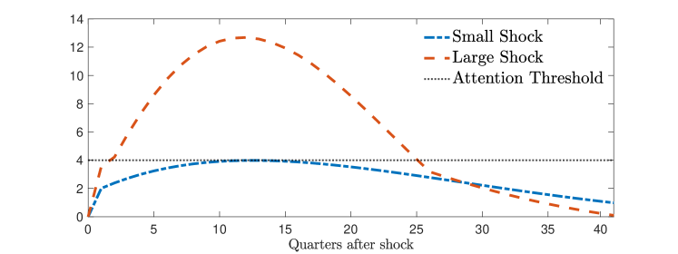
Figure 12: Inflation dynamics after a demand shock

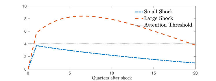
Figure 14: Inflation dynamics with $\gamma_{x,L}=0.25$ and $\gamma_{x,H}=0.1$

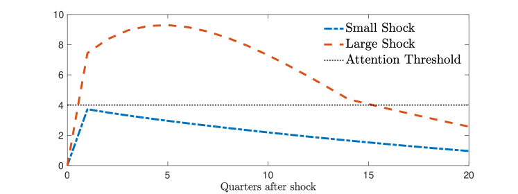
Figure 15: Inflation dynamics with current inflation as the threshold-defining variable

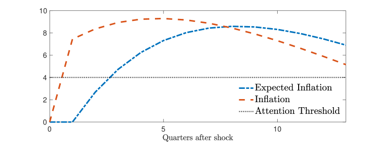
Figure 16: Forecast errors with current inflation as the threshold-defining variable

References

- Adam and Billi (2006) Adam, K. and R. M. Billi (2006): “Optimal monetary policy under commitment with a zero bound on nominal interest rates,” Journal of Money, Credit and Banking, 1877–1905.
- Adam and Padula (2011) Adam, K. and M. Padula (2011): “Inflation dynamics and subjective expectations in the United States,” Economic Inquiry, 49, 13–25.
- Afrouzi and Yang (2020) Afrouzi, H. and C. Yang (2020): “Dynamic inattention, the phillips curve, and forward guidance,” Tech. rep., Working Paper.
- Andre et al. (2022) Andre, P., C. Pizzinelli, C. Roth, and J. Wohlfart (2022): “Subjective models of the macroeconomy: Evidence from experts and representative samples,” The Review of Economic Studies, 89, 2958–2991.
- Angeletos et al. (2020) Angeletos, G.-M., Z. Huo, and K. Sastry (2020): “Imperfect expectations: Theory and evidence,” in NBER Macroeconomics Annual 2020, volume 35, University of Chicago Press.
- Angeletos and La’o (2010) Angeletos, G.-M. and J. La’o (2010): “Noisy business cycles,” NBER Macroeconomics Annual, 24, 319–378.
- Bayer et al. (2022) Bayer, C., B. Born, and R. Luetticke (2022): “Shocks, frictions, and inequality in US business cycles,” .
- Benati (2008) Benati, L. (2008): “Investigating inflation persistence across monetary regimes,” The Quarterly Journal of Economics, 123, 1005–1060.
- Benigno and Eggertsson (2023) Benigno, P. and G. B. Eggertsson (2023): “It’s baaack: The surge in inflation in the 2020s and the return of the non-linear phillips curve,” Working paper.
- Benigno and Paciello (2014) Benigno, P. and L. Paciello (2014): “Monetary policy, doubts and asset prices,” Journal of Monetary Economics, 64, 85–98.
- Bernanke and Blanchard (2023) Bernanke, B. and O. Blanchard (2023): “What caused the US pandemic-era inflation?” Hutchins Center Working Papers.
- Bhandari et al. (2019) Bhandari, A., J. Borovička, and P. Ho (2019): “Survey data and subjective beliefs in business cycle models,” .
- Bianchi and Melosi (2022) Bianchi, F. and L. Melosi (2022): “Inflation as a fiscal limit,” .
- Blanco et al. (2022) Blanco, A., P. Ottonello, and T. Ranosova (2022): “The Dynamics of Large Inflation Surges,” Working paper.
- Bracha and Tang (2023) Bracha, A. and J. Tang (2023): “Inflation levels and (in) attention,” Working Paper.
- Broer et al. (2021) Broer, T., A. Kohlhas, K. Mitman, and K. Schlafmann (2021): “Information and wealth heterogeneity in the macroeconomy,” Working paper.
- Candia et al. (2021) Candia, B., O. Coibion, and Y. Gorodnichenko (2021): “The Inflation Expectations of US Firms: Evidence from a New Survey,” Working paper.
- Candia et al. (2023) Candia, B., M. Weber, Y. Gorodnichenko, and O. Coibion (2023): “Perceived and Expected Rates of Inflation of US Firms,” 113, 52–55.
- Carlson and Parkin (1975) Carlson, J. A. and M. Parkin (1975): “Inflation expectations,” Economica, 42, 123–138.
- Carvalho et al. (2022) Carvalho, C., S. Eusepi, E. Moench, and B. Preston (2022): “Anchored inflation expectations,” American Economic Journal: Macroeconomics (forthcoming).
- Cavallo et al. (2017) Cavallo, A., G. Cruces, and R. Perez-Truglia (2017): “Inflation expectations, learning, and supermarket prices: Evidence from survey experiments,” American Economic Journal: Macroeconomics, 9, 1–35.
- Clarida et al. (1999) Clarida, R., J. Gali, and M. Gertler (1999): “The science of monetary policy: a new Keynesian perspective,” Journal of economic literature, 37, 1661–1707.
- Coibion and Gorodnichenko (2015) Coibion, O. and Y. Gorodnichenko (2015): “Is the Phillips curve alive and well after all? Inflation expectations and the missing disinflation,” American Economic Journal: Macroeconomics, 7, 197–232.
- Coibion et al. (2020) Coibion, O., Y. Gorodnichenko, E. S. I. Knotek, and R. Schoenle (2020): “Average Inflation Targeting and Household Expectations,” Journal of Political Economy (forthcoming).
- D’Acunto et al. (2023) D’Acunto, F., U. Malmendier, and M. Weber (2023): “What do the data tell us about inflation expectations?” in Handbook of economic expectations, Elsevier, 133–161.
- Di Giovanni et al. (2022) Di Giovanni, J., S. Kalemli Ozcan, A. Silva, and M. Yildirim (2022): “Global supply chain pressures, international trade, and inflation,” Working paper.
- D’Acunto et al. (2019) D’Acunto, F., D. Hoang, M. Paloviita, and M. Weber (2019): “Cognitive abilities and inflation expectations,” in AEA Papers and Proceedings, American Economic Association 2014 Broadway, Suite 305, Nashville, TN 37203, vol. 109, 562–566.
- D’Acunto et al. (2021) D’Acunto, F., U. Malmendier, and M. Weber (2021): “Gender roles produce divergent economic expectations,” Proceedings of the National Academy of Sciences, 118, e2008534118.
- Evans and Ramey (1995) Evans, G. W. and G. Ramey (1995): “Expectation calculation, hyperinflation and currency collapse,” The new macroeconomics: Imperfect markets and policy effectiveness, 307.
- Flynn and Sastry (2022) Flynn, J. P. and K. Sastry (2022): “Attention cycles,” Working Paper.
- Gagliardone and Gertler (2023) Gagliardone, L. and M. Gertler (2023): “Oil Prices, Monetary Policy and Inflation Surges,” Working paper.
- Galí (2015) Galí, J. (2015): Monetary policy, inflation, and the business cycle: an introduction to the new Keynesian framework and its applications, Princeton University Press.
- Gallegos (2023) Gallegos, J. E. (2023): “Inflation persistence, noisy information and the Phillips curve,” Working paper.
- Gáti (2022) Gáti, L. (2022): “Monetary Policy & Anchored Expectations An Endogenous Gain Learning Model,” Journal of Monetary Economics (forthcoming).
- Goldstein (2023) Goldstein, N. (2023): “Tracking inattention,” Journal of the European Economic Association, jvad022.
- Gonzalo and Pitarakis (2002) Gonzalo, J. and J.-Y. Pitarakis (2002): “Estimation and model selection based inference in single and multiple threshold models,” Journal of econometrics, 110, 319–352.
- Hansen (2011) Hansen, B. E. (2011): “Threshold autoregression in economics,” Statistics and its Interface, 4, 123–127.
- Hazell et al. (2022) Hazell, J., J. Herreno, E. Nakamura, and J. Steinsson (2022): “The slope of the Phillips Curve: evidence from US states,” The Quarterly Journal of Economics, 137, 1299–1344.
- Hilscher et al. (2022) Hilscher, J., A. Raviv, and R. Reis (2022): “How likely is an inflation disaster?” .
- Jørgensen and Lansing (2023) Jørgensen, P. L. and K. J. Lansing (2023): “Anchored inflation expectations and the slope of the phillips curve,” Working Paper.
- Kim and Binder (2023) Kim, G. and C. Binder (2023): “Learning-through-survey in inflation expectations,” American Economic Journal: Macroeconomics, 15, 254–278.
- Korenok et al. (2022) Korenok, O., D. Munro, and J. Chen (2022): “Inflation and attention thresholds,” Working paper.
- Kroner (2023) Kroner, N. (2023): “Inflation and Attention: Evidence from the Market Reaction to Macro Announcements,” Available at SSRN 4527424.
- Lamla and Lein (2014) Lamla, M. J. and S. M. Lein (2014): “The role of media for consumers’ inflation expectation formation,” Journal of Economic Behavior & Organization, 106, 62–77.
- Larsen et al. (2021) Larsen, V. H., L. A. Thorsrud, and J. Zhulanova (2021): “News-driven inflation expectations and information rigidities,” Journal of Monetary Economics, 117, 507–520.
- Macaulay (2022) Macaulay, A. (2022): “Shock transmission and the sources of heterogeneous expectations,” Working Paper.
- Maćkowiak et al. (2018) Maćkowiak, B., F. Matějka, and M. Wiederholt (2018): “Dynamic rational inattention: Analytical results,” Journal of Economic Theory, 176, 650–692.
- Maćkowiak et al. (2020) ——— (2020): “Rational Inattention: A Review,” .
- Mackowiak et al. (2023) Mackowiak, B., F. Matejka, and M. Wiederholt (2023): “Rational Inattention: A Review,” Journal of Economic Literature.
- Mackowiak and Wiederholt (2009) Mackowiak, B. and M. Wiederholt (2009): “Optimal sticky prices under rational inattention,” American Economic Review, 99, 769–803.
- Matějka and McKay (2015) Matějka, F. and A. McKay (2015): “Rational inattention to discrete choices: A new foundation for the multinomial logit model,” American Economic Review, 105, 272–98.
- McClure et al. (2022) McClure, E. M., O. Coibion, and Y. Gorodnichenko (2022): “The Macroeconomic Expectations of US Managers,” Working Paper.
- Meichtry (2022) Meichtry, P. (2022): “Sticky Information, Heterogeneity, and Aggregate Demand,” .
- Newey and West (1987) Newey, W. K. and K. D. West (1987): “A Simple, Positive Semi-Definite, Heteroskedasticity and Autocorrelation,” Econometrica, 55, 703–708.
- Nimark and Pitschner (2019) Nimark, K. P. and S. Pitschner (2019): “News media and delegated information choice,” Journal of Economic Theory, 181, 160–196.
- Nord (2022) Nord, L. (2022): “Who Cares about Inflation? Endogenous Expectation Formation of Heterogeneous Households,” Working paper.
- Paciello and Wiederholt (2014) Paciello, L. and M. Wiederholt (2014): “Exogenous information, endogenous information, and optimal monetary policy,” Review of Economic Studies, 81, 356–388.
- Pedemonte et al. (2023) Pedemonte, M., H. Toma, and E. Verdugo (2023): “Aggregate Implications of Heterogeneous Inflation Expectations: The Role of Individual Experience,” .
- Pfäuti (2023) Pfäuti, O. (2023): “Inflation–who cares? Monetary Policy in Times of Low Attention,” Working paper.
- Pfäuti and Seyrich (2023) Pfäuti, O. and F. Seyrich (2023): “A behavioral heterogeneous agent New Keynesian model,” Working paper.
- Pflueger (2023) Pflueger, C. (2023): “Back to the 1980s or not? The drivers of inflation and real risks in Treasury bonds,” Tech. rep., National Bureau of Economic Research.
- Reis (2022) Reis, R. (2022): “Losing the inflation anchor,” Brookings Papers on Economic Activity, 2021, 307–379.
- Rotemberg (1982) Rotemberg, J. J. (1982): “Sticky prices in the United States,” Journal of political economy, 90, 1187–1211.
- Roth et al. (2023) Roth, C., M. Wiederholt, and J. Wohlfart (2023): “The Effects of Monetary Policy: Theory with Measured Expectations,” Working paper.
- Schmidt et al. (2023) Schmidt, T., H. Müller, J. Rieger, T. Schmidt, and C. Jentsch (2023): “Inflation Perception and the Formation of Inflation Expectations,” Working paper.
- Sims (2003) Sims, C. A. (2003): “Implications of rational inattention,” Journal of monetary Economics, 50, 665–690.
- Sims (2010) ——— (2010): “Rational inattention and monetary economics,” in Handbook of monetary economics, Elsevier, vol. 3, 155–181.
- Vellekoop and Wiederholt (2019) Vellekoop, N. and M. Wiederholt (2019): “Inflation expectations and choices of households,” .
- Weber et al. (2022) Weber, M., F. D’Acunto, Y. Gorodnichenko, and O. Coibion (2022): “The subjective inflation expectations of households and firms: Measurement, determinants, and implications,” Journal of Economic Perspectives, 36, 157–184.
- Weber et al. (2023) Weber, M., S. Sheflin, T. Ropele, R. Lluberas, S. Frache, B. Meyer, S. Kumar, Y. Gorodnichenko, D. Georgarakos, O. Coibion, et al. (2023): “Tell Me Something I Don’t Already Know: Learning in Low and High-Inflation Settings,” .
- Woodford (2003) Woodford, M. (2003): Interest and Prices, Princeton University Press.