On High-Dimensional Asymptotic Properties of Model Averaging Estimators

Abstract

When multiple models are considered in regression problems, the model averaging method can be used to weigh and integrate the models. In the present study, we examined how the goodness-of-prediction of the estimator depends on the dimensionality of explanatory variables when using a generalization of the model averaging method in a linear model. We specifically considered the case of high-dimensional explanatory variables, with multiple linear models deployed for subsets of these variables. Consequently, we derived the optimal weights that yield the best predictions. we also observe that the double-descent phenomenon occurs in the model averaging estimator. Furthermore, we obtained theoretical results by adapting methods such as the random forest to linear regression models. Finally, we conducted a practical verification through numerical experiments.

1 Introduction

Owing to recent technological advances, tasks involving high-dimensional data have become increasingly ubiquitous. In a high-dimensional environment, estimators may exhibit unique behaviors not observed in lower-dimensional settings. For example, the spherical concentration (Hall et al., (2005)) and double descent (Advani et al., (2020); Belkin et al., (2019); Hastie et al., (2022); Bartlett et al., (2020)) have been reported as phenomena peculiar to high-dimensional data. These behaviors necessitate in-depth research into the properties of high-dimensional data.
In the present study, we estimated the explanatory coefficients $\beta$ to predict future target data $y$ using the following random linear regression model:

$$y_{i}=x_{i}^{\top}\beta+\epsilon_{i},\quad i=1,2,...,n$$ (1)

where each observation $x_{i}\in\mathbbm{R}^{p}$ and noise instance $\epsilon_{i}\in\mathbbm{R}$ is drawn i.i.d. from two independent distributions. Moreover, we assume that $\mathbbm{E}[x_{i}]=0$, $\mathbbm{E}[\epsilon_{i}]=0$, $\mathbbm{E}[x_{i}x_{i}^{\top}]=I$, and $\mathbbm{E}[\epsilon_{i}^{2}]=\sigma^{2}>0$ for $i=1,2,...,n$. To estimate the coefficients $\beta$ from $(x_{i},y_{i})$, we consider model averaging estimators obtained by constructing a new model through the integration of existing models, where each constituent model uses a min-norm least-squares estimator consisting of a distinct set of variables that may overlap with any of the other models’ sets. Specifically, we assume the preparation of $m$ candidate models, denoted as $M_{1},M_{2},...,M_{m}$, as follows:

$$M_{k}:\quad y=\sum_{i\in S_{i}}\beta_{i}x_{i}+\epsilon.$$ (2)

We estimate regression coefficients using the conventional min-norm least-squares method for each model, and obtain (4). After a list of candidate models is specified and their least-squares estimators are obtained, we predict the true value $\beta$ by using these estimators as follows:

$$\hat{y}=\sum_{i=1}^{m}w_{i}\hat{\beta}_{S_{i}}^{\top}x_{0,S_{i}},$$ (3)

where $w\in\mathbbm{R}^{m}$ is the weight vector with $\sum_{i=1}^{m}w_{i}=1$, each $S_{i}$ is a subset of the features (e.g., $S_{i}=\{1,4,5,7,...,p-1,p\}$), $x_{0}$ is a given future datum, $x_{0,S}$ is the subvector of $x_{0}$ that contains features whose indices are in $S$, and $\hat{\beta}_{S_{i},k}$ is the $k$-th entry of the min-norm least squares estimator $\hat{\beta}_{S}$ estimated using the variables represented by $x_{0,S}$. In other words,

$$\hat{\beta}_{S}=X_{S}^{+}y,$$ (4)

where $X_{S}$ denotes the $n\times|S|$ submatrix from which the columns comprising $S$ are taken. Here, $A^{+}$ denotes the Moore-Penrose inverse matrix of $A$. This predictor (3) is equivalent to estimating $\beta$ using the model averaging estimator $\hat{\beta}_{w}$, where the $k$-th entry $\hat{\beta}_{w,k}$ is expressed as

$$\hat{\beta}_{w,k}=\sum_{i=1}^{m}w_{i}\mathbbm{1}_{\{k\in S_{i}\}}\hat{\beta}_{S_{i},k},$$ (5)

for $k\in\mathbbm{N}$.

The selection of candidate models varies with respect to context. For several examples of candidate models, please refer to Hansen, (2007); Hansen and Racine, (2012); Ando and Li, (2014) and the references therein.

In general, we consider the model averaging estimator $\hat{\beta}_{w,k}$, whose $k$th entry is expressed as

$$\hat{\beta}_{w,k}=\sum_{i=1}^{m}w_{i}\mathbbm{1}_{\{k\in S_{i}\}}\hat{\beta}_{S_{i},k}^{T_{i}},$$ (6)

for $k\in\mathbbm{N}$, where $w\in\mathbbm{R}^{m}$ is the weight vector with $\sum_{i=1}^{m}w_{i}=1$, each $S_{i}$ is a subset of the features (e.g., $S_{i}=\{1,4,5,7,...,p-1,p\}$), each $T_{i}$ is a subset of the samples (e.g. $T_{i}=\{1,2,5,6,...,n-2,n\}$), and $\hat{\beta}_{S}^{T}$ is the min-norm least-squares estimator obtained by using $T_{i}$ and $S_{i}$, i.e.,

$$\hat{\beta}_{S}^{T}=X_{S}^{T+}y_{T}.$$ (7)

Here, $X_{S}^{T}$ denotes the $|T|\times|S|$ submatrix from which the rows comprising $T$ and columns comprising $S$ are taken, and $y_{T}$ denotes the subvector of $y$ containing features whose indices are in $T$. This estimator is equivalent to predicting the target value $y_{0}=\beta^{\top}x_{0}$ using

$$\hat{y}=\sum_{i=1}^{m}w_{i}\hat{\beta}^{T_{i}\top}_{S_{i}}x_{0,S_{i}},$$ (8)

where $x_{0}$ is a given future datum and $x_{0,S}$ is the subvector of $x_{0}$ containing features whose indices are in $S$. It is clear that the above estimators accommodate ordinal model-averaging estimators.

This kind of estimators may emerge in the context of distributed learning. For example, let us consider the case where different feature sets are used at different locations to independently construct an estimator for the same target variable, and only the information from that estimator can be used. This study may be of some help as an answer to what weights should be used to aggregate these estimators. Also, if $T$’s are chosen uniformly at random, this would be like bagging, which are also analyzed in LeJeune et al., (2020); Patil et al., (2022).

We analyzed this estimator under both the underparametrized $n>p$ and the overparametrized $n<p$ regime via random matrix theory (RMT), and derived optimal weight. For the estimator $\hat{\beta}$, we express our result in terms of the out-of-sample risk:

$$R_{X}(\hat{\beta})\coloneqq\mathbbm{E}\left[(\hat{y}_{0}-\beta^{\top}x_{0})^{2}\mid X\right]=\mathbbm{E}\left[\|\hat{\beta}-\beta\|^{2}\mid X\right],$$

where $\hat{y}_{0}=\hat{\beta}^{\top}x_{0}$ and the expectation is taken as an independent random test sample $x_{0}$ from an equivalent distribution to that of the training data. Because we assume that $\mathbbm{E}[x_{i}x_{i}^{\top}]=I$ for $i=0,1,2,...,n$, the out-of-sample risk is reduced to an ordinal-squared risk, which can be regarded as a predictive risk. We also observe that the double descent phenomenon occurs as a byproduct under certain conditions when using this estimator. Although the above assumptions are simple, this model reveals new insights into model averaging estimators. Furthermore, if, for example, the data $x_{i}\quad(i=1,...,n)$ follow a normal distribution $N(0,\Sigma)$, then under the perspective of predicting the target variable $y$, the linear model

$$y=X\beta+\epsilon,$$

is equivalent to the following linear model:

$$y=Z\Sigma^{\frac{1}{2}}\beta+\epsilon,$$

where $Z=(z_{1},...,z_{n})^{\top}$ and $z_{i}\sim N(0,\mathrm{I}),\quad(i=1,...,n)$. Therefore, the analysis conducted in this study may be applicable if the data matrix is whitened.

1.1 Contribution

Our contributions can be summarized as follows:

Precise analysis of model averaging estimators. Using RMT, we calculated and characterized the goodness-of-prediction of the model averaging estimator in a linear model under the assumption that isotropic samples have been obtained. Our results also reveal that the double descent phenomenon occurs when using such an estimator. In addition, we derived the high-dimensional asymptotic behavior of each model when the samples and features were selected randomly.

Optimal weights. A model averaging estimator consists of a weight vector and several min-norm least-squares estimators. The weight vector can be optimized to achieve the prediction of true values. As we derived a precise theoretical curve for the predictive risk of this estimator, we obtained the optimal weight vector according to certain conditions assumed in this study.

The first contribution above can be regarded as the extension of Theorem 3.5 in LeJeune et al., (2020), where precise asymptotic risk was obtained under the condition that the dimensionality of data does not exceed the number of samples. In contrast, we were able to deduce high-dimensional behavior of the model averaging estimator even when the dimensionality of data exceeded the number of samples. In addition, this study partially extends the result of Theorem 1 in Hastie et al., (2022), which investigated the double descent phenomenon of the min-norm least-squares estimators of linear regression. Whereas the study in question considered a single model estimator, we examined the integration of multiple model estimators.

1.2 Framework of high-dimensional asymptotics

This section presents relevant notations and assumptions in terms of high-dimensional asymptotics.

Unlike previous studies Hansen, (2007); Hansen and Racine, (2012); Ando and Li, (2014), We use RMT to analyze the precise predictive risk of estimators. RMT enables us to describe the behavior of the eigenvalues of large matrices (see, e.g. Bai and Silverstein, (2010)). These results are typically stated in terms of the spectral distribution $F_{A}(x)\coloneqq p^{-1}\sum^{p}_{k=1}\mathbbm{1}_{\{\lambda_{k}(A)\leq x\}}$, which is the cumulative distribution function of the eigenvalues $\lambda_{k}(A),k=1,...,p$ of a symmetric matrix $A$. The following high-dimensional asymptotic model is assumed for all theorems and corollaries.

Assumption 1 (High-Dimensional Asymptotics).

The following conditions hold:

• Data $X_{n}\in\mathbb{R}^{n\times p}$ are generated with i.i.d. entries satisfying $\mathbbm{E}\left[X_{n,ij}\right]=0$, $\mathrm{Var}\left[X_{n,ij}\right]=1$ $\mathbbm{E}\left[|X_{n,ij}|^{12+\omega}\right]<\infty$ for an $\omega>0$.

• The sample size $n\to\infty$ and dimension $p\to\infty$ as well, whereas the aspect ratio $p/n\to\gamma>0$.

• The dimensions of candidate models $|S^{n}_{i}|\to\infty$, $|S^{n}_{i}\cap S^{n}_{j}|\to\infty$ as $n\to\infty$; conversely, $|S^{n}_{i}|/n\to\gamma_{i}>0$ and $|S^{n}_{i}\cap S^{n}_{j}|/n\to\gamma_{ij}>0$ for any $i,j$.

• The samples used in the candidate models $|T^{n}_{i}|\to\infty$ as $n\to\infty$; conversely, $|T^{n}_{i}|/n\to\eta_{i}>0$ and $|T^{n}_{i}\cap T^{n}_{j}|/n\to\eta_{ij}>0$ for any $i$.

• The weight vector $w_{n}\in\mathbbm{R}^{m}$ satisfies $\sum_{i=1}^{m}w_{n,i}=1$ and converges to a weight vector $w\in\mathbbm{R}^{m}$ as $n\to\infty$, $p\to\infty$ and $p/n\to\gamma$.

Similar conditions have been assumed in Dobriban and Wager, (2018), Hastie et al., (2022), Wu and Xu, (2020) and Richards et al., (2021). Unlike in previous studies (Bai and Silverstein, (1998), Bai and Silverstein, (2010), Fujikoshi, (2022), Dobriban and Wager, (2018), Hastie et al., (2022)), Assumption 1 is more restrictive in that it includes the condition $\mathbbm{E}\left[X_{n,ij}^{12+\omega}\right]<\infty$ for theoretical purposes. Specifically, this condition is necessary when applying the trace lemma to obtain the result of Lemma A.6. However, many distributions, such as the Laplace and Gaussian distributions, satisfy these conditions. Note that the risk of the model averaging estimator does not depend only on the eigenvalues, and classical RMT methods cannot be applied under the present settings. Hence, we must prove certain RMT results that are specified in the present assumptions.

We also assume the following throughout this study:

Assumption 2 (Deterministic Coefficients).

The regression coefficients $\beta_{n}\in\mathbbm{R}^{p}$ satisfy $\|\beta_{n}\|^{2}=r^{2}$ for $r>0$.

To simplify the notation, we omit the subscript n by denoting $X_{n}$ as $X$, $S^{n}_{i}$ as $S_{i}$, $T^{n}_{i}$ as $T_{i}$, and $\beta_{n}$ as $\beta$.

1.3 Related works

Model averaging estimator for linear regression. Model averaging estimators have been the subject of extensive research. For example, Akaike, (1978, 1979); Hansen, (2007); Hansen and Racine, (2012); Ando and Li, (2014) estimated target variables by weighting and adding the estimators in a linear model, with weights determined using various model selection criteria. Akaike, (1978, 1979) considered the Akaike information criterion (AIC), Hansen, (2007) used the $C_{p}$ criterion (Mallows, (2000)), Hansen and Racine, (2012) employed the Jackknife method, and Ando and Li, (2014) considered using cross-validation to determine the weight vector. Each of these studies demonstrated that under the appropriate conditions, the weights derived using their respective selection methods were optimal for estimation. In particular, Ando and Li, (2014) considered high-dimensional models and demonstrated their optimality under an unusual range of weighting definitions. However, all of these studies assumed the dimensionality of each candidate model to be less than the number of samples. Conversely, we examined behavior under a dimensionality exceeding the number of samples.

Several model averaging methods: bagging and distributed learning. In the present study, we categorized the data in terms of both the sample and feature indices. Such an averaging approach was also considered in LeJeune et al., (2020), wherein samples and features were extracted randomly. However, we also considered the case of non-random extraction. Patil et al., (2022) obtained results for bagging and sub-bagging, where only samples were extracted randomly. Specifically, they examined the high-dimensional asymptotic behaviors of ridge and ridgeless estimators with respect to bagging and sub-bagging. In addition, Dobriban and Sheng, (2021, 2020) studied model integration methods under non-random sample partitioning in the context of distributed learning.

High-dimensional analysis via random matrix theory. In the present study, we employed RMT Bai and Silverstein, (2010) to establish theoretical results. Previously, RMT has been applied for various statistical tasks. For example, Ledoit and Wolf, (2012, 2020) used RMT to estimate covariance matrices. Hastie et al., (2022); Dobriban and Wager, (2018); Dobriban and Sheng, (2020, 2021); Patil et al., (2022) considered the properties of ridge and ridgeless estimators, as well as linear model integration estimators, in an RMT framework. Fujikoshi, (2022) used RMT to examine properties related to the consistency of model selection, such as the AIC Akaike, (1974) and Bayesian Information Criterion (BIC, Schwarz, (1978)), for multivariate linear regression problems. Hu and Li, (2022) developed a method for estimating the signal-to-noise ratios (SNRs) of linear models using RMT. All aforementioned studies examined estimator behaviors and model selection criteria with high-dimensional data, demonstrating the powerful analytical performance of RMT under a high-dimensional setting.

Double decent phenomenon in linear models. The double descent phenomenon has been the subject of intense research, e.g. Hastie et al., (2022); Derezinski et al., (2020); Patil et al., (2022). In machine learning and especially deep learning, data are often used to train models with large numbers of parameters. Conventional wisdom states that an excessive number of training parameters may lead to overfitting, deteriorating a model’s predictive performance. However, when the number of parameters exceeds a certain threshold, the opposite has been observed to occur, with predictive performance improving. This is known as the double descent phenomenon because the risk of forecasting exhibits an increase followed by a decrease (Advani et al., (2020); Belkin et al., (2019)). In a linear model, increasing the number of parameters increases dimensionality. Hastie et al., (2022) demonstrated that when the number of samples falls below the dimensionality, predictive performance increases. Derezinski et al., (2020) also demonstrated the double decent phenomenon in a different framework. Patil et al., (2022) examined the behavior of bagged ridge and ridgeless estimators in higher dimensions, with the ensemble estimator also exhibiting double descent.

1.4 Outline

The remainder of this paper is organized as follows. Section 2 presents our primary theoretical results. A verification of these results through simulation studies is given in Section 3. In Section 4, we summarize our results and discuss future directions of research. Proofs of the theoretical results are provided in the Appendix.

2 Main results

The following subsections present the main results of this study. Proofs of the theorems used in this section are provided in the Appendix.

2.1 Out-of-sample risk of model averaging estimators

We begin by examining the predictive behavior of model-averaging estimators when each candidate model contains the true model. As described in the first section, we estimate $\beta$ using a model averaging estimator:

$$\hat{\beta}_{w,k}=\sum_{i=1}^{m}w_{n,i}\mathbbm{1}_{\{i\in S_{i}\}}\hat{\beta}^{T_{i}}_{S_{i},k},$$

where $w\in\mathbbm{R}^{m}$ is the weight vector with $\sum_{i=1}^{m}w_{i}=1$, $S_{i}$ is a subset of features, and $T_{i}$ is a subset of samples.

We derive the following theorem for out-of-sample risk:

Theorem 2.1.

Suppose that the assumption 1 and 2 holds and each candidate model contains a true model. Then, almost surely,

$$R_{X}(\hat{\beta}_{w})\to w^{\top}Hw,$$ (9)

where $H=(h_{ij})$ is a positive definite matrix defined as follows:

$$h_{ii}=\begin{cases}\sigma^{2}\frac{\gamma_{i}}{\eta_{i}-\gamma_{i}}&\gamma_{i}<\eta_{i}\\ \left(1-\frac{\eta_{i}}{\gamma_{i}}\right)r^{2}+\frac{\eta_{i}}{\gamma_{i}-\eta_{i}}\sigma^{2}&\gamma_{i}>\eta_{i}\end{cases}$$ (10)

$$h_{ij}=\begin{cases}\frac{\eta_{ij}\gamma_{ij}}{\eta_{i}\eta_{j}-\eta_{ij}\gamma_{ij}}\sigma^{2}&\gamma_{i}<\eta_{i},\gamma_{j}<\eta_{j}\\ \frac{\eta_{ij}\gamma_{ij}}{\eta_{i}\gamma_{j}-\eta_{ij}\gamma_{ij}}\sigma^{2}&\gamma_{i}<\eta_{i},\eta_{j}<\gamma_{j}\\ \frac{\eta_{ij}\gamma_{ij}}{\eta_{j}\gamma_{i}-\eta_{ij}\gamma_{ij}}\sigma^{2}&\gamma_{j}<\eta_{j},\eta_{i}<\gamma_{i}\\ \frac{(\gamma_{i}-\eta_{i})(\gamma_{j}-\eta_{j})}{\gamma_{i}\gamma_{j}-\eta_{ij}\gamma_{ij}}r^{2}+\frac{\eta_{ij}\gamma_{ij}}{\gamma_{i}\gamma_{j}-\eta_{ij}\gamma_{ij}}\sigma^{2}&\eta_{i}<\gamma_{i},\eta_{j}<\gamma_{j}\end{cases}$$ (11)

for $i,j=1,2,...,m,i\neq j$.

Proof.

The proof is provided in the Appendix. ∎

From the above Theorem, we can immediately obtain the following result t by employing Lagrange multiplier method.

Corollary 2.2.

Define signal-to-noise ratio $\mathrm{SNR}=r^{2}/\sigma^{2}$. If we can estimate $\mathrm{SNR}$ by a consistent estimator $\hat{\Gamma}$, then

$$w_{\mathrm{opt}}=\frac{1}{\mathbbm{1}^{\top}\hat{H}^{-1}\mathbbm{1}}\hat{H}^{-1}\mathbbm{1}\to\mathrm{argmin}_{w}w^{\top}Hw,$$

where $\mathbbm{1}=(1,1,\cdots,1)^{\top}$ and $\hat{H}=(\hat{h}_{ij})$ is defined as follows:

$$\hat{h}_{ii}=\begin{cases}\frac{\gamma_{i}}{\eta_{i}-\gamma_{i}}&\gamma_{i}<\eta_{i}\\ \left(1-\frac{\eta_{i}}{\gamma_{i}}\right)\hat{\Gamma}+\frac{\eta_{i}}{\gamma_{i}-\eta_{i}}&\eta_{i}<\gamma_{i}\end{cases}$$

$$\tilde{h}_{ij}^{1}=\begin{cases}\frac{\eta_{ij}\gamma_{ij}}{\eta_{i}\eta_{j}-\eta_{ij}\gamma_{ij}}&\gamma_{i}<\eta_{i},\gamma_{j}<\eta_{j}\\ \frac{\eta_{ij}\gamma_{ij}}{\eta_{i}\gamma_{j}-\eta_{ij}\gamma_{ij}}&\gamma_{i}<\eta_{i},\eta_{j}<\gamma_{j}\\ \frac{\eta_{ij}\gamma_{ij}}{\eta_{j}\gamma_{i}-\eta_{ij}\gamma_{ij}}&\gamma_{j}<\eta_{j},\eta_{i}<\gamma_{i}\\ \frac{(\gamma_{i}-\eta_{i})(\gamma_{j}-\eta_{j})}{\gamma_{i}\gamma_{j}-\eta_{ij}\gamma_{ij}}\hat{\Gamma}+\frac{\eta_{ij}\gamma_{ij}}{\gamma_{i}\gamma_{j}-\eta_{ij}\gamma_{ij}}&\eta_{i}<\gamma_{i},\eta_{j}<\gamma_{j}\end{cases}$$

for $i,j=1,2,...,m,i\neq j$.

The problem of estimating $\mathrm{SNR}$ has been studied extensively ( refer to Jiang and Nguyen, (2007); Dicker, (2014); Jiang et al., (2016); Janson et al., (2017) for examples). More recently, have been derived under high-dimensional asymptotics using RMT (Hu and Li, (2022)). For practical purposes, it is also necessary to estimate $\gamma_{i}$ and $\eta_{i}$, which can be estimated in $|S_{i}|/n$ and $|T_{i}|/n$, respectively. In the following subsection, we consider more realistic situations wherein some models are misspecified.

2.2 Out-of-sample risk of model averaging estimators: misspecified case

In this section, we consider the case where some candidate models do not include the entire true model. Letting $\beta$ denote the regression coefficient of the true model and assuming $\|\beta_{S_{i}}\|^{2}=r^{2}\kappa_{i}$ and $\|\beta_{(S_{i}\cap S_{j})}\|^{2}=r^{2}\kappa_{ij}$, where $\kappa_{i}\in(0,1),\kappa_{ij}\in(0,1)$ for $i,j=1,...,m,i\neq j$, we obtain the following result:

Theorem 2.3.

Suppose that assumption 1, 2 hold. Then, almost surely,

$$\mathbbm{E}\left[R_{X}(\hat{\beta}_{w})\right]\to w^{\top}H_{\mathrm{mis}}w,$$ (12)

where the expectation is taken over all $X$ and $H_{\mathrm{mis}}=(h_{\mathrm{mis},ij})$ is a positive definite matrix defined as follows:

$$h_{\mathrm{mis},ii}=\begin{cases}\frac{\eta_{i}}{\eta_{i}-\gamma_{i}}r^{2}(1-\kappa_{i})+\frac{\gamma_{i}}{\eta_{i}-\gamma_{i}}\sigma^{2}&\gamma_{i}<\eta_{i}\\ \frac{\gamma_{i}}{\gamma_{i}-\eta_{i}}r^{2}(1-\kappa_{i})+\left(1-\frac{\eta_{i}}{\gamma_{i}}\right)r^{2}\kappa_{i}+\frac{\eta_{i}}{\gamma_{i}-\eta_{i}}\sigma^{2}&\eta_{i}<\gamma_{i}\end{cases}$$

$$h_{\mathrm{mis},ij}=\begin{cases}\frac{\eta_{i}\eta_{j}}{\eta_{i}\eta_{j}-\eta_{ij}\gamma_{ij}}r^{2}(1-\kappa_{i}-\kappa_{j}+\kappa_{ij})+\frac{\eta_{ij}\gamma_{ij}}{\eta_{i}\eta_{j}-\eta_{ij}\gamma_{ij}}\sigma^{2}&\gamma_{i}<\eta_{i},\gamma_{j}<\eta_{j}\\ \frac{\eta_{i}\gamma_{j}}{\eta_{i}\gamma_{j}-\eta_{ij}\gamma_{ij}}r^{2}(1-\kappa_{i}-\kappa_{j}+\kappa_{ij})+\frac{\eta_{i}(\gamma_{j}-\eta_{j})}{(\eta_{i}\gamma_{j}-\eta_{ij}\gamma_{ij})}r^{2}(\kappa_{j}-\kappa_{ij})+\frac{\eta_{ij}\gamma_{ij}}{\eta_{i}\gamma_{j}-\eta_{ij}\gamma_{ij}}\sigma^{2}&\gamma_{i}<\eta_{i},\eta_{j}<\gamma_{j}\\ \frac{\eta_{j}\gamma_{i}}{\eta_{j}\gamma_{i}-\eta_{ij}\gamma_{ij}}r^{2}(1-\kappa_{i}-\kappa_{j}+\kappa_{ij})+\frac{\eta_{j}(\gamma_{i}-\eta_{i})}{\eta_{j}\gamma_{i}-\eta_{ij}\gamma_{ij}}r^{2}(\kappa_{i}-\kappa_{ij})+\frac{\eta_{ij}\gamma_{ij}}{\eta_{i}\gamma_{i}-\eta_{ij}\gamma_{ij}}\sigma^{2}&\gamma_{j}<\eta_{i},\eta_{j}<\gamma_{i}\\ \frac{\gamma_{i}\gamma_{j}}{\gamma_{i}\gamma_{j}-\eta_{ij}\gamma_{ij}}r^{2}(1-\kappa_{i}-\kappa_{j}+\kappa_{ij})+\frac{\gamma_{i}(\gamma_{j}-\eta_{j})}{\gamma_{i}\gamma_{j}-\eta_{ij}\gamma_{ij}}r^{2}(\kappa_{j}-\kappa_{ij})+\frac{\gamma_{j}(\gamma_{i}-\eta_{i})}{\gamma_{i}\gamma_{j}-\eta_{ij}\gamma_{ij}}r^{2}(\kappa_{i}-\kappa_{ij})\\ \quad\quad\quad+\frac{(\gamma_{i}-\eta_{i})(\gamma_{j}-\eta_{j})}{\gamma_{i}\gamma_{j}-\eta_{ij}\gamma_{ij}}r^{2}\kappa_{ij}+\frac{\eta_{ij}\gamma_{ij}}{\gamma_{i}\gamma_{j}-\eta_{ij}\gamma_{ij}}\sigma^{2}&\eta_{i}<\gamma_{i},\eta_{j}<\gamma_{j}\end{cases}$$ (13)

for $i,j=1,2,...,m,i\neq j$.

Proof.

The proof is provided in the Appendix. ∎

As before, this theorem can be combined with Lagrange’s undetermined multiplier method to deduce the following result:

Corollary 2.4.

Define signal-to-noise ratio $\mathrm{SNR}=r^{2}/\sigma^{2}$,$\mathrm{SNR}_{i}=r^{2}\kappa_{i}/\sigma^{2}$ and $\mathrm{SNR}_{ij}=r^{2}\kappa_{ij}/\sigma^{2}$ for $i,j=1,2,...,m,i\neq j$. If we can estimate $\mathrm{SNR}=r^{2}/\sigma^{2},\mathrm{SNR}_{i}=r^{2}\kappa_{i}/\sigma^{2},\mathrm{SNR}_{ij}=r^{2}\kappa_{ij}/\sigma^{2}$ by consistent estimators $\hat{\Gamma},\hat{\Gamma}_{i},\hat{\Gamma}_{ij}$, respectively, for $i,j=1,2,...,m,i\neq j$, then

$$w_{\mathrm{opt}}=\frac{1}{\mathbbm{1}^{\top}\hat{H}_{\mathrm{mis}}^{-1}\mathbbm{1}}\hat{H}_{\mathrm{mis}}^{-1}\mathbbm{1}\to\mathrm{argmin}_{w}w^{\top}H_{\mathrm{mis}}w,$$

where $\mathbbm{1}=(1,1,\cdots,1)^{\top}$ and $\hat{H}_{\mathrm{mis}}=(\hat{h}_{\mathrm{mis},ij})$ is defined as follows:

$$\hat{h}_{\mathrm{mis},ii}=\begin{cases}\frac{\eta_{i}}{\eta_{i}-\gamma_{i}}(\hat{\Gamma}-\hat{\Gamma}_{i})+\frac{\gamma_{i}}{\eta_{i}-\gamma_{i}}&\gamma_{i}<\eta_{i}\\ \frac{\gamma_{i}}{\gamma_{i}-\eta_{i}}(\hat{\Gamma}-\hat{\Gamma}_{i})+\left(1-\frac{\eta_{i}}{\gamma_{i}}\right)\hat{\Gamma}_{i}+\frac{\eta_{i}}{\gamma_{i}-\eta_{i}}&\eta_{i}<\gamma_{i}\end{cases}$$

$$\hat{h}_{\mathrm{mis},ij}=\begin{cases}\frac{\eta_{i}\eta_{j}}{\eta_{i}\eta_{j}-\eta_{ij}\gamma_{ij}}(\hat{\Gamma}-\hat{\Gamma}_{i}-\hat{\Gamma}_{j}+\hat{\Gamma}_{ij})+\frac{\eta_{ij}\gamma_{ij}}{\eta_{i}\eta_{j}-\eta_{ij}\gamma_{ij}}&\gamma_{i}<\eta_{i},\gamma_{j}<\eta_{j}\\ \frac{\eta_{i}\gamma_{j}}{\eta_{i}\gamma_{j}-\eta_{ij}\gamma_{ij}}(\hat{\Gamma}-\hat{\Gamma}_{i}-\hat{\Gamma}_{j}+\hat{\Gamma}_{ij})+\frac{\eta_{i}(\gamma_{j}-\eta_{j})}{(\eta_{i}\gamma_{j}-\eta_{ij}\gamma_{ij}})(\hat{\Gamma}_{j}-\hat{\Gamma}_{ij})+\frac{\eta_{ij}\gamma_{ij}}{\eta_{i}\gamma_{j}-\eta_{ij}\gamma_{ij}}&\gamma_{i}<\eta_{i},\eta_{j}<\gamma_{j}\\ \frac{\eta_{j}\gamma_{i}}{\eta_{j}\gamma_{i}-\eta_{ij}\gamma_{ij}}(\hat{\Gamma}-\hat{\Gamma}_{i}-\hat{\Gamma}_{j}+\hat{\Gamma}_{ij})+\frac{\eta_{j}(\gamma_{i}-\eta_{i})}{\eta_{j}\gamma_{i}-\eta_{ij}\gamma_{ij}}(\hat{\Gamma}_{i}-\hat{\Gamma}_{ij})+\frac{\eta_{ij}\gamma_{ij}}{\eta_{i}\gamma_{i}-\eta_{ij}\gamma_{ij}}&\gamma_{j}<\eta_{i},\eta_{j}<\gamma_{i}\\ \frac{\gamma_{i}\gamma_{j}}{\gamma_{i}\gamma_{j}-\eta_{ij}\gamma_{ij}}(\hat{\Gamma}-\hat{\Gamma}_{i}-\hat{\Gamma}_{j}+\hat{\Gamma}_{ij})+\frac{\gamma_{i}(\gamma_{j}-\eta_{j})}{\gamma_{i}\gamma_{j}-\eta_{ij}\gamma_{ij}}(\hat{\Gamma}_{j}-\hat{\Gamma}_{ij})+\frac{\gamma_{i}(\gamma_{j}-\eta_{j})}{\gamma_{i}\gamma_{j}-\eta_{ij}\gamma_{ij}}(\hat{\Gamma}_{i}-\hat{\Gamma}_{ij})\\ \quad\quad\quad+\frac{(\gamma_{i}-\eta_{i})(\gamma_{j}-\eta_{j})}{\gamma_{i}\gamma_{j}-\eta_{ij}\gamma_{ij}}\hat{\Gamma}_{ij}+\frac{\eta_{ij}\gamma_{ij}}{\gamma_{i}\gamma_{j}-\eta_{ij}\gamma_{ij}}&\eta_{i}<\gamma_{i},\eta_{j}<\gamma_{j}\end{cases}$$

for $i,j=1,2,...,m,i\neq j$.

It is easy to find consistent estimators of $\hat{\Gamma}_{i}$’s using a technique similar to that in Dicker, (2014), where the noise variance $\sigma^{2}$ and overall signal strength $r^{2}$ were estimated using

$$\hat{\sigma}^{2}=\frac{p+n+1}{n(n+1)}\|y\|^{2}-\frac{1}{n(n+1)}\|X^{\top}y\|^{2},\quad\hat{r}^{2}=-\frac{p}{n(n+1)}\|y\|^{2}+\frac{1}{n(n+1)}\|X^{\top}y\|^{2},$$ (14)

respectively. If a model is specified and each element of $X$ follows an i.i.d. normal distribution with mean $0$ and variance $1$, then the above estimators (14) are unbiased. Hence, we can estimate $\mathrm{SNR}$ using $\hat{r}^{2}/\hat{\sigma}^{2}$. These estimators can be determined using the following identities:

$$\mathbbm{E}\left[\frac{1}{n}\|y\|^{2}\right]=r^{2}+\sigma^{2},\quad\mathbbm{E}\left[\frac{1}{n^{2}}\|X^{\top}y\|^{2}\right]=\frac{p+n+1}{n}r^{2}+\frac{p}{n}\sigma^{2}.$$ (15)

Under the same assumption as above (i.e., the model is specified and each element of $X$ follows an i.i.d. normal distribution with mean $0$ and variance $1$), we can also obtain the following result given an $n\times p_{1}$ submatrix $X_{1}$ of matrix $X=(X_{1},X_{2})$:

$$\mathbbm{E}\left[\frac{1}{n^{2}}\|X_{1}^{\top}y\|^{2}\right] =\frac{n+1}{n}r_{1}^{2}+\frac{p_{1}}{n}(r^{2}+\sigma^{2})$$

$$=\frac{n+1}{n}r_{1}^{2}+\frac{p_{1}}{n}\mathbbm{E}\left[\frac{1}{n}\|y\|^{2}\right]$$ (16)

where $r_{1}^{2}$ is the signal strength of subvector $\beta_{1}$ of $\beta$ corresponding to $X_{1}$. Therefore, we can estimate $r_{1}^{2}/\sigma^{2}$ using

$$\frac{1}{n(n+1)\hat{\sigma}^{2}}\|X_{1}^{\top}y\|^{2}-\frac{p_{1}}{n(n+1)\hat{\sigma}^{2}}\|y\|^{2}.$$ (17)

We can easily verify the consistency of this estimator under the assumption 1.

2.3 Out-of-sample risk of model averaging estimators: linear ensemble case

In this section, we consider the case in which candidate models are chosen uniformly and randomly. Specifically, we define the following assumptions:

Assumption 3.

We assume the following hold:

• $\mathrm{Pr}(j\in S_{i})=|S_{i}|/p$ for all j=1,…,p.

• $\mathrm{Pr}(j\in T_{i})=|T_{i}|/n$ for all j=1,…,n.

• $|S_{i}|/p\to\alpha$ as $n,p\to\infty$ for any $i$.

• $|T_{i}|/n\to\eta$ as $n,p\to\infty$ for any $i$.

Furthermore, we consider the case where $w_{i}=1/m$ for all $i=1,...,m$. This estimator can be regarded as a linear version of the random forest. The following lemma is helpful in obtaining the asymptotic behavior of the estimator $\hat{\beta}_{\mathrm{ens}}$:

Lemma 2.5.

For any Lipschitz continuous function $f$,

$$\mathbbm{E}\left[f(|S_{i}\cap S_{j}|/p)\right]\to f(\alpha^{2}).$$ (18)

$$\mathbbm{E}\left[f(|T_{i}\cap T_{j}|/n)\right]\to f(\eta^{2}).$$ (19)

Proof.

Because $\mathbbm{E}\left[\left.\frac{|S_{i}\cap S_{j}|}{p}\right||S_{i}|,|S_{j}|\right]=\frac{|S_{i}||S_{j}|}{p^{2}}\to\alpha^{2}$, we only have to prove the following:

$$\mathbbm{E}\left[\left.\left|\frac{|S_{i}\cap S_{j}|}{p}-\mathbbm{E}\left[\left.\frac{|S_{i}\cap S_{j}|}{p}\right||S_{i}|,|S_{j}|\right]\right|\right||S_{i}|,|S_{j}|\right]\to 0.$$ (20)

This can be easily observed in

$$\mathrm{Var}\left(\left.\frac{|S_{i}\cap S_{j}|}{p}\right||S_{i}|,|S_{j}|\right)=O\left(\frac{1}{p}\right).$$

The latter part of the claim can be demonstrated in a similar manner, thereby completing the Proof. ∎

From the above Lemma, we obtain the following result together with Theorem 2.3 and its proof.

Theorem 2.6.

Suppose that assumption 1, 2 and 3 hold. Then, almost surely,

$$\mathbbm{E}\left[R_{X}(\hat{\beta}_{\mathrm{ens}})\right]\to\frac{1}{m}D+\frac{m-1}{m}N,$$ (21)

where the expectation is taken over $X$, $S$’s and $T$’s; and $D$ and $N$ are defined as,

$$D=\begin{cases}\frac{\eta(1-\alpha)}{\eta-\gamma\alpha}r^{2}+\sigma^{2}\frac{\gamma\alpha}{\eta-\gamma\alpha}&\gamma\alpha<\eta,\\ \frac{\gamma\alpha(1-\alpha)}{\gamma\alpha-\eta}r^{2}+\left(1-\frac{\eta}{\gamma\alpha}\right)\alpha r^{2}+\frac{\eta}{\gamma\alpha-\eta}\sigma^{2}&\eta<\gamma\alpha,\end{cases}$$

$$N=\begin{cases}\frac{(1-\alpha)^{2}}{1-\gamma\alpha^{2}}r^{2}+\frac{\gamma\alpha^{2}}{(1-\gamma\alpha^{2})}\sigma^{2}&\gamma\alpha<\eta,\\ \frac{(\gamma-\eta)^{2}}{\gamma(\gamma-\eta^{2})}r^{2}+\frac{\eta^{2}}{\gamma-\eta^{2}}\sigma^{2}&\eta<\gamma\alpha,\end{cases}$$

for $i,j=1,2,...,m,i\neq j$.

Theorem 2.6 is a generalization of Theorem 3.5 in LeJeune et al., (2020). Indeed, when $\alpha\gamma<\eta$, Theorem 2.6 coincides with the results in LeJeune et al., (2020). From this theorem, we can determine the optimal feature and sample subset sizes by minimizing (21). When considering the minimization of 21, some equivalent risk-achieving subset sizes may emerge, in which case it is preferable to choose the smallest possible size to minimize computational complexity. Because $N\leq D$, the risk decreases as the number of models $m$ increases. This result was also obtained in Patil et al., (2022). Observing $N$, we find an interesting property in that $N$ does not depend on $\eta$ when $\eta$ is larger than $\gamma\alpha$; likewise, $N$ does not depend on $\alpha$ when $\gamma\alpha$ exceeds $\eta$.

3 Numerical experiment

In this section, we numerically examine the high-dimensional behavior of out-of-sample risk for model averaging estimators. First, we verify the theoretical results for the behavior of the cross terms (off-diagonal component $h_{12}$ in Theorem 2.1). For the diagonal component, this is just like the behavior of the min-norm least-squares estimator, where the risk increases until the sample-to-dimension ratio exceeds 1, and then decreases as shown in Hastie et al., (2022). In this numerical experiment, the number of samples $n$ was $100$ and $\eta_{1}=\eta_{2}=1$, in which case all samples are used for estimation for the sake of simplicity. Moreover, we assume $X_{1}$ and $X_{2}$ to be the features of the candidate models, and $X_{1}$ and $X_{2}$ to be $n\times p_{1}$ and $n\times p_{2}$ matrices, respectively, where $X_{1}$ and $X_{2}$ have i.i.d. $N(0,1)$ entries. Furthermore, $X_{1}$ and $X_{2}$ share $p_{12}$ column vectors, representing the matrix constructed from the set of $p_{12}$ column vectors by $X_{12}$. Here, we assume that

$$y=X_{12}\beta+\epsilon,$$

is the true model, where $\beta=(r,...,r)^{\top}/\sqrt{p_{12}}$, $\epsilon\sim N(0,\mathrm{I}_{n})$. Recall that $p_{1}/n=\gamma_{1},p_{2}/n=\gamma_{2}$, and $p_{12}/n=\gamma_{12}$. $r^{2}=\|\beta\|^{2}$ varies from $0.5$ to $4.5$, and $\sigma^{2}=1$. The following four figures represent the asymptotic risk curves in (11) for various scenarios. Figures 2 and 2 show variation in $\gamma_{2}$, whereas Figures 4 and 4 reflect variation in $\gamma_{12}$. In Figures 2 and 2, the risk improves as the dimension of each candidate model exceeds that of the sample. Conversely, in Figures 4 and 4, the risk increases with the overlap of each candidate model. Therefore, any increase in dimensionality of a candidate model must be carefully considered.

Figure 1: Asymptotic risk curves in (11) for $h_{12}$, where $r^{2}$ varies from $0.5$ to $4.5$ and $\sigma^{2}=1$. For each value of $r^{2}$, the points denote finite-sample risks, with $n=100$, $p_{2}=[\gamma_{2}n]$ across various values of $\gamma_{2}$, computed from features $X_{1}$ and $X_{2}$, which are $100\times 70$ and $100\times p_{2}$ matrices, respectively, and have i.i.d. $N(0,1)$ entries with $p_{12}=40$ column vectors in common.

Figure 2: Asymptotic risk curves in (11) for $h_{12}$, where $r^{2}$ varies from $0.5$ to $4.5$ and $\sigma^{2}=1$. For each value of $r^{2}$, the points denote finite-sample risks, with $n=100$, $p_{2}=[\gamma_{2}n]$, across various values of $\gamma_{2}$, computed from features $X_{1}$ and $X_{2}$, which are $100\times 120$ and $100\times p_{2}$ matrices, respectively, and have i.i.d. $N(0,1)$ entries with $p_{12}=70$ column vectors in common.

Figure 3: Asymptotic risk curves in (11) for $h_{12}$, where $r^{2}$ varies from $0.5$ to $4.5$ and $\sigma^{2}=1$. For each value of $r^{2}$, the points denote finite-sample risks, with $n=100$, $p_{12}=[\gamma_{12}n]$, across various values of $\gamma_{12}$, computed from features $X_{1}$ and $X_{2}$, which are $100\times 60$ and $100\times 80$ matrices, respectively and have i.i.d. $N(0,1)$ entries with $p_{12}$ column vectors in common.

Figure 4: Asymptotic risk curves in (11) for $h_{12}$, where $r^{2}$ varies from $0.5$ to $4.5$ and $\sigma^{2}=1$. For each value of $r^{2}$, the points denote finite-sample risks, with $n=100$, $p_{12}=[\gamma_{12}n]$, across various values of $\gamma_{12}$, computed from features $X_{1}$ and $X_{2}$, which are $100\times 120$, $100\times 140$ matrices, respectively, and have i.i.d. $N(0,1)$ entries with $p_{12}$ column vectors in common.

Next, we conduct a numerical study of the cross terms ($h_{\mathrm{mis},12}$ of Theorem 2.3) with a sample size $n$ of $500$. As in the previous numerical studies, we assume $X_{1}$ and $X_{2}$ to be $n\times p_{1}$ and $n\times p_{2}$ matrices, respectively, representing the features of candidate models. Both of these matrices have i.i.d. $N(0,1)$ entries and share $p_{12}$ column vectors. We denote the matrix constructed from the set of $p_{12}$ column vectors by $X_{12}$. Here, we assume that

$$y=X\beta+\epsilon,$$

where $\beta=(0,...,0,1,...,1,0,...,0)^{\top}/\sqrt{p_{0}}$ (the number of $1$ is $p_{0}$), $\epsilon\sim N(0,\mathrm{I}_{n})$ is the true model, and $X$ is an $n\times p$ matrix with i.i.d. $N(0,1)$ entries. Thus, both $X_{1}$ and $X_{2}$ are submatrices of $X$. For this numerical experiment, we assumed that $p=1000$ and the support of $\beta$ consist of $p_{0}$ $1$’s, with $p_{02}$ included in the part of Model 2 other than the part in common with Model 1, and $p_{01}$ included in the part Model 1 other than the part in common with Model 2. In addition, we assume that the common parts of Models 1 and 2 are included in the support. Figure 6 presents asymptotic risk curves in (21) for the cross terms ($h_{\mathrm{mis},12}$ in Theorem 2.3) when $\sigma^{2}=1$. The points denote finite-sample risks with $n=500$ across various values of $\gamma_{2}$ computed from feature $X$. On the other hand, Figure 6 shows the case of $\gamma_{12}=1.2$ in the settings of Figure 6. As observed from these figures, the risk exhibits a decrease followed by a gradual increase with the growth of Model 2. In the misspecified scenario, the double descent phenomeno also occurs.

Figure 5: Asymptotic risk curves in (13) for $h_{\mathrm{mis},12}$, when $p_{0}=250$, $p_{01}=20$, $p_{02}=30$, $p_{1}=300$, $p_{12}=200$, $r^{2}=1$ and $\sigma^{2}=1$. The points denote finite-sample risks averaged over $3000$ experiments, with $n=500$, $p_{2}=[\gamma_{2}n]$, across various values of $\gamma_{2}$, computed from features $X_{1}$ and $X_{2}$ that are $500\times 300$, $500\times p_{2}$ matrix and have i.i.d. $N(0,1)$ entries with $200$ column vectors in common.

Figure 6: Asymptotic risk curves in (13) for $h_{\mathrm{mis},12}$, when $p_{0}=500$, $p_{01}=20$, $p_{02}=80$, $p_{1}=600$, $p_{12}=400$, $r^{2}=1$ and $\sigma^{2}=1$. The points denote finite-sample risks averaged over $3000$ experiments, with $n=500$, $p_{2}=[\gamma_{2}n]$, across various values of $\gamma_{2}$, computed from features $X_{1}$ and $X_{2}$ that are $500\times 600$, $500\times p_{2}$ matrix and have i.i.d. $N(0,1)$ entries with $400$ column vectors in common.

Finally, we conducted a numerical study on the linear ensemble estimator $\hat{\beta}_{\mathrm{ens}}$ with a sample size $n$ of $200$. Figure 8 presents asymptotic risk curves in (21) for the linear ensemble estimator when $m$ varies from $2$ to $30$, $\eta=1$, $r^{2}=3.5$, and $\sigma^{2}=1$. For each value of $m$, the points denote finite-sample risks, with $n=200$, across various values of $\alpha$, computed from feature $X$, which is a $200\times 400$ matrix with i.i.d. $N(0,1)$ entries. Figure 8 represents the case with $\eta=0.6$ in the settings shown in Figure 8. In Figure 8, when $m$ is sufficiently large, the model averaging estimator obtained via random feature extraction has the same risk as the min-norm least-squares estimator when each model’s dimensionality exceeds the sample size; thus, the risk is not improved. Conversely, when the dimensionality of each model is smaller than the sample size, an improvement is observed in the risk. In addition, Figure 8 shows that when a sample is randomly extracted along with the features, there is no improvement, even if the dimensionality of each model is reduced.

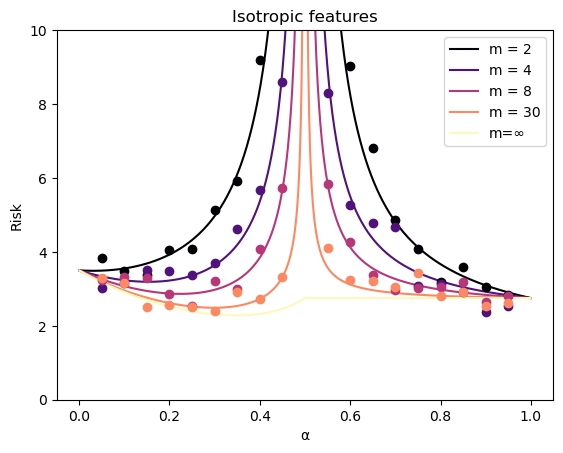
Figure 7: Asymptotic risk curves in (21) for linear ensemble estimator, when $m$ varies from $2$ to $30$, $\eta=1$, $r^{2}=3.5$ and $\sigma^{2}=1$. For each value of $m$, the points denote finite-sample risks averaged over $300$ experiments, with $n=200$, across various values of $\alpha$, computed from features $X$ that is $200\times 400$ matrix and have i.i.d. $N(0,1)$ entries.

Figure 8: Asymptotic risk curves in (21) for linear ensemble estimator, when $m$ varies from $2$ to $30$, $\eta=0.6$, $r^{2}=3.5$ and $\sigma^{2}=1$. For each value of $m$, the points denote finite-sample risks averaged over $300$ experiments, with $n=200$, across various values of $\alpha$, computed from features $X$ that is $200\times 400$ matrix and have i.i.d. $N(0,1)$ entries.

4 Conclusion

In this study, we derived higher-dimensional asymptotic limits for model averaging estimator, as well as a method for determining the optimal weights. As a result, we demonstrated that the double descent phenomenon occurs in model averaging estimators under certain conditions. Although many previous studies on model averaging methods achieved optimal weighting by minimizing certain criteria, we developed a method to calculate optimal weights directly by computing the asymptotic values of the predicted risk. We also note that the risk considered in this study was slightly different from those reported in previous studies (e.g., Hansen, (2007); Ando and Li, (2014)). Whereas those studies focused on minimizing the estimated in-sample risk, we developed a framework with the objective of minimizing the out-of-sample estimated risk.

Subsequent studies will include a derivation of better estimators of the signal-to-noise ratios $\mathrm{SNR}_{i}$ and $\mathrm{SNR}_{ij}$ for each candidate model in Corollary 2.4; although we derived a consistent estimator, its convergence rate were very slow numerically. In addition, it is important to consider the case where $\Sigma\neq I$. To this end, we believe that the results of the general sample covariance matrix deduced in Yin, (2018, 2022) can be extended further.

5 Acknowledgement

This work was supported by JSPS KAKENHI Grant Number 22H00510, and AMED Grant Numbers JP23dm0207001 and JP23dm0307009.

A Appendix

We now prove Theorem 2.1.

A.1 Proof of Theorem 2.1

A.1.1 Proof sketch for Theorem 2.1

We first briefly describe the proof of Theorem 2.1.

proof sketch for Theorem 2.1.

Let $|T_{i}|=n_{i}$, $|S_{i}|=p_{i}$, $|T_{i}\cap T_{j}|=n_{ij}$ and $|S_{i}\cap S_{j}|=p_{ij}$. First, we consider the ridge regression estimator $\hat{\beta}_{w_{n},\lambda}$ as follows:

$$\hat{\beta}_{w_{n},\lambda,k}=\sum_{i=1}^{m}w_{n,i}\mathbbm{1}_{\{i\in S_{i}\}}\hat{\beta}^{T_{i}}_{S_{i},\lambda,k},$$

where $\hat{\beta}_{w,\lambda,k}$ is the $k$-th component of $\hat{\beta}_{w_{n},\lambda}$ and $\hat{\beta}^{T_{i}}_{S_{i},\lambda}=\frac{1}{n_{i}}(\frac{1}{n_{i}}X^{T_{i}\top}_{S_{i}}X^{T_{i}}_{S_{i}}+\lambda\mathrm{I})^{-1}X^{T_{i}\top}_{S_{i}}y_{T_{i}}$, for $i=1,...,m$, $\lambda>0$. Define

$$B_{D}(\hat{\beta}_{w_{n},\lambda}) =\sum_{i=1}^{m}w_{n,i}^{2}\lambda^{2}\beta_{S_{i}}^{\top}\left(\frac{1}{n_{i}}X^{T_{i}\top}_{S_{i}}X^{T_{i}}_{S_{i}}+\lambda I\right)^{-2}\beta_{S_{i}},$$

$$V_{D}(\hat{\beta}_{w_{n},\lambda}) =\sum_{i=1}^{m}w_{n,i}^{2}\frac{\sigma^{2}}{n_{i}^{2}}\mathrm{Tr}\left(X^{T_{i}}_{S_{i}}\left(\frac{1}{n_{i}}X^{T_{i}\top}_{S_{i}}X^{T_{i}}_{S_{i}}+\lambda\mathrm{I}\right)^{-2}X^{T_{i}\top}_{S_{i}}\right)$$

$$B_{N}(\hat{\beta}_{w_{n},\lambda}) =\sum_{i,j,i\neq j}w_{n,i}w_{n,j}\lambda^{2}\beta_{S_{i}}^{\top}\left(\frac{1}{n_{i}}X^{T_{i}\top}_{S_{i}}X^{T_{i}}_{S_{i}}+\lambda\mathrm{I}\right)^{-1}E_{i,j}\left(\frac{1}{n_{j}}X^{T_{j}\top}_{S_{j}}X^{T_{j}}_{S_{j}}+\lambda\mathrm{I}\right)^{-1}\beta_{S_{j}},$$

$$V_{N}(\hat{\beta}_{w,\lambda}) =\sum_{i,j,i\neq j}w_{n,i}w_{n,j}\frac{\sigma^{2}}{n_{i}n_{j}}\mathrm{Tr}\left(X^{T_{i}\cap T_{j}}_{S_{i}}\left(\frac{1}{n}X^{T_{i}\top}_{S_{i}}X^{T_{i}}_{S_{i}}+\lambda\mathrm{I}\right)^{-1}E_{i,j}\left(\frac{1}{n}X^{T_{j}\top}_{S_{j}}X^{T_{j}}_{S_{j}}+\lambda\mathrm{I}\right)^{-1}X^{T_{i}\cap T_{j}\top}_{S_{j}}\right),$$

where $E_{i,j}=\mathbb{E}\left[x_{0,S_{i}}x_{0,S_{j}}^{\top}\right]$, $B_{D}(\hat{\beta}_{w_{n},\lambda})$ and $V_{D}(\hat{\beta}_{w_{n},\lambda})$ correspond to “diagonal component”, representing a kind of covariance between the same linear models, and $B_{N}(\hat{\beta}_{w_{n},\lambda})$ and $V_{N}(\hat{\beta}_{w_{n},\lambda})$ correspond to “off-diagonal component”, representing a kind of covariance between different linear models. Then

$$R_{X}(\hat{\beta}_{w_{n},\lambda})=B_{D}(\hat{\beta}_{w_{n},\lambda})+V_{D}(\hat{\beta}_{w_{n},\lambda})+B_{N}(\hat{\beta}_{w_{n},\lambda})+V_{N}(\hat{\beta}_{w_{n},\lambda}).$$ (22)

Observing the above terms, it is apparent that Lemma A.7 can be applied. Subsequently, Lemma A.6 can be used to complete the proof. ∎

A.1.2 Detailed proof of Theorem 2.1

Proof of Theorem 2.1.

In the following, we focus on $B_{D}(\hat{\beta}_{w_{n},\lambda}),V_{D}(\hat{\beta}_{w_{n},\lambda}),B_{N}(\hat{\beta}_{w_{n},\lambda})$ and $V_{N}(\hat{\beta}_{w_{n},\lambda})$. For the notation convenience, let

$$e_{l}(-\lambda)=\frac{-1+\frac{p_{l}}{n_{l}}-\lambda+\sqrt{(1-\frac{p_{l}}{n_{l}}+\lambda)^{2}+4p_{l}\lambda/n_{l}}}{2p_{l}\lambda/n_{l}},$$ (23)

for $l=1,2,...,m$. Thus, when $\frac{p_{l}}{n_{l}}<1$,

$$\lim_{\lambda\to 0}e_{l}(-\lambda)=\frac{1}{1-\frac{p_{l}}{n_{l}}},$$ (24)

on the other hand, when $\frac{p_{l}}{n_{l}}>1$,

$$\lim_{\lambda\to 0}\lambda e_{l}(-\lambda)=1-\frac{n_{l}}{p_{l}}.$$ (25)

Note that from Theorem 1 and its corollary of Bai and Silverstein, (1998) (see also Chapter 6 of Bai and Silverstein, (2010)), the largest and smallest nonzero eigenvalues of $X^{T_{i}\top}_{S_{i}}X^{T_{i}}_{S_{i}}$ have upper and lower constant bounds $M$ and $1/M$ independent of $i$ and $p$, respectively, for all large $n$. Hence, because $\sum_{i=1}^{n}w_{i}=1$, $B_{D}(\hat{\beta}_{w_{n},\lambda}),V_{D}(\hat{\beta}_{w_{n},\lambda}),B_{N}(\hat{\beta}_{w_{n},\lambda})$ and $V_{N}(\hat{\beta}_{w_{n},\lambda})$ are all upper-bounded by a constant for all large $n$ and $\lambda>0$. Furthermore, we can also bound the derivative of $B_{D}(\hat{\beta}_{w_{n},\lambda}),V_{D}(\hat{\beta}_{w_{n},\lambda}),B_{N}(\hat{\beta}_{w_{n},\lambda})$ and $V_{N}(\hat{\beta}_{w_{n},\lambda})$ from above.

We first consider the case wherein $\gamma_{i}<\eta_{i},\gamma_{j}<\eta_{j}$ for any $i,j$. From Theorem 1 and its Corollary in Bai and Silverstein, (1998) (see also chapter 6 of Bai and Silverstein, (2010)), all eigenvalues of $X^{T_{i}\top}_{S_{i}}X^{T_{i}}_{S_{i}}$ are bounded away from 0 for all large $n$ almost surely, $B_{D}(\hat{\beta}_{w_{n},\lambda})\to 0$, $B_{N}(\hat{\beta}_{w_{n},\lambda})\to 0$ as $\lambda\to 0$. Therefore, we only need to focus on the variance terms. From (9) in Theorem 1 of Hastie et al., (2022), $V_{D}(\hat{\beta}_{w_{n},\lambda})\to\sum_{i=1}^{m}w_{i}^{2}\frac{\gamma_{i}}{1-\gamma_{i}}$ as $n\to\infty,\lambda\to 0$. For the term $V_{N}(\hat{\beta}_{w_{n},\lambda})$, Lemmas A.6 and A.7 help us obtain its asymptotic behavior. If we replace $Z_{1}$ with $X_{S_{i}}^{T_{i}}$ and $Z_{2}$ with $X^{T_{j}}_{S_{j}}$ in Lemma A.7, we obtain

$$V_{N}(\hat{\beta}_{w_{n},\lambda}) =\sum_{i,j,i\neq j}w_{n,i}w_{n,j}\sigma^{2}\frac{1}{n_{i}n_{j}}\mathrm{Tr}\left\{X_{S_{i}}^{T_{i}\cap T_{j}}\left(\frac{1}{n_{i}}X_{S_{i}}^{T_{i}\top}X_{S_{i}}^{T_{i}}+\lambda\mathrm{I}\right)^{-1}E_{i,j}\left(\frac{1}{n_{j}}X_{S_{j}}^{T_{j}\top}X_{S_{j}}^{T_{j}}+\lambda\mathrm{I}\right)^{-1}X_{S_{j}}^{T_{i}\cap T_{j}\top}\right\}$$

$$=\frac{1}{n_{ij}}\sum_{i,j,i\neq j}w_{n,i}w_{n,j}\sigma^{2}\frac{\frac{n_{ij}}{n_{i}n_{j}}\mathrm{Tr}\left(\left(\frac{1}{n_{i}}X_{S_{i}}^{T_{i}\top}X_{S_{i}}^{T_{i}}+\lambda\mathrm{I}\right)^{-1}E_{i,j}\left(\frac{1}{n_{j}}X_{S_{j}}^{T_{j}\top}X_{S_{j}}^{T_{j}}+\lambda\mathrm{I}\right)^{-1}E_{i,j}^{\top}\right)}{\left(1+\frac{1}{n_{i}}\mathrm{Tr}\left(\left(\frac{1}{n}X_{S_{i}}^{T_{i}\top}X_{S_{i}}^{T_{i}}+\lambda\mathrm{I}\right)^{-1}\right)\right)\left(1+\frac{1}{n_{j}}\mathrm{Tr}\left(\left(\frac{1}{n_{j}}X_{S_{j}}^{T_{j}\top}X_{S_{j}}^{T_{j}}+\lambda\mathrm{I}\right)^{-1}\right)\right)}$$

$$\quad+o_{a.s.}(1).$$ (26)

Hence, by applying Lemma A.6 to (26), we obtain

$$V_{N}(\hat{\beta}_{w_{n},\lambda})=\sum_{i,j,i\neq j}w_{n,i}w_{n,j}\sigma^{2}\frac{\frac{n_{ij}p_{ij}}{n_{i}n_{j}}e_{i}(-\lambda)e_{j}(-\lambda)}{(1+\frac{p_{i}}{n_{i}}e_{i}(-\lambda))(1+\frac{p_{j}}{n_{j}}e_{j}(-\lambda))\left(1-\frac{\frac{n_{ij}p_{ij}}{n_{i}n_{j}}e_{i}(-\lambda)e_{j}(-\lambda)}{(1+\frac{p_{i}}{n_{i}}e_{i}(-\lambda))(1+\frac{p_{j}}{n_{j}}e_{j}(-\lambda))}\right)}\quad+o_{a.s.}(1).$$ (27)

As mentioned previously, $B_{D}(\hat{\beta}_{w_{n},\lambda}),V_{D}(\hat{\beta}_{w_{n},\lambda}),B_{N}(\hat{\beta}_{w_{n},\lambda})$ and $V_{N}(\hat{\beta}_{w_{n},\lambda})$ along with their derivatives, are all bounded away from $\infty$ and are equicontinuous and uniformly bounded in terms of $\lambda\geq 0$. Therefore we can apply Arzelà-Ascoli theorem to obtain the claim by $\lambda\to 0$ after $n,p\to\infty$.

Next, we consider the case where $\gamma_{i}<\eta_{i},\eta_{j}<\gamma_{j}$. Here, the asymptotic behavior of the variance term can be obtained in a manner similar to the case $\gamma_{i}<\eta_{i},\gamma_{j}<\eta_{j}$. From Theorem 1 and its Corollary in Bai and Silverstein, (1998) (see also chapter 6 of Bai and Silverstein, (2010)), the eigenvalues of $X^{T_{i}\top}_{S_{i}}X^{T_{i}}_{S_{i}}$ are bounded away from 0; Thus, $B_{D}\to 0$ and $B_{N}\to 0$ as $n,p\to\infty$ and $\lambda\to 0$. The cases in which $\gamma_{j}<\eta_{j},\eta_{i}<\gamma_{i}$ are similar.

Finally, we consider the case where $\eta_{i}<\gamma_{i},\eta_{j}<\gamma_{j}$. In this case, the same argument as in the previous two cases yields the asymptotic behavior of the variance term. As for the bias term $B_{D}(\hat{\beta}_{w_{n},\lambda})$, we can obtain the claim using an argument similar to the proof of Theorem 1 in Hastie et al., (2022). In terms of $B_{N}(\hat{\beta}_{w_{n},\lambda})$, by substituting $E_{12}$ into $\Theta_{1}$ and $\beta_{S_{j}}\beta_{S_{i}}^{\top}$ into $\Theta_{2}$ in Lemma A.6, we obtain

$$B_{N}(\hat{\beta}_{w_{n},\lambda}) =\sum_{i,j,i\neq j}w_{n,i}w_{n,j}\lambda^{2}\beta_{S_{i}}^{\top}\left(X^{T_{i}\top}_{S_{i}}X^{T_{i}}_{S_{i}}+\lambda\mathrm{I}\right)^{-1}E_{i,j}\left(X^{T_{j}\top}_{S_{j}}X^{T_{j}}_{S_{j}}+\lambda\mathrm{I}\right)^{-1}\beta_{S_{j}}$$

$$=\sum_{i,j,i\neq j}w_{n,i}w_{n,j}\left(\lambda^{2}e_{i}e_{j}\beta_{S_{i}}^{\top}E_{i,j}\beta_{S_{j}}+\lambda^{2}e_{i}e_{j}\frac{\beta_{S_{i}}^{\top}E_{i,j}\beta_{S_{j}}\frac{n_{ij}p_{ij}}{n_{i}n_{j}}e_{i}(-\lambda)e_{j}(-\lambda)}{(1+\frac{p_{i}}{n_{i}}e_{i})(1+\frac{p_{j}}{n_{j}}e_{j})\left(1-\frac{\frac{n_{ij}p_{ij}}{n_{i}n_{j}}e_{i}(-\lambda)e_{j}(-\lambda)}{(1+\frac{p_{i}}{n_{i}}e_{i}(-\lambda))(1+\frac{p_{j}}{n_{j}}e_{j}(-\lambda))}\right)}\right)+o_{a.s.}(1).$$ (28)

Therefore, by applying Arzelà-Ascoli theorem and $\lambda\to 0$ after $n,p\to\infty$, and performing some calculations, we obtain

$$B_{N}(\hat{\beta}_{w_{n}})\to\sum_{i,j,i\neq j}w_{i}w_{j}\frac{(\gamma_{i}-\eta_{j})(\gamma_{j}-\eta_{i})}{\gamma_{i}\gamma_{j}-\eta_{ij}\gamma_{ij}}r^{2}\kappa_{ij}.$$ (29)

This completes the proof.

∎

In the next, we prove Theorem 2.3.

A.2 proof of Theorem 2.3

A.2.1 Proof sketch for Theorem 2.3

proof sketch for Theorem 2.3.

Because analogous proofs can be used for the diagonal and off-diagonal components of $H_{\mathrm{mis}}$, we hereafter focus specifically on the off-diagonal part. The off-diagonal part can be written as

$$\mathbbm{E}\left[(\hat{\beta}^{T_{i}\top}_{S_{i}}x_{0,S_{i}}-\beta^{\top}x_{0})(\hat{\beta}^{T_{j}\top}_{S_{j}}x_{0,S_{j}}-\beta^{\top}x_{0})\right]$$

$$=\mathbbm{E}\left[(\hat{\beta}^{T_{i}\top}_{S_{i}}x_{0,S_{i}}-\beta_{S_{i}}^{\top}x_{0,S_{i}})(\hat{\beta}^{T_{j}\top}_{S_{j}}x_{0,S_{j}}-\beta_{S_{j}}^{\top}x_{0,S_{j}})\right]+\mathbbm{E}\left[(\beta_{S_{i}^{c}\cap S_{j}^{c}}^{\top}x_{0,S_{i}\cup S_{j}})^{2}\right]$$

$$\quad-\mathbbm{E}\left[(\hat{\beta}^{T_{i}\top}_{S_{i}}x_{0,S_{i}}-\beta_{S_{i}}^{\top}x_{0,S_{i}})\beta_{S_{i}\setminus S_{j}}^{\top}x_{0,S_{i}\setminus S_{j}}\right]-\mathbbm{E}\left[(\hat{\beta}^{T_{j}\top}_{S_{j}}x_{0,S_{j}}-\beta_{S_{j}}^{\top}x_{0,S_{j}})\beta_{S_{j}\setminus S_{i}}^{\top}x_{0,S_{j}\setminus S_{i}}\right]$$

$$=\Delta_{1}+\Delta_{2}+\Delta_{3}+\Delta_{4}+\Delta_{5}+\Delta_{6}+\Delta_{7}$$

where

$$\Delta_{1}=\mathbbm{E}\left[(\tilde{\beta}^{T_{i}}_{S_{i},S_{j}}-\beta_{S_{i}})^{\top}E_{i,j}(\tilde{\beta}^{T_{j}}_{S_{j},S_{i}}-\beta_{S_{j}})\right],$$ (30)

$$\Delta_{2}=\mathbbm{E}\left[\beta_{S_{j}\setminus S_{i}}^{\top}X^{T_{i}\top}_{S_{j}\setminus S_{i}}X^{T_{i}}_{S_{i}}(X^{T_{i}\top}_{S_{i}}X^{T_{i}}_{S_{i}})^{+}E_{i,j}(\tilde{\beta}^{T_{j}}_{S_{j},S_{i}}-\beta_{S_{j}})\right],$$ (31)

$$\Delta_{3}=\mathbbm{E}\left[(\tilde{\beta}^{T_{i}}_{S_{i},S_{j}}-\beta_{S_{i}})^{\top}E_{i,j}(X^{T_{j}\top}_{S_{j}}X^{T_{j}}_{S_{j}})^{+}X^{T_{j}\top}_{S_{j}}X^{T_{j}}_{S_{i}\setminus S_{j}}\beta_{S_{i}\setminus S_{j}}\right],$$ (32)

$$\Delta_{4}=\mathbbm{E}\left[\beta_{S_{j}\setminus S_{i}}^{\top}X^{T_{i}\top}_{S_{j}\setminus S_{i}}X^{T_{i}}_{S_{i}}(X^{T_{i}\top}_{S_{i}}X^{T_{i}}_{S_{i}})^{+}E_{i,j}(X^{T_{j}\top}_{S_{j}}X^{T_{j}}_{S_{j}})^{+}X^{T_{j}\top}_{S_{j}}X^{T_{j}}_{S_{i}\setminus S_{j}}\beta_{S_{i}\setminus S_{j}}\right],$$ (33)

$$\Delta_{5}=\mathbbm{E}\left[\left(\beta_{S_{i}^{c}\cap S_{j}^{c}}x_{0,S_{i}^{c}\cap S_{j}^{c}}\right)^{2}\right]=\|\beta_{S_{i}^{c}\cap S_{j}^{c}}\|^{2},$$ (34)

$$\Delta_{6}=\mathbbm{E}\left[(\beta_{S_{j}}-\hat{\beta}^{T_{j}}_{S_{j}})^{\top}F_{j,i}\beta_{S_{j}\setminus S_{i}}\right],$$ (35)

$$\Delta_{7}=\mathbbm{E}\left[(\beta_{S_{i}}-\hat{\beta}^{T_{i}}_{S_{i}})^{\top}F_{i,j}\beta_{S_{i}\setminus S_{j}}\right],$$ (36)

where $\tilde{\beta}^{T_{l}}_{S_{l},S_{m}}=(X^{T_{l}\top}_{S_{l}}X^{T_{l}}_{S_{l}})^{+}X^{T_{l}\top}_{S_{l}}(X^{T_{l}}_{S_{l}}\beta_{S_{l}}+X^{T_{l}}_{S_{l}^{c}\cap S_{m}^{c}}\beta_{S_{l}^{c}\cap S_{m}^{c}}+\epsilon_{T_{l}})$, $F_{l,m}=\mathbbm{E}\left[x_{0,S_{l}}x_{S_{l}\setminus S_{m}}^{\top}\right]$. For $\Delta_{1}$, because we can regard the term $X^{T_{l}}_{S_{l}^{c}\cap S_{m}^{c}}\beta_{S_{l}^{c}\cap S_{m}^{c}}+\epsilon_{T_{l}}$ of $\tilde{\beta}^{T_{l}}_{S_{l},S_{m}}$ as noise term, we can apply the same procedure as in the proof for Theorem 2.1. We need to obtain the limiting behavior of the rest of the terms $\Delta_{2},\Delta_{3},\Delta_{4},\Delta_{6}$ and $\Delta_{7}$. Because the derivation is somewhat involved, please refer to the following section for detail. ∎

A.2.2 Detailed proof of Theorem 2.3

proof of Theorem 2.3.

For $\Delta_{1}$, because we can regard the term $X^{T_{l}}_{S_{l}^{c}\cap S_{m}^{c}}\beta_{S_{l}^{c}\cap S_{m}^{c}}+\epsilon_{T_{l}}$ of $\tilde{\beta}^{T_{l}}_{S_{l},S_{m}}$ as the noise term, using the same procedure as in the proof for Theorem 2.1, we can obtain, as $n,p\to\infty$,

$$\Delta_{1}\to\begin{cases}\frac{\eta_{ij}\gamma_{ij}}{\eta_{i}\eta_{j}-\eta_{ij}\gamma_{ij}}(r^{2}(1-\kappa_{i}-\kappa_{j}+\kappa_{ij})+\sigma^{2})\quad&\gamma_{i}<\eta_{i},\gamma_{j}<\eta_{j},\\ \frac{\eta_{ij}\gamma_{ij}}{\eta_{i}\gamma_{j}-\eta_{ij}\gamma_{ij}}(r^{2}(1-\kappa_{i}-\kappa_{j}+\kappa_{ij})+\sigma^{2})\quad&\gamma_{i}<\eta_{i},\eta_{j}<\gamma_{j},\\ \frac{\eta_{ij}\gamma_{ij}}{\eta_{j}\gamma_{i}-\eta_{ij}\gamma_{ij}}(r^{2}(1-\kappa_{i}-\kappa_{j}+\kappa_{ij})+\sigma^{2})\quad&\gamma_{j}<\eta_{j},\eta_{i}<\gamma_{i},\\ \frac{(\gamma_{i}-\eta_{i})(\gamma_{j}-\eta_{j})}{\gamma_{i}\gamma_{j}-\eta_{ij}\gamma_{ij}}r^{2}\kappa_{ij}+\frac{\eta_{ij}\gamma_{ij}}{\gamma_{i}\gamma_{j}-\eta_{ij}\gamma_{ij}}(r^{2}(1-\kappa_{i}-\kappa_{j}+\kappa_{ij})+\sigma^{2})\quad&1<\gamma_{i},\gamma_{j},\end{cases}$$

along with bounded convergence theorem. On the terms $\Delta_{2},\Delta_{3}$, since

$$\Delta_{2} =\mathbbm{E}\left[\beta_{S_{j}\setminus S_{i}}^{\top}X^{T_{i}\top}_{S_{j}\setminus S_{i}}X^{T_{i}}_{S_{i}}(X^{T_{i}\top}_{S_{i}}X^{T_{i}}_{S_{i}})^{+}E_{i,j}(\tilde{\beta}^{T_{j}}_{S_{j},S_{i}}-\beta_{S_{j}})\right]$$

$$=\mathbbm{E}\left[\beta_{S_{j}\setminus S_{i}}^{\top}X^{T_{i}\top}_{S_{j}\setminus S_{i}}X^{T_{i}}_{S_{i}}(X^{T_{i}\top}_{S_{i}}X^{T_{i}}_{S_{i}})^{+}E_{i,j}\left(\left(X^{T_{j}\top}_{S_{j}}X^{T_{j}}_{S_{j}}\right)^{+}X^{T_{j}\top}_{S_{j}}X^{T_{j}}_{S_{j}}-I\right)\beta_{S_{j}}\right]$$

$$=\sum_{k\in T_{i}}\mathbbm{E}\left[x_{S_{i},k}^{\top}(X^{T_{i}\top}_{S_{i}}X^{T_{i}}_{S_{i}})^{+}E_{i,j}\left(\left(X^{T_{j}\top}_{S_{j}}X^{T_{j}}_{S_{j}}\right)^{+}X^{T_{j}\top}_{S_{j}}X^{T_{j}}_{S_{j}}-I\right)\beta_{S_{j}}\beta_{S_{j}\setminus S_{i}}^{\top}x_{S_{j}\setminus S_{i},k}\right],$$

$$\Delta_{3} =\mathbbm{E}\left[(\tilde{\beta}^{T_{i}}_{S_{i},S_{j}}-\beta_{S_{i}})^{\top}E_{i,j}(X^{T_{j}\top}_{S_{j}}X^{T_{j}}_{S_{j}})^{+}X^{T_{j}\top}_{S_{j}}X^{T_{j}}_{S_{i}\setminus S_{j}}\beta_{S_{i}\setminus S_{j}}\right]$$

$$=\mathbbm{E}\left[\beta_{S_{i}}^{\top}\left(X^{T_{i}\top}_{S_{i}}X^{T_{i}}_{S_{i}}(X^{T_{i}\top}_{S_{i}}X^{T_{i}}_{S_{i}})^{+}-\mathrm{I}\right)E_{i,j}(X^{T_{j}\top}_{S_{j}}X^{T_{j}}_{S_{j}})^{+}X^{T_{j}\top}_{S_{j}}X^{T_{j}}_{S_{i}\setminus S_{j}}\beta_{S_{i}\setminus S_{j}}\right]$$

$$=\sum_{k\in T_{j}}\mathbbm{E}\left[x_{S_{i}\setminus S_{j},k}^{\top}\beta_{S_{i}\setminus S_{j}}\beta_{S_{i}}^{\top}\left(X^{T_{i}\top}_{S_{i}}X^{T_{i}}_{S_{i}}(X^{T_{i}\top}_{S_{i}}X^{T_{i}}_{S_{i}})^{+}-\mathrm{I}\right)E_{i,j}(X^{T_{j}\top}_{S_{j}}X^{T_{j}}_{S_{j}})^{+}x_{S_{j},k}\right]$$

where $x_{k}$ denotes the $k$-th row vector of $X$. Let us consider

$$\delta_{2,k}(\lambda)=\delta_{2,k}=-\lambda x_{S_{i},k}^{\top}Q_{i}E_{i,j}Q_{j}\beta_{S_{j}}\beta_{S_{j}\setminus S_{i}}^{\top}x_{S_{j}\setminus S_{i},k},$$ (37)

for $\lambda\geq 0$, where $Q_{i}(\lambda)=\left(\frac{1}{n_{i}}X^{T_{i}\top}_{S_{i}}X^{T_{i}}_{S_{i}}+\lambda\mathrm{I}\right)^{-1}$ and $Q_{j}(\lambda)=\left(\frac{1}{n_{j}}X^{T_{j}\top}_{S_{j}}X^{T_{j}}_{S_{j}}+\lambda\mathrm{I}\right)^{-1}$. Furthermore, we define $Q_{i,(k)}(\lambda)=\left(\frac{1}{n_{i}}X^{T_{i}\top}_{S_{i},(k)}X^{T_{i}}_{S_{i},(k)}+\lambda\mathrm{I}\right)^{-1}$ and $Q_{j,(k)}(\lambda)=\left(\frac{1}{n_{j}}X^{T_{j}\top}_{S_{j},(k)}X^{T_{j}}_{S_{j},(k)}+\lambda\mathrm{I}\right)^{-1}$, where $X_{(k)}$ denotes the $(n-1)\times p$ matrix excluding the $k$-th row vector of an $n\times p$ matrix $X$. Note that,

$$\mathbbm{E}\left[\lim_{\lambda\to 0}\frac{1}{n_{i}}\sum_{k\in T_{i}}\delta_{2,k}\right]=\mathbbm{E}\left[\lim_{\lambda\to 0}\frac{1}{n_{i}}\sum_{k\in T_{i}}-\lambda x_{S_{i},k}^{\top}Q_{i}E_{i,j}Q_{j}\beta_{S_{j}}\beta_{S_{j}\setminus S_{i}}^{\top}x_{S_{j}\setminus S_{i},k}\right]=\Delta_{2}.$$ (38)

and $\frac{1}{n_{i}}\sum_{k\in T_{i}}\delta_{2,k}$ can be uniformly bounded from above on $\lambda\in\left[0,C\right]$ for $n$ large enough and a positive real number $C>0$. This can be seen from the results of Theorem 1 and its corollary in Bai and Silverstein, (1998). If $k\in T_{1}\cap T_{2}$, we can obtain

$$\delta_{2,k} =-\lambda x_{S_{i},k}^{\top}Q_{i}E_{i,j}Q_{j}\beta_{S_{j}}\beta_{S_{j}\setminus S_{i}}^{\top}x_{S_{j}\setminus S_{i},k}$$

$$=-\lambda\frac{x_{S_{i},k}^{\top}Q_{i,(k)}E_{i,j}Q_{j,(k)}\beta_{S_{j}}\beta_{S_{j}\setminus S_{i}}^{\top}x_{S_{j}\setminus S_{i},k}}{\left(1+\frac{1}{n_{i}}x_{S_{i},k}^{\top}Q_{i,(k)}x_{S_{i},k}\right)}+\lambda\frac{\frac{1}{n_{j}}x_{S_{i},k}^{\top}Q_{i,(k)}E_{i,j}Q_{j,(k)}x_{S_{j},k}x_{S_{j},k}^{\top}Q_{j,(k)}\beta_{S_{j}}\beta_{S_{j}\setminus S_{i}}^{\top}x_{S_{j}\setminus S_{i},k}}{\left(1+\frac{1}{n_{i}}x_{S_{i},k}^{\top}Q_{i,(k)}x_{S_{i},k}\right)\left(1+\frac{1}{n_{j}}x_{S_{j},k}^{\top}Q_{j,(k)}x_{S_{j},k}\right)}.$$ (39)

Furthermore,

$$\mathbbm{E}\left[\left|\lambda\frac{x_{S_{i},k}^{\top}Q_{i,(k)}E_{i,j}Q_{j,(k)}\beta_{S_{j}}\beta_{S_{j}\setminus S_{i}}^{\top}x_{S_{j}\setminus S_{i},k}}{\left(1+\frac{1}{n_{i}}x_{S_{i},k}^{\top}Q_{i,(k)}x_{S_{i},k}\right)}-\lambda\frac{x_{S_{i},k}^{\top}Q_{i,(k)}E_{i,j}Q_{j,(k)}\beta_{S_{j}}\beta_{S_{j}\setminus S_{i}}^{\top}x_{S_{j}\setminus S_{i},k}}{\left(1+\frac{1}{n_{i}}\mathrm{Tr}\left(Q_{i,(k)}\right)\right)}\right|^{q}\right]=O\left(\frac{1}{n^{q/2}}\right),$$ (40)

$$\mathbbm{E}\left[\left|\lambda\frac{\frac{1}{n_{j}}x_{S_{i},k}^{\top}Q_{i,(k)}E_{i,j}Q_{j,(k)}x_{S_{j},k}x_{S_{j},k}^{\top}Q_{j,(k)}\beta_{S_{j}}\beta_{S_{j}\setminus S_{i}}^{\top}x_{S_{j}\setminus S_{i},k}}{\left(1+\frac{1}{n_{i}}x_{S_{i},k}^{\top}Q_{i,(k)}x_{S_{i},k}\right)\left(1+\frac{1}{n_{j}}x_{S_{j},k}^{\top}Q_{j,(k)}x_{S_{j},k}\right)}\right.\right.$$ (41)

$$\quad-\left.\left.\lambda\frac{\frac{1}{n_{j}}\mathrm{Tr}\left(Q_{i,(k)}E_{i,j}Q_{j,(k)}E_{i,j}^{\top}\right)x_{S_{j},k}^{\top}Q_{j,(k)}\beta_{S_{j}}\beta_{S_{j}\setminus S_{i}}^{\top}x_{S_{j}\setminus S_{i},k}}{\left(1+\frac{1}{n_{i}}\mathrm{Tr}\left(Q_{i,(k)}\right)\right)\left(1+\frac{1}{n_{j}}\mathrm{Tr}\left(Q_{j,(k)}\right)\right)}\right|^{q}\right]=O\left(\frac{1}{n^{q/2}}\right),$$ (42)

by combining Lemmas A.4, A.5, A.2 with the Cauchy-Schwartz inequality. On the other hand, if $k\in T_{i}\setminus T_{j}$, we can obtain

$$\delta_{2,k} =-\lambda x_{S_{i},k}^{\top}Q_{i}E_{i,j}Q_{j}\beta_{S_{j}}\beta_{S_{j}\setminus S_{i}}^{\top}x_{S_{j}\setminus S_{i},k}$$

$$=-\lambda\frac{x_{S_{i},k}^{\top}Q_{i,(k)}E_{i,j}Q_{j}\beta_{S_{j}}\beta_{S_{j}\setminus S_{i}}^{\top}x_{S_{j}\setminus S_{i},k}}{\left(1+\frac{1}{n}x_{S_{i},k}^{\top}Q_{i,(k)}x_{S_{i},k}\right)}$$ (43)

and

$$\mathbbm{E}\left[\left|\lambda\frac{x_{S_{i},k}^{\top}Q_{i,(k)}E_{i,j}Q_{j}\beta_{S_{j}}\beta_{S_{j}\setminus S_{i}}^{\top}x_{S_{j}\setminus S_{i},k}}{\left(1+\frac{1}{n_{i}}x_{S_{i},k}^{\top}Q_{i,(k)}x_{S_{i},k}\right)}-\lambda\frac{x_{S_{i},k}^{\top}Q_{i,(k)}E_{i,j}Q_{j}\beta_{S_{j}}\beta_{S_{j}\setminus S_{i}}^{\top}x_{S_{j}\setminus S_{i},k}}{\left(1+\frac{1}{n_{i}}\mathrm{Tr}\left(Q_{i,(k)}\right)\right)}\right|^{q}\right]=O\left(\frac{1}{n^{q/2}}\right).$$ (44)

Thus we obtain

$$\Delta_{2}\to\begin{cases}0\quad&\gamma_{j}<\eta_{j},\\ \frac{\eta_{ij}\gamma_{ij}(\gamma_{j}-\eta_{j})}{\gamma_{j}(\eta_{i}\gamma_{j}-\eta_{ij}\gamma_{ij})}r^{2}(\kappa_{j}-\kappa_{ij})\quad&\gamma_{i}<\eta_{i},\eta_{j}<\gamma_{j},\\ \frac{\eta_{ij}\gamma_{ij}(\gamma_{j}-\eta_{j})}{\gamma_{j}(\gamma_{i}\gamma_{j}-\eta_{ij}\gamma_{ij})}r^{2}(\kappa_{j}-\kappa_{ij})\quad&\eta_{i}<\gamma_{i},\eta_{j}<\gamma_{j},\end{cases}$$ (45)

with Lemma A.6, Lemma A.3, Arzèla-Ascoli theorem, and the bounded convergence theorem. $\Delta_{3}\to 0$ can be shown similarly. The term $\Delta_{4}$ can be rewritten as:

$$\Delta_{4} =\mathbbm{E}\left[\beta_{S_{j}\setminus S_{i}}^{\top}X^{T_{i}\top}_{S_{j}\setminus S_{i}}X^{T_{i}}_{S_{i}}(X^{T_{i}\top}_{S_{i}}X^{T_{i}}_{S_{i}})^{+}E_{i,j}(X^{T_{j}\top}_{S_{j}}X^{T_{j}}_{S_{j}})^{+}X^{T_{j}\top}_{S_{j}}X^{T_{j}}_{S_{i}\setminus S_{j}}\beta_{S_{i}\setminus S_{j}}\right]$$

$$=\frac{1}{n_{ij}}\sum_{k\in T_{i}\cap T_{j}}\frac{n_{ij}}{n_{i}n_{j}}\left(\mathbbm{E}\left[x_{S_{i},k}^{\top}\left(\frac{1}{n_{i}}X^{T_{i}\top}_{S_{i}}X^{T_{i}}_{S_{i}}\right)^{+}E_{i,j}\left(\frac{1}{n_{j}}X^{T_{j}\top}_{S_{j}}X^{T_{j}}_{S_{j}}\right)^{+}X^{T_{j}\top}_{S_{j},(k)}X^{T_{j}}_{S_{i}\setminus S_{j},(k)}\beta_{S_{i}\setminus S_{j}}\beta_{S_{j}\setminus S_{i}}^{\top}x_{S_{j}\setminus S_{i},k}\right]\right.$$

$$\quad\left.+\mathbbm{E}\left[x_{S_{i},k}^{\top}\left(\frac{1}{n_{i}}X_{S_{i}}^{\top}X_{S_{i}}\right)^{+}E_{i,j}\left(\frac{1}{n_{j}}X^{T_{j}\top}_{S_{j}}X^{T_{j}}_{S_{j}}\right)^{+}x_{S_{j},k}x_{S_{i}\setminus S_{j},k}^{\top}\beta_{S_{i}\setminus S_{j}}\beta_{S_{j}\setminus S_{i}}^{\top}x_{S_{j}\setminus S_{i},k}\right]\right)$$

$$\quad+\frac{1}{n_{ij}}\sum_{k\in T_{i}\setminus T_{j}}\frac{n_{ij}}{n_{i}n_{j}}\mathbbm{E}\left[x_{S_{i},k}^{\top}\left(\frac{1}{n_{i}}X^{T_{i}\top}_{S_{i}}X^{T_{i}}_{S_{i}}\right)^{+}E_{i,j}\left(\frac{1}{n_{j}}X^{T_{j}\top}_{S_{j}}X^{T_{j}}_{S_{j}}\right)^{+}X^{T_{j}\top}_{S_{j}}X^{T_{j}}_{S_{i}\setminus S_{j}}\beta_{S_{i}\setminus S_{j}}\beta_{S_{j}\setminus S_{i}}^{\top}x_{S_{j}\setminus S_{i},k}\right]$$

$$=\Delta_{41}+\Delta_{42}+\Delta_{43},$$

For $\Delta_{4}\to 0$, we consider the following:

$$\delta_{41,k}(\lambda)=\delta_{41,k}=\frac{n_{ij}}{n_{i}n_{j}}x_{S_{i},k}^{\top}Q_{i}E_{i,j}Q_{j}X_{S_{j},(k)}^{\top}X_{S_{i}\setminus S_{j},(k)}\beta_{S_{i}\setminus S_{j}}\beta_{S_{j}\setminus S_{i}}^{\top}x_{S_{j}\setminus S_{i},k}$$ (46)

$$\delta_{42,k}(\lambda)=\delta_{42,k}=\frac{n_{ij}}{n_{i}n_{j}}x_{S_{i},k}^{\top}Q_{i}E_{i,j}Q_{j}x_{S_{j},k}x_{S_{i}\setminus S_{j},k}^{\top}\beta_{S_{i}\setminus S_{j}}\beta_{S_{j}\setminus S_{i}}^{\top}x_{S_{j}\setminus S_{i},k}$$ (47)

for $\lambda>0$. We assume that $k\in T_{i}\cap T_{j}$. Note that

$$\mathbbm{E}\left[\lim_{\lambda\to 0}\sum_{k\in T_{i}\cap T_{j}}\delta_{41,k}\right]=\Delta_{41}$$

$$\mathbbm{E}\left[\lim_{\lambda\to 0}\sum_{k\in T_{i}\cap T_{j}}\delta_{42,k}\right]=\Delta_{42},$$

and $\sum_{k\in T_{i}\cap T_{j}}\delta_{41,k}$ and $\sum_{k\in T_{i}\cap T_{j}}\delta_{42,k}$ are uniformly bounded on $\lambda\in[0,C]$ for a positive real number $C$. First, we demonstrate that $\Delta_{42}\to 0$. Using the technique in the proof of Theorem 2.1, we obtain

$$\mathbbm{E}\left[\left|\delta_{42,k}-\frac{\frac{n_{ij}}{n_{i}n_{j}}\mathrm{Tr}\left(Q_{i,(k)}E_{i,j}Q_{j,(k)}E_{i,j}^{\top}\right)}{(1+\frac{1}{n_{i}}\mathrm{Tr}\left(Q_{i,(k)}\right))(1+\frac{1}{n_{j}}\mathrm{Tr}\left(Q_{j,(k)}\right))}x_{S_{i}\setminus S_{j},k}^{\top}\beta_{S_{i}\setminus S_{j}}\beta_{S_{j}\setminus S_{i}}^{\top}x_{S_{j}\setminus S_{i},k}\right|^{q}\right]$$

$$=\mathbbm{E}\left[\left|\left(\frac{n_{ij}}{n_{i}n_{j}}x_{S_{i},k}^{\top}Q_{i}E_{i,j}Q_{j}x_{S_{j},k}-\frac{\frac{n_{ij}}{n_{i}n_{j}}\mathrm{Tr}\left(Q_{i,(k)}E_{i,j}Q_{j,(k)}E_{i,j}^{\top}\right)}{(1+\frac{1}{n_{i}}\mathrm{Tr}\left(Q_{i,(k)}\right))(1+\frac{1}{n_{j}}\mathrm{Tr}\left(Q_{j,(k)}\right))}\right)x_{S_{i}\setminus S_{j},k}^{\top}\beta_{S_{i}\setminus S_{j}}\beta_{S_{j}\setminus S_{i}}^{\top}x_{S_{j}\setminus S_{i},k}\right|^{q}\right]$$

$$\leq\mathbbm{E}^{1/2}\left[\left|\frac{n_{ij}}{n_{i}n_{j}}x_{S_{i},k}^{\top}Q_{i}E_{i,j}Q_{j}x_{S_{j},k}-\frac{\frac{n_{ij}}{n_{i}n_{j}}\mathrm{Tr}\left(Q_{i,(k)}E_{i,j}Q_{j,(k)}E_{i,j}^{\top}\right)}{(1+\frac{1}{n_{i}}\mathrm{Tr}\left(Q_{i,(k)}\right))(1+\frac{1}{n_{j}}\mathrm{Tr}\left(Q_{j,(k)}\right))}\right|^{2q}\right]$$

$$\quad\quad\quad\quad\times\mathbbm{E}^{1/2}\left[\left|x_{S_{i}\setminus S_{j},k}^{\top}\beta_{S_{i}\setminus S_{j}}\beta_{S_{j}\setminus S_{i}}^{\top}x_{S_{j}\setminus S_{i},k}\right|^{2q}\right]$$ (48)

The first term in (48) can be written as

$$\mathbbm{E}^{1/2}\left[\left|\frac{n_{ij}}{n_{i}n_{j}}x_{S_{i},k}^{\top}Q_{i}E_{i,j}Q_{j}x_{S_{j},k}-\frac{\frac{n_{ij}}{n_{i}n_{j}}\mathrm{Tr}\left(Q_{i,(k)}E_{i,j}Q_{j,(k)}E_{i,j}^{\top}\right)}{(1+\frac{1}{n_{i}}\mathrm{Tr}\left(Q_{i,(k)}\right))(1+\frac{1}{n_{j}}\mathrm{Tr}\left(Q_{j,(k)}\right))}\right|^{2q}\right]$$

$$=\mathbbm{E}^{1/2}\left[\left|\frac{\frac{n_{ij}}{n_{i}n_{j}}x_{S_{i},k}^{\top}Q_{i,(k)}E_{i,j}Q_{j,(k)}x_{S_{j},k}}{(1+\frac{1}{n_{i}}x_{S_{i},k}^{\top}Q_{i,(k)}x_{S_{i},k})(1+\frac{1}{n_{j}}x_{S_{j},k}^{\top}Q_{j,(k)}x_{S_{j},k})}-\frac{\frac{n_{ij}}{n_{i}n_{j}}\mathrm{Tr}\left(Q_{i,(k)}E_{i,j}Q_{j,(k)}E_{i,j}^{\top}\right)}{(1+\frac{1}{n_{i}}\mathrm{Tr}\left(Q_{i,(k)}\right))(1+\frac{1}{n_{j}}\mathrm{Tr}\left(Q_{j,(k)}\right))}\right|^{2q}\right]$$

$$=O\left(\frac{1}{n^{q/2}}\right)$$ (49)

In (49), we use Lemma A.4 and Lemma A.5. Hence, from Lemma A.3 and Remark 1, we obtain

$$\frac{1}{n_{ij}}\mathbbm{E}\left[\sum_{k\in T_{i}\cap T_{j}}\frac{\frac{n_{ij}}{n_{i}n_{j}}\mathrm{Tr}\left(Q_{i,(k)}E_{i,j}Q_{j,(k)}E_{i,j}^{\top}\right)}{(1+\frac{1}{n_{i}}\mathrm{Tr}\left(Q_{i,(k)}\right))(1+\frac{1}{n_{j}}\mathrm{Tr}\left(Q_{j,(k)}\right))}x_{S_{i}\setminus S_{j},k}^{\top}\beta_{S_{i}\setminus S_{j}}\beta_{S_{j}\setminus S_{i}}^{\top}x_{S_{j}\setminus S_{i},k}\right]\to 0.$$ (50)

$\Delta_{42}\to 0$ follows by applying Arzèla-Ascoli theorem and bounded convergence theorem. Next, we consider the term $\delta_{41,k}$. Observing

$$\delta_{41,k} =\frac{n_{ij}}{n_{i}n_{j}}x_{S_{i},k}^{\top}Q_{i}E_{i,j}Q_{j}X^{T_{j}\top}_{S_{j},(k)}X^{T_{j}}_{S_{i}\setminus S_{j},(k)}\beta_{S_{i}\setminus S_{j}}\beta_{S_{j}\setminus S_{i}}^{\top}x_{S_{j}\setminus S_{i},k}$$

$$=\frac{n_{ij}}{n_{i}n_{j}}\frac{x_{S_{i},k}^{\top}Q_{i,(k)}E_{i,j}Q_{j,(k)}X^{T_{j}\top}_{S_{j},(k)}X^{T_{j}}_{S_{i}\setminus S_{j},(k)}\beta_{S_{i}\setminus S_{j}}\beta_{S_{j}\setminus S_{i}}^{\top}x_{S_{j}\setminus S_{i},k}}{(1+\frac{1}{n_{i}}x_{S_{i},k}^{\top}Q_{i,(k)}x_{S_{i},k})}$$

$$\quad\quad-\frac{n_{ij}}{n_{i}n_{j}^{2}}\frac{x_{S_{i},k}^{\top}Q_{i,(k)}E_{i,j}Q_{j,(k)}x_{S_{j},k}x_{S_{j},k}^{\top}Q_{j,(k)}X^{T_{j}\top}_{S_{j},(k)}X^{T_{j}}_{S_{i}\setminus S_{j},(k)}\beta_{S_{i}\setminus S_{j}}\beta_{S_{j}\setminus S_{i}}^{\top}x_{S_{j}\setminus S_{i},k}}{(1+\frac{1}{n_{i}}x_{S_{i},k}^{\top}Q_{i,(k)}x_{S_{i},k})(1+\frac{1}{n_{j}}x_{S_{j},k}^{\top}Q_{j,(k)}x_{S_{j},k})},$$ (51)

the expectation of the first term in (51) converges to $0$ by using the procedure similar to $\delta_{42,k}$. For the second term of (51), we first obtain

$$\mathbbm{E}\left[\left|\delta_{41,k}\right|^{q}\right]$$

$$=\mathbbm{E}\left[\left|\frac{n_{ij}}{n_{i}n_{j}^{2}}\frac{x_{S_{i},k}^{\top}Q_{i,(k)}E_{i,j}Q_{j,(k)}x_{S_{j},k}x_{S_{j},k}^{\top}Q_{j,(k)}X^{T_{j}\top}_{S_{j},(k)}X^{T_{j}}_{S_{i}\setminus S_{j},(k)}\beta_{S_{i}\setminus S_{j}}\beta_{S_{j}\setminus S_{i}}^{\top}x_{S_{j}\setminus S_{i},k}}{(1+\frac{1}{n_{i}}x_{S_{i},k}^{\top}Q_{i,(k)}x_{S_{i},k})(1+\frac{1}{n_{j}}x_{S_{j},k}^{\top}Q_{j,(k)}x_{S_{j},k})}\right.\right.$$

$$\quad\quad\left.\left.-\frac{n_{ij}}{n_{i}n_{j}^{2}}\frac{\mathrm{Tr}\left(Q_{i,(k)}E_{i,j}Q_{j,(k)}E_{i,j}^{\top}\right)x_{S_{j},k}^{\top}Q_{j,(k)}X^{T_{j}\top}_{S_{j},(k)}X^{T_{j}}_{S_{i}\setminus S_{j},(k)}\beta_{S_{i}\setminus S_{j}}\beta_{S_{j}\setminus S_{i}}^{\top}x_{S_{j}\setminus S_{i},k}}{(1+\frac{1}{n_{i}}\mathrm{Tr}(Q_{i,(k)}))(1+\frac{1}{n_{j}}\mathrm{Tr}(Q_{j,(k)}))}\right|^{q}\right]=O\left(\frac{1}{n^{q/2}}\right).$$ (52)

from Lemmas A.4 and A.3 along with the Cauchy-Schwartz inequality and the fact

$$\mathbbm{E}\left[\left|\frac{1}{n_{j}}x_{S_{j},k}^{\top}Q_{j,(k)}X^{T_{j}\top}_{S_{j},(k)}X^{T_{j}}_{S_{i}\setminus S_{j},(k)}\beta_{S_{i}\setminus S_{j}}\beta_{S_{j}\setminus S_{i}}^{\top}x_{S_{j}\setminus S_{i},k}\right|^{2q}\right]$$

$$\leq C_{q}\|\beta_{S_{j}\setminus S_{i}}\|^{q}\mathbbm{E}\left[\left|\frac{1}{n_{j}^{2}}\beta_{S_{i}\setminus S_{j}}^{\top}X^{T_{j}\top}_{S_{i}\setminus S_{j},(k)}X^{T_{j}}_{S_{j},(k)}Q_{j,(k)}^{2}X^{T_{j}\top}_{S_{j},(k)}X^{T_{j}}_{S_{i}\setminus S_{j},(k)}\beta_{S_{i}\setminus S_{j}}\right|^{q}\right]$$ (53)

$$\leq\frac{1}{\lambda^{2}}D_{q}\|\beta_{S_{j}\setminus S_{i}}\|^{q}\mathbbm{E}\left[\left|\frac{1}{n_{j}}\beta_{S_{i}\setminus S_{j}}^{\top}X^{T_{j}\top}_{S_{i}\setminus S_{j},(k)}X^{T_{j}}_{S_{i}\setminus S_{j},(k)}\beta_{S_{i}\setminus S_{j}}\right|^{q}\right]$$ (54)

$$=\frac{1}{\lambda^{2}}D_{q}\|\beta_{S_{j}\setminus S_{i}}\|^{q}\mathbbm{E}\left[\left|\frac{1}{n_{j}}\sum_{l\in T_{j},l\neq k}x_{S_{i}\setminus S_{j},l}^{\top}\beta_{S_{i}\setminus S_{j}}\beta_{S_{i}\setminus S_{j}}^{\top}x_{S_{i}\setminus S_{j},l}\right|^{q}\right]$$

$$\leq\frac{1}{\lambda^{2}}D_{q}\|\beta_{S_{j}\setminus S_{i}}\|^{q}\frac{1}{n_{j}}\sum_{l\in T_{j},l\neq k}\mathbbm{E}\left[\left|x_{S_{i}\setminus S_{j},l}^{\top}\beta_{S_{i}\setminus S_{j}}\beta_{S_{i}\setminus S_{j}}^{\top}x_{S_{i}\setminus S_{j},l}\right|^{q}\right]$$ (55)

$$=O\left(1\right)$$ (56)

where $C_{q},D_{q}$ are constants that depend only on $q$. Here, we use Lemma A.2 in (53), the fact that $\|Q_{j,(k)}\|_{2}<1/\lambda$ and $\|X^{T_{j}}_{S_{j},(k)}/\sqrt{n_{j}}\|$ is upper-bounded by a constant for all large $n$ (e.g. see Theorem 1 and its Corollary of Bai and Silverstein, (1998)) in (54), the fact that the mapping $x\mapsto|x|^{q}$ is convex in (55), and Lemma A.2 in (56). In addition, from Lemma A.3 and Remark 1, we obtain

$$\frac{1}{n_{ij}}\sum_{k\in T_{i}\cap T_{j}}\mathbbm{E}\left[\frac{n_{ij}}{n_{i}n_{j}^{2}}\frac{\mathrm{Tr}\left(Q_{i,(k)}E_{i,j}Q_{j,(k)}E_{i,j}^{\top}\right)x_{S_{j},k}^{\top}Q_{j,(k)}X^{T_{j}\top}_{S_{j},(k)}X^{T_{j}}_{S_{i}\setminus S_{j},(k)}\beta_{S_{i}\setminus S_{j}}\beta_{S_{j}\setminus S_{i}}^{\top}x_{S_{j}\setminus S_{i},k}}{(1+\frac{1}{n_{i}}\mathrm{Tr}(Q_{i,(k)}))(1+\frac{1}{n_{j}}\mathrm{Tr}(Q_{j,(k)}))}\right]$$

$$\quad\quad-\frac{1}{n_{ij}}\sum_{k\in T_{i}\cap T_{j}}\mathbbm{E}\left[\frac{n_{ij}}{n_{i}n_{j}^{2}}\frac{\mathrm{Tr}\left(Q_{i,(k)}E_{i,j}Q_{j,(k)}E_{i,j}^{\top}\right)\mathrm{Tr}\left(Q_{j,(k)}X^{T_{j}\top}_{S_{j},(k)}X^{T_{j}}_{S_{i}\setminus S_{j},(k)}\beta_{S_{i}\setminus S_{j}}\beta_{S_{j}\setminus S_{i}}^{\top}F_{j,i}\right)}{(1+\frac{1}{n_{i}}\mathrm{Tr}(Q_{i,(k)}))(1+\frac{1}{n_{j}}\mathrm{Tr}(Q_{j,(k)}))}\right]\to 0$$ (57)

Moreover, we can obtain

$$\mathbbm{E}\left[\left|\frac{n_{ij}}{n_{i}n_{j}^{2}}\frac{\mathrm{Tr}\left(Q_{i,(k)}E_{i,j}Q_{j,(k)}E_{i,j}^{\top}\right)\mathrm{Tr}\left(X_{S_{j},(k)}^{\top}X_{S_{i}\setminus S_{j},(k)}\beta_{S_{i}\setminus S_{j}}\beta_{S_{j}\setminus S_{i}}^{\top}F_{j,i}\right)}{(1+\frac{1}{n}\mathrm{Tr}(Q_{i,(k)}))(1+\frac{1}{n}\mathrm{Tr}(Q_{j,(k)}))}\right|^{q}\right]=O\left(\frac{1}{n^{q/2}}\right).$$ (58)

from Remark 1. Therefore, $\Delta_{41}\to 0$ together with Arzèla-Ascoli theorem and Lemma A.1. $\Delta_{43}\to 0$ can be proven in a method analogous to the proof of $\Delta_{41}\to 0$.

In terms of $\Delta_{6},\Delta_{7}$, when $\gamma_{j}<\eta_{j}$,

$$\Delta_{6} =\mathbbm{E}\left[(\beta_{S_{j}}-\hat{\beta}_{S_{j}})^{\top}F_{j,i}\beta_{S_{j}\setminus S_{i}}\right]$$

$$=\mathbbm{E}\left[\beta_{S_{j}}^{\top}(\mathrm{I}-(X_{S_{j}}^{\top}X_{S_{j}})^{+}X_{S_{j}}^{\top}X_{S_{j}})F_{j,i}\beta_{S_{j}\setminus S_{i}}\right]$$

$$=0,$$

and when $\gamma_{j}>\eta_{j}$

$$\Delta_{6} =\mathbbm{E}\left[(\beta_{S_{j}}-\hat{\beta}_{S_{j}})^{\top}F_{j,i}\beta_{S_{j}\setminus S_{i}}\right]$$

$$=\mathbbm{E}\left[\beta_{S_{j}}^{\top}(\mathrm{I}-(X_{S_{j}}^{\top}X_{S_{j}})^{+}X_{S_{j}}^{\top}X_{S_{j}})F_{j,i}\beta_{S_{j}\setminus S_{i}}\right]$$

$$\to\left(1-\frac{\eta_{j}}{\gamma_{j}}\right)r^{2}(\kappa_{j}-\kappa_{ij}).$$

as $n,p\to\infty$, which can be shown, for example, by following the same procedure as in the proof of Theorem 1 in Hastie et al., (2022). The proof of the convergence of $\Delta_{7}$ remains the same. This completes the proof. ∎

A.3 Some widely-known results

In this subsection, we introduce some widely-known results that are frequently used in the proofs of theorems. Throughout the following, $K_{p}$ is a constant that may have different values for each appearance.

Lemma A.1.

Let $\{y_{n}^{(N)},1\leq n\leq N\}$ denote a collection of random variables such that

$$\max_{1\leq n\leq N}\mathbbm{E}\left[|y_{n}^{(N)}|^{p}\right]\leq\frac{K_{p}}{N^{1+\delta}},$$

for some constants $p\geq 1$, $\delta>0$ and $K_{p}$ depending on $p$ but not on $N$. Then, almost surely as $N\to\infty$,

$$\frac{1}{N}\sum_{n=1}^{N}|y_{n}^{(N)}|\to 0.$$

Proof.

Since, the mapping $x\to|x|^{p}$ is a convex function,

$$\mathbbm{E}\left[\left|\frac{1}{N}\sum_{n=1}^{N}|y_{n}^{(N)}|\right|^{p}\right] =\mathbbm{E}\left[\left|\frac{1}{N}\sum_{n=1}^{N}|y_{n}^{(N)}|\right|^{p}\right]$$ (59)

$$\leq\frac{1}{N}\sum_{n=1}^{N}\mathbbm{E}\left[\left|y_{n}^{(N)}\right|^{p}\right]$$

$$\leq\frac{K_{p}}{N^{1+\delta}},$$ (60)

for large $N$, where the last inequality is due to the assumption. Hence, from Borel–Cantelli lemma, we can show the result. ∎

The following two lemmas are adapted from Rubio and Mestre, (2011).

Lemma A.2 (Rubio and Mestre, (2011), Lemma 3).

Let $\xi\in\mathbbm{C}^{M}$ denote a random vector with i.i.d. entries having mean zero and variance one, and $C\in\mathbbm{C}^{M\times M}$ an arbitrary nonrandom matrix. Then, for any $p\geq 2$,

$$\mathbbm{E}\left[|\xi^{\top}C\xi|^{p}\right]\leq\|C\|_{\mathrm{Tr}}^{p}\left(K_{1,p}+K_{2,p}\mathbbm{E}\left[|\zeta|^{2p}\right]\right),$$

where $\zeta$ denotes a particular entry of $\xi$ and the constants $K_{1,p}$ and $K_{2,p}$ do not depend on $M$, the entries of $C$, nor the distribution of $\zeta$.

Lemma A.3 (Rubio and Mestre, (2011), Lemma 4).

Let $\mathcal{U}=\{\xi_{n}\in\mathbbm{C}^{M},1\leq n\leq N\}$ denote a collection of i.i.d. random vectors defined as in Lemma A.2, and whose entries are assumed to have finite $4+\epsilon$ moment, $\epsilon>0$. Furthermore, consider a collection of random matrices $\{C_{(n)}\in\mathbbm{C}^{M\times M},1\leq n\leq N\}$ such that, for each $n$, $C_{(n)}$ may depend on all the elements of $\mathcal{U}$ except for $\xi_{n}$, and $\|C_{(n)}\|_{\mathrm{Tr}}$ is uniformly bounded for all $M$. Then, almost surely as $N\to\infty$,

$$\left|\frac{1}{N}\sum_{n=1}^{N}\left(\xi^{\top}_{n}C_{(n)}\xi_{n}-\mathrm{Tr}(C_{(n)})\right)\right|\to 0.$$

Remark 1.

As we can see in the proof of the above Lemma in Rubio and Mestre, (2011),

$$\mathbbm{E}\left[\left|\frac{1}{N}\sum_{n=1}^{N}\left(\xi^{\top}_{n}C_{(n)}\xi_{n}-\mathrm{Tr}(C_{(n)})\right)\right|^{p}\right]=O\left(\frac{1}{N^{p/2}}+\frac{1}{N^{p-1}}\right)$$

The next Lemma is adapted from Bai and Silverstein, (1998).

Lemma A.4 (Bai and Silverstein, (1998), Lemma 2.7).

Let $\xi\in\mathbbm{C}^{M}$ denote a random vector with i.i.d. entries having mean zero and variance one, and $C\in\mathbbm{C}^{M\times M}$ an arbitrary nonrandom matrix. Then, for any $p\geq 2$,

$$\mathbbm{E}\left[|\xi^{\top}C\xi-\mathrm{Tr}(C)|^{p}\right]\leq K_{p}\left\{\left(\mathbbm{E}\left[|\xi|^{4}\right]\mathrm{Tr}(CC^{\top})\right)^{p/2}+\mathbbm{E}\left[|\xi|^{2p}\right]\mathrm{Tr}\left[(CC^{\top})^{p/2}\right]\right\},$$

where $\zeta$ denotes a particular entry of $\xi$ and the constant does not depend on $M$, the entries of $C$, nor the distribution of $\zeta$.

The following Lemma is the real number version of Lemma 2.10 of Bai and Silverstein, (1998), which can be easily obtained.

Lemma A.5.

Consider two $N\times N$ matrices $B_{1}$ and $B_{2}$, with $B_{2}$ being Hermitian, and $\tau\in\mathbbm{R}$, $q\in\mathbbm{C}^{N}$. Then, for each $\lambda>0$,

$$\left|\mathrm{Tr}\left(B_{1}((B_{2}+\lambda\mathrm{I}_{M})^{-1}\right.\right. \left.\left.-(B_{2}+\tau qq^{\top}+\lambda\mathrm{I}_{M})^{-1})\right)\right|$$

$$=\left|\frac{\tau q^{\top}(B_{2}+\lambda\mathrm{I}_{M})^{-1}B_{1}(B_{2}+\lambda\mathrm{I}_{M})^{-1}q}{1+\tau q^{\top}(B_{2}+\lambda\mathrm{I}_{M})^{-1}q}\right|\leq\frac{\|B_{1}\|_{2}}{\lambda}.$$

A.4 Auxiliary lemmas

This section proves any relevant theorems whose proofs were omitted previously. First, we present the primary results. The following lemma is used in the proofs of Theorems 2.1 and 2.3:

Lemma A.6.

Let $Q_{1}\coloneqq Q_{1}(\lambda)\coloneqq\left(n_{1}^{-1}Z_{1}^{\top}Z_{1}+\lambda\mathrm{I}_{p_{1}}\right)^{-1}$ and $Q_{2}\coloneqq Q_{2}(\lambda)\coloneqq\left(n_{2}^{-1}Z_{2}^{\top}Z_{2}+\lambda\mathrm{I}_{p_{2}}\right)^{-1}$, where $Z_{1}$ and $Z_{2}$ are $n_{1}\times p_{1}$ and $n_{2}\times p_{2}$ matrices whose elements are i.i.d. random variables of mean $0$ and variance $1$, respectively, and the first $n_{12}\times p_{12}$ principal submatrices of these two matrices are assumed to consist of common elements and all other parts are assumed to be independent. Suppose moreover that $0<\liminf_{n\to\infty}p_{1}/n\leq\limsup_{n\to\infty}p_{1}/n<\infty$, $0<\liminf_{n\to\infty}p_{2}/n\leq\limsup_{n\to\infty}p_{2}/n<\infty$, $0<\liminf_{n\to\infty}p_{12}/n\leq\limsup_{n\to\infty}p_{12}/n<\infty$ $0<\liminf_{n\to\infty}n_{12}/n\leq\limsup_{n\to\infty}n_{12}/n<\infty$, $n_{1}\neq p_{1}$ and $n_{2}\neq p_{2}$. Furthermore, for $l=1,2$, define $e_{l}$ as follows,

$$e_{l}(-\lambda)=e_{l}=\frac{-1+\frac{p_{l}}{n_{l}}-\lambda+\sqrt{(1-\frac{p_{l}}{n_{l}}+\lambda)^{2}+4p_{l}\lambda/n_{l}}}{2p_{l}\lambda/n_{l}}$$

which is the Stieltjes transform of Marchenko–Pastur distribution. Then, we have that for any $\lambda>0$,

$$\mathrm{Tr}\left(Q_{1}\Theta_{1}Q_{2}\Theta_{2}\right)-e_{1}(-\lambda)e_{2}(-\lambda)\mathrm{Tr}\left\{\Theta_{1}\Theta_{2}\right\}-e_{1}(-\lambda)e_{2}(-\lambda)\frac{\mathrm{Tr}\left\{E_{12}\Theta_{2}\right\}m_{12}^{*}(\lambda)}{\left(1+\frac{p_{1}}{n_{1}}e_{1}(-\lambda)\right)\left(1+\frac{p_{2}}{n_{2}}e_{2}(-\lambda)\right)}\to 0,$$

almost surely, where $\Theta_{1}$, $\Theta_{2}$ are $p_{1}\times p_{2}$, $p_{2}\times p_{1}$ matrix such that $\|\Theta_{1}\|_{2}<\infty$ and $\|\Theta_{2}\|_{\mathrm{Tr}}<\infty$, respectively. In addition, $m_{12}^{*}(\lambda)$ satisfies

$$m_{12}^{*}(\lambda)=\frac{n_{12}}{n_{1}n_{2}}e_{1}(-\lambda)e_{2}(-\lambda)\mathrm{Tr}\left\{\Theta_{1}E_{12}\right\}+e_{1}(-\lambda)e_{2}(-\lambda)\frac{\frac{n_{12}p_{12}}{n_{1}n_{2}}m_{12}^{*}(z)}{\left(1+\frac{p_{1}}{n_{1}}e_{1}(-\lambda)\right)\left(1+\frac{p_{2}}{n_{2}}e_{2}(-\lambda)\right)},$$

where $E_{12}=\mathbbm{E}\left[z_{11}z_{21}^{\top}\right]$, where $z_{i1}$ is the first row vector of $Z_{i}$ for $i=1,2$.

Proof.

For notational convenience, we will use the following definitions:

$$Z_{l}=\left(z_{l1},...,z_{ln}\right)^{\top} ,\quad x_{l}(e)=\frac{1}{1+p_{l}/ne},$$

$$S_{1}=n_{1}^{-1}Z_{1}^{\top}Z_{1} ,\quad S_{2}=n_{2}^{-1}Z_{2}^{\top}Z_{2},$$

$$S_{1(k)}=S_{1}-\frac{1}{n_{1}}z_{1k}z_{1k}^{\top} ,\quad S_{2(k)}=S_{2}-\frac{1}{n_{2}}z_{2k}z_{2k}^{\top},$$

$$Q_{1(k)}=(S_{1(k)}+\lambda I)^{-1} ,\quad Q_{2(k)}=(S_{2(k)}+\lambda I)^{-1},$$

$$P_{1}(e)=\frac{1}{x_{1}(e)+\lambda}I ,P_{2}(e)=\frac{1}{x_{2}(e)+\lambda}I.$$

for $l=1,2$ and a positive real number $e$. Note that, it can be easily seen that $\|Q_{1}\|_{2}$, $\|Q_{2}\|_{2}$, $\|Q_{1(k)}\|_{2}$, $\|Q_{2(k)}\|_{2}$, $\|P_{1}(e)\|_{2}$ and $\|P_{2}(e)\|_{2}$ are upper-bounded by $1/\lambda$. Furthermore, let $\hat{e}_{1}(-\lambda)=\frac{1}{p_{1}}\mathrm{Tr}\left(Q_{1}(\lambda)\right)$, $\hat{e}_{2}(-\lambda)=\frac{1}{p_{2}}\mathrm{Tr}\left(Q_{2}(\lambda)\right)$, $\hat{e}_{1}^{(k)}(-\lambda)=\frac{1}{p_{1}}\mathrm{Tr}(Q_{1(k)(\lambda)})$ and $\hat{e}_{2}^{(k)}(-\lambda)=\frac{1}{p_{2}}\mathrm{Tr}(Q_{2(k)}(\lambda))$. Now, consider the identities

$$Q_{1}^{-1}(\lambda) =S_{1}+\lambda\mathrm{I}=x_{1}(\hat{e}_{1})I+\lambda\mathrm{I}+\frac{1}{n_{1}}Z_{1}^{\top}Z_{1}-x_{1}(\hat{e}_{1})I,$$

$$Q_{2}^{-1}(\lambda) =S_{2}+\lambda\mathrm{I}=x_{2}(\hat{e}_{2})I+\lambda\mathrm{I}+\frac{1}{n_{2}}Z_{2}^{\top}Z_{2}-x_{2}(\hat{e}_{2})\mathrm{I},$$

By using the resolvent identity,

$$P_{1}(\hat{e}_{1})-Q_{1}(\lambda)=P_{1}(\hat{e}_{1})\left(\frac{1}{n_{1}}Z_{1}^{\top}Z_{1}-x_{1}(\hat{e}_{1})\right)Q_{1}(\lambda),$$ (61)

$$P_{2}(\hat{e}_{2})-Q_{2}(\lambda)=P_{2}(\hat{e}_{2})\left(\frac{1}{n_{2}}Z_{2}^{\top}Z_{2}-x_{2}(\hat{e}_{2})\right)Q_{2}(\lambda).$$ (62)

Using (61), we now consider the following identities:

$$\left(\frac{1}{n_{1}}Z_{1}^{\top}Z_{1}\right)Q_{1}\Theta_{1}Q_{2}\Theta_{2} =\frac{1}{n_{1}}\sum_{k=1}^{n_{1}}z_{1k}z_{1k}^{\top}Q_{1}\Theta_{1}Q_{2}\Theta_{2}$$

$$=\frac{1}{n_{1}}\sum_{k=1}^{n_{1}}\frac{1}{1+\frac{1}{n_{1}}z_{1k}^{\top}Q_{1(k)}z_{1k}}z_{1k}z_{1k}^{\top}Q_{1(k)}\Theta_{1}Q_{2}\Theta_{2}$$ (63)

$$=\frac{1}{n_{1}}\sum_{k=1}^{n_{12}}\frac{1}{1+\frac{1}{n_{1}}z_{1k}^{\top}Q_{1(k)}z_{1k}}z_{1k}z_{1k}^{\top}Q_{1(k)}\Theta_{1}Q_{2(k)}\Theta_{2}$$

$$\quad+\frac{1}{n_{1}}\sum_{k=n_{12}+1}^{n_{1}}\frac{1}{1+\frac{1}{n_{1}}z_{1k}^{\top}Q_{1(k)}z_{1k}}z_{1k}z_{1k}^{\top}Q_{1(k)}\Theta_{1}Q_{2}\Theta_{2}$$

$$\quad\quad-\frac{1}{n_{1}}\sum_{k=1}^{n_{12}}\frac{z_{1k}^{\top}Q_{1(k)}\Theta_{1}Q_{2(k)}z_{2k}}{\left(1+\frac{1}{n_{1}}z_{1k}^{\top}Q_{1(k)}z_{1k}\right)\left(1+\frac{1}{n_{2}}z_{2k}^{\top}Q_{2(k)}z_{2k}\right)}\frac{1}{n_{2}}z_{1k}z_{2k}^{\top}Q_{2(k)}\Theta_{2},$$ (64)

$$=\frac{1}{n_{1}}\sum_{k=1}^{n_{1}}\frac{1}{1+\frac{1}{n_{1}}z_{1k}^{\top}Q_{1(k)}z_{1k}}z_{1k}z_{1k}^{\top}Q_{1(k)}\Theta_{1}\tilde{Q}_{2(k)}\Theta_{2}$$

$$\quad\quad-\frac{1}{n_{1}}\sum_{k=1}^{n_{12}}\frac{z_{1k}^{\top}Q_{1(k)}\Theta_{1}Q_{2(k)}z_{2k}}{\left(1+\frac{1}{n_{1}}z_{1k}^{\top}Q_{1(k)}z_{1k}\right)\left(1+\frac{1}{n_{2}}z_{2k}^{\top}Q_{2(k)}z_{2k}\right)}\frac{1}{n_{2}}z_{1k}z_{2k}^{\top}Q_{2(k)}\Theta_{2},$$ (65)

where, $\tilde{Q}_{2(k)}=\begin{cases}Q_{2(k)}&\quad k\leq n_{12},\\ Q_{2}&\quad k>n_{12},\end{cases}$. In (63),(64), we use the Sherman-Morrison-Woodbury identity, i.e.,

$$Q_{1}(\lambda)=Q_{1(k)}-\frac{\frac{1}{n_{1}}Q_{1(k)}z_{1k}z_{1k}^{\top}Q_{1(k)}}{1+\frac{1}{n_{1}}z_{1k}^{\top}Q_{1(k)}z_{1k}},$$ (66)

$$Q_{2}(\lambda)=Q_{2(k)}-\frac{\frac{1}{n_{2}}Q_{2(k)}z_{2k}z_{2k}^{\top}Q_{2(k)}}{1+\frac{1}{n_{2}}z_{2k}^{\top}Q_{2(k)}z_{2k}}.$$ (67)

Therefore, we can write

$$\left(\frac{1}{n_{1}}Z_{1}^{\top}Z_{1}-x_{1}(\hat{e}_{1})\right)Q_{1}\Theta_{1}Q_{2}\Theta_{2}+\frac{\frac{n_{12}}{n_{1}n_{2}}\mathrm{Tr}(Q_{1}\Theta_{1}Q_{2}E_{12}^{\top})}{\left(1+\frac{p_{1}}{n_{1}}\hat{e}_{1}\right)\left(1+\frac{p_{2}}{n_{2}}\hat{e}_{2}\right)}E_{12}Q_{2}\Theta_{2}$$

$$=\Delta_{1}+\Delta_{2}+\Delta_{3}+\Delta_{4}+\Delta_{5}+\Delta_{6}+\Delta_{7}+\Delta_{8}+\Delta_{9},$$

where

$$\Delta_{1}\coloneqq-\frac{1}{n_{1}}\sum_{k=1}^{n_{1}}\frac{1}{1+\frac{p_{1}}{n_{1}}\hat{e}_{1}(-\lambda)}\left(Q_{1(k)}(\lambda)-Q_{1}(\lambda)\right)\Theta_{1}\left(\tilde{Q}_{2(k)}(\lambda)-Q_{2}(\lambda)\right)\Theta_{2},$$ (68)

$$\Delta_{2}\coloneqq\frac{1}{n_{1}}\sum_{k=1}^{n_{1}}\frac{1}{1+\frac{p_{1}}{n_{1}}\hat{e}_{1}(-\lambda)}Q_{1(k)}(\lambda)\Theta_{1}\left(\tilde{Q}_{2(k)}(\lambda)-Q_{2}(\lambda)\right)\Theta_{2},$$ (69)

$$\Delta_{3}=\frac{1}{n_{1}}\sum_{k=1}^{n_{1}}\frac{1}{1+\frac{p_{1}}{n_{1}}\hat{e}_{1}(-\lambda)}(Q_{1(k)}(\lambda)-Q_{1}(\lambda))\Theta_{1}\tilde{Q}_{2(k)}\Theta_{2},$$ (70)

$$\Delta_{4}=\frac{1}{n_{1}}\sum_{k=1}^{n_{1}}\frac{1}{1+\frac{p_{1}}{n_{1}}\hat{e}_{1}(-\lambda)}\frac{\frac{1}{n_{1}}\mathrm{Tr}\left\{Q_{1}(\lambda)\right\}-\frac{1}{n_{1}}z_{1k}^{\top}Q_{1(k)}z_{1k}}{1+\frac{1}{n}z_{1k}^{\top}Q_{1(k)}z_{1k}}z_{1k}z_{1k}^{\top}Q_{1(k)}(\lambda)\Theta_{1}\tilde{Q}_{2(k)}\Theta_{2},$$ (71)

$$\Delta_{5}=\frac{1}{n_{1}}\sum_{k=1}^{n_{1}}\frac{1}{1+\frac{p_{1}}{n_{1}}\hat{e}_{1}(-\lambda)}\left(z_{1k}z_{1k}^{\top}Q_{1(k)}-Q_{1(k)}(\lambda)\right)\Theta_{1}\tilde{Q}_{2(k)}\Theta_{2},$$ (72)

$$\Delta_{6}=-\frac{1}{n_{12}}\sum_{k=1}^{n_{1}}\frac{\frac{1}{n_{2}}z_{1k}^{\top}Q_{1(k)}\Theta_{1}Q_{2(k)}z_{2k}}{\left(1+\frac{p_{1}}{n_{1}}\hat{e}_{1}\right)\left(1+\frac{1}{n_{1}}z_{1k}^{\top}Q_{1(k)}z_{1k}\right)\left(1+\frac{1}{n_{2}}z_{2k}^{\top}Q_{2(k)}z_{2k}\right)}\left(\frac{1}{n_{1}}z_{1k}^{\top}Q_{1(k)}z_{1k}-\frac{1}{n_{1}}\mathrm{Tr}(Q_{1})\right)z_{1k}z_{2k}^{\top}Q_{2(k)}\Theta_{2},$$ (73)

$$\Delta_{7}=-\frac{1}{n_{12}}\sum_{k=1}^{n_{1}}\frac{\frac{1}{n_{2}}z_{1k}^{\top}Q_{1(k)}\Theta_{1}Q_{2(k)}z_{2k}}{\left(1+\frac{p_{1}}{n_{1}}\hat{e}_{1}\right)\left(1+\frac{p_{2}}{n_{2}}\hat{e}_{2}\right)\left(1+\frac{1}{n_{2}}z_{2k}^{\top}Q_{2(k)}z_{2k}\right)}\left(\frac{1}{n_{2}}z_{2k}^{\top}Q_{2(k)}z_{2k}-\frac{1}{n_{2}}\mathrm{Tr}(Q_{2})\right)z_{1k}z_{2k}^{\top}Q_{2(k)}\Theta_{2},$$ (74)

$$\Delta_{8}=-\frac{1}{n_{12}}\sum_{k=1}^{n_{1}}\frac{(\frac{1}{n_{2}}z_{1k}^{\top}Q_{1(k)}\Theta_{1}Q_{2(k)}z_{2k}-\frac{1}{n_{2}}\mathrm{Tr}(Q_{1}\Theta_{1}Q_{2}E_{12}^{\top}))}{\left(1+\frac{p_{1}}{n_{1}}\hat{e}_{1}\right)\left(1+\frac{p_{2}}{n_{2}}\hat{e}_{2}\right)}z_{1k}z_{2k}^{\top}Q_{2(k)}\Theta_{2},$$ (75)

$$\Delta_{9}=-\frac{1}{n_{12}}\sum_{k=1}^{n_{1}}\frac{\frac{1}{n_{2}}\mathrm{Tr}(Q_{1}\Theta_{1}Q_{2}E_{12}^{\top})}{\left(1+\frac{p_{1}}{n_{1}}\hat{e}_{1}\right)\left(1+\frac{p_{2}}{n_{2}}\hat{e}_{2}\right)}\left(z_{1k}z_{2k}^{\top}Q_{2(k)}\Theta_{2}-E_{12}Q_{2}\Theta_{2}\right).$$ (76)

To prove the theorem, we demonstrate that for any $i$, $\mathrm{Tr}\{\Delta_{i}\}\to 0$. To this end, we bound the moments of $\Delta$’s. Let $q=2+\omega/6$.

Convergence of $\Delta_{1}$:

$$\mathbbm{E}\left[\left|\mathrm{Tr}\left\{\frac{1}{1+\frac{p_{1}}{n_{1}}\hat{e}_{1}(-\lambda)}\left(Q_{1(k)}(\lambda)-Q_{1}(\lambda)\right)\Theta_{1}\left(\tilde{Q}_{2(k)}(\lambda)-Q_{2}(\lambda)\right)\Theta_{2}\right\}\right|^{q}\right]$$

$$\leq\mathbbm{E}\left[\left|\mathrm{Tr}\left\{\frac{1}{1+\frac{p_{1}}{n_{1}}\hat{e}_{1}(-\lambda)}\left(Q_{1(k)}(\lambda)-Q_{1}(\lambda)\right)\Theta_{1}\left(Q_{2(k)}(\lambda)-Q_{2}(\lambda)\right)\Theta_{2}\right\}\right|^{q}\right]$$

$$\leq\frac{1}{n_{1}^{q}n_{2}^{q}}\mathbbm{E}\left[\left|z_{2k}^{\top}Q_{2(k)}\Theta_{2}Q_{1(k)}z_{1k}z_{1k}^{\top}Q_{1(k)}\Theta_{1}Q_{2(k)}z_{2k}\right|^{q}\right]$$ (77)

$$\leq\frac{1}{n_{1}^{q}n_{2}^{q}}\sqrt{\mathbbm{E}\left[\left|z_{2k}^{\top}Q_{2(k)}\Theta_{2}Q_{1(k)}z_{1k}\right|^{2q}\right]\mathbbm{E}\left[\left|z_{1k}^{\top}Q_{1(k)}\Theta_{1}Q_{2(k)}z_{2k}\right|^{2q}\right]}$$ (78)

$$=O\left(\frac{1}{n^{q}}\right),$$ (79)

where we use Lemma A.5 and the fact that $1/(1+a)\leq 1$ for any $a\geq 0$ in the inequality (77), we use Cauchy-Schwartz inequality in (78), and we use Lemma A.2 in the last equation (79). Thus, by applying Lemma A.1, $\mathrm{Tr}\{\Delta_{1}\}\to 0$.

Convergence of $\Delta_{2}$:

$$\mathbbm{E}\left[\left|\mathrm{Tr}\{\frac{1}{1+\frac{p_{1}}{n_{1}}\hat{e}_{1}(-\lambda)}Q_{1(k)}(\lambda)\Theta_{1}\left(\tilde{Q}_{2(k)}(\lambda)-Q_{2}(\lambda)\right)\Theta_{2}\}\right|^{q}\right]$$

$$\leq\mathbbm{E}\left[\left|\mathrm{Tr}\{\frac{1}{1+\frac{p_{1}}{n_{1}}\hat{e}_{1}(-\lambda)}Q_{1(k)}(\lambda)\Theta_{1}\left(Q_{2(k)}(\lambda)-Q_{2}(\lambda)\right)\Theta_{2}\}\right|^{q}\right]$$

$$\leq\frac{1}{n_{2}^{q}}\mathbbm{E}\left[\left|z_{2k}^{\top}Q_{2(k)}\Theta_{2}Q_{1(k)}\Theta_{1}Q_{2(k)}z_{2k}\right|^{q}\right]$$ (80)

$$=O\left(\frac{1}{n^{q}}\right),$$ (81)

where we use Lemma A.5 in (80), and we use Lemma A.2 in the last equation (81). Hence, from Lemma A.1, $\mathrm{Tr}\{\Delta_{2}\}\to 0$.

Convergence of $\Delta_{3}$:

$\mathrm{Tr}\{\Delta_{3}\}\to 0$ can be shown in a manner similar to $\Delta_{2}$.

Convergence of $\Delta_{4}$:

$$\mathbbm{E}\left[\left|\mathrm{Tr}\left\{\frac{1}{1+\frac{p_{1}}{n_{1}}\hat{e}_{1}(-\lambda)}\frac{\frac{1}{n_{1}}\mathrm{Tr}\left\{Q_{1}(\lambda)\right\}-\frac{1}{n_{1}}z_{1k}^{\top}Q_{1(k)}z_{1k}}{1+\frac{1}{n_{1}}z_{1k}^{\top}Q_{1(k)}z_{1k}}z_{1k}z_{1k}^{\top}Q_{1(k)}(\lambda)\Theta_{1}\tilde{Q}_{2(k)}\Theta_{2}\right\}\right|^{q}\right]$$

$$\leq\sqrt{\mathbbm{E}\left[\left|\frac{1}{n_{1}}\mathrm{Tr}\left\{Q_{1}(\lambda)\right\}-\frac{1}{n_{1}}z_{1k}^{\top}Q_{1(k)}z_{1k}\right|^{2q}\right]\mathbbm{E}\left[\left|z_{1k}^{\top}Q_{1(k)}(\lambda)\Theta_{1}\tilde{Q}_{2(k)}\Theta_{2}z_{1k}\right|^{2q}\right]}$$ (82)

$$=O\left(\sqrt{\mathbbm{E}\left[\left|\frac{1}{n_{1}}\mathrm{Tr}\left\{Q_{1}(\lambda)\right\}-\frac{1}{n_{1}}z_{1k}^{\top}Q_{1(k)}z_{1k}\right|^{2q}\right]}\right)$$ (83)

where we use Cauchy-Schwartz inequality in (82), and we use Lemma A.2 in (83). From Lemma A.4,

$$\mathbbm{E}\left[\left|\frac{1}{n_{1}}\mathrm{Tr}\left\{Q_{1(k)}(\lambda)\right\}-\frac{1}{n_{1}}z_{1k}^{\top}Q_{1(k)}z_{1k}\right|^{2q}\right]\leq C_{q}\left(\frac{1}{n_{1}^{q}\lambda^{2q}}\mathbbm{E}\left[|z_{11}|^{4}\right]+\frac{1}{n_{1}^{2q-1}\lambda^{2q}}\mathbbm{E}\left[|z_{11}|^{4q}\right]\right),$$

where $C_{q}$ denotes a constant that depends only on $q$. Furthermore, based on Lemma A.5, we obtain

$$\mathbbm{E}\left[\left|\frac{1}{n_{1}}\mathrm{Tr}\left\{Q_{1(k)}(\lambda)\right\}-\frac{1}{n_{1}}\mathrm{Tr}\left\{Q_{1}(\lambda)\right\}\right|^{2q}\right]=O\left(\frac{1}{n^{2q}}\right),$$

which can be seen in the convergence of $\Delta_{2}$.

Hence

$$\mathbbm{E}\left[\left|\mathrm{Tr}\left\{\frac{1}{1+\frac{p_{1}}{n_{1}}\hat{e}_{1}(-\lambda)}\frac{\frac{1}{n_{1}}\mathrm{Tr}\left\{Q_{1}(\lambda)\right\}-\frac{1}{n_{1}}z_{1k}^{\top}Q_{1(k)}z_{1k}}{1+\frac{1}{n_{1}}z_{1k}^{\top}Q_{1(k)}z_{1k}}z_{1k}z_{1k}^{\top}Q_{1(k)}(\lambda)\Theta_{1}\tilde{Q}_{2(k)}\Theta_{2}\right\}\right|^{q}\right]=O\left(\frac{1}{n^{q/2}}\right).$$ (84)

Therefore, from Lemma A.1, $\mathrm{Tr}\{\Delta_{4}\}\to 0$.

Convergence of $\Delta_{5}$:

$\mathrm{Tr}\left\{\Delta_{5}\right\}\to 0$ directly follows from Lemma A.3.

Convergence of $\Delta_{6}$:

$$\mathbbm{E}\left[\left|\mathrm{Tr}\left\{\frac{\frac{1}{n_{2}}z_{1k}^{\top}Q_{1(k)}\Theta_{1}Q_{2(k)}z_{2k}}{\left(1+\frac{p_{1}}{n_{1}}\hat{e}_{1}\right)\left(1+\frac{1}{n_{1}}z_{1k}^{\top}Q_{1(k)}z_{1k}\right)\left(1+\frac{1}{n_{2}}z_{2k}^{\top}Q_{2(k)}z_{2k}\right)}\left(\frac{1}{n_{1}}z_{1k}^{\top}Q_{1(k)}z_{1k}-\frac{1}{n_{1}}\mathrm{Tr}(Q_{1})\right)z_{1k}z_{2k}^{\top}Q_{2(k)}\Theta_{2}\right\}\right|^{q}\right]$$

$$\leq\mathbbm{E}\left[\left|\frac{1}{n_{2}}z_{1k}^{\top}Q_{1(k)}\Theta_{1}Q_{2(k)}z_{2k}\left(\frac{1}{n_{1}}z_{1k}^{\top}Q_{1(k)}z_{1k}-\frac{1}{n_{1}}\mathrm{Tr}(Q_{1})\right)z_{2k}^{\top}Q_{2(k)}\Theta_{2}z_{1k}\right|^{q}\right]$$ (85)

$$\leq\mathbbm{E}^{1/3}\left[\left|\frac{1}{n_{2}}z_{1k}^{\top}Q_{1(k)}\Theta_{1}Q_{2(k)}z_{2k}\right|^{3q}\right]\mathbbm{E}^{1/3}\left[\left|\frac{1}{n_{1}}z_{1k}^{\top}Q_{1(k)}z_{1k}-\frac{1}{n_{1}}\mathrm{Tr}(Q_{1})\right|^{3q}\right]\mathbbm{E}^{1/3}\left[\left|z_{2k}^{\top}Q_{2(k)}\Theta_{2}z_{1k}\right|^{3q}\right]$$ (86)

$$=O\left(\frac{1}{n^{q/2}}\right)$$ (87)

where we use the fact $1/(1+a)\leq 1$ for any $a\geq 0$ in (85), we use generalized Hölder’s inequality in (86), and we use Lemma A.2, Lemma A.4 and Lemma A.5 in (87). Therefore, from Lemma A.1, $\mathrm{Tr}\{\Delta_{6}\}\to 0$.

Convergence of $\Delta_{7}$:

$\mathrm{Tr}\{\Delta_{7}\}\to 0$ can be demonstrated, in a manner analoguous to $\Delta_{6}$.

Convergence of $\Delta_{8}$:

$$\mathbbm{E}\left[\left|\mathrm{Tr}\left\{\frac{(\frac{1}{n_{2}}z_{1k}^{\top}Q_{1(k)}\Theta_{1}Q_{2(k)}z_{2k}-\frac{1}{n_{2}}\mathrm{Tr}(Q_{1}\Theta_{1}Q_{2}E_{12}^{\top}))}{\left(1+\frac{p_{1}}{n_{1}}\hat{e}_{1}\right)\left(1+\frac{p_{2}}{n_{2}}\hat{e}_{2}\right)}z_{1k}z_{2k}^{\top}Q_{2(k)}\Theta_{2}\right\}\right|^{q}\right]$$

$$\leq\sqrt{\mathbbm{E}\left[\left|\left(\frac{1}{n_{2}}z_{1k}^{\top}Q_{1(k)}\Theta_{1}Q_{2(k)}z_{2k}-\frac{1}{n_{2}}\mathrm{Tr}(Q_{1}\Theta_{1}Q_{2}E_{12}^{\top})\right)\right|^{2q}\right]\mathbbm{E}\left[\left|z_{2k}^{\top}Q_{2(k)}\Theta_{2}z_{1k}\right|^{2q}\right]},$$ (88)

where we use Cauchy-Schwartz inequality in (88). As shown in the part of $\Delta_{1},\Delta_{2}$,

$$\mathbbm{E}\left[\left|\left(\frac{1}{n_{2}}\mathrm{Tr}(Q_{1(k)}\Theta_{1}(Q_{2}-Q_{2(k)})E_{12}^{\top})\right)\right|^{2q}\right]=O(\frac{1}{n^{2q}}),$$

$$\mathbbm{E}\left[\left|\left(\frac{1}{n_{2}}\mathrm{Tr}(Q_{1}-Q_{1(k)})\Theta_{1}Q_{2(k)}E_{12}^{\top})\right)\right|^{2q}\right]=O(\frac{1}{n^{2q}}),$$

$$\mathbbm{E}\left[\left|\left(\frac{1}{n_{2}}\mathrm{Tr}(Q_{1}-Q_{1(k)})\Theta_{1}(Q_{2}-Q_{2(k)})E_{12}^{\top})\right)\right|^{2q}\right]=O(\frac{1}{n^{4q}}),$$

and, from Lemma A.4,

$$\mathbbm{E}\left[\left|\left(\frac{1}{n_{2}}z_{1k}^{\top}Q_{1(k)}\Theta_{1}Q_{2(k)}z_{2k}-\frac{1}{n_{2}}\mathrm{Tr}(Q_{1(k)}\Theta_{1}Q_{2(k)}E_{12}^{\top})\right)\right|^{2q}\right]=O\left(\frac{1}{n^{q}}\right),$$

we obtain

$$\mathbbm{E}\left[\left|\mathrm{Tr}\left\{\frac{(\frac{1}{n_{2}}z_{1k}^{\top}Q_{1(k)}\Theta_{1}Q_{2(k)}z_{2k}-\frac{1}{n_{2}}\mathrm{Tr}(Q_{1}\Theta_{1}Q_{2}E_{12}^{\top}))}{\left(1+\frac{p_{1}}{n_{1}}\hat{e}_{1}\right)\left(1+\frac{p_{2}}{n_{2}}\hat{e}_{2}\right)}z_{1k}z_{2k}^{\top}Q_{2(k)}\Theta_{2}\right\}\right|^{q}\right]=O\left(\frac{1}{n^{q/2}}\right)$$ (89)

Therefore, $\mathrm{Tr}\{\Delta_{8}\}\to 0$ follows from Lemma A.1.

Convergence of $\Delta_{9}$:

We decompose $\Delta_{9}$ as $\Delta_{9}=\Delta_{91}+\Delta_{92}$, where

$$\Delta_{91}=-\frac{1}{n_{1}}\sum_{k=1}^{n_{1}}\frac{\frac{1}{n_{2}}\mathrm{Tr}(Q_{1}\Theta_{1}Q_{2}E_{12}^{\top})}{\left(1+\frac{p_{1}}{n_{1}}\hat{e}_{1}\right)\left(1+\frac{p_{2}}{n_{2}}\hat{e}_{2}\right)}\left(z_{1k}z_{2k}^{\top}Q_{2(k)}\Theta_{2}-E_{12}Q_{2(k)}\Theta_{2}\right)$$ (90)

and

$$\Delta_{92}=-\frac{1}{n_{1}}\sum_{k=1}^{n_{1}}\frac{\frac{1}{n_{2}}\mathrm{Tr}(Q_{1}\Theta_{1}Q_{2}E_{12}^{\top})}{\left(1+\frac{p_{1}}{n_{1}}\hat{e}_{1}\right)\left(1+\frac{p_{2}}{n_{2}}\hat{e}_{2}\right)}\left(E_{12}Q_{2(k)}\Theta_{2}-E_{12}Q_{2}\Theta_{2}\right).$$ (91)

$\mathrm{Tr}\{\Delta_{91}\}\to 0$ follows from Lemma A.3. $\mathrm{Tr}\{\Delta_{92}\}\to 0$ can be shown in a manner similar to $\Delta_{2}$.

Since

$$\frac{1}{x_{1}(\hat{e}_{1})+\lambda}\left(\frac{1}{n_{1}}Z_{1}^{\top}Z_{1}-x_{1}(\hat{e}_{1})\right)Q_{1}\Theta_{1}Q_{2}\Theta_{2}+\frac{1}{x_{1}(\hat{e}_{1})+\lambda}\frac{\frac{n_{12}}{n_{1}n_{2}}\mathrm{Tr}(Q_{1}\Theta_{1}Q_{2}E_{12}^{\top})}{\left(1+\frac{p_{1}}{n_{1}}\hat{e}_{1}\right)\left(1+\frac{p_{2}}{n_{2}}\hat{e}_{2}\right)}E_{12}Q_{2}\Theta_{2}$$

$$=\frac{1}{x_{1}(\hat{e}_{1})+\lambda}\Theta_{1}Q_{2}\Theta_{2}+\frac{1}{x_{1}(\hat{e}_{1})+\lambda}\frac{\frac{n_{12}}{n_{1}n_{2}}\mathrm{Tr}(Q_{1}\Theta_{1}Q_{2}E_{12}^{\top})}{\left(1+\frac{p_{1}}{n_{1}}\hat{e}_{1}\right)\left(1+\frac{p_{2}}{n_{2}}\hat{e}_{2}\right)}E_{12}Q_{2}\Theta_{2}-Q_{1}\Theta_{1}Q_{2}\Theta_{2},$$

we can combine these results to obtain

$$\frac{1}{x_{1}(\hat{e}_{1})+\lambda}\mathrm{Tr}\left\{\Theta_{1}Q_{2}\Theta_{2}\right\}+\frac{1}{x_{1}(\hat{e}_{1})+\lambda}\frac{\mathrm{Tr}\left\{E_{12}Q_{2}\Theta_{2}\right\}\frac{n_{12}}{n_{1}n_{2}}\mathrm{Tr}(Q_{1}\Theta_{1}Q_{2}E_{12}^{\top})}{\left(1+\frac{p_{1}}{n_{1}}\hat{e}_{1}\right)\left(1+\frac{p_{2}}{n_{2}}\hat{e}_{2}\right)}-\mathrm{Tr}\left\{Q_{1}\Theta_{1}Q_{2}\Theta_{2}\right\}\to 0.$$ (92)

From Theorem 1 of Rubio and Mestre, (2011),

$$\frac{1}{x_{1}(\hat{e}_{1})+\lambda}\mathrm{Tr}\left\{\Theta_{1}Q_{2}\Theta_{2}\right\}-\frac{1}{x_{1}(\hat{e}_{1})+\lambda}\frac{1}{x_{2}(e_{2})+\lambda}\mathrm{Tr}\left\{\Theta_{1}\Theta_{2}\right\}\to 0,$$ (93)

$$\mathrm{Tr}\left\{E_{12}Q_{2}\Theta_{2}\right\}-\frac{1}{x_{2}(e_{2})+\lambda}\mathrm{Tr}\left\{E_{12}\Theta_{2}\right\}\to 0.$$ (94)

By combining (93) and (94) with (92), we obtain

$$\frac{1}{x_{1}(\hat{e}_{1})+\lambda}\frac{1}{x_{2}(e_{2})+\lambda}\mathrm{Tr}\left\{\Theta_{1}\Theta_{2}\right\}+\frac{1}{x_{1}(\hat{e}_{1})+\lambda}\frac{1}{x_{2}(e_{2})+\lambda}\frac{\mathrm{Tr}\left\{E_{12}\Theta_{2}\right\}\frac{n_{12}}{n_{1}n_{2}}\mathrm{Tr}(Q_{1}\Theta_{1}Q_{2}E_{12}^{\top})}{\left(1+\frac{p_{1}}{n_{1}}\hat{e}_{1}\right)\left(1+\frac{p_{2}}{n_{2}}\hat{e}_{2}\right)}-\mathrm{Tr}\left\{Q_{1}\Theta_{1}Q_{2}\Theta_{2}\right\}\to 0.$$ (95)

It is well-established that $\hat{e}_{1}-e_{1}\to 0$, $\hat{e}_{2}-e_{2}\to 0$, $e_{1}(-\lambda)=\frac{1}{x(e_{1})+\lambda}$ and $e_{2}(-\lambda)=\frac{1}{x(e_{2})+\lambda}$; e.g., see Theorem 1 of Rubio and Mestre, (2011). Therefore, comparing (95) with our claim of this Lemma, we only have to prove that

$$\frac{n_{12}}{n_{1}n_{2}}\mathrm{Tr}(Q_{1}\Theta_{1}Q_{2}E_{12}^{\top})-m_{12}^{*}(\lambda)\to 0.$$ (96)

This is easily observed in (95). By substituting $n_{12}E_{12}^{\top}/n_{1}n_{2}$ into $\Theta_{2}$, we obtain

$$\frac{n_{12}}{n_{1}n_{2}}\frac{1}{x_{1}(\hat{e}_{1})+\lambda}\frac{1}{x_{2}(\hat{e}_{2})+\lambda}\mathrm{Tr}\left\{\Theta_{1}E_{12}^{\top}\right\}+\frac{n_{12}p_{12}}{n_{1}n_{2}}\frac{1}{x_{1}(\hat{e}_{1})+\lambda}\frac{1}{x_{2}(\hat{e}_{2})+\lambda}\frac{\frac{n_{12}}{n_{1}n_{2}}\mathrm{Tr}(Q_{1}\Theta_{1}Q_{2}E_{12}^{\top})}{\left(1+\frac{p_{1}}{n_{1}}\hat{e}_{1}\right)\left(1+\frac{p_{2}}{n_{2}}\hat{e}_{2}\right)}-\frac{n_{12}}{n_{1}n_{2}}\mathrm{Tr}\left\{Q_{1}\Theta_{1}Q_{2}E_{12}^{\top}\right\}\to 0.$$ (97)

Therefore, (96) holds. Finally, we need to prove the existence of $m_{12}^{*}$. To this end, we have to prove

$$\frac{\frac{n_{12}p_{12}}{n_{1}n_{2}}e_{1}(-\lambda)e_{2}(-\lambda)}{\left(1+\frac{p_{1}}{n_{1}}e_{1}(-\lambda)\right)\left(1+\frac{p_{2}}{n_{2}}e_{2}(-\lambda)\right)}<1$$ (98)

for all $\lambda>0$. Since the mapping $x\mapsto x/(1+x)$ is monotonically increasing function, and each $e_{l}(-\lambda)$ is monotonically decreasing function for $l=1,2$, we only need to ensure that

$$1>\lim_{\lambda\to 0}\frac{\frac{n_{12}p_{12}}{n_{1}n_{2}}e_{1}(-\lambda)e_{2}(-\lambda)}{\left(1+\frac{p_{1}}{n_{1}}e_{1}(-\lambda)\right)\left(1+\frac{p_{2}}{n_{2}}e_{2}(-\lambda)\right)}.$$ (99)

Since

$$\lim_{\lambda\to 0}\frac{\frac{n_{12}p_{12}}{n_{1}n_{2}}e_{1}(-\lambda)e_{2}(-\lambda)}{\left(1+\frac{p_{1}}{n_{1}}e_{1}(-\lambda)\right)\left(1+\frac{p_{2}}{n_{2}}e_{2}(-\lambda)\right)}=\begin{cases}\frac{n_{12}p_{12}}{n_{1}n_{2}}&\quad p_{1}<n_{1},p_{2}<n_{2},\\ \frac{n_{12}p_{12}}{n_{2}p_{1}}&\quad n_{1}<p_{1},p_{2}<n_{2},\\ \frac{n_{12}p_{12}}{n_{1}p_{2}}&\quad p_{1}<n_{1},n_{2}<p_{2},\\ \frac{n_{12}p_{12}}{p_{1}p_{2}}&\quad n_{1}<p_{1},n_{2}<p_{2},\end{cases}$$ (100)

(99) holds true. By combining all above results, the proof is complete.

∎

Remark 2.

The above Lemma A.6 assumes that the common parts of $Z1$ and $Z2$ are clustered in the upper left corner of the matrix, but due to symmetry, the above Lemma A.6 holds for both matrices whose common parts are completely scattered by rearranging the rows and columns of both matrices, respectively.

The following Lemma is also helpful in obtaining the limiting behavior of the bias and variance terms of the risks in Theorem 2.1 and 2.3.

Lemma A.7.

Let $Q_{1}\coloneqq Q_{1}(\lambda)\coloneqq\left(n_{1}^{-1}Z_{1}^{\top}Z_{1}+\lambda\mathrm{I}_{p_{1}}\right)^{-1}$ and $Q_{2}\coloneqq Q_{2}(\lambda)\coloneqq\left(n_{2}^{-1}Z_{2}^{\top}Z_{2}+\lambda\mathrm{I}_{p_{2}}\right)^{-1}$, where $Z_{1}$ and $Z_{2}$ be $n_{1}\times p_{1}$ and $n_{2}\times p_{2}$ matrices satisfying all assumptions made in Lemma A.6. Furthermore, let $Z_{1,12}$ and $Z_{2,12}$ be $n_{12}\times p_{1}$ and $n_{12}\times p_{2}$ matrices, respectively, which are taken from the parts of the $Z_{1}$ and $Z_{2}$ matrices corresponding to the common $n_{1}2$ row vectors. (Under the assumption made in Lemma A.6, $Z_{1,12}$ and $Z_{2,12}$ are taken from the first $n_{12}$ row vectors of $Z_{1}$ and $Z_{2}$, respectively). Then, for any $\lambda>0$,

$$\frac{1}{n_{1}n_{2}}\mathrm{Tr}\left(Z_{1,12}Q_{1}E_{12}Q_{2}Z_{2,12}^{\top}\right)-\frac{\frac{n_{12}}{n_{1}n_{2}}\mathrm{Tr}\left(Q_{1}E_{12}Q_{2}E_{12}^{\top}\right)}{\left(1+\frac{1}{n_{1}}\mathrm{Tr}\left(Q_{1}\right)\right)\left(1+\frac{1}{n_{2}}\mathrm{Tr}\left(Q_{2}\right)\right)}\to 0$$

almost surely, where $E_{12}=\frac{1}{n}\mathbbm{E}\left[Z_{1}^{\top}Z_{2}\right]$.

Proof.

In this proof, we use the same notation as that in the proof of Lemma A.6. First, note that

$$\frac{1}{n_{1}n_{2}}\mathrm{Tr}\left(Z_{1,12}Q_{1}E_{12}Q_{2}Z_{2,12}^{\top}\right) =\frac{1}{n_{1}n_{2}}\sum_{k=1}^{n_{12}}z_{1,12,k}^{\top}Q_{1}E_{12}Q_{2}z_{2,12,k}$$

$$=\frac{n_{12}}{n_{1}n_{2}}\sum_{k=1}^{n_{12}}\frac{\frac{1}{n_{12}}z_{1,k}^{\top}Q_{1(k)}E_{12}Q_{2(k)}z_{2k}}{(1+\frac{1}{n_{1}}z_{1k}^{\top}Q_{1(k)}z_{1k})(1+\frac{1}{n_{2}}z_{2k}^{\top}Q_{2(k)}z_{2k})},$$ (101)

where we use the well-known formula,

$$Q_{1}z_{1k}=\frac{Q_{1(k)}z_{1k}}{1+\frac{1}{n_{1}}z_{1k}^{\top}Q_{1(k)}z_{1k}}$$ (102)

$$Q_{2}z_{2k}=\frac{Q_{2(k)}z_{2k}}{1+\frac{1}{n_{2}}z_{2k}^{\top}Q_{2(k)}z_{2k}}$$ (103)

which can be deduced from the Sherman-Morrison-Woodbury identity. Hence, using an argument analogous to the proof of Lemma A.6,

$$\frac{1}{n_{1}n_{2}}\mathrm{Tr}\left(Z_{1}Q_{1}E_{12}Q_{2}Z_{2}^{\top}\right)-\frac{\frac{n_{12}}{n_{1}n_{2}}\mathrm{Tr}\left(Q_{1}E_{12}Q_{2}E_{12}^{\top}\right)}{\left(1+\frac{1}{n_{1}}\mathrm{Tr}\left(Q_{1}\right)\right)\left(1+\frac{1}{n_{2}}\mathrm{Tr}\left(Q_{2}\right)\right)}\to 0.$$

Indeed, from Lemmas A.4,A.5, and A.2, we can obtain

$$\mathbbm{E}\left[\left|\frac{\frac{1}{n_{12}}z_{1k}^{\top}Q_{1(k)}E_{12}Q_{2(k)}z_{2k}}{(1+\frac{1}{n_{1}}z_{1k}^{\top}Q_{1(k)}z_{1k})(1+\frac{1}{n_{2}}z_{2k}^{\top}Q_{2(k)}z_{2k})}-\frac{\frac{1}{n_{12}}\mathrm{Tr}\left(Q_{1}E_{12}Q_{2}E_{12}^{\top}\right)}{(1+\frac{1}{n_{1}}z_{1k}^{\top}Q_{1(k)}z_{1k})(1+\frac{1}{n_{2}}z_{2k}^{\top}Q_{2(k)}z_{2k})}\right|^{q}\right]=O\left(\frac{1}{n^{q/2}}\right),$$

$$\mathbbm{E}\left[\left|\frac{\frac{1}{n_{12}}\mathrm{Tr}\left(Q_{1}E_{12}Q_{2}E_{12}^{\top}\right)}{(1+\frac{1}{n_{1}}z_{1k}^{\top}Q_{1(k)}z_{1k})(1+\frac{1}{n_{2}}z_{2k}^{\top}Q_{2(k)}z_{2k})}-\frac{\frac{1}{n_{12}}\mathrm{Tr}\left(Q_{1}E_{12}Q_{2}E_{12}^{\top}\right)}{\left(1+\frac{1}{n_{1}}\mathrm{Tr}\left(Q_{1}\right)\right)(1+\frac{1}{n_{2}}z_{2k}^{\top}Q_{2(k)}z_{2k})}\right|^{q}\right]=O\left(\frac{1}{n^{q/2}}\right),$$

$$\mathbbm{E}\left[\left|\frac{\frac{1}{n_{12}}\mathrm{Tr}\left(Q_{1}E_{12}Q_{2}E_{12}^{\top}\right)}{\left(1+\frac{1}{n_{1}}\mathrm{Tr}\left(Q_{1}\right)\right)(1+\frac{1}{n_{2}}z_{2k}^{\top}Q_{2(k)}z_{2k})}-\frac{\frac{1}{n_{12}}\mathrm{Tr}\left(Q_{1}E_{12}Q_{2}E_{12}^{\top}\right)}{\left(1+\frac{1}{n_{1}}\mathrm{Tr}\left(Q_{1}\right)\right)\left(1+\frac{1}{n_{2}}\mathrm{Tr}\left(Q_{2}\right)\right)}\right|^{q}\right]=O\left(\frac{1}{n^{q/2}}\right),$$

with $q=2+\omega/6$. This completes the proof together with Lemma A.1.

∎

References

- Advani et al., (2020) Advani, M. S., Saxe, A. M., and Sompolinsky, H. (2020). High-dimensional dynamics of generalization error in neural networks. Neural Networks, 132:428–446.
- Akaike, (1974) Akaike, H. (1974). A new look at the statistical model identification. IEEE transactions on automatic control, 19(6):716–723.
- Akaike, (1978) Akaike, H. (1978). On the likelihood of a time series model. Journal of the Royal Statistical Society: Series D (The Statistician), 27(3-4):217–235.
- Akaike, (1979) Akaike, H. (1979). A bayesian extension of the minimum AIC procedure of autoregressive model fitting. Biometrika, 66(2):237–242.
- Ando and Li, (2014) Ando, T. and Li, K.-C. (2014). A model-averaging approach for high-dimensional regression. Journal of the American Statistical Association, 109(505):254–265.
- Bai and Silverstein, (2010) Bai, Z. and Silverstein, J. W. (2010). Spectral analysis of large dimensional random matrices, volume 20. Springer.
- Bai and Silverstein, (1998) Bai, Z.-D. and Silverstein, J. W. (1998). No eigenvalues outside the support of the limiting spectral distribution of large-dimensional sample covariance matrices. The Annals of Probability, 26(1):316–345.
- Bartlett et al., (2020) Bartlett, P. L., Long, P. M., Lugosi, G., and Tsigler, A. (2020). Benign overfitting in linear regression. Proceedings of the National Academy of Sciences, 117(48):30063–30070.
- Belkin et al., (2019) Belkin, M., Hsu, D., Ma, S., and Mandal, S. (2019). Reconciling modern machine-learning practice and the classical bias–variance trade-off. Proceedings of the National Academy of Sciences, 116(32):15849–15854.
- Derezinski et al., (2020) Derezinski, M., Liang, F. T., and Mahoney, M. W. (2020). Exact expressions for double descent and implicit regularization via surrogate random design. Advances in neural information processing systems, 33:5152–5164.
- Dicker, (2014) Dicker, L. H. (2014). Variance estimation in high-dimensional linear models. Biometrika, 101(2):269–284.
- Dobriban and Sheng, (2020) Dobriban, E. and Sheng, Y. (2020). WONDER: weighted one-shot distributed ridge regression in high dimensions. The Journal of Machine Learning Research, 21(1):2483–2534.
- Dobriban and Sheng, (2021) Dobriban, E. and Sheng, Y. (2021). Distributed linear regression by averaging. The Annals of Statistics, 49(2):918–943.
- Dobriban and Wager, (2018) Dobriban, E. and Wager, S. (2018). High-dimensional asymptotics of prediction: Ridge regression and classification. The Annals of Statistics, 46(1):247–279.
- Fujikoshi, (2022) Fujikoshi, Y. (2022). High-dimensional consistencies of KOO methods in multivariate regression model and discriminant analysis. Journal of Multivariate Analysis, 188:104860.
- Hall et al., (2005) Hall, P., Marron, J. S., and Neeman, A. (2005). Geometric representation of high dimension, low sample size data. Journal of the Royal Statistical Society: Series B (Statistical Methodology), 67(3):427–444.
- Hansen, (2007) Hansen, B. E. (2007). Least squares model averaging. Econometrica, 75(4):1175–1189.
- Hansen and Racine, (2012) Hansen, B. E. and Racine, J. S. (2012). Jackknife model averaging. Journal of Econometrics, 167(1):38–46.
- Hastie et al., (2022) Hastie, T., Montanari, A., Rosset, S., and Tibshirani, R. J. (2022). Surprises in high-dimensional ridgeless least squares interpolation. The Annals of Statistics, 50(2):949–986.
- Hu and Li, (2022) Hu, X. and Li, X. (2022). Misspecification analysis of high-dimensional random effects models for estimation of signal-to-noise ratios. arXiv preprint arXiv:2202.06400.
- Janson et al., (2017) Janson, L., Barber, R. F., and Candes, E. (2017). Eigenprism: inference for high dimensional signal-to-noise ratios. Journal of the Royal Statistical Society. Series B, Statistical methodology, 79(4):1037.
- Jiang et al., (2016) Jiang, J., Li, C., Paul, D., Yang, C., and Zhao, H. (2016). On high-dimensional misspecified mixed model analysis in genome-wide association study. The Annals of Statistics, 44(5):2127–2160.
- Jiang and Nguyen, (2007) Jiang, J. and Nguyen, T. (2007). Linear and generalized linear mixed models and their applications, volume 1. Springer.
- Ledoit and Wolf, (2012) Ledoit, O. and Wolf, M. (2012). Nonlinear shrinkage estimation of large-dimensional covariance matrices. The Annals of Statistics, 40(2):1024–1060.
- Ledoit and Wolf, (2020) Ledoit, O. and Wolf, M. (2020). Analytical nonlinear shrinkage of large-dimensional covariance matrices. The Annals of Statistics, 48(5):3043–3065.
- LeJeune et al., (2020) LeJeune, D., Javadi, H., and Baraniuk, R. (2020). The implicit regularization of ordinary least squares ensembles. In International Conference on Artificial Intelligence and Statistics, pages 3525–3535. PMLR.
- Mallows, (2000) Mallows, C. L. (2000). Some comments on Cp. Technometrics, 42(1):87–94.
- Patil et al., (2022) Patil, P., Du, J.-H., and Kuchibhotla, A. K. (2022). Bagging in overparameterized learning: Risk characterization and risk monotonization. arXiv preprint arXiv:2210.11445.
- Richards et al., (2021) Richards, D., Mourtada, J., and Rosasco, L. (2021). Asymptotics of ridge (less) regression under general source condition. In International Conference on Artificial Intelligence and Statistics, pages 3889–3897. PMLR.
- Rubio and Mestre, (2011) Rubio, F. and Mestre, X. (2011). Spectral convergence for a general class of random matrices. Statistics & probability letters, 81(5):592–602.
- Schwarz, (1978) Schwarz, G. (1978). Estimating the dimension of a model. The Annals of Statistics, pages 461–464.
- Wu and Xu, (2020) Wu, D. and Xu, J. (2020). On the optimal weighted regularization in overparameterized linear regression. Advances in Neural Information Processing Systems, 33:10112–10123.
- Yin, (2018) Yin, Y. (2018). No eigenvalues outside the limiting support of the spectral distribution of general sample covariance matrices. arXiv preprint arXiv:1801.03319.
- Yin, (2022) Yin, Y. (2022). Some strong convergence theorems for eigenvalues of general sample covariance matrices. Random Matrices: Theory and Applications, 11(03):2250029.