Integrating Expert Guidance for Efficient Learning of Safe Overtaking in Autonomous Driving Using Deep Reinforcement Learning

Abstract

Overtaking on two-lane roads is a great challenge for autonomous vehicles, as oncoming traffic appearing on the opposite lane may require the vehicle to change its decision and abort the overtaking. Deep reinforcement learning (DRL) has shown promise for difficult decision problems such as this, but it requires massive number of data, especially if the action space is continuous. This paper proposes to incorporate guidance from an expert system into DRL to increase its sample efficiency in the autonomous overtaking setting. The guidance system developed in this study is composed of constrained iterative LQR and PID controllers. The novelty lies in the incorporation of a fading guidance function, which gradually decreases the effect of the expert system, allowing the agent to initially learn an appropriate action swiftly and then improve beyond the performance of the expert system. This approach thus combines the strengths of traditional control engineering with the flexibility of learning systems, expanding the capabilities of the autonomous system. The proposed methodology for autonomous vehicle overtaking does not depend on a particular DRL algorithm and three state-of-the-art algorithms are used as baselines for evaluation. Simulation results show that incorporating expert system guidance improves state-of-the-art DRL algorithms greatly in both sample efficiency and driving safety.

I Introduction

Overtaking maneuvers present a challenging problem for autonomous vehicles due to the need to assess and react to the behaviors of other vehicles, as well as the potential risks associated with executing the maneuver. A two lane highway is one of the most challenging environments for the vehicle’s ability to overtake and abort in a flexible and safe manner.

Traditionally, control engineering tools and heuristic rules have been used for trajectory planning and decision making of autonomous overtaking [1]. However, it is difficult to ensure both the coverage of such rules and their efficiency in complex real-world situations. With the increase in available computational resources and development of AI methods, there has been an increasing trend to study the problem from the perspective of learning.

Deep Reinforcement Learning (DRL) is a powerful tool in highway autonomous driving that helps make complex decisions. Several papers have studied its application in autonomous driving, particularly in the context of highway overtaking. For example, Tang et al. [2] applied the Soft Actor-Critic algorithm to solve the highway overtaking and planning problem with continuous action space, and Xiaoqiang et al. [3] proposed to incorporate a graph neural network in DRL for highway autonomous driving. However, DRL suffers from its need of massive number of data for learning.

Recently, it has been proposed to increase the data efficiency of DRL by integrating guidance from an expert system in the learning [4, 5]. For example, model predictive control [4] or a fuzzy-logic based expert system [6] can be utilized to improve the performance of reinforcement learning in autonomous driving. However, the question how to balance the guidance and the greedy optimization performed by DRL is still an open question.

This paper proposes to integrate an expert system into the learning process of DRL by a fading function that gradually reduces the influence of the expert system’s guidance during DRL agent training. The policy derived from a specially designed planner serves as the initial guidance for the agent, and the fading function ensures that the agent can learn in the right direction quickly at the beginning while progressively moving beyond the expert system’s capabilities.

To summarize, the main contribution of this research are:

• A deep reinforcement learning framework emphasized fading guidance for efficient and safe highway autonomous driving is proposed.

• An expert driving system composed of CiLQR and PID controllers is developed, which is able to perform safe overtaking maneuvers.

• The proposed framework is evaluated with three different state-of-the-art DRL algorithms and the evaluation results show that the proposed method achieves better performance than both expert system and baseline DRL algorithms.

The paper is organized as follows. Section II presents related work of the rules-based, optimization-based, and learning-based methods to solve decision-making and motion planning in autonomous driving while giving more emphasis on the DRL approaches. Section III explains the methodology applied in our architecture. The results of the experiments and discussions are included in Section IV. Finally, the paper is concluded in Section V.

II Related Work

Approaches utilized in addressing motion-planning and decision-making challenges within autonomous driving can be classified into three primary categories: rule-driven, optimization-driven, and learning-centric methods.

II-A Rule-Driven Methods

The Finite State Machine (FSM) stands as a traditional rule-based method for controlling autonomous vehicles in real-time [7]. A specific FSM-based highway self-driving controller, characterized by feedback control laws and state transition conditions, has been introduced in [8]. However, even the most advanced FSMs have limitations, often overlooking certain corner cases. Additionally, crafting these intricate FSMs is labor-intensive and demands significant engineering expertise.

II-B Optimization-Driven Methods

Motion planning can be framed as an optimal control problem. Optimization-based methods, with their ability to integrate various objectives into a singular formulation, are distinctively advantageous [9]. Techniques like gradient descent and Bezier curve-based optimization excel in static obstacle scenarios [10]. Yet, their efficacy in dynamic environments remains uncertain. Simplified collision-avoidance constraints have been explored for more efficient solutions [11]. Model Predictive Control (MPC) has been employed to craft a lane-changing and decision-making algorithm for highway driving, taking into account uncertainties in future scenarios [12, 13]. The iterative Linear Quadratic Regulator (iLQR) [14] is an optimization-driven control method designed for dynamic systems. However, rooted in dynamic programming, it doesn’t inherently address constraints such as obstacles and actuator limits. To overcome this, the CiLQR algorithm was introduced [15], offering efficient solutions for constrained optimal control in nonlinear systems. Yet, in many real-world situations, optimization-based methods are challenging to implement due to their intensive computational demands, especially for typically non-convex optimization problems. Additionally, the accuracy of planning hinges on maintaining model fidelity.

II-C Learning-Centric Methods

In recent years, learning-based approaches, especially DRL techniques, have gained prominence due to their potential in addressing autonomous driving challenges. For instance, [16] introduced an automated lane change strategy for highway environments using the Proximal Policy Optimization algorithm, demonstrating efficient navigation through complex traffic scenarios. Meanwhile, [17] developed a Reinforcement Learning method that superimposes semantic scene descriptions onto LiDAR sensor data, enhancing model consistency across diverse scenes. However, despite these advancements, learning-based methods face challenges that hinder their widespread real-world application. In intricate environments with continuous search spaces, DRL algorithms might require extensive training data, sometimes without converging or settling at undesired local minima due to insufficient exploration. Some researchers, as noted in [18], have simplified environments using discrete actions, but this approach often falls short in executing intricate maneuvers, given the continuous nature of real-world observation and action spaces. Studies, including [19, 20, 21] have explored behavior cloning and imitation learning for autonomous driving. While imitation learning allows agents to mimic expert systems like MPC, LQR, or human demonstrators, it’s limited by the expertise of these systems. [4] showcased a decision-making approach integrating Model Predictive Control paths into DRL training, enhancing efficiency. [22] introduced a hierarchical policy-guided trajectory planner, where high-level DRL agent outputs guide lower-level planners. [23] proposed translating expert demonstrations from control to skill space and introduced an efficient double initialization technique to address expert suboptimality. [24] employed environmental models to structure reward machines, guiding reinforcement learning reward function settings and ensuring safe decision-making. While [4] proposed an MPC-based guidance system for training, it does not include scenarios where DRL outperforms expert systems, potentially limiting further learning.

In essence, existing research has not adequately addressed the potential limitations of guidance from expert systems yet. Over-reliance on guidance can stifle further learning, making agents only as proficient as the expert systems. This highlights the necessity for a framework that leverages guidance systems optimally and transcends its capabilities.

III Proposed Method

This paper presents a new framework for autonomous highway driving that seamlessly blends an expert system into the DRL learning process, using a fading function to progressively diminish the expert system’s guidance influence during DRL agent training, as showcased in Figure 1. We have implemented our approach on a simulator that takes continuous steering and acceleration inputs to control the ego vehicle mimicking reality. In return, it provides data on the position, velocity, and heading angle of nearby vehicles, as well as immediate rewards.

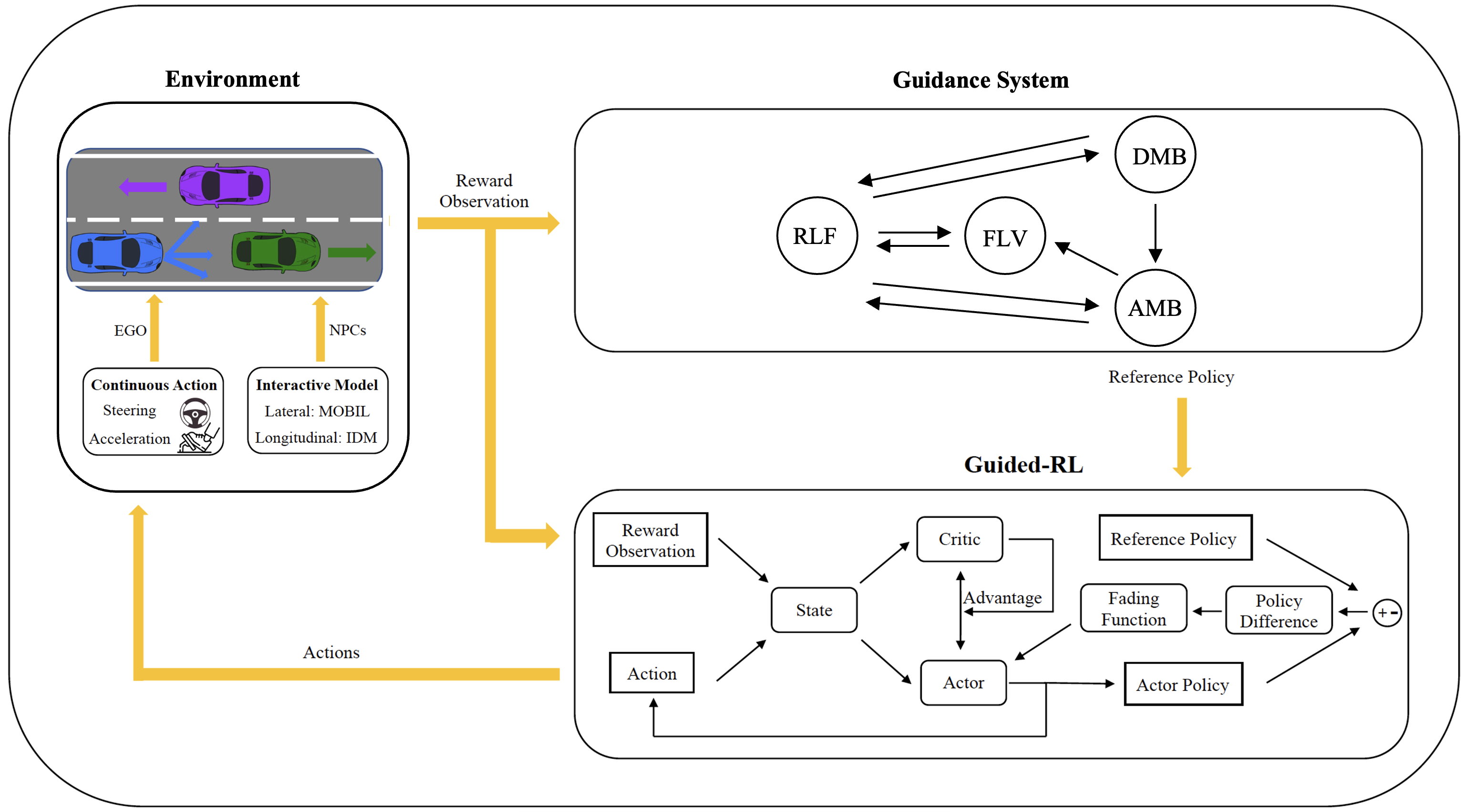
Figure 1: An illustration of the integrated DRL and expert system guidance framework. Initial training is heavily influenced by the guidance system, such as the constrained iterative LQR and PID controllers, with the fading guidance function progressively diminishing this expert influence over time.

A guidance system processes these observations and generates a reference policy, which serves as input for the guided Reinforcement Learning (RL) module. The RL agent employs this reference policy, along with information from the highway environment, to guide the optimization of its Critic and Actor networks, thus promoting efficient learning. Furthermore, a fading function is incorporated to progressively reduce the influence of guidance, enabling the RL agent to learn rapidly in the correct direction initially, and ultimately surpass the guidance it receives. Upon completing the training, the agent no longer relies on the guidance system to execute its policy within the environment. In essence, the framework functions in three primary phases:

• Observation Processing: A guidance system processes the information from the simulator and generates a reference policy. This policy provides the initial direction for the reinforcement learning agent.

• Guided Learning: The RL agent uses the reference policy and the highway environment information to optimize its neural networks (e.g. actor/critic). This process is guided by a fading function that gradually reduces the influence of the guidance, thus enabling the RL agent to learn rapidly in the right direction initially and eventually surpass the guidance it receives.

• Policy Execution: After the training phase, the RL agent executes its policy within the highway environment, independently of the guidance system.

Subsequent subsections provide an in-depth explanation of each component in the framework, including the Environment, Guidance System, and Reinforcement Learning with Fading Guidance.

III-A Environment

III-A1 Vehicle Kinematics Model

The kinematic bicycle model [25] is used to simulate the motion of the ego vehicle, which is the primary vehicle under the control of the autonomous driving algorithm being studied. This model adeptly captures the critical aspects of the vehicle’s movement, striking a balance between simplicity and computational efficiency.

III-A2 Non-Player Character Behaviours

We simulate other vehicles (non-player characters/NPCs) using Intelligent Driver Model (IDM) [26] for longitudinal motion and Minimizing verall Braking Induced by Lane change (MOBIL) model [27] for lateral motion. Inspired by [28, 29], four classes of NPC behavior are simulated (timid, normal, agressive, truck), each with different IDM/MOBIL parameters, as shown in Table I.

TABLE I: Parameters of Different Driving Types

Driver	Desired	Desired	Jam	Max	Desired	Politeness	Safe	Acceleration	Length	Width
types	speed	time	distance	acceleration	deceleration		braking	threshold
	(m/s)	(s)	(m)	(m/s2)	(m/s2)		(m/s2)	(m/s2)	(m)	(m)
Timid	27.8	2.0	4.0	0.8	-1.0	1.0	1.0	0.2	5	2
Normal	33.3	1.5	2.0	1.4	-2.0	0.5	2.0	0.1	5	2
Aggressive	38.9	1.0	0.0	2.0	-3.0	0.0	3.0	0.0	5	2
Truck	23.6	2.0	4.0	0.7	-2.0	1.0	1.0	0.2	6	2.5

III-A3 Observations

We assume that the ego vehicle is able to observe the positions, headings, and velocities of other nearby vehicles. The observation is represented as an $M\times 6$ matrix where each row encapsulates the kinematic data for the $M^{th}$ closest neighboring vehicle surrounding the ego vehicle (including the ego vehicle itself). This data can be represented as follows:

$$o_{i}=(p_{i},x_{i},y_{i},v_{i}^{x},v_{i}^{y},h_{i})_{i\in[0,M]}$$ (1)

In the above equation, $o_{i}$ signifies the $i^{th}$ row of the observation array. $p_{i}$ is a boolean variable that indicates the existence of the $i^{th}$ nearest neighbor vehicle. When $p_{i}$ is zero, all elements within $o_{i}$ are set to zero instead of removing the entire row from the observation array. This approach is crucial as it ensures a consistent size for the input layer, a requirement for neural networks. The variables $x_{i},y_{i},v_{i}^{x},v_{i}^{y},h_{i}$ denote the two-dimensional position, velocity, and heading angle, respectively, of the $i^{th}$ closest neighbor vehicle, as represented in the global coordinate system.

III-A4 Actions

Continuous actions corresponding to acceleration $\alpha$ and steering angle $\delta$ are used to directly set the low-level controls of the vehicle kinematics.

III-A5 Reward Function

We define the ego vehicle’s desired behavior using the reward function:

$$R= \;c_{1}R_{collision}+c_{2}R_{velocity}+c_{3}R_{steering}$$ (2)

$$+c_{4}R_{acceleration}+c_{5}R_{prize}$$

where negative rewards $R_{collision}$ are assigned when collisions occur with other vehicles or the ego vehicle crosses highway boundaries. To enhance traffic efficiency and minimize accident risk, a positive reward $R_{velocity}$ is introduced, proportional to the ego vehicle’s speed, within the range of maximum and minimum permissible speeds. In an effort to diminish jittering and enhance passenger comfort, a slight penalty $R_{steering}$ is imposed based on the steering angle. A minimal penalty $R_{acceleration}$ is applied in relation to acceleration to promote fuel efficiency. Upon successful arrival at the destination, the agent is granted a substantial reward $R_{prize}$. $\{c_{1},...,c_{5}\}$ represent the weights assigned to the agent’s safety, efficiency, passenger comfort, and task completion.

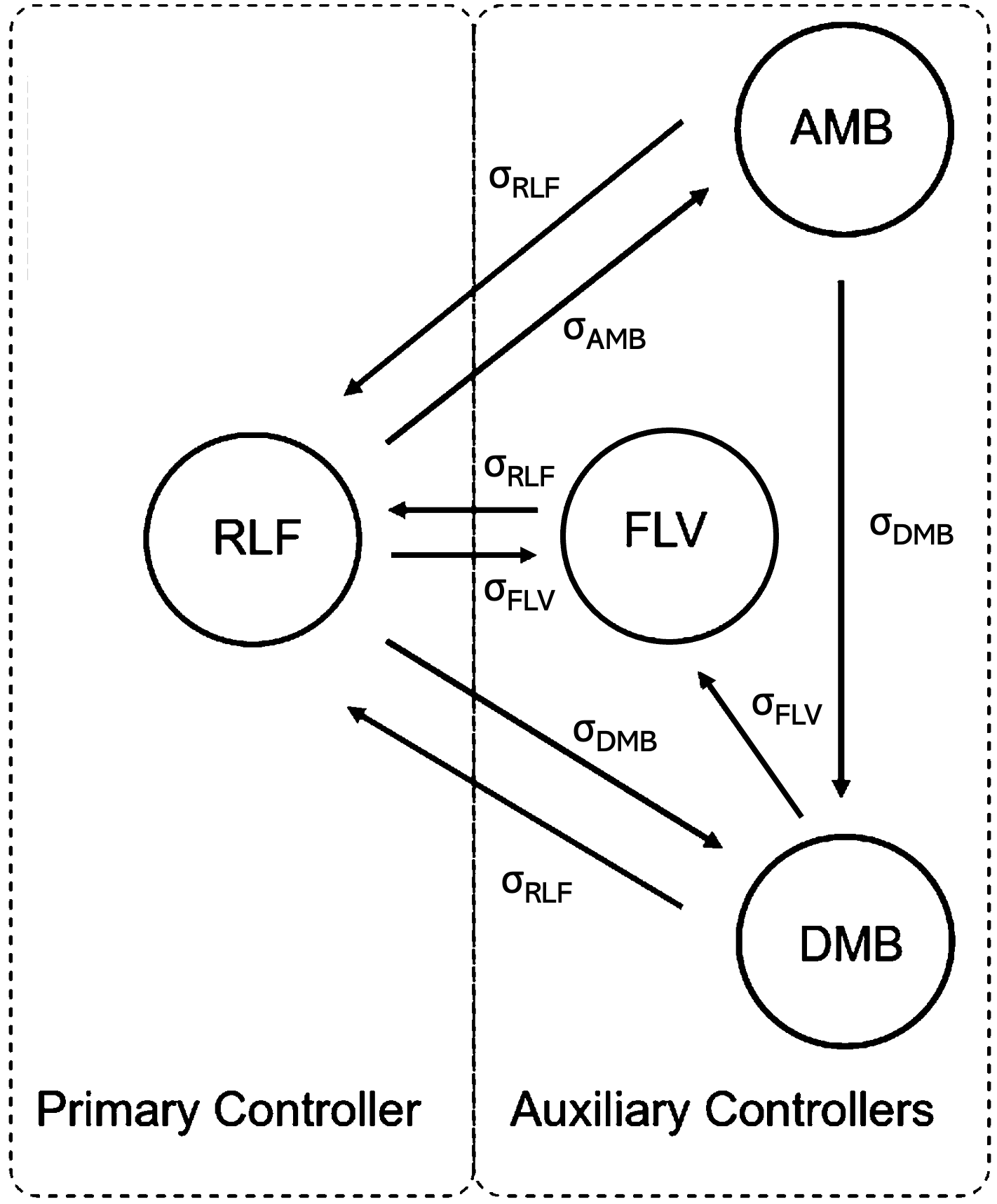
Figure 2: FSMs schematic for the proposed guidance system.

III-B Guidance System

The Guidance System in our framework denotes an expert driver controlled by either a data-driven policy, an optimal control method, or a human demonstrator. For this work, we have designed the Guidance System to act as a high-level decision-maker that operates the ego vehicle within a hierarchical structure. This involves a Finite State Machine which is a computational model used to represent and control the behavior of a system. It consists of a set of states, transitions, and actions. The Guidance System operates by initially identifying the necessary behavior for the controller based on predetermined rules, subsequently activating the corresponding controller, and relaying the requisite parameters.

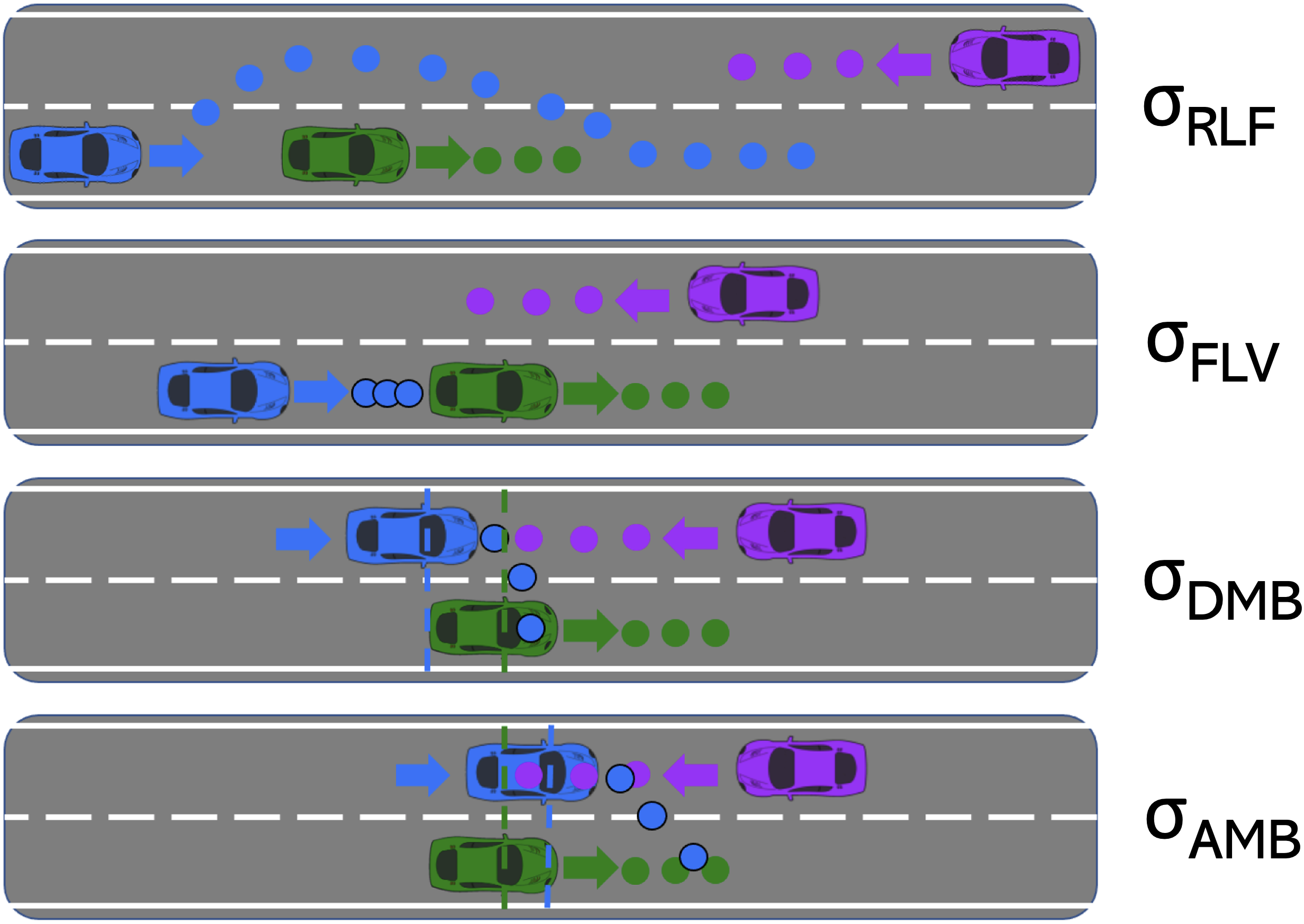
Figure 3: Transition conditions for Decision Making.

In order to accommodate the diverse range of maneuvers required by autonomous vehicles, we have incorporated four motion primitives, grouped into primary and auxiliary categories. The primary controller is represented by Responsive Lane Follow (RLF), while the auxiliary controllers consist of Follow Leading Vehicle (FLV), Decelerate and Merge Back (DMB), and Accelerate and Merge Back (AMB). Brief descriptions of these states are provided as follows:

• RLF: In this state, the ego vehicle is instructed to adhere to its assigned trajectory and to commence an overtaking maneuver upon detecting another vehicle. The RLF state is primarily aimed at executing obstacle-free trajectory optimization, and it’s expected that the vehicle will transition into this state whenever feasible.

• FLV: In this state, the ego vehicle is instructed to maintain a specific distance behind the leading vehicle.

• DMB: During an overtaking maneuver, the ego vehicle is directed to abandon the action if needed. This is done by reducing the speed at a prescribed deceleration rate and rejoining the original lane, provided it is free of any NPC.

• AMB: In the midst of overtaking, the ego vehicle is prompted to expedite the process by accelerating at a given rate and merging back into the lane once it is confirmed to be free of any NPC.

The transitions between those states are triggered as follows:

• $\sigma_{RLF}$: When trajectories planned by RLF do not intersect with either other vehicles or road boundaries.

• $\sigma_{FLV}$: When $\sigma_{RLF}$ is False and the ego vehicle is not on the opposite lane.

• $\sigma_{DMB}$: When $\sigma_{RLF}$ is False and the ego vehicle is on the opposite lane with its center point behind the leading vehicle.

• $\sigma_{AMB}$: When $\sigma_{RLF}$ is False and the ego vehicle is on the opposite lane with its center point crossing the leading vehicle.

Figures 2 and 3 provide illustrations of the states and their transition conditions. The implementation of the primary and auxiliary controllers is outlined as follows:

III-B1 Primary Controller

Responsive Lane Follow is considered to be the primary controller and is implemented as a trajectory optimization that solves the following constrained optimal control problem:

$$\underset{u_{0},...,u_{N-1}}{\text{min}} \ell^{f}(s_{N})+\sum_{k=0}^{N-1}\ell(s_{k},u_{k})$$ (3)

subject to $$s_{k+1}=f(s_{k},u_{k}),\quad k=0,...,N-1$$

$$g(s_{k},u_{k})<0,\;\;\quad\quad k=0,...,N-1$$

$$g(s_{N})<0$$

given $$s_{0}=s_{init}$$

where $s_{k}$ and $u_{k}$ are the state vector and the control input vector at time step $k$, respectively. $N$ is the total number of discrete steps through the horizon of the trajectory. $\ell^{f}(\cdot)$ and $\ell(\cdot)$ are the final and stage cost functions. $f(\cdot)$ is the bicycle model [25] based transition dynamics of the ego vehicle. $g(\cdot)$ is the vector of constraints that defines obstacle avoidance and staying within the boundaries of the road.

In order to solve this problem in a computationally efficient way, we employed a Constrained Iterative Linear Quadratic Regulator (CiLQR) algorithm. A typical iLQR algorithm is used to solve the problem posed in (3) without the constraints $g(\cdot)$ by employing forward and backward passes iteratively.

To address constraints in such methods, in this study, we have chosen the penalty barrier method with exponential barrier function due to its computational efficiency and proved convergence property [15]. The method is suitable for a wide range of problems and can be effective when a proper differentiable barrier function is employed. The fundamental concept is to utilize a barrier function to shape the constraint functions:

$$c(s,)=b(g(s,u))$$ (4)

Subsequently, the objective function is augmented with the barrier function. The optimal barrier function is the indicator function:

$$b^{*}(g(s,u))=\begin{cases}\infty,g(s,u)\geq 0\\ 0,g(s,u)<0\end{cases}$$ (5)

The indicator function has the ability to represent the original constraints. Nonetheless, as the indicator function is not differentiable, the majority of numerical optimization methods cannot optimize the augmented objective function. As a result, it is necessary to identify a differentiable barrier function that can approximate the indicator function as:

$$b(g(s,u))=q_{1}exp(q_{2}g(s,u))$$ (6)

where $q1,q_{2}$ and $t>0$ are parameters.

Once the constraints are augmented to the cost through barrier function, CiLQR algorithm is implemented through iterations between forward and backward passes until the convergence achieved. For the first iteration, a feasible initial trajectory is designated as the nominal trajectory $\bar{s},\bar{u}$.

Backward Pass linearizes the system dynamics around the current trajectory, and approximates the cost function ($Q^{k}(s_{k},u_{k})$) as quadratic:

$$Q^{k}(\delta s_{k},\delta u_{k})\\ \approx\frac{1}{2}\begin{bmatrix}1\\ \delta s_{k}\\ \delta u_{k}\end{bmatrix}^{\top}\begin{bmatrix}0&(Q_{s}^{k})^{\top}&(Q_{u}^{k})^{\top}\\ Q_{s}^{k}&Q_{ss}^{k}&Q_{su}^{k}\\ Q_{u}^{k}&Q_{us}^{k}&Q_{uu}^{k}\end{bmatrix}\begin{bmatrix}1\\ \delta s_{k}\\ \delta u_{k}\end{bmatrix}$$ (7)

$$Q^{k}_{s} =L^{k}_{s}+(f^{k}_{s})^{\top}V^{k+1}_{s}$$ (8)

$$Q^{k}_{u} =L^{k}_{u}+(f^{k}_{u})^{\top}V_{s}^{k+1}$$

$$Q^{k}_{ss} =L^{k}_{ss}+(f^{k}_{s})^{\top}V^{k+1}_{ss}f^{k}_{s}+V^{k+1}_{s}f^{k}_{ss}$$

$$Q^{k}_{uu} =L^{k}_{uu}+(f^{k}_{u})^{\top}V^{k+1}_{ss}f^{k}_{s}+V^{k+1}_{s}f^{k}_{uu}$$

$$Q^{k}_{us} =L^{k}_{us}+(f^{k}_{u})^{\top}V^{k+1}_{ss}f^{k}_{s}+V^{k+1}_{s}f^{k}_{us}$$

In the above expression, $L(\cdot)$ represents the cost function augmented with the barrier functions corresponding to constraints. The subscripts in equation (8) indicate either the first or the second derivatives of the function with respect to the variable they annotate. Meanwhile, $V^{k+1}(\cdot)$ denotes the value function for the subsequent iteration ($k+1$). The optimal control at each step is then determined as:

$$\delta u_{k}^{*}=-(Q^{k}_{uu})^{-1}(Q_{u}^{k}+Q^{k}_{us}\delta s_{k})$$ (9)

By plugging this optimal control in the approximated action value function, the derivatives of the value function at time $k$ can be calculated as:

$$V_{s}^{k} =Q_{s}^{k}-Q_{u}^{k}(Q_{uu}^{k})^{-1}Q_{us}^{k}$$ (10)

$$V^{k}_{ss} =Q^{k}_{ss}-Q^{k}_{su}(Q^{k}_{uu})^{-1}Q^{k}_{us}$$

Since $V^{N}(\cdot)$ equals to $\ell^{f}(\cdot)$, optimal control policy given in (9) can be calculated at each step starting from $N$ to 0.

Forward Pass simulates the dynamics forward once the backward pass is completed, by using the optimal control starting from 0 to $N$ as:

$$s_{0} =s_{init}$$ (11)

$$u_{k} =\bar{u}_{k}+q_{k}-(Q^{k}_{uu})^{-1}(Q_{u}^{k}+Q^{k}_{us}\delta s_{k})$$

$$s_{k+1} =f(s_{k},u_{k})$$

Upon the completion of forward pass, the nominal trajectory $(\bar{s},\bar{u})$ will be replaced by the improved new actual trajectory $(s,u)$, resulting in enhanced performance. These steps repeatedly follow each other, until the convergence is achieved. Details regarding implementation and regularizations can be found in [15, 30].

III-B2 Auxiliary Controllers

While the primary controller efficiently manages obstacle-free trajectory planning, it lacks the capability to deal with exceptional scenarios, particularly the need to abort an overtaking maneuver. To remedy this, we have introduced three additional motion primitives as auxiliary controllers (FLV, DMB, and AMB). These controllers, detailed at the start of this section, aid in addressing these unique situations, thereby providing a more comprehensive control strategy and were implemented as classical PID controllers as follows:

$$u=K_{p}e+K_{i}\int edt+K_{d}\frac{de}{dt}$$ (12)

where $K_{p}$, $K_{i}$, and $K_{d}$ are the proportional, integral, and derivative gains, respectively. $e$ is the error defined individually for acceleration and steering inputs in each Auxiliary Controllers.

In FLV, the acceleration error is derived from the spatial discrepancy between the ego vehicle and the leading vehicle. Concurrently, the steering error corresponds to the extent of deviation from the median of the occupied lane. In DMB, the acceleration controller generates a predetermined deceleration rate until the leading NPC is fully surpassed. Subsequent to this event, the error term for the steering controller is determined by the distance from the mid-line of the original lane. Conversely, in AMB, the acceleration controller issues a prescribed acceleration rate until the ego vehicle has completely overtaken the leading NPC. Following this overtaking, the error term for the steering controller is computed based on the distance from the center line of the initial lane.

III-C Reinforcement Learning with Fading Guidance

Reinforcement Learning (RL) is a type of machine learning where an agent learns to make decisions by interacting with an environment. It can be formally defined by a tuple $(S,A,P,r,\gamma)$ representing the state space $S$, the action space $A$, the state transition probability $P$, the reward function $R$, and the discount factor $\gamma$. An agent learns from the environment by observing the state $s\in S$, taking an action $a\in A$, and receiving a reward $r(s,a)$.

An optimal value function $Q^{*}:S\times A\rightarrow\mathbb{R}$ describes the expected cumulative rewards when starting from a given state and following the best policy. The goal of the agent is to learn the optimal policy

$$\pi^{*}(s)=\underset{a}{\operatorname{argmax}}Q^{*}(s,a)$$ (13)

that corresponds to the optimal value function

$$Q^{*}(s,a)=\max_{\pi}\mathbb{E}\left(\sum_{t=0}\gamma^{t}r\left(s_{t},a_{t}\right)\mid s_{0}=0,a_{0}=a\right).$$ (14)

In our framework, policy from the guidance system guides the RL agent during training, and a fading function is also introduced to fade the guidance effect gradually, which enables the agent to learn in the right direction fast at the beginning and learn beyond the guidance in the end.

The RL agent receives a reference policy from the guidance system, which steers the update of the Actor Networks using the loss function:

$$L_{guidance}=\delta(\pi_{actor}(s),\pi_{reference}(s))$$ (15)

where $L_{guidance}$ represents the guidance loss, while $\delta$ can be any function representing the divergence between its inputs. In our study, we adopt the Mean Squared Error to define $\delta$.

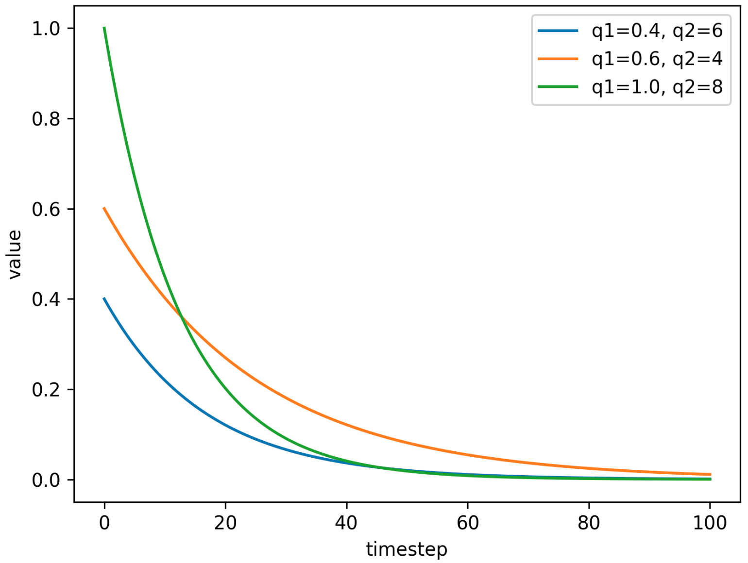
Figure 4: Effect of $q_{1}$, $q_{2}$ parameters on the shape of fading functions.

Fading functions, which regulate the amount of guidance during training, can be any function that decreases over time, and its diminishing rate can be parameterized. Here, we employed the inverse of an exponential function as:

$$\beta(t)=\frac{q_{1}}{exp(q_{2}t/T)}$$ (16)

where $T$ is the total number of timesteps, which has a normalization effect, $t$ is the timestep optimizers currently performing the update, and $q_{1}$, $q_{2}$ are parameters that modify the shape of the fading curve (Figure 4).

Lastly, the actor loss function that the optimizer intends to minimize is

$$L_{actor}=L_{policy}+\beta(t)L_{guidance}$$ (17)

where $L_{policy}$ is the policy loss of the specific RL algorithm. Once the training is completed, the guidance system is no longer needed for the agent to execute the trained policy in the environment.

IV Experimental Results

IV-A Simulation

An open-source autonomous driving simulation framework [31] is adapted and customized for the purpose of this research. Our highway environment is characterized by a road length of 1000 m, divided into two lanes. Vehicles in these lanes travel in opposing directions, with each lane having a width of 4 m. The ego vehicle starts with an initial velocity of 45 m/s, has a maximum speed of 60 m/s, and measures 2 m in width and 5 m in length. Its maximum permissible acceleration and steering are 5.5 m/s² and 1.0 radian, respectively. The simulation operates at a frequency of 100 Hz and can run for a maximum of 5,000 timesteps per episode. Episodes conclude upon a collision, once the destination is reached, or if the episode’s duration exceeds the set threshold. In terms of traffic, the driving types distribution mirrors real-world scenarios with 60$\%$ normal, 20$\%$ timid, 10$\%$ aggressive, and 10$\%$ being trucks [28, 29]. Forward-driving vehicles are spaced 80 m apart, while vehicles in opposite lanes have 180 m intervals, with random noise added to their base positions. Unlike previous studies, such as [16], which only considered vehicle-to-vehicle collisions, our environment also accounts for collisions between the ego vehicle and road boundaries, enhancing realism.

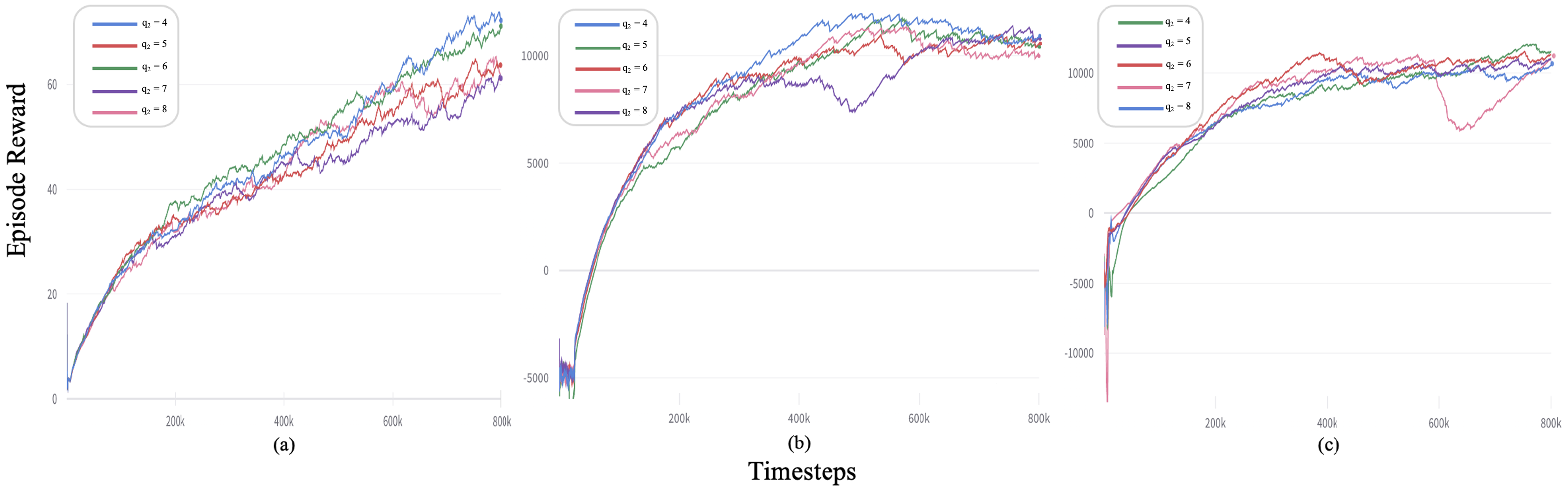
Figure 5: Effect of fading functions with different $q_{2}$ parameters on training performance of the (a) G-PPO, (b) G-TD3, (c) G-SAC algorithms.

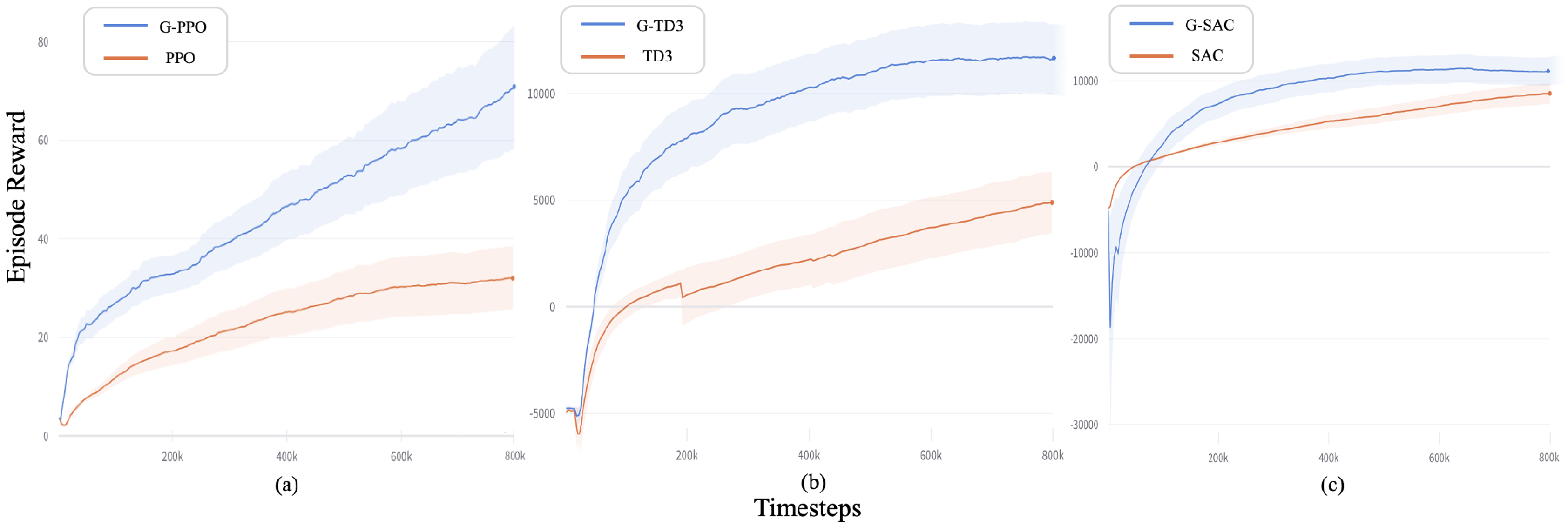
Figure 6: Training performance of the three algorithms with and without guidance (average over 5 random seeds).

IV-B Training

We utilized three state-of-the-art algorithms for continuous environments as baselines to validate our method: Proximal Policy Optimization (PPO) [32], Twin Delayed DDPG (TD3) [33], and Soft Actor-Critic (SAC) [34]. Within our guided RL framework, these are respectively referred to as G-PPO, G-TD3 and G-SAC.

The training spanned 800 thousand timesteps with reward parameters set as $c_{1}$=$-10,c_{2}$=$1,c_{3}$=$c_{4}$=$1$, and $c_{5}$=$100$. These parameters prioritize reaching the destination as soon as possible, avoiding collisions, and maximizing energy efficiency and stability. From our preliminary experiments, we found the most effective normalization settings to be:

• PPO: Both rewards and observations are normalized.

• TD3: Only observations are normalized.

• SAC: Neither rewards nor observations are normalized.

We first analyzed the impact of various fading functions on training performance. The scaling factor $q_{1}$ ensures policy and guidance losses are comparable, while $q_{2}$ modulates the guidance effect’s diminishing rate. Figure 5 reveals that guided algorithms remain robust for $q_{2}$ values between four and eight. Notably, G-TD3 with $q_{2}=8$ and G-SAC with $q_{2}=7$ experience temporary declines but recover to surpass ten thousand episode rewards by training’s end. A smaller $q_{2}$ appears to enhance training stability by ensuring a gentler fade of the guidance effect.

Upon determining optimal fading functions, we delved into the guidance’s enhancement on baseline algorithms. For subsequent experiments, $q_{1}$ was adjusted to match the initial guidance and policy loss magnitudes, and all $q_{2}$ values were set to 4 for consistent fading and stability. Results were averaged across five random seeds.

Figure 6 underscores guidance’s significant enhancement of the baseline algorithms’ sample efficiency:

• PPO: PPO converges slower than its counterparts. By training’s end, while the baseline tends to stabilize, the G-PPO continues its ascent. Here, guidance acts as a potent exploration tool, preventing the RL agent from settling at undesired local minima.

• TD3: The G-TD3 converges over 200 thousand timesteps earlier. The baseline reaches only half the episode reward of its guided counterpart. Both exhibit a learning rate shift around 200 thousand timesteps, but the G-TD3 transitions more smoothly.

• SAC: Despite initial setbacks, the G-SAC surpasses its baseline before 100 thousand timesteps. Among the three, SAC converges the fastest. Yet, G-SAC further accelerates this, achieving rewards in a quarter of the time taken by its baseline.

TABLE II: Evaluation Result of Baselines and Guided Algorithms (best results are bolded)

Evaluation Metrics	Guidance System	PPO	G-PPO	TD3	G-TD3	SAC	G-SAC
Episode reward	5940.9	5437.31	6421.85	3462.42	6702.52	100112.66	14879.58
Speed (m/s)	42,97	40.1	44.76	45.85	45.19	59.64	57.2
Displacement (m)	440.26	350.29	466.68	356.76	451.07	638.42	807.73
Computation time (ms)	74	0.1	0.33	0.82	0.27	0.89	0.86
Energy consumption	1.21	0.34	1.39	2.45	0.98	1.36	0.52
Vehicles collision rate	1	1	1	0.2	0.8	0.7	0.3
Boundaries collision rate	0	0	0	0.8	0	0.1	0.2

IV-C Evaluation

In this section, we evaluate the guidance system, baseline RL algorithms, and their guided versions. Given the random noise introduced during training for exploration, all algorithms are anticipated to exhibit enhanced performance during the evaluation phase without action noise.

Beyond the primary metric of rewards, we also dissect the components constituting the overall reward. This granular approach aids in discerning which specific elements the algorithm prioritizes for optimization. Results represent averages over 5 random seeds, with 10 episodes per seed. For a direct comparison during evaluation, rewards remain unnormalized. The findings are detailed in Figure 7 and Table II.

The evaluation metrics include:

• Reward: Cumulative reward per episode.

• Speed (m/s): Ego vehicle’s average speed per timestep.

• Displacement (m): Average distance the ego vehicle covers within each episode before termination.

• Computation time (ms): Average duration required for the agent to determine an action pair from an observation.

• Energy consumption: Represented by the average absolute acceleration per timestep. Longer episodes typically consume more energy, making per-timestep averages more comparable.

• Vehicles collision rate: Average likelihood of the ego vehicle colliding with other vehicles.

• Boundaries collision rate: Average likelihood of the ego vehicle colliding with road boundaries.

Our experimental results affirm the superior performance of guided algorithms over their baselines, particularly in terms of average episode reward—a trend consistent with training outcomes. Guided algorithms consistently achieve higher rewards and displacements, consuming roughly the same computation time. Notably, G-PPO prioritizes speed optimization, while G-TD3 and G-SAC emphasize energy efficiency.

Both G-SAC and G-TD3 agents surpass the guidance system across all evaluation metrics. Remarkably, agents compute actions over eight times faster, reaching destinations quicker and more energy-efficiently. Instead of manually designing finite state machines to address expert system failures, it’s more pragmatic to let the RL agent learn beyond the expert system, aided by a fading guidance function. Experiments validate that as guidance influence diminishes, our algorithm can indeed learn beyond the guidance system.

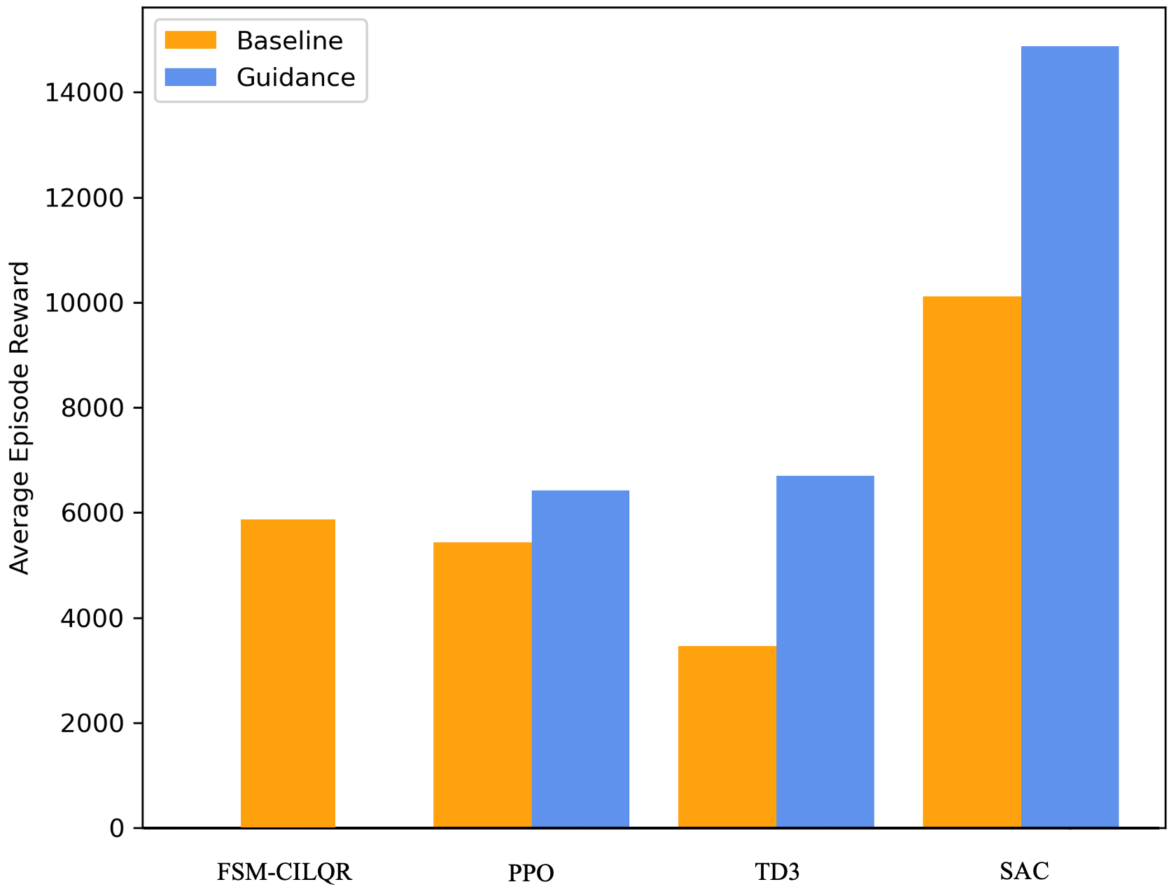
Figure 7: Average episode reward of baselines and guided algorithms.

V Conclusion

In this study, we have presented a new integration of expert system guidance with deep reinforcement learning to address the complex challenge of autonomous overtaking in highway settings. By leveraging the strengths of both rule-based and learning-based approaches, our framework introduces a fading guidance mechanism, enabling the DRL agent to benefit from expert direction during initial stages of training while subsequently expanding its capabilities beyond those of the expert system. Our evaluations indicate significant improvements in sample efficiency, driving performance, and safety compared to baseline DRL algorithms. As the realm of autonomous driving continually evolves, the power of combined expertise and adaptability offers a promising direction.

Declaration of Conflicting Interests

This article’s author(s) reported no potential conflicts of interest in relation to its research, authorship, or publication.

Jinxiong Lu received his B.Sc. in Mechanical Engineering from Jilin University, China in 2021. He is currently working toward the M.Sc. degree with the department of Electrical Engineering at Aalto University, Finland. His research focuses on Optimal Control and Reinforcement Learning.

Gokhan Alcan received his M.Sc. and Ph.D. degrees in Mechatronics Engineering from Sabanci University, Istanbul, Turkey in 2015 and 2019, respectively. In 2019, he was a postdoctoral researcher in the Control, Vision, and Robotics Research Group at Sabanci University before joining Aalto University. Since 2020, he has been a postdoctoral researcher in the Intelligent Robotics Research Group at Aalto University. His primary research interests are safe model predictive control, constrained optimal control theory, system identification/machine learning, and their applications to dynamical systems and autonomous driving.

Ville Kyrki (M’03–SM’13) received the M.Sc. and Ph.D. degrees in computer science from Lappeenranta University of Technology, Lappeenranta, Finland, in 1999 and 2002, respectively. In 2003-2004, he was a Postdoctoral Fellow with the Royal Institute of Technology, Stockholm, Sweden, after which he returned to Lappeenranta University of Technology, holding various positions in 2003-2009. During 2009-2012, he was a Professor of computer science, Lappeenranta University of Technology. Since 2012, he is currently an Associate Professor of Intelligent Mobile Machines with Aalto University, Helsinki, Finland. His primary research interests include robotic perception, decision making, and learning. Dr. Kyrki is a Fellow of Academy of Engineering Sciences (Finland), and a member of Finnish Robotics Society and Finnish Society of Automation. He was a Chair and Vice Chair of the IEEE Finland Section Jt. Chapter of CS, RA, and SMC Societies in 2012-2015 and 2015-2016, respectively, Treasurer of IEEE Finland Section in 2012-2013, and Co-Chair of IEEE RAS TC in Computer and Robot Vision in 2009-2013. He was an Associate Editor for the IEEE Transactions on Robotics in 2014-2017.

References

- [1] J. Palatti, A. Aksjonov, G. Alcan, V. Kyrki, ”Planning for safe abortable overtaking maneuvers in autonomous driving.” in IEEE International Intelligent Transportation Systems Conference, 508–514, 2021.
- [2] X. Tang, B. Huang, T. Liu and X. Lin, ”Highway Decision-Making and Motion Planning for Autonomous Driving via Soft Actor-Critic,” in IEEE Transactions on Vehicular Technology, 71, 5, 4706–4717, 2022.
- [3] M. Xiaoqiang, Y. Fan, L. Xueyuan, L. Qi, G. Xin and L. Zirui, ”Graph Convolution Reinforcement Learning for Decision-Making in Highway Overtaking Scenario,” IEEE Conference on Industrial Electronics and Applications, 417–422, 2022.
- [4] Y. Kim, D.S. Pae, S.H. Jang, S.W. Kang and M.T. Lim, ”Reinforcement Learning for Autonomous Vehicle using MPC in Highway Situation.” in IEEE International Conference on Electronics, Information, and Communication 1–4, 2022.
- [5] A. Aksjonov and V. Kyrki, ”A Safety-Critical Decision-Making and Control Framework Combining Machine-Learning-Based and Rule-Based Algorithms,” SAE International Journal on Vehicle Dynamics, Stability and NVH, 7(3), 2023.
- [6] Q. Wu, S. Cheng, L. Li, F. Yang, L.J. Meng, Z.X. Fan, H.W. Liang, ”A fuzzy-inference-based reinforcement learning method of overtaking decision making for automated vehicles.” Journal of Automobile Engineering, 236, 1, 75–83, 2022.
- [7] S.H. Bae, S.H. Joo, J.W. Pyo, J.S. Yoon, K. Lee, T.Y. Kuc, ”Finite state machine based vehicle system for autonomous driving in urban environments.” in International Conference on Control, Automation and Systems, 1181–1186, 2020.
- [8] M. Zhang, N. Li, A. Girard, I. Kolmanovsky, ”A finite state machine based automated driving controller and its stochastic optimization.” in Dynamic Systems and Control Conference, 2017.
- [9] J. Chen, C. Liu, M. Tomizuka, ”Foad: Fast optimization-based autonomous driving motion planner.” in IEEE American Control Conference, 4725-4732, 2018.
- [10] J. Zhang, ”C-B’ezier curves and surfaces.” Graphical Models and Image Processing, 61, 1999.
- [11] S. Luo, X. Li, Z. Sun, ”An optimization-based motion planning method for autonomous driving vehicle.” in International Conference on Unmanned Systems, 739–744, 2020.
- [12] E.F. Camacho, C. Bordons, E.F. Camacho, C. Bordons, ”Model Predictive Controllers.” Springer, 2007.
- [13] G. Cesari, G. Schildbach, A. Carvalho, F. Borrelli, ”Scenario model predictive control for lane change assistance and autonomous driving on highways.” IEEE Intelligent transportation systems magazine, 9, 3, 2017.
- [14] A. Bemporad, M. Morari, V. Dua, E.N. Pistikopoulos, ”The explicit linear quadratic regulator for constrained systems.”, Automatica, 38, 1, 2002.
- [15] J. Chen, W. Zhan, M. Tomizuka, ”Autonomous driving motion planning with constrained iterative LQR.” IEEE Transactions on Intelligent Vehicles, 4, 2, 2019.
- [16] F. Ye, X. Cheng, P. Wang, C.Y. Chan, J. Zhang, ”Automated lane change strategy using proximal policy optimization-based deep reinforcement learning.” in IEEE Intelligent Vehicles Symposium, 1746–1752, 2020.
- [17] P. Wolf, K. Kurzer, T. Wingert, F. Kuhnt, J.M. Zollner, ”Adaptive behavior generation for autonomous driving using deep reinforcement learning with compact semantic states.” in IEEE Intelligent Vehicles Symposium, 993–1000, 2018.
- [18] S. Chakraborty, S. Kumar, N. Bhatt, R. Pasumarthy, ”End-to-end Autonomous Driving in Heterogeneous Traffic Scenario Using Deep Reinforcement Learning.” in European Control Conference, 1–6, 2023.
- [19] C. Xu, W. Zhao, J. Liu, C. Wang, C. Lv, ”An Integrated Decision-Making Framework for Highway Autonomous Driving Using Combined Learning and Rule-Based Algorithm.”, IEEE Transactions on Vehicular Technology, 71, 4, 2022.
- [20] S. Mo, X. Pei, Z. Chen, ”Decision-making for oncoming traffic overtaking scenario using double DQN.”, IEEE Conference on Vehicle Control and Intelligence, 1–4, 2019.
- [21] Y. Kim, D.S. Pae, S.H. Jang, S.W. Kang, M.T. Lim, ”Reinforcement Learning for Autonomous Vehicle using MPC in Highway Situation.” in International Conference on Electronics, Information, and Communication, 1–4, 2022.
- [22] J. Rong, N. Luan, ”Safe reinforcement learning with policy-guided planning for autonomous driving.” in IEEE International Conference on Mechatronics and Automation, 320–326, 2020.
- [23] L. Wang, J. Liu, H. Shao, W. Wang, R. Chen, Y. Liu, S.L. Waslander, ”Efficient Reinforcement Learning for Autonomous Driving with Parameterized Skills and Priors.” arXiv:2305.04412 , 2023.
- [24] H. Chen, Y. Zhang, U.A. Bhatti, M. Huang, ”Safe Decision Controller for Autonomous Driving Based on Deep Reinforcement Learning in Nondeterministic Environment.” Sensors, 23, 3, 2023.
- [25] P. Polack, F. Altché, B. d’Andréa-Novel, A de La Fortelle, ”The kinematic bicycle model: A consistent model for planning feasible trajectories for autonomous vehicles?.” in IEEE intelligent vehicles symposium, 812–818, 2017.
- [26] J. Kong, M. Pfeiffer, G. Schildbach, F. Borrelli, ”Kinematic and dynamic vehicle models for autonomous driving control design.” In 2015 IEEE intelligent vehicles symposium, 1094–1099, 2015.
- [27] A. Kesting, M. Treiber, D. Helbing, ”General lane-changing model mobil for car-following models,” Transportation Research Record, 1999, 1, 86-–94, 2007.
- [28] Z.N. Sunberg, Safety and efficiency in autonomous vehicles through planning with uncertainty, 2018.
- [29] A. Kesting, M. Treiber, D. Helbing, ”Agents for traffic simulation.” Multi-agent systems: Simulation and applications, 5, 2009.
- [30] G. Alcan, V. Kyrki, ”Differential dynamic programming with nonlinear safety constraints under system uncertainties.” IEEE Robotics and Automation Letters, 7(2), 1760-1767, 2022.
- [31] E. Leurent, ”An environment for autonomous driving decision-making”, GitHub repository, 2018.
- [32] J. Schulman, F. Wolski, P. Dhariwal, A. Radford, O. Klimov, ”Proximal policy optimization algorithms.” arXiv:1707.06347, 2017.
- [33] S. Dankwa, W. Zheng, ”Twin-delayed ddpg: A deep reinforcement learning technique to model a continuous movement of an intelligent robot agent.” in Proceedings of the 3rd international conference on vision, image and signal processing, 1–5, 2019.
- [34] T. Haarnoja, A. Zhou, P. Abbeel, S. Levine, ”Soft actor-critic: Off-policy maximum entropy deep reinforcement learning with a stochastic actor.” in International conference on machine learning, 1861–1870, 2018.