Towards Understanding the Generalizability of Delayed Stochastic Gradient Descent

Abstract

Stochastic gradient descent (SGD) performed in an asynchronous manner plays a crucial role in training large-scale machine learning models. However, the generalization performance of asynchronous delayed SGD, which is an essential metric for assessing machine learning algorithms, has rarely been explored. Existing generalization error bounds are rather pessimistic and cannot reveal the correlation between asynchronous delays and generalization. In this paper, we investigate sharper generalization error bound for SGD with asynchronous delay $\tau$. Leveraging the generating function analysis tool, we first establish the average stability of the delayed gradient algorithm. Based on this algorithmic stability, we provide upper bounds on the generalization error of $\tilde{\mathcal{O}}(\frac{T-\tau}{n\tau})$ and $\tilde{\mathcal{O}}(\frac{1}{n})$ for quadratic convex and strongly convex problems, respectively, where $T$ refers to the iteration number and $n$ is the amount of training data. Our theoretical results indicate that asynchronous delays reduce the generalization error of the delayed SGD algorithm. Analogous analysis can be generalized to the random delay setting, and the experimental results validate our theoretical findings.

1 Introduction

First-order gradient-based optimization methods, such as stochastic gradient descent (SGD), are the mainstay of supervised machine learning (ML) training today (Robbins and Monro, 1951; Bottou et al., 2018). The plain SGD starts from an initial point $\mathbf{w}_{0}$ and trains iteratively on the training datasets by $\mathbf{w}_{t+1}=\mathbf{w}_{t}-\eta\mathbf{g}_{t}$, where $\mathbf{w}_{t}$ denotes the current iteration, $\eta$ is the learning rate, and $\mathbf{g}_{t}$ represents the gradient evaluated at $\mathbf{w}_{t}$. In practice, SGD not only learns convergent models efficiently on training datasets, but surprisingly, the learned solutions perform well on unknown testing data, exhibiting good generalization performance (Zhang et al., 2017; Du et al., 2019). Generalizability is a focal topic in the ML community, and there has been considerable effort to investigate the generalization performance of gradient-based optimization methods from the algorithmic stability perspective (Hardt et al., 2016; Kuzborskij and Lampert, 2018; Lei and Ying, 2020; Bassily et al., 2020; Zhang et al., 2022; Zhou et al., 2022).

However, in modern ML applications, the scale of samples in the training datasets and the number of parameters in the deep neural network models are so large that it is imperative to implement gradient methods in a distributed manner (Deng et al., 2009; Dean et al., 2012; Brown et al., 2020). Consider a distributed parameter server training system with $M$ workers and the distributed SGD performed as $\mathbf{w}_{t+1}=\mathbf{w}_{t}-\eta\sum_{m=1}^{M}\mathbf{g}_{t}^{m}/M$, where $\mathbf{g}_{t}^{m}$ represents the gradient evaluated by the $m$-th worker at the $t$-th iteration (Zinkevich et al., 2010; Li et al., 2014). This straightforward distributed implementation synchronizes the gradients from all workers at each iteration, which facilitates algorithmic convergence but imposes a significant synchronization overhead on the distributed training system (Assran et al., 2020).

An alternative approach to tackling this synchronization issue is employing asynchronous training, which eliminates the synchronization barrier and updates the model whenever the server receives gradient information without waiting for any other workers (Nedić et al., 2001; Agarwal and Duchi, 2011; Lian et al., 2015). It is essential to note that when the server receives the gradient data from a particular worker, the global model parameter has undergone several asynchronous updates, making asynchronous training a delayed gradient update. Hence the delayed SGD performs as $\mathbf{w}_{t+1}=\mathbf{w}_{t}-\eta\mathbf{g}_{t-\tau}$, where $\tau$ denotes the asynchronous delay and $\mathbf{g}_{t-\tau}$ is the gradient evaluated at $\mathbf{w}_{t-\tau}$ (as shown in Figure 2). Despite the existence of delayed updates, extensive theoretical work has been developed to guarantee the convergence of delayed gradient methods (Zhou et al., 2018; Arjevani et al., 2020; Stich and Karimireddy, 2020; Cohen et al., 2021; Mishchenko et al., 2022).

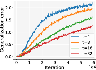
Figure 1: Generalization error of the ResNet-18 model trained with delayed SGD for classifying the CIFAR-100 data set. The experiment varied only the asynchronous delays and fixed other parameters, where the learning rate $\eta=0.1$.

While the convergence properties of delayed gradient methods have been widely studied, their generalization performance has yet to be explored, and generalization is the ultimate goal of the ML community. Regatti et al. (2019) analyzed the generalization performance of the delayed SGD algorithm in the non-convex case with the uniform stability framework, and gave an upper bound on the generalization error of $\mathcal{O}(T^{\tau}/n\tau)$, where $T$ is the iteration number and $n$ denotes the number of training samples. Although Regatti et al. claim that "distributed SGD generalizes well under asynchrony," their theoretical upper bound is rather pessimistic. Moreover, empirical evidence suggests that increasing the asynchronous delay reduces the generalization error at an appropriate learning rate, as illustrated in Figure 1, which cannot be explained by the results of (Regatti et al., 2019). Therefore, there is an imperative demand for a theoretical study into the inherent connection between asynchronous delay and generalization error for gradient descent algorithms.

This paper is devoted to understanding the effect of asynchronous delays on the generalization error of the delayed stochastic gradient descent algorithm. We focus on a convex quadratic optimization problem, which is a fundamental and critical topic in the ML community. Empirical evidence demonstrates that the local regions around the minimum of non-convex deep neural networks are usually convex (Li et al., 2018), and utilizing local quadratic approximations around the minimum is a fruitful way to study the behavior of deep neural networks (Jacot et al., 2018; Ma et al., 2018; He et al., 2019; Zou et al., 2021). In this study, we investigate the data-dependent average stability of delayed SGD to estimate the generalization error of the algorithm. Recursive sequences related to the algorithmic stability are established for the quadratic optimization problem. It is worth noting that the established recursive property takes the form of an equational relation. Consequently, we utilize these sequences as coefficients to construct the corresponding generating functions for analysis, yielding tighter generalization error bounds. Our contributions are summarized as follows.

• We provide sharper upper bounds on the generalization error of the delayed stochastic gradient descent algorithm. By studying the average stability of the delayed gradient algorithm using generating functions, we derive generalization results. Our findings indicate that asynchronous delays can reduce the generalization error at appropriate learning rates.

• For the convex quadratic problem, we present the upper generalization error bound of $\tilde{\mathcal{O}}(\frac{T-\tau}{n\tau})$ for delayed SGD with delay $\tau$. When the quadratic function is strongly convex, we derive the generalization error bound $\tilde{\mathcal{O}}(\frac{1}{n})$ that is independent of iteration numbers $T$.

• We extend the analysis to time-varying random delay settings and yield analogous generalization error bounds, namely $\tilde{\mathcal{O}}(\frac{T-\overline{\tau}}{n\overline{\tau}})$ and $\tilde{\mathcal{O}}(\frac{1}{n})$ in the convex and strongly convex cases, respectively, where $\overline{\tau}$ is the maximum delay. Notably, all our bounds explicitly demonstrate that increasing the amount of training data $n$ improves the generalization performance.

2 Related work

Delayed gradient methods.  Asynchronous training can be traced back to Tsitsiklis et al. (1986), enabling training with delayed gradients and allowing for tolerance to struggling problems. A widely recognized method is asynchronous training in shared memory, such as Hogwild! Recht et al. (2011), but it is unsuitable for modern ML applications and is not our focus. This paper examines the situation of asynchronous training with delayed gradients in a distributed-memory architecture, which is closely related to Nedić et al. (2001); Agarwal and Duchi (2011). Extensive researches have been conducted to analyze the convergence of such delayed gradient algorithms Lian et al. (2015); Mania et al. (2017); Sun et al. (2017); Zhou et al. (2018), and to provide the optimal rates for various circumstances Arjevani et al. (2020); Stich and Karimireddy (2020); Aviv et al. (2021). Additionally, recent studies have demonstrated that the asynchronous gradient method is robust to arbitrary delays Cohen et al. (2021); Mishchenko et al. (2022). There are also some efforts to enhance the performance of asynchronous algorithms with gradient compensation Zheng et al. (2017) and delay-adaptive learning rate Sra et al. (2016); Zhang et al. (2016); Ren et al. (2020); Bäckström et al. (2022). Moreover, delayed gradient algorithms are particularly popular in reinforcement learning Mnih et al. (2016), federated learning Koloskova et al. (2022), and online learning Hsieh et al. (2022) fields.

Stability and generalization.  Algorithm stability is based on sensitivity analysis, which measures how the learning algorithm reacts to perturbations in the training datasets Rogers and Wagner (1978); Devroye and Wagner (1979a, b). The foundational work Bousquet and Elisseeff (2002) defined three algorithmic stability notations and established its relation to generalization performance. This framework was subsequently enhanced to cover randomized learning algorithms Elisseeff et al. (2005). Stability is also a key necessary and sufficient condition for learnability Mukherjee et al. (2006); Shalev-Shwartz et al. (2010). The seminal work Hardt et al. (2016) studied the generalization error of SGD using uniform stability tools and motivated a series of extended researches Charles and Papailiopoulos (2018); Bassily et al. (2020); Zhang et al. (2022). However, uniform stability usually yields worst-case generalization error bounds, hence Shalev-Shwartz et al. (2010); Kuzborskij and Lampert (2018); Lei and Ying (2020) explored data-dependent on-average stability and obtained improved results. Besides in the expectation sense, algorithmic stability is also used to study the high probability bounds of generalization Feldman and Vondrak (2018, 2019); Bousquet et al. (2020). Recently, Chandramoorthy et al. (2022) introduced statistical algorithmic stability and studied the generalizability of non-convergent algorithms, and Richards and Kuzborskij (2021); Lei et al. (2022) explored the generalization performance of gradient methods in overparameterized neural networks with stability tools. Stability-based generalization analysis has also been applied to Langevin dynamics Mou et al. (2018); Banerjee et al. (2022), pairwise learning Lei et al. (2020); Yang et al. (2021), meta learning Farid and Majumdar (2021); Guan et al. (2022) and minimax problems Farnia and Ozdaglar (2021); Lei et al. (2021); Xing et al. (2021); Ozdaglar et al. (2022); Xiao et al. (2022). In the distributed settings, Wu et al. (2019) defined uniform distributed stability and investigated the generalization performance of divide-and-conquer distributed algorithms. Recently, Sun et al. (2021); Deng et al. (2023) and Zhu et al. (2022) studied the generalization performance of distributed decentralized SGD algorithms based on uniform stability and on-average stability, respectively.

Under the uniform stability framework, Regatti et al. (2019) presented a conservative generalization error bound $\mathcal{O}(L^{2}T^{\tau}/n\tau)$ for delayed SGD in non-convex settings, where $L$ denotes the gradient bound. In this paper, we aim at studying quadratic convex problems by using average stability. Without relying on the bounded gradient assumption, we demonstrate that asynchronous delays make the stochastic gradient descent algorithm more stable and hence reduce the generalization error.

3 Preliminaries

This section outlines the problem setup and describes the delayed gradient methods, followed by an introduction of priori knowledge about stability and generalization. Throughout this paper, we will use the following notation.

Notation. Bold capital and lowercase letters represent the matrices and column vectors, respectively. Additionally, $(\cdot)^{\top}$ denotes the transpose of the corresponding matrix or vector. For a vector $\mathbf{x}\in\mathbb{R}^{d}$, $\|\mathbf{x}\|$ represents its $\ell_{2}$-norm. The integer set $\{1,2,\ldots,d\}$ is represented by $[d]$. Lastly, $\mathbb{E}[\cdot]$ denotes the expectation of a random variable with respect to the underlying probability space.

3.1 Problem formulation

In this paper, we consider the general supervised learning problem, where $\mathcal{X}\in\mathbb{R}^{d}$ and $\mathcal{Y}\in\mathbb{R}$ are the input and output spaces, respectively. Let $\mathcal{S}=\{\mathbf{z}_{1}=(\mathbf{x}_{1},y_{1}),\ldots,\mathbf{z}_{n}=(\mathbf{x}_{n},y_{n})\}$ be a training set of $n$ examples in $\mathcal{Z}=\mathcal{X}\times\mathcal{Y}$, drawn independent and identically distributed (i.i.d.) from an unknown distribution $\mathcal{D}$. Denote the loss of model $\mathbf{w}$ on sample $\mathbf{z}$ as $f(\mathbf{w};\mathbf{z})$. Specifically, we focus on the convex quadratic loss function $f(\mathbf{w};\mathbf{z}_{i})=f(\mathbf{w};\mathbf{x}_{i},y_{i})=\frac{1}{2}(\mathbf{x}_{i}^{\top}\mathbf{w}-y_{i})^{2}$, where $\mathbf{w}\in\mathbb{R}^{d}$ is the learning model. The empirical risk minimization (ERM) problem can be formulated as

$$\min_{\mathbf{w}\in\mathbb{R}^{d}}~{}F_{\mathcal{S}}(\mathbf{w})=\frac{1}{n}\sum_{i=1}^{n}f(\mathbf{w};\mathbf{z}_{i})=\frac{1}{2}\mathbf{w}^{\top}\mathbf{A}\mathbf{w}+\mathbf{b}^{\top}\mathbf{w}+c,$$ (1)

where $\mathbf{A}=\frac{1}{n}\sum_{i=1}^{n}\mathbf{x}_{i}\mathbf{x}_{i}^{\top}\in\mathbb{R}^{d\times d}$ is a positive semi-definite matrix with eigenvalues $\{a_{1},\ldots,a_{d}\}$. $\mathbf{b}=\frac{1}{n}\sum_{i=1}^{n}-y_{i}\mathbf{x}_{i}\in\mathbb{R}^{d}$, and $c=\frac{1}{2n}\sum_{i=1}^{n}y_{i}^{2}\in\mathbb{R}$ is a scalar.

The main objective of ML algorithms is to minimize the population risk $F(\mathbf{w})=\mathbb{E}_{\mathbf{z}\sim\mathcal{D}}[f(\mathbf{w};\mathbf{z})]$, which denotes the expected risk of the model. Unfortunately, we cannot directly compute $F(\mathbf{w})$ since the distribution $\mathcal{D}$ is unknown. In practice, we instead solve the approximated empirical risk $F_{\mathcal{S}}(\mathbf{w})$. This paper aims to investigate the disparity between the population risk and the empirical risk, referred to as the generalization error. Specifically, for a given algorithm $\mathcal{A}$, $\mathbf{w}=\mathcal{A}(\mathcal{S})$ denote the output model obtained by minimizing the empirical risk on the training data set $\mathcal{S}$ with $\mathcal{A}$. The generalization error $\epsilon_{\text{gen}}$ is defined as the expected difference between the population risk and the empirical risk, where the expectation is taken over the randomness of algorithm and training samples.

$$\epsilon_{\text{gen}}=\mathbb{E}_{\mathcal{S},\mathcal{A}}\left[F(\mathcal{A}(\mathcal{S}))-F_{\mathcal{S}}(\mathcal{A}(\mathcal{S}))\right].$$

3.2 Delayed gradient methods

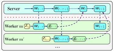
Figure 2: Schematic of the delayed gradient algorithms. While worker $m$ is computing and uploading the gradient, the server has performed $\tau$ asynchronous model updates.

To find a solution for the ERM problem (1), delayed gradient methods initialize the model parameters to $\mathbf{w}_{0}=\mathbf{w}_{1}=\cdots=\mathbf{w}_{\tau}$ and then iteratively update them with gradient descent. Figure 2 illustrates that the model $\mathbf{w}_{t}$ is updated with the stale gradient $\mathbf{g}_{t-\tau}$ at the $t$-th iteration, implying an iterative format of $\mathbf{w}_{t+1}=\mathbf{w}_{t}-\eta\mathbf{g}_{t-\tau}$ where $t>\tau$. In SGD, the delayed gradient $\mathbf{g}_{t-\tau}$ is evaluated on a randomly selected data point $\mathbf{z}_{i_{t}}$, and also constitutes a noisy gradient oracle of the empirical risk $F_{\mathcal{S}}$, i.e.,

$$\mathbf{g}_{t-\tau}=\nabla f(\mathbf{w}_{t-\tau};\mathbf{z}_{i_{t}})=\nabla F_{\mathcal{S}}(\mathbf{w}_{t-\tau})+\bm{\xi}_{t},$$ (2)

where $\bm{\xi}_{t}$ represents the associated stochastic noise. Delayed SGD updates the model parameters as

$$\begin{split}\mathbf{w}_{t+1}&=\mathbf{w}_{t}-\eta\nabla f(\mathbf{w}_{t-\tau};\mathbf{z}_{i_{t}})\\ &=\mathbf{w}_{t}-\eta\left(\nabla F_{\mathcal{S}}(\mathbf{w}_{t-\tau})+\bm{\xi}_{t}\right).\end{split}$$ (3)

3.3 Stability and generalization

Algorithm stability is a powerful tool for studying generalization. It estimates the generalization error of an algorithm by assessing the effect of changing a single sample in the training set on the output. Denote by $\mathcal{S}^{\prime}=\{\mathbf{z}_{1}^{\prime},\ldots,\mathbf{z}_{n}^{\prime}\}$ the set of random samples drawn i.i.d. from distribution $\mathcal{D}$ and independent of $\mathcal{S}$. Let $\mathcal{S}^{(i)}=\{\mathbf{z}_{1},\ldots,\mathbf{z}_{i-1},\mathbf{z}_{i}^{\prime},\mathbf{z}_{i+1},\ldots,\mathbf{z}_{n}\}$ be the replica of the sample $\mathcal{S}$ except in the $i$-th example, where we substitute $\mathbf{z}_{i}$ with $\mathbf{z}_{i}^{\prime}$. In this paper, we employ the following average stability framework Shalev-Shwartz et al. (2010).

Definition 1 (average stability).

A stochastic learning algorithm $\mathcal{A}$ is $\epsilon_{\text{stab}}$-average stable if for any datasets $\mathcal{S}$, $\mathcal{S}^{(i)}$ which differ in one example, we have

$$\left|\frac{1}{n}\sum_{i=1}^{n}\mathbb{E}_{\mathcal{S},\mathcal{S}^{\prime},\mathcal{A}}\left[f(\mathcal{A}(\mathcal{S});\mathbf{z}_{i}^{\prime})-f(\mathcal{A}(\mathcal{S}^{(i)});\mathbf{z}_{i}^{\prime})\right]\right|\leq\epsilon_{\text{stab}}.$$

The following lemma establishes the connection between average stability and generalization error (Shalev-Shwartz et al., 2010, Lemma 11).

Lemma 1.

Let algorithm $\mathcal{A}$ be $\epsilon_{\text{stab}}$-average stable. Then the generalization error satisfies

$$\left|\mathbb{E}_{\mathcal{S},\mathcal{A}}\left[F(\mathcal{A}(\mathcal{S}))-F_{\mathcal{S}}(\mathcal{A}(\mathcal{S}))\right]\right|\leq\epsilon_{\text{stab}}.$$

Remark 1.

Since for any $i$, $\mathbf{z}_{i}$ and $\mathbf{z}_{i}^{\prime}$ are both drawn i.i.d. from distribution $\mathcal{D}$, then $\mathcal{A}(\mathcal{S}^{(i)})$ is independent of $\mathbf{z}_{i}$, and the average stability can be formulated as

$$\left|\frac{1}{n}\sum_{i=1}^{n}\mathbb{E}_{\mathcal{S},\mathcal{S}^{\prime},\mathcal{A}}\left[f(\mathcal{A}(\mathcal{S}^{(i)});\mathbf{z}_{i})-f(\mathcal{A}(\mathcal{S});\mathbf{z}_{i})\right]\right|\leq\epsilon_{\text{stab}}.$$ (4)

This formulation is equivalent to Definition 1 and shares the property outlined in Lemma 1. We have provided a detailed analytical proof in the Appendix.

Therefore, our goal turns to study the average stability of the algorithm, which is sufficient to bound the generalization error. Before exploring the average stability and generalization error of the delayed stochastic gradient descent algorithm, we make the following regularity assumptions.

Assumption 1 (smoothness).

The loss function $F_{\mathcal{S}}$ is $\mu$-smooth, i.e., there exists a constant $\mu\in\mathbb{R}$ such that for any $\mathbf{w},\mathbf{v}\in\mathbb{R}^{d}$,

$$\|\nabla F_{\mathcal{S}}(\mathbf{w})-\nabla F_{\mathcal{S}}(\mathbf{v})\|\|\leq\mu\|\mathbf{w}-\mathbf{v}\|.$$

Assumption 2 (bounded space).

The mean of the sample points in the training data set is bounded, i.e., $\mathbb{E}_{\mathcal{S}}[\|\mathbf{b}\|]\leq r$, where $r\in\mathbb{R}$ is a constant, and $\mathbf{b}=\frac{1}{n}\sum_{i=1}^{n}-y_{i}\mathbf{x}_{i}\in\mathbb{R}^{d}$.

Assumption 3 (bounded noise).

For stochastic algorithm $\mathcal{A}$, the stochastic noise $\bm{\xi}_{t}$ is bounded, i.e., there exists a constant $\sigma\in\mathbb{R}$ such that $\mathbb{E}_{\mathcal{S},\mathcal{A}}[\|\bm{\xi}_{t}\|]\leq\sigma$.

Assumption 1 is to bound the eigenvalues of the matrix $\mathbf{A}$, i.e., $\max_{j\in[d]}a_{j}<\mu$, which is natural in quadratic problems. Assumption 2 typically holds in supervised machine learning applications. In stochastic algorithms, it is common to assume that the random noise is bounded, independent, and has zero mean. However, in this paper, we only require the noise to be bounded (Assumption 3).

4 Average stability via generating function derivations

This section focuses on analyzing the average stability of the delayed stochastic gradient descent algorithm with fixed delay $\tau$, and the derivation is generalized to random delays in Section 6. To measure the algorithmic stability, we run the delayed SGD algorithm on two datasets $\mathcal{S}$ and $\mathcal{S}^{(i)}$ from the same starting point, and obtain the models $\mathbf{w}_{t}$ and $\mathbf{w}_{t}^{\prime}$ after $t$ iterations, respectively. According to Definition (4), the average stability under the quadratic loss function can be formulated as

$$\begin{split}&\mathbb{E}\left|\frac{1}{n}\sum_{i=1}^{n}\left[f(\mathbf{w}_{t}^{\prime};\mathbf{z}_{i})-f(\mathbf{w}_{t};\mathbf{z}_{i})\right]\right|=\mathbb{E}\left|\frac{1}{2}(\mathbf{w}_{t}^{\prime}-\mathbf{w}_{t})^{\top}\mathbf{A}(\mathbf{w}_{t}^{\prime}+\mathbf{w}_{t})+\mathbf{b}^{\top}(\mathbf{w}_{t}^{\prime}-\mathbf{w}_{t})\right|\\ &\leq\frac{1}{2}\mathbb{E}\left|(\mathbf{w}_{t}^{\prime}-\mathbf{w}_{t})^{\top}\mathbf{A}(\mathbf{w}_{t}^{\prime}+\mathbf{w}_{t})\right|+\mathbb{E}\|\mathbf{b}\|\|\mathbf{w}_{t}^{\prime}-\mathbf{w}_{t}\|\\ &\leq\frac{1}{2}\mathbb{E}\left\|\sqrt{\mathbf{A}}\mathbf{e}_{t}\right\|\left\|\sqrt{\mathbf{A}}\mathbf{s}_{t}\right\|+\mathbb{E}\|\mathbf{b}\|\|\mathbf{e}_{t}\|.\end{split}$$ (5)

Here we defined two crucial symbols $\mathbf{e}_{t}=\mathbf{w}_{t}-\mathbf{w}_{t}^{\prime}$ and $\mathbf{s}_{t}=\mathbf{w}_{t}+\mathbf{w}_{t}^{\prime}$. It is worth noting that this section investigates the algorithmic stability, hence all the notations $\mathbb{E}$ in this section take expectations with respect to the randomness of $\mathcal{S},\mathcal{S}^{\prime}$ and $\mathcal{A}$, consistent with Definition 1. Since the two iterations start from the same model, i.e., $\mathbf{w}_{0}=\mathbf{w}_{0}^{\prime}$, and combined with the initial setup $\mathbf{w}_{0}=\cdots=\mathbf{w}_{\tau}$ yields

$$\begin{split}\mathbf{e}_{0}=\mathbf{e}_{1}=\cdots=\mathbf{e}_{\tau}=\mathbf{0}~{}~{}\text{and}~{}~{}\mathbf{s}_{0}=\mathbf{s}_{1}=\cdots=\mathbf{s}_{\tau}.\end{split}$$ (6)

Recalling that $\mathbf{w}_{t+1}$ is obtained from $\mathbf{w}_{t}$ via delayed gradient updates (3), our goal is to establish recursive properties of the sequences $\{\mathbf{e}_{t}\}_{t}$ and $\{\mathbf{s}_{t}\}_{t}$ based on the iterative behavior of the algorithm. Two cases arise at each iteration for the sequence $\{\mathbf{e}_{t}\}_{t}$. In the first case, the sample selected on the datasets $\mathcal{S}$ and $\mathcal{S}^{(i)}$ is identical, meaning that the data index $i_{t}\neq i$. Since the datasets containing $n$ samples have only one data that is different, the probability of this situation occurring is $1-1/n$. We directly calculate the gradients of the quadratic loss function, which evaluate models $\mathbf{w}$ and $\mathbf{w}^{\prime}$ on the same data $\mathbf{z}_{i_{t}}$, and the following equation can be obtained.

$$\begin{split}&\mathbb{E}[\mathbf{e}_{t+1}]=\mathbb{E}[\mathbf{w}_{t+1}-\mathbf{w}_{t+1}^{\prime}]=\mathbb{E}[\mathbf{w}_{t}-\mathbf{w}_{t}^{\prime}]-\eta\mathbb{E}\left[\nabla f(\mathbf{w}_{t-\tau};\mathbf{z}_{i_{t}})-\nabla f(\mathbf{w}_{t-\tau}^{\prime};\mathbf{z}_{i_{t}})\right]\\ &=\mathbb{E}[\mathbf{e}_{t}]-\eta\mathbb{E}\left[\mathbf{x}_{i_{t}}\mathbf{x}_{i_{t}}^{\top}(\mathbf{w}_{t-\tau}-\mathbf{w}_{t-\tau}^{\prime})\right]=\mathbb{E}[\mathbf{e}_{t}]-\eta\mathbb{E}[\mathbf{A}\mathbf{e}_{t-\tau}],\end{split}$$

where the last equality is due to the fact that $\mathbf{z}_{i_{t}}$ is independent of $\mathbf{w}_{t-\tau}-\mathbf{w}_{t-\tau}^{\prime}$ and the expectation on the training data set $\mathcal{S}$. The second case is that the algorithm exactly selects the $i$-th sample point which is different in the two datasets. Note that this happens only with probability $1/n$ in the random selection setup. In this case, we use the gradient containing noise to quantify the effect of different samples $\mathbf{z}_{i}$ and $\mathbf{z}_{i}^{\prime}$ on the sequence.

$$\begin{split}&\mathbb{E}[\mathbf{e}_{t+1}]=\mathbb{E}[\mathbf{w}_{t+1}-\mathbf{w}_{t+1}^{\prime}]=\mathbb{E}[\mathbf{w}_{t}-\mathbf{w}_{t}^{\prime}]-\eta\mathbb{E}\left[\mathbf{A}\mathbf{w}_{t-\tau}+\mathbf{b}+\bm{\xi}_{t}-(\mathbf{A}\mathbf{w}_{t-\tau}^{\prime}+\mathbf{b}+\bm{\xi}_{t}^{\prime})\right]\\ &=\mathbb{E}[\mathbf{e}_{t}]-\eta\mathbb{E}[\mathbf{A}\mathbf{e}_{t-\tau}]-\eta\mathbb{E}[\bm{\xi}_{t}-\bm{\xi}_{t}^{\prime}].\end{split}$$

Here, $\bm{\xi}_{t}^{\prime}$ is the gradient noise with respect to $F_{\mathcal{S}}(\mathbf{w}_{t-\tau}^{\prime})$ instead of $F_{\mathcal{S}^{(i)}}(\mathbf{w}_{t-\tau}^{\prime})$. Since $\mathcal{S}$ and $\mathcal{S}^{(i)}$ differ by only one data point, the expect difference between $F_{\mathcal{S}}(\mathbf{w}_{t-\tau}^{\prime})$ and $F_{\mathcal{S}^{(i)}}(\mathbf{w}_{t-\tau}^{\prime})$ is of order $\mathcal{O}(1/n)$, hence $\bm{\xi}_{t}^{\prime}$ also satisfies the bounded noise assumption. Combining the two cases and taking expectation for $\mathbf{e}_{t+1}$ with respect to the randomness of the algorithm, we derive the recurrence relation

$$\mathbb{E}[\mathbf{e}_{t+1}]=\mathbb{E}[\mathbf{e}_{t}]-\eta\mathbb{E}[\mathbf{A}\mathbf{e}_{t-\tau}]-\frac{\eta}{n}\mathbb{E}[\bm{\xi}_{t}-\bm{\xi}_{t}^{\prime}].$$ (7)

For the sequence $\{\mathbf{s}_{t}\}_{t}$, we do not need to examine them separately. The iterative format (3) of delayed SGD produces the following equation.

$$\begin{split}&\mathbb{E}[\mathbf{s}_{t+1}]=\mathbb{E}[\mathbf{w}_{t+1}+\mathbf{w}_{t+1}^{\prime}]=\mathbb{E}[\mathbf{w}_{t}+\mathbf{w}_{t}^{\prime}]-\eta\mathbb{E}\left[\mathbf{A}\mathbf{w}_{t-\tau}+\mathbf{b}+\bm{\xi}_{t}+(\mathbf{A}\mathbf{w}_{t-\tau}^{\prime}+\mathbf{b}+\bm{\xi}_{t}^{\prime})\right]\\ &=\mathbb{E}[\mathbf{s}_{t}]-\eta\mathbb{E}[\mathbf{A}\mathbf{s}_{t-\tau}]-\eta\mathbb{E}[2\mathbf{b}+\bm{\xi}_{t}+\bm{\xi}_{t}^{\prime}].\end{split}$$ (8)

The well-established equational recurrence formulas for sequences $\{\mathbf{e}_{t}\}_{t}$ and $\{\mathbf{s}_{t}\}_{t}$ motivate us to study them using the generating function tool. Generally speaking, the generating function of a given sequence $\{\bm{\alpha}_{t}\}_{t}$ is a formal power series $\bm{\varphi}(x)=\sum_{t=0}^{\infty}\bm{\alpha}_{t}x^{t}$. Note that the variable $x$ in generating functions serves as a placeholder to track coefficients without standing for any particular value. We define $[x^{t}]\bm{\varphi}(x)$ as the operation that extracts the coefficient of $x^{t}$ in the formal power series $\bm{\varphi}(x)$, i.e., $\bm{\alpha}_{t}=[x^{t}]\bm{\varphi}(x)$. Generating functions are frequently the most efficient and concise way to present information about their coefficients, and have been used to study optimization errors of delayed gradient methods Arjevani et al. (2020). Details on generating functions can be found in Wilf (1990); Stanley and Fomin (1999); Flajolet and Sedgewick (2009).

Remark 2.

Arjevani et al. Arjevani et al. (2020) investigated the optimization error, i.e., $F_{\mathcal{S}}(\mathbf{w}_{T})-F_{\mathcal{S}}(\mathbf{w}^{*})$, of the delayed SGD algorithm, where $\mathbf{w}^{*}$ is the minimizer of $F_{\mathcal{S}}$. They used the crucial property $\nabla F_{\mathcal{S}}(\mathbf{w}^{*})=\bm{0}$ to construct the equational recursive sequence so that it can be analyzed with the generating functions. This paper, however, studies the generalization error, i.e., $F(\mathbf{w}_{T})-F_{\mathcal{S}}(\mathbf{w}_{T})$, which is not relevant to $\mathbf{w}^{*}$, and thus is quite different from Arjevani et al. (2020) in constructing the equational recursive relations. We ingeniously formulate different formats of the delayed stochastic gradient, denoted as (2), and employ them flexibly to derive the average stability, yielding equational recurrence formulas (7) and (8) for sequences $\{\mathbf{e}_{t}\}_{t}$ and $\{\mathbf{s}_{t}\}_{t}$, respectively.

Let $\bm{\phi}(x)$ and $\bm{\psi}(x)$ be the generating functions of sequences $\{\mathbf{e}_{t}\}_{t}$ and $\{\mathbf{s}_{t}\}_{t}$, respectively, defined as

$$\bm{\phi}(x)=\sum_{t=0}^{\infty}\mathbf{e}_{t}x^{t}~{}~{}\text{and}~{}~{}\bm{\psi}(x)=\sum_{t=0}^{\infty}\mathbf{s}_{t}x^{t}.$$

The expectation notation is omitted in the derivation of the generating function for the sake of brevity. According to recurrence formula (7), the generating function $\bm{\phi}(x)$ proceeds as

$$\begin{split}&\bm{\phi}(x)=\sum_{t=0}^{\tau}\mathbf{e}_{t}x^{t}+\sum_{t=\tau+1}^{\infty}\mathbf{e}_{t}x^{t}\overset{(\star)}{=}\sum_{t=\tau+1}^{\infty}\left[\mathbf{e}_{t-1}-\eta\mathbf{A}\mathbf{e}_{t-\tau-1}-\frac{\eta}{n}(\bm{\xi}_{t-1}-\bm{\xi}_{t-1}^{\prime})\right]x^{t}\\ &\overset{(\star)}{=}x\bm{\phi}(x)-\eta\mathbf{A}x^{\tau+1}\bm{\phi}(x)-\frac{\eta}{n}\sum_{t=\tau}^{\infty}(\bm{\xi}_{t}-\bm{\xi}_{t}^{\prime})x^{t+1},\end{split}$$ (9)

where $(\star)$ uses the initialization (6). Similarly, the generating function $\bm{\psi}(x)$ can deduce the following property based on equation (8).

$$\begin{split}&\bm{\psi}(x)=\sum_{t=0}^{\tau}\mathbf{s}_{t}x^{t}+\sum_{t=\tau+1}^{\infty}\Big{[}\mathbf{s}_{t-1}-\eta\mathbf{A}\mathbf{s}_{t-\tau-1}-\eta(2\mathbf{b}+\bm{\xi}_{t-1}+\bm{\xi}_{t-1}^{\prime})\Big{]}x^{t}\\ &\overset{(\star)}{=}\mathbf{s}_{0}+x\bm{\psi}(x)-\eta\mathbf{A}x^{\tau+1}\bm{\psi}(x)-\eta\sum_{t=\tau}^{\infty}(2\mathbf{b}+\bm{\xi}_{t}+\bm{\xi}_{t}^{\prime})x^{t+1}.\end{split}$$ (10)

Abbreviating the last terms in equations (9) and (10) as the power series $\mathbf{u}(x)$ and $\mathbf{v}(x)$, i.e.,

$$\mathbf{u}(x)=\sum_{t=\tau}^{\infty}(\bm{\xi}_{t}^{\prime}-\bm{\xi}_{t})x^{t+1}~{}~{}\text{and}~{}~{}\mathbf{v}(x)=\sum_{t=\tau}^{\infty}(2\mathbf{b}+\bm{\xi}_{t}+\bm{\xi}_{t}^{\prime})x^{t+1}.$$

Rearranging the terms in equations (9) and (10), we arrive at

$$(\mathbf{I}-\mathbf{I}x+\eta\mathbf{A}x^{\tau+1})\bm{\phi}(x)=\frac{\eta}{n}\mathbf{u}(x)~{}~{}\text{and}~{}~{}(\mathbf{I}-\mathbf{I}x+\eta\mathbf{A}x^{\tau+1})\bm{\psi}(x)=\mathbf{s}_{0}-\eta\mathbf{v}(x),$$

where $\mathbf{I}\in\mathbb{R}^{d\times d}$ is the identity matrix. Below we introduce some algebraic notations for studying generating functions. $\mathbb{R}[[x]]$ represents the set of all formal power series in the indeterminate $x$ with coefficients belonging to the reals $\mathbb{R}$. It is equipped with standard addition and multiplication (Cauchy product) operations, forming a commutative ring. The set of all matrices in $\mathbb{R}^{d\times d}$ is denoted as $\mathcal{M}_{d}(\mathbb{R})$, and $\mathcal{M}_{d}(\mathbb{R})[[x]]$ is the set of matrices with elements in $\mathbb{R}[[x]]$, which also forms a ring of formal power series with real matrix coefficients. According to (Wilf, 1990, Proposition 2.1), $\mathbf{I}-\mathbf{I}x+\eta\mathbf{A}x^{\tau+1}$ is invertible in $\mathcal{M}_{d}(\mathbb{R})[[x]]$, as the constant term $\mathbf{I}$ is invertible in $\mathcal{M}_{d}(\mathbb{R})$. Denote the inverse of $\mathbf{I}-\mathbf{I}x+\eta\mathbf{A}x^{\tau+1}$ as the power series $\bm{\pi}(x)$, namely

$$\bm{\pi}(x)=(\mathbf{I}-\mathbf{I}x+\eta\mathbf{A}x^{\tau+1})^{-1},$$ (11)

then the following concise properties are observed for the generating functions $\bm{\phi}(x)$ and $\bm{\psi}(x)$.

$$\bm{\phi}(x)=\frac{\eta}{n}\bm{\pi}(x)\cdot\mathbf{u}(x)~{}~{}\text{and}~{}~{}\bm{\psi}(x)=\bm{\pi}(x)\cdot\left[\mathbf{s}_{0}-\eta\mathbf{v}(x)\right].$$

Returning to the average stability (5) of the delayed SGD algorithm, we can extract the corresponding coefficients in generating functions, i.e., $\mathbf{e}_{t}=[x^{t}]\bm{\phi}(x),\mathbf{s}_{t}=[x^{t}]\bm{\psi}(x)$, to analyze the terms in (5).

$$\begin{split}&\mathbb{E}\|\mathbf{e}_{t}\|=\frac{\eta}{n}\mathbb{E}\left\|[x^{t}](\bm{\pi}(x)\cdot\mathbf{u}(x))\right\|\overset{(i)}{=}\frac{\eta}{n}\mathbb{E}\left\|\sum_{i=0}^{t-\tau-1}\left([x^{i}]\bm{\pi}(x)\right)(\bm{\xi}_{t-i-1}^{\prime}-\bm{\xi}_{t-i-1})\right\|\\ &\overset{(ii)}{\leq}\frac{2\eta\sigma}{n}\mathbb{E}\left\|\sum_{i=0}^{t-\tau-1}[x^{i}]\bm{\pi}(x)\right\|\leq\frac{2\eta\sigma}{n}\sum_{i=0}^{t-\tau-1}\mathbb{E}\left\|[x^{i}]\bm{\pi}(x)\right\|,\end{split}$$

where $(i)$ utilizes the Cauchy product for formal power series, and $(ii)$ is based on Assumptions 3. Analogously, we have

$$\mathbb{E}\|\sqrt{\mathbf{A}}\mathbf{e}_{t}\|\leq\frac{2\eta\sigma}{n}\sum_{i=0}^{t-\tau-1}\mathbb{E}\|\sqrt{\mathbf{A}}[x^{i}]\bm{\pi}(x)\|.$$

$$\begin{split}&\mathbb{E}\|\sqrt{\mathbf{A}}\mathbf{s}_{t}\|=\mathbb{E}\left\|\sqrt{\mathbf{A}}[x^{t}](\bm{\pi}(x)(\mathbf{s}_{0}-\eta\mathbf{v}(x)))\right\|\overset{(i)}{\leq}\mathbb{E}\left\|\sqrt{\mathbf{A}}[x^{t}]\bm{\pi}(x)\mathbf{s}_{0}\right\|+\eta\mathbb{E}\left\|\sqrt{\mathbf{A}}[x^{t}](\bm{\pi}(x)\mathbf{v}(x))\right\|\\ &\overset{(ii)}{\leq}\mathbb{E}\left\|\sqrt{\mathbf{A}}[x^{t}]\bm{\pi}(x)\mathbf{s}_{0}\right\|+2\eta(r+\sigma)\sum_{i=0}^{t-\tau-1}\mathbb{E}\left\|\sqrt{\mathbf{A}}[x^{i}]\bm{\pi}(x)\right\|,\end{split}$$

where $(i)$ uses the linearity of the extraction operation $[x^{t}]$, and $(ii)$ follows by the Cauchy product and Assumptions 2, 3. Finally, we derive the following average stability bound of delayed SGD.

Proposition 1.

Let Assumptions 2, 3 hold and the loss function $F_{\mathcal{S}}$ be quadratic, i.e., $F_{\mathcal{S}}(\mathbf{w})=\frac{1}{2}\mathbf{w}^{\top}\mathbf{A}\mathbf{w}+\mathbf{b}^{\top}\mathbf{w}+c$, then the average stability $\epsilon_{\text{stab}}$ of delayed SGD after $t$ iterations ($t>\tau$) satisfies

$$\begin{split}\epsilon_{\text{stab}}\leq&\frac{2\eta r\sigma}{n}\sum_{i=0}^{t-\tau-1}\mathbb{E}\left\|[x^{i}]\bm{\pi}(x)\right\|+\frac{2\eta\sigma\left\|\mathbf{w}_{0}\right\|}{n}\mathbb{E}\left\|\sqrt{\mathbf{A}}[x^{t}]\bm{\pi}(x)\right\|\sum_{i=0}^{t-\tau-1}\mathbb{E}\left\|\sqrt{\mathbf{A}}[x^{i}]\bm{\pi}(x)\right\|\\ &+\frac{2\eta^{2}\sigma(r+\sigma)}{n}\left(\sum_{i=0}^{t-\tau-1}\mathbb{E}\left\|\sqrt{\mathbf{A}}[x^{i}]\bm{\pi}(x)\right\|\right)^{2}.\end{split}$$ (12)

5 Generalization error of delayed stochastic gradient descent

According to Lemma 1 and the average stability (12), the generalization error is followed by estimating the coefficients of the power series $\bm{\pi}(x)$, which is defined in (11). Inspired by (Arjevani et al., 2020, Lemma 1), we can obtain the subsequent lemma to bound $\|[x^{t}]\bm{\pi}(x)\|$. Then we are ready to present the generalization error of delayed SGD, including the convex and strongly convex quadratic objectives. All the proof details are included in the Appendixs.

Lemma 2.

Let Assumption 1 holds and the learning rate $\eta\in(0,1/\mu\tau]$. Then the $t$-th coefficient of the power series $\bm{\pi}(x)$ satisfies $\|[x^{t}]\bm{\pi}(x)\|\leq 1$ for any $t\geq 0$. Furthermore, if $\eta\in(0,1/20\mu(\tau+1)]$, we have

$$\left\{\begin{array}[]{ll}\vspace{1.3ex}\left\|[x^{t}]\bm{\pi}(x)\right\|\leq 1&~{}~{}0\leq t\leq t_{0}-1,\\ \left\|[x^{t}]\bm{\pi}(x)\right\|\leq 3\max_{j\in[d]}(1-\eta a_{j})^{t+1}&~{}~{}t\geq t_{0}.\end{array}\right.$$

where $t_{0}=(\tau+1)\ln(2(\tau+1))$ and $a_{j}$ is the $j$-th eigenvalue of the positive semi-definite matrix $\mathbf{A}$.

Theorem 1.

Let Assumptions 1-3 hold, and the learning rate $\eta\in(0,1/20\mu(\tau+1)]$, then the generalization error (or average stability) of delayed SGD after $T$ iterations satisfies

$$\begin{split}\mathbb{E}_{\mathcal{S},\mathcal{A}}[F(\mathbf{w}_{T})-F_{\mathcal{S}}(\mathbf{w}_{T})]&\leq\frac{\sigma(r+\sigma)}{n\mu}\left[\sqrt{T-\tau}+12\mu\left\|\mathbf{w}_{0}\right\|+\ln^{2}(\tau+1)\right]+\frac{\sigma(r+\sigma)}{n\mu\tau}(T-\tau)\\ &\leq\tilde{\mathcal{O}}\left(\frac{T-\tau}{n\tau}\right).\end{split}$$

For the quadratic problem, Theorem 1 indicates that the algorithmic stability of delayed SGD is positively correlated with the delay $\tau$ provided the learning rate satisfies $\eta\leq 1/20\mu(\tau+1)$, meaning that asynchronous delay makes SGD more stable and hence reduces the generalization error. It follows that asynchronous delay enables the model to perform more consistently across the training and test datasets. The next theorem demonstrates that the generalization error is independent of the iteration number $T$ if the quadratic function is further strongly convex.

Theorem 2.

Suppose the quadratic function is $\lambda$-strongly convex, and Assumptions 1-3 hold. Let the learning rate $\eta\in(0,1/20\mu(\tau+1)]$, then the generalization error of delayed SGD is bounded by

$$\begin{split}\frac{2\sigma(r+\sigma)\eta t_{0}}{n}\left[1+3\mu\left\|\mathbf{w}_{0}\right\|+\mu\eta t_{0}+12\sqrt{\frac{\mu}{e\lambda}}\right]+\frac{42\sigma(r+\sigma)}{n\lambda}+\frac{36\sigma\left\|\mathbf{w}_{0}\right\|}{n}\sqrt{\frac{\mu}{e\lambda}}=\tilde{\mathcal{O}}\left(\frac{1}{n}\right).\end{split}$$

Additionally, both Theorems 1 and 2 suggest that increasing the training samples amount $n$ can stabilize the algorithm and thus decrease the generalization error.

Remark 3.

Under the bounded gradient assumption, Hardt et al. (2016) provides upper bounds on the generalization error of plain SGD for both general convex and strongly convex cases as $\mathcal{O}(\frac{T}{n})$ and $\mathcal{O}(\frac{1}{n})$, respectively, and these upper bounds are subsequently shown to be tight Zhang et al. (2022). This is consistent with our results in the synchronous case (i.e., $\tau=1$).

Remark 4.

It is worth mentioning that the proven results also benefit the understanding of delayed or synchronous algorithms for deep neural network (DNN) training though they are established for quadratic functions. The reason lies in the neural tangent kernel (NTK) approach Jacot et al. (2018); Lee et al. (2019), which promises that the dynamics of gradient descent on DNNs are close to those on quadratic optimization under sufficient overparameterization and random initialization.

Remark 5.

Denote $\mathbf{w}_{*}$ as the minimizer of population risk $F$, and $F(\mathbf{w}_{T})-F(\mathbf{w}_{*})$ is known as the excess generalization error, which is bounded by the sum of the generalization error and the optimization error Hardt et al. (2016). Together with the optimization results of Arjevani et al. (2020), we can derive upper bounds for the excess generalization error of delayed SGD, namely, $\tilde{\mathcal{O}}(\frac{1}{\sqrt{T}}+\frac{T-\tau}{n\tau})$ for convex and $\tilde{\mathcal{O}}(\frac{1}{T}+\frac{1}{n})$ for strongly convex quadratic loss function. The results suggest that when solving convex quadratic problems, training should be stopped at the proper time, i.e., choosing an appropriate $T$ to balance the optimization and generalization errors so that the excess generalization error is minimized. While in the strongly convex case, sufficient training can be performed to reduce optimization errors and improve the generalization performance.

6 Extension to random delays

This section shows how to extend the fixed delay $\tau$ to a dynamic scenario with the random delay $\tau_{t}$ for stochastic gradient descent. Specifically, the algorithm with random delay is formulated as

$$\mathbf{w}_{t+1}=\mathbf{w}_{t}-\eta\nabla f(\mathbf{w}_{t-\tau_{t}};\mathbf{z}_{i_{t}})=\mathbf{w}_{t}-\eta\left(\nabla F_{\mathcal{S}}(\mathbf{w}_{t-\tau_{t}})+\bm{\xi}_{t}\right),$$

where $\tau_{t}$ is the random delay at $t$-th iteration, and the standard bounded delay assumption is required.

Assumption 4 (bounded delay).

The random delay is bounded, i.e., there exists a constant $\overline{\tau}\in\mathbb{R}$ such that $\tau_{t}\leq\overline{\tau}$ for all iteration $t$.

To start the training process, we initialize the delayed algorithm as $\mathbf{w}_{0}=\cdots=\mathbf{w}_{\overline{\tau}}$. Then we follow the same notation $\mathbf{e}_{t}=\mathbf{w}_{t}-\mathbf{w}_{t}^{\prime}$ and $\mathbf{s}_{t}=\mathbf{w}_{t}+\mathbf{w}_{t}^{\prime}$ in Section 4. The equational recurrence formulas on sequences $\{\mathbf{e}_{t}\}_{t}$ and $\{\mathbf{s}_{t}\}_{t}$ are identical to (7) and (8), except that the fixed delay $\tau$ is replaced by the random delay $\tau_{t}$. The related generating functions, $\bm{\phi}(x)$ and $\bm{\psi}(x)$, are determined as

$$\begin{split}\bm{\phi}(x)&=x\bm{\phi}(x)-\eta\mathbf{A}x^{\overline{\tau}+1}\bm{\phi}(x)-\eta\sum_{t=\overline{\tau}}^{\infty}\Big{[}\frac{1}{n}(\bm{\xi}_{t}-\bm{\xi}_{t}^{\prime})+\bm{\zeta}_{t}-\bm{\zeta}_{t}^{\prime}\Big{]}x^{t+1},\\ \bm{\psi}(x)&=\mathbf{s}_{0}+x\bm{\psi}(x)-\eta\mathbf{A}x^{\overline{\tau}+1}\bm{\psi}(x)-\eta\sum_{t=\overline{\tau}}^{\infty}(2\mathbf{b}+\bm{\xi}_{t}+\bm{\xi}_{t}^{\prime}+\bm{\zeta}_{t}+\bm{\zeta}_{t}^{\prime})x^{t+1},\end{split}$$

where $\bm{\zeta}_{t}$ and $\bm{\zeta}_{t}^{\prime}$ measure the magnitude of model differences $\mathbf{w}_{t-\tau_{t}}-\mathbf{w}_{t-\overline{\tau}}$ and $\mathbf{w}_{t-\tau_{t}}^{\prime}-\mathbf{w}_{t-\overline{\tau}}^{\prime}$, respectively. Due to the convergence property of delayed SGD (Mishchenko et al., 2022) and the bounded delay Assumption 4, it is reasonable to conclude that $\bm{\zeta}_{t}$ and $\bm{\zeta}_{t}^{\prime}$ are bounded. By extracting the corresponding coefficients of the generating functions to analyze average stability (5), we can establish the generalization error bounds of the delayed SGD algorithm with random delay.

Corollary 1.

Let Assumptions 1-4 hold, and the learning rate $\eta\in(0,1/20\mu(\overline{\tau}+1)]$, then we can derive the generalization error bounds of delayed SGD with random delays for the convex case $\tilde{\mathcal{O}}(\frac{T-\overline{\tau}}{n\overline{\tau}})$ and the strongly convex case $\tilde{\mathcal{O}}(\frac{1}{n})$, respectively.

7 Experimental validation

In this section, we conduct simulation experiments to validate our theoretical findings for the quadratic convex model (1), where the generalization error plotted is the difference between the training loss and the testing loss. We used four classical datasets from the LIBSVM database (Chang and Lin, 2011), namely rcv1 ($d=47,236$, $n=20,242$), gisette ($d=5,000$, $n=6,000$), covtype ($d=54$, $n=581,012$) and ijcnn1 ($d=22$, $n=49,990$). In our simulations, we employed 16 distributed workers with a single local batch size of 16. Note that we fixed all parameters except the asynchronous delay in each experiment and utilized a constant learning rate. Furthermore, all experiments were reproduced five times with different random seeds.

Figures 3(a) and 3(b) present the results for random delays, with the legend representing the maximum delay $\overline{\tau}$, while Figures 3(c) and 3(d) illustrate the generalization errors with fixed $4,8,16,32$ delays. As shown in the figures, the generalization error grows with the iterations of the algorithm, but increasing the asynchronous delay makes this error decrease, which is consistent with our theoretical findings. Additionally, we showcase the training and testing loss curves in Figures 3(e) and 3(f), indicating that the asynchronous delay mitigates the overfitting phenomenon when the model converges, thereby leading to a decreased generalization error.

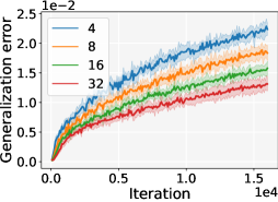
(a) Gen. error of rcv1

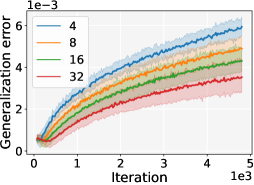
(b) Gen. error of gisette

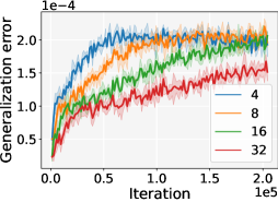
(c) Gen. error of covtype

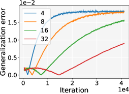
(d) Gen. error of ijcnn1

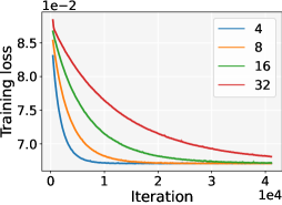
(e) Training loss of ijcnn1

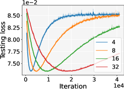
(f) Testing loss of ijcnn1

Figure 3: Experimental results for solving quadratic convex problems with delayed SGD. We test the generalization error of different delays on four LIBSVM datasets rcv1, gisette, covtype and ijcnn1, and set the learning rates to constant values of $0.05$, $0.00001$, $0.0005$ and $0.01$, respectively. The variance in the plots is due to selecting different random seeds in multiple trials.

8 Conclusion and future work

In this paper, we study the generalization performance of the delayed stochastic gradient descent algorithm. For the quadratic problem, we use the generating functions to derive the average stability of SGD with fixed and random delays. Building on the algorithmic stability, we provide sharper generalization error bounds for delayed SGD in the convex and strongly convex cases. Our theoretical results indicate that asynchronous delays make SGD more stable and hence reduce the generalization error. The corresponding experiments corroborate our theoretical findings.

In practice, the delayed gradient method exhibits similar generalization performance in non-convex problems, as illustrated in Figure 1. Therefore, our current findings may be extended to the widespread non-convex applications in the future. Additionally, SGD is proven to be robust to arbitrary delays in the optimization theory (Cohen et al., 2021; Mishchenko et al., 2022). Hence an interesting direction for future research is to investigate the generalization performance of SGD with arbitrary delays.

Appendix for
Towards Understanding the Generalizability of Delayed Stochastic Gradient Descent

The Appendix provides detailed proofs of all theoretical results and complete experimental results.

Appendix A Theoretical proof details

A.1 Proof of Lemma 1

The proof is based on an argument in Lemma 11 of Shalev-Shwartz et al. (2010). For any $i$, the data samples $\mathbf{z}_{i}$ and $\mathbf{z}_{i}^{\prime}$ are both drawn i.i.d. from $\mathcal{D}$. We denote the sets

$$\mathcal{S}=\{\mathbf{z}_{1},\ldots,\mathbf{z}_{n}\},~{}\mathcal{S}^{\prime}=\{\mathbf{z}_{1}^{\prime},\ldots,\mathbf{z}_{n}^{\prime}\},~{}\text{and}~{}~{}\mathcal{S}^{(i)}=\{\mathbf{z}_{1},\ldots,\mathbf{z}_{i-1},\mathbf{z}_{i}^{\prime},\mathbf{z}_{i+1},\ldots,\mathbf{z}_{n}\}.$$

Due to the fact that

$$\begin{split}F(\mathcal{A}(\mathcal{S}))&=\mathbb{E}_{\mathcal{S}^{\prime}}[f(\mathcal{A}(\mathcal{S});\mathbf{z}_{i}^{\prime})]=\frac{1}{n}\sum_{i=1}^{n}\mathbb{E}_{\mathcal{S}^{\prime}}[f(\mathcal{A}(\mathcal{S});\mathbf{z}_{i}^{\prime})],\\ \mathbb{E}_{\mathcal{S}}[f(\mathcal{A}(\mathcal{S});\mathbf{z}_{i})]&=\mathbb{E}_{\mathcal{S},\mathcal{S}^{\prime}}[f(\mathcal{A}(\mathcal{S}^{(i)});\mathbf{z}_{i}^{\prime})].\end{split}$$ (13)

Hence,

$$\begin{split}\epsilon_{\text{gen}}=\mathbb{E}_{\mathcal{S},\mathcal{A}}\left[F(\mathcal{A}(\mathcal{S}))-F_{\mathcal{S}}(\mathcal{A}(\mathcal{S}))\right]&=\mathbb{E}_{\mathcal{S},\mathcal{A}}\left[\mathbb{E}_{\mathcal{S}^{\prime}}[f(\mathcal{A}(\mathcal{S});\mathbf{z}_{i}^{\prime})]-\frac{1}{n}\sum_{i=1}^{n}f(\mathcal{A}(\mathcal{S});\mathbf{z}_{i})\right]\\ &=\frac{1}{n}\sum_{i=1}^{n}\mathbb{E}_{\mathcal{S},\mathcal{A}}\Big{[}\mathbb{E}_{\mathcal{S}^{\prime}}[f(\mathcal{A}(\mathcal{S});\mathbf{z}_{i}^{\prime})]-f(\mathcal{A}(\mathcal{S});\mathbf{z}_{i})\Big{]}\\ &=\frac{1}{n}\sum_{i=1}^{n}\mathbb{E}_{\mathcal{S},\mathcal{S}^{\prime},\mathcal{A}}\left[f(\mathcal{A}(\mathcal{S});\mathbf{z}_{i}^{\prime})-f(\mathcal{A}(\mathcal{S}^{(i)});\mathbf{z}_{i}^{\prime})\right]\\ &\leq\epsilon_{\text{stab}}.\end{split}$$

$\hfill\blacksquare$

A.2 Proof of Remark 1

Since for any $i$, $\mathbf{z}_{i}$ and $\mathbf{z}_{i}^{\prime}$ are both drawn i.i.d. from $\mathcal{D}$, we can see that $\mathcal{A}(\mathcal{S}^{(i)})$ is independent of $\mathbf{z}_{i}$. Hence we can obtain the following fact, which is also applied in the proof of Lei and Ying (2020) (Appendix B of Lei and Ying (2020))

$$\mathbb{E}_{\mathcal{S}}[F(\mathcal{A}(\mathcal{S}))]=\mathbb{E}_{\mathcal{S},\mathcal{S}^{\prime}}[f(\mathcal{A}(\mathcal{S}^{(i)});\mathbf{z}_{i})]=\frac{1}{n}\sum_{i=1}^{n}\mathbb{E}_{\mathcal{S},\mathcal{S}^{\prime}}[f(\mathcal{A}(\mathcal{S}^{(i)});\mathbf{z}_{i})].$$ (14)

By leveraging facts (13) and (14), we can equivalently reformulate the definition of average stability (Definition 1) as

$$\left|\frac{1}{n}\sum_{i=1}^{n}\mathbb{E}_{\mathcal{S},\mathcal{S}^{\prime},\mathcal{A}}\left[f(\mathcal{A}(\mathcal{S}^{(i)});\mathbf{z}_{i})-f(\mathcal{A}(\mathcal{S});\mathbf{z}_{i})\right]\right|\leq\epsilon_{\text{stab}}.$$ (15)

Furthermore, based on established facts (13) and (14), it follows that

$$\begin{split}\epsilon_{\text{gen}}=\mathbb{E}_{\mathcal{S},\mathcal{A}}\left[F(\mathcal{A}(\mathcal{S}))-F_{\mathcal{S}}(\mathcal{A}(\mathcal{S}))\right]&=\mathbb{E}_{\mathcal{S},\mathcal{A}}\left[\mathbb{E}_{\mathcal{S}^{\prime}}[f(\mathcal{A}(\mathcal{S}^{(i)});\mathbf{z}_{i})]-\frac{1}{n}\sum_{i=1}^{n}f(\mathcal{A}(\mathcal{S});\mathbf{z}_{i})\right]\\ &=\frac{1}{n}\sum_{i=1}^{n}\mathbb{E}_{\mathcal{S},\mathcal{S}^{\prime},\mathcal{A}}\left[f(\mathcal{A}(\mathcal{S}^{(i)});\mathbf{z}_{i})-f(\mathcal{A}(\mathcal{S});\mathbf{z}_{i})\right]\\ &\leq\epsilon_{\text{stab}}.\end{split}$$

This implies that the new definition (15) of average stability also has the property of Lemma 1.

$\hfill\blacksquare$

A.3 Proof of Proposition 1

Collecting the following properties in the context

$$\begin{split}\mathbb{E}\|\mathbf{e}_{t}\|&\leq\frac{2\eta\sigma}{n}\sum_{i=0}^{t-\tau-1}\mathbb{E}\left\|[x^{i}]\bm{\pi}(x)\right\|,\quad\mathbb{E}\|\sqrt{\mathbf{A}}\mathbf{e}_{t}\|\leq\frac{2\eta\sigma}{n}\sum_{i=0}^{t-\tau-1}\mathbb{E}\|\sqrt{\mathbf{A}}[x^{i}]\bm{\pi}(x)\|\\ \mathbb{E}\|\sqrt{\mathbf{A}}\mathbf{s}_{t}\|&\leq\mathbb{E}\left\|\sqrt{\mathbf{A}}[x^{t}]\bm{\pi}(x)\right\|\left\|\mathbf{s}_{0}\right\|+2\eta(r+\sigma)\sum_{i=0}^{t-\tau-1}\mathbb{E}\left\|\sqrt{\mathbf{A}}[x^{i}]\bm{\pi}(x)\right\|.\end{split}$$

Substituting these terms into the average stability (5), i.e.,

$$\mathbb{E}\left|\frac{1}{n}\sum_{i=1}^{n}\left[f(\mathbf{w}_{t}^{\prime};\mathbf{z}_{i})-f(\mathbf{w}_{t};\mathbf{z}_{i})\right]\right|\leq\frac{1}{2}\mathbb{E}\left\|\sqrt{\mathbf{A}}\mathbf{e}_{t}\right\|\left\|\sqrt{\mathbf{A}}\mathbf{s}_{t}\right\|+\mathbb{E}\|\mathbf{b}\|\|\mathbf{e}_{t}\|,$$

and noting that $\mathbf{s}_{0}=2\mathbf{w}_{0}$ from the initialization (6), Proposition 1 is obtained.

$\hfill\blacksquare$

Remark 6.

The detailed derivation of all formulas in Chapter 4 is similar to the analysis of random delays in Appendix A.6. For example, the study of generating functions (9) and (10) in the text can be referred to (29) and (30), with the difference that (29) and (30) investigate the generating functions of the sequences with random delays.

A.4 Proof of Lemma 2

The proof is derived from (Arjevani et al., 2020, Lemma 1). For the polynomial $\kappa(x)=1-x+\alpha x^{\tau+1}$, it has $\tau+1$ non-zero roots $x_{1},\ldots,x_{\tau+1}$, and

$$\frac{1}{\kappa(x)}=\sum_{i=1}^{\tau+1}\frac{1}{\kappa^{\prime}(x_{i})(x-x_{i})}=\sum_{i=1}^{\tau+1}\frac{-1}{\kappa^{\prime}(x_{i})x_{i}}\sum_{t=0}^{\infty}\left(\frac{x}{x_{i}}\right)^{t},\text{~{}and~{}}\left[x^{t}\right]\left(\frac{1}{\kappa(x)}\right)=\sum_{i=1}^{\tau+1}\frac{-1}{\kappa^{\prime}\left(x_{i}\right)x_{i}^{t+1}}.$$

Based on some standard tools from complex analysis, we have the following proposition

Proposition 2.

Let $\alpha\in(0,1/20(\tau+1)]$, and assume $|x_{1}|\leq|x_{2}|\leq\ldots\leq|x_{\tau+1}|$, then

1. $x_{1}$ is a real scalar satisfying $1/x_{1}\leq 1-\alpha$

2. for $i>1$, $|1/x_{i}|\leq 1-\frac{3}{2(\tau+1)}$

3. for $i\in[\tau+1]$, $|\kappa^{\prime}(x_{i})|>\frac{1}{2}$

then we have

$$\begin{split}\left|\left[x^{t}\right]\left(\frac{1}{\kappa(x)}\right)\right|\leq 2(1-\alpha)^{t+1}+2\tau\left[1-\frac{3}{2(\tau+1)}\right]^{t+1}\leq 2(1-\alpha)^{t+1}\left[1+\tau\exp\left(-\frac{t+1}{\tau+1}\right)\right].\end{split}$$

Furthermore, with $t_{0}=(\tau+1)\ln(2(\tau+1))$, we can derive

$$\left\{\begin{array}[]{ll}\vspace{1ex}\left|[x^{t}]\left(\frac{1}{\kappa(x)}\right)\right|\leq 1&0\leq t\leq t_{0}-1,\\ {\left|[x^{t}]\left(\frac{1}{\kappa(x)}\right)\right|\leq 3(1-\alpha)^{t+1}}&t\geq t_{0}.\end{array}\right.$$

Extending $\kappa(x)=1-x+\alpha x^{\tau+1}$ to the matrix form $\bm{\pi}(x)=(\mathbf{I}-\mathbf{I}x+\eta\mathbf{A}x^{\tau+1})^{-1}$, then if $\forall j\in[d]$, let $\eta a_{j}\in(0,1/20(\tau+1)]$, we have

$$\left\{\begin{array}[]{ll}\vspace{1.3ex}\left\|[x^{t}]\bm{\pi}(x)\right\|\leq 1&\quad 0\leq t\leq t_{0}-1,\\ \left\|[x^{t}]\bm{\pi}(x)\right\|\leq 3\max_{j\in[d]}(1-\eta a_{j})^{t+1}&\quad t\geq t_{0},\end{array}\right.$$ (16)

where $a_{j}$ is the $j$-th eigenvalue of the positive semi-definite matrix $\mathbf{A}$ and satisfies that $0<a_{j}<\mu$. Let the learning rate satisfies $\eta\in(0,1/20(\mu\tau+1)]$, then Lemma 2 holds. Note that property (16) also holds in the expected sense with respect to the data set $\mathcal{S}$. Detailed derivations are available in Arjevani et al. (2020).

$\hfill\blacksquare$

A.5 Proof of Theorem 1 and 2

According to the average stability of delayed SGD (Proposition 1) and Lemma 2, we first need to bound the following three terms

$$\sum_{i=0}^{t-\tau-1}\mathbb{E}\left\|[x^{i}]\bm{\pi}(x)\right\|,\quad\mathbb{E}\left\|\sqrt{\mathbf{A}}[x^{t}]\bm{\pi}(x)\right\|,\quad\text{and}\quad\sum_{i=0}^{t-\tau-1}\mathbb{E}\left\|\sqrt{\mathbf{A}}[x^{i}]\bm{\pi}(x)\right\|.$$

For these terms, we have to consider both convex and strongly convex cases separately. The difference is that when the quadratic function is strongly convex, the eigenvalues of the corresponding semi-positive definite matrix $\mathbf{A}$ further satisfy $\lambda\leq a_{j}\leq\mu,\forall j\in[d]$. Moreover, following Lemma 2, if $\eta\in(0,1/20\mu(\tau+1)]$, we have

$$\left\{\begin{array}[]{ll}\vspace{1.5ex}\left\|\sqrt{\mathbf{A}}[x^{t}]\bm{\pi}(x)\right\|\leq\max\limits_{j\in[d]}\sqrt{a_{j}}&0\leq t\leq t_{0}-1,\\ \left\|\sqrt{\mathbf{A}}[x^{t}]\bm{\pi}(x)\right\|\leq 3\max\limits_{j\in[d]}\sqrt{a_{j}}(1-\eta a_{j})^{t+1}&t\geq t_{0}.\end{array}\right.$$ (17)

In practice, we assume that the iteration $t\geq t_{0}=(\tau+1)\ln(2(\tau+1))$.

A.5.1 Convex case

Based on Lemma 2, the first term satisfies

$$\sum_{i=0}^{t-\tau-1}\mathbb{E}\left\|[x^{i}]\bm{\pi}(x)\right\|\leq t-\tau.$$ (18)

Following (17), the second and the third terms can be bounded as follows.

$$\mathbb{E}\left\|\sqrt{\mathbf{A}}[x^{t}]\bm{\pi}(x)\right\|\leq 3\max\limits_{j\in[d]}\sqrt{a_{j}}(1-\eta a_{j})^{t+1}\leq 3\max\limits_{j\in[d]}\sqrt{a_{j}}e^{-\eta a_{j}(t+1)}\leq\frac{3}{\sqrt{2\eta e(t+1)}}.$$ (19)

The second inequality uses $(1+a)^{t}\leq e^{at}$. Note that the only stationary point of $\sqrt{a}e^{-\eta a(t+1)}$ is $a^{*}=\frac{1}{2\eta(t+1)}$, then we can obtain the third inequality. Similarly,

$$\begin{split}\sum_{i=0}^{t-\tau-1}\mathbb{E}\left\|\sqrt{\mathbf{A}}[x^{i}]\bm{\pi}(x)\right\|&\leq\sum_{i=0}^{\lceil t_{0}\rceil-1}\mathbb{E}\left\|\sqrt{\mathbf{A}}[x^{i}]\bm{\pi}(x)\right\|+\sum_{i=\lceil t_{0}\rceil}^{t-\tau-1}\mathbb{E}\left\|\sqrt{\mathbf{A}}[x^{i}]\bm{\pi}(x)\right\|\\ &\leq t_{0}\sqrt{\mu}+\sum_{i=\lceil t_{0}\rceil}^{t-\tau-1}\frac{3}{\sqrt{2e\eta(i+1)}}\\ &\leq t_{0}\sqrt{\mu}+\frac{3}{\sqrt{2e\eta}}\sum_{i=\lceil t_{0}\rceil}^{t-\tau-1}\frac{1}{\sqrt{i+1}}\\ &\leq t_{0}\sqrt{\mu}+6\sqrt{\frac{t-\tau}{2e\eta}}.\end{split}$$ (20)

The last inequality is due to that

$$\sum_{i=\lceil t_{0}\rceil}^{t-\tau-1}\frac{1}{\sqrt{i+1}}\leq\sum_{i=\lceil t_{0}\rceil}^{t-\tau-1}\int_{i}^{i+1}\frac{1}{\sqrt{x}}dx\leq\sum_{i=\lceil t_{0}\rceil}^{t-\tau-1}2\sqrt{x}\Big{|}_{i}^{i+1}\leq 2\sqrt{x}\Big{|}_{t_{0}}^{t-\tau}\leq 2\sqrt{t-\tau}.$$

A.5.2 Strongly convex case

In the strongly convex case, the eigenvalues of the semi-positive definite matrix $\mathbf{A}$ satisfy $\lambda\leq a_{j}\leq\mu,\forall j\in[d]$. Based on (16) and (17), the first and second terms satisfy

$$\begin{split}\sum_{i=0}^{t-\tau-1}\mathbb{E}\left\|[x^{i}]\bm{\pi}(x)\right\|&\leq\sum_{i=0}^{\lceil t_{0}\rceil-1}\mathbb{E}\left\|[x^{i}]\bm{\pi}(x)\right\|+\sum_{i=\lceil t_{0}\rceil}^{t-\tau-1}\mathbb{E}\left\|[x^{i}]\bm{\pi}(x)\right\|\\ &\leq t_{0}+3\sum_{i=\lceil t_{0}\rceil}^{t-\tau-1}\max_{j\in[d]}(1-\eta a_{j})^{t+1}\\ &\leq t_{0}+3\sum_{i=\lceil t_{0}\rceil}^{t-\tau-1}(1-\eta\lambda)^{t+1}\leq t_{0}+\frac{3(1-\eta\lambda)^{t_{0}}}{\eta\lambda}\\ &\leq t_{0}+\frac{3}{\eta\lambda},\end{split}$$ (21)

and

$$\begin{split}\mathbb{E}\left\|\sqrt{\mathbf{A}}[x^{t}]\bm{\pi}(x)\right\|\leq 3\max\limits_{j\in[d]}\sqrt{a_{j}}(1-\eta a_{j})^{t+1}\leq 3\sqrt{\mu}(1-\eta\lambda)^{t+1}\leq\frac{3\sqrt{\mu}}{e^{\eta\lambda(t+1)}}\leq 3\sqrt{\mu}.\end{split}$$ (22)

For the third term, notice that for $i>t_{0}$,

$$\mathbb{E}\left\|\sqrt{\mathbf{A}}[x^{i}]\bm{\pi}(x)\right\|\leq 3\max\limits_{j\in[d]}\sqrt{a_{j}}(1-\eta a_{j})^{i+1}.$$

The only stationary point of $\sqrt{a}(1-\eta a)^{i+1}$ is $a^{*}=\frac{1}{2\eta(i+1)}$. It follows that if $\lambda\geq a^{*}$, or equivalently $i\geq\frac{1}{2\eta\lambda}-1$, then

$$\max_{\lambda\leq a\leq\mu}\sqrt{a}(1-\eta a)^{i+1}\leq\sqrt{\lambda}(1-\eta\lambda)^{i+1},$$

and if $\lambda\leq a^{*}$, we have that

$$\max_{\lambda\leq a\leq\mu}\sqrt{a}(1-\eta a)^{i+1}\leq\sqrt{a^{*}}(1-\eta a^{*})^{i+1}\leq\sqrt{a^{*}}e^{-\eta(t+1)a^{*}}\leq\frac{1}{\sqrt{2e\eta(i+1)}}.$$

Let $i_{0}=\frac{1}{2\eta\lambda}$ and if $i_{0}>t_{0}$, we can derive

$$\begin{split}\sum_{i=0}^{t-\tau-1}\mathbb{E}\left\|\sqrt{\mathbf{A}}[x^{i}]\bm{\pi}(x)\right\|&\leq\sum_{i=0}^{\lceil t_{0}\rceil-1}\mathbb{E}\left\|\sqrt{\mathbf{A}}[x^{i}]\bm{\pi}(x)\right\|+\sum_{i=\lceil t_{0}\rceil}^{\lceil i_{0}\rceil-1}\mathbb{E}\left\|\sqrt{\mathbf{A}}[x^{i}]\bm{\pi}(x)\right\|+\sum_{i=\lceil i_{0}\rceil}^{t-\tau-1}\left\|\sqrt{\mathbf{A}}[x^{i}]\bm{\pi}(x)\right\|\\ &\leq t_{0}\sqrt{\mu}+\sum_{i=\lceil t_{0}\rceil}^{\lceil i_{0}\rceil-1}\frac{3}{\sqrt{2e\eta(i+1)}}+\sum_{i=\lceil i_{0}\rceil}^{t-\tau-1}3\sqrt{\lambda}(1-\eta\lambda)^{i+1}\\ &\leq t_{0}\sqrt{\mu}+3\sqrt{\frac{2i_{0}}{e\eta}}+\frac{3(1-\eta\lambda)^{i_{0}}}{\eta\sqrt{\lambda}}\\ &\leq t_{0}\sqrt{\mu}+\frac{6}{\eta\sqrt{e\lambda}},\end{split}$$

where we use $(1-\eta\lambda)^{i_{0}}\leq e^{-\eta\lambda i_{0}}\leq 1/\sqrt{e}$ and

$$\sum_{i=\lceil t_{0}\rceil}^{\lceil i_{0}\rceil-1}\frac{1}{\sqrt{i+1}}\leq\sum_{i=\lceil t_{0}\rceil}^{\lceil i_{0}\rceil-1}\int_{i}^{i+1}\frac{1}{\sqrt{x}}dx\leq\sum_{i=\lceil t_{0}\rceil}^{\lceil i_{0}\rceil-1}2\sqrt{x}\Big{|}_{i}^{i+1}\leq 2\sqrt{x}\Big{|}_{t_{0}}^{i_{0}}\leq 2\sqrt{i_{0}}.$$

For the case that $i_{0}<t_{0}$,

$$\begin{split}\sum_{i=0}^{t-\tau-1}\mathbb{E}\left\|\sqrt{\mathbf{A}}[x^{i}]\bm{\pi}(x)\right\|&\leq\sum_{i=0}^{\lceil t_{0}\rceil-1}\mathbb{E}\left\|\sqrt{\mathbf{A}}[x^{i}]\bm{\pi}(x)\right\|+\sum_{i=\lceil t_{0}\rceil}^{t-\tau-1}\mathbb{E}\left\|\sqrt{\mathbf{A}}[x^{i}]\bm{\pi}(x)\right\|\\ &\leq t_{0}\sqrt{\mu}+\sum_{i=\lceil t_{0}\rceil}^{t-\tau-1}3\sqrt{\lambda}(1-\eta\lambda)^{i+1}\\ &\leq t_{0}\sqrt{\mu}+\frac{3(1-\eta\lambda)^{t_{0}}}{\eta\sqrt{\lambda}}\leq t_{0}\sqrt{\mu}+\frac{3(1-\eta\lambda)^{i_{0}}}{\eta\sqrt{\lambda}}\\ &\leq t_{0}\sqrt{\mu}+\frac{3}{\eta\sqrt{\lambda}}e^{-\eta\lambda i_{0}}\\ &\leq t_{0}\sqrt{\mu}+\frac{3}{\eta\sqrt{e\lambda}}.\end{split}$$

Then the third term in the strongly convex case is bounded as

$$\sum_{i=0}^{t-\tau-1}\mathbb{E}\left\|\sqrt{\mathbf{A}}[x^{i}]\bm{\pi}(x)\right\|\leq t_{0}\sqrt{\mu}+\frac{6}{\eta\sqrt{e\lambda}}.$$ (23)

Recall that the average stability of the delayed SGD in Proposition 1 shows

$$\begin{split}\epsilon_{\text{stab}}\leq&\frac{2\eta r\sigma}{n}\sum_{i=0}^{t-\tau-1}\mathbb{E}\left\|[x^{i}]\bm{\pi}(x)\right\|+\frac{2\eta\sigma\left\|\mathbf{w}_{0}\right\|}{n}\mathbb{E}\left\|\sqrt{\mathbf{A}}[x^{t}]\bm{\pi}(x)\right\|\sum_{i=0}^{t-\tau-1}\mathbb{E}\left\|\sqrt{\mathbf{A}}[x^{i}]\bm{\pi}(x)\right\|\\ &+\frac{2\eta^{2}\sigma(r+\sigma)}{n}\left(\sum_{i=0}^{t-\tau-1}\mathbb{E}\left\|\sqrt{\mathbf{A}}[x^{i}]\bm{\pi}(x)\right\|\right)^{2}.\end{split}$$ (24)

In the theorems, we require that $\eta\leq 1/20\mu(\tau+1)$, $t\geq t_{0}=(\tau+1)\ln(2(\tau+1))$, then there is a fact that

$$\eta t_{0}\leq\frac{\ln(2(\tau+1))}{20\mu}<\frac{\ln(\tau+1)}{10\mu}.$$ (25)

A.5.3 Generalization error in the convex case (Theorem 1)

Based on Lemma 1 and Proposition 1, substituting items (18), (19), and (20) into the inequality (24), the generalization error (or average stability) after $t$ iterations follows that

$$\begin{split}&\mathbb{E}_{\mathcal{S},\mathcal{A}}[F(\mathbf{w}_{t})-F_{\mathcal{S}}(\mathbf{w}_{t})]\\ \leq&\frac{2\eta r\sigma}{n}(t-\tau)+\frac{2\eta\sigma\left\|\mathbf{w}_{0}\right\|}{n}\frac{3}{\sqrt{2\eta e(t+1)}}\left(t_{0}\sqrt{\mu}+6\sqrt{\frac{t-\tau}{2e\eta}}\right)+\frac{2\eta^{2}\sigma(r+\sigma)}{n}\left(t_{0}\sqrt{\mu}+6\sqrt{\frac{t-\tau}{2e\eta}}\right)^{2}\\ \leq&\frac{2\eta r\sigma}{n}(t-\tau)+\frac{6t_{0}\sigma\left\|\mathbf{w}_{0}\right\|}{n\sqrt{2e}}\sqrt{\frac{\mu\eta}{t+1}}+\frac{18\sigma\left\|\mathbf{w}_{0}\right\|}{ne}\sqrt{\frac{t-\tau}{t+1}}+\frac{2\eta^{2}t_{0}^{2}\mu\sigma(r+\sigma)}{n}+\frac{36\eta\sigma(r+\sigma)(t-\tau)}{ne}\\ &+\frac{24\eta^{2}t_{0}\sigma(r+\sigma)}{n}\sqrt{\frac{\mu(t-\tau)}{2e\eta}}\\ \overset{(\star)}{\leq}&\frac{r\sigma}{10n\mu\tau}(t-\tau)+\frac{6\sigma\left\|\mathbf{w}_{0}\right\|}{n\sqrt{2e}}\sqrt{\frac{(\tau+1)\ln^{2}(2(\tau+1))}{20(t+1)}}+\frac{18\sigma\left\|\mathbf{w}_{0}\right\|}{ne}+\frac{\sigma(r+\sigma)\ln^{2}(\tau+1)}{50n\mu}\\ &+\frac{9\sigma(r+\sigma)}{5ne\mu\tau}(t-\tau)+\frac{12\sigma(r+\sigma)\ln(\tau+1)}{5n\mu}\sqrt{\frac{t-\tau}{40e\tau}}\\ \leq&\frac{\sigma(r+\sigma)}{n\mu\tau}(t-\tau)+\frac{\sigma(r+\sigma)}{n\mu}\sqrt{t-\tau}+\frac{24\sigma\left\|\mathbf{w}_{0}\right\|}{ne}+\frac{\sigma(r+\sigma)\ln^{2}(\tau+1)}{n\mu}\\ \leq&\frac{\sigma(r+\sigma)}{n\mu\tau}(t-\tau)+\frac{\sigma(r+\sigma)}{n\mu}\left[\sqrt{t-\tau}+12\mu\left\|\mathbf{w}_{0}\right\|+\ln^{2}(\tau+1)\right]\\ \leq&\tilde{\mathcal{O}}\left(\frac{t-\tau}{n\tau}\right),\end{split}$$

where $(\star)$ uses the fact (25) and the last inequality hides the log factors of $\tau$.

A.5.4 Generalization error in the strongly convex case (Theorem 2)

Similarly, by substituting the strongly convex items (21), (22), and (23) into the inequality (24), we can conclude that

$$\begin{split}&\mathbb{E}_{\mathcal{S},\mathcal{A}}[F(\mathbf{w}_{t})-F_{\mathcal{S}}(\mathbf{w}_{t})]\\ \leq&\frac{2\eta r\sigma}{n}(t_{0}+\frac{3}{\eta\lambda})+\frac{2\eta\sigma\left\|\mathbf{w}_{0}\right\|}{n}3\sqrt{\mu}\left(t_{0}\sqrt{\mu}+\frac{6}{\eta\sqrt{e\lambda}}\right)+\frac{2\eta^{2}\sigma(r+\sigma)}{n}\left(t_{0}\sqrt{\mu}+\frac{6}{\eta\sqrt{e\lambda}}\right)^{2}\\ \leq&\frac{2\eta t_{0}r\sigma}{n}+\frac{6r\sigma}{n\lambda}+\frac{6\eta\mu\sigma t_{0}\left\|\mathbf{w}_{0}\right\|}{n}+\frac{36\sigma\left\|\mathbf{w}_{0}\right\|}{n}\sqrt{\frac{\mu}{e\lambda}}+\frac{2\eta^{2}t_{0}^{2}\mu\sigma(r+\sigma)}{n}+\frac{72\sigma(r+\sigma)}{ne\lambda}+\frac{24\eta t_{0}\sigma(r+\sigma)}{n}\sqrt{\frac{\mu}{e\lambda}}\\ \leq&\eta t_{0}\left[\frac{2r\sigma}{n}+\frac{6\mu\sigma\left\|\mathbf{w}_{0}\right\|}{n}+\frac{2\mu\sigma(r+\sigma)}{n}\eta t_{0}+\frac{24\sigma(r+\sigma)}{n}\sqrt{\frac{\mu}{e\lambda}}\right]+\frac{6r\sigma}{n\lambda}+\frac{36\sigma\left\|\mathbf{w}_{0}\right\|}{n}\sqrt{\frac{\mu}{e\lambda}}+\frac{72\sigma(r+\sigma)}{ne\lambda}\\ \leq&\frac{2\sigma(r+\sigma)\eta t_{0}}{n}\left[1+3\mu\left\|\mathbf{w}_{0}\right\|+\mu\eta t_{0}+12\sqrt{\frac{\mu}{e\lambda}}\right]+\frac{42\sigma(r+\sigma)}{n\lambda}+\frac{36\sigma\left\|\mathbf{w}_{0}\right\|}{n}\sqrt{\frac{\mu}{e\lambda}}\\ \overset{(\star)}{\leq}&\frac{\sigma(r+\sigma)\ln(\tau+1)}{5n\mu}\left[1+3\mu\left\|\mathbf{w}_{0}\right\|+\ln(\tau+1)+12\sqrt{\frac{\mu}{e\lambda}}\right]+\frac{42\sigma(r+\sigma)}{n\lambda}+\frac{36\sigma\left\|\mathbf{w}_{0}\right\|}{n}\sqrt{\frac{\mu}{e\lambda}}\\ \leq&\tilde{\mathcal{O}}\left(\frac{1}{n}\right).\end{split}$$

$\hfill\blacksquare$

A.6 Extension to random delays

The delayed SGD with random delay $\tau_{t}$ performed as

$$\mathbf{w}_{t+1}=\mathbf{w}_{t}-\eta\nabla f(\mathbf{w}_{t-\tau_{t}};\mathbf{z}_{i_{t}})=\mathbf{w}_{t}-\eta\left(\nabla F_{\mathcal{S}}(\mathbf{w}_{t-\tau_{t}})+\bm{\xi}_{t}\right).$$

The sequences $\{\mathbf{e}_{t}\}_{t}$ and $\{\mathbf{s}_{t}\}_{t}$ are defined as $\mathbf{e}_{t}=\mathbf{w}_{t}-\mathbf{w}_{t}^{\prime}$ and $\mathbf{s}_{t}=\mathbf{w}_{t}+\mathbf{w}_{t}^{\prime}$, respectively. Following the initialization $\mathbf{w}_{0}=\mathbf{w}_{1}=\cdots=\mathbf{w}_{\overline{\tau}}$ and note that the two iterations start from the same model, i.e., $\mathbf{w}_{0}=\mathbf{w}_{0}^{\prime}$, then we have

$$\begin{split}\mathbf{e}_{0}=\mathbf{e}_{1}=\cdots=\mathbf{e}_{\overline{\tau}}=\mathbf{0}~{}~{}\text{and}~{}~{}\mathbf{s}_{0}=\mathbf{s}_{1}=\cdots=\mathbf{s}_{\overline{\tau}}.\end{split}$$ (26)

With probability $1-1/n$. $\mathbf{w}$ and $\mathbf{w}^{\prime}$ evaluate gradient on the same data point $\mathbf{z}_{i_{t}}$

$$\begin{split}\mathbb{E}[\mathbf{e}_{t+1}]&=\mathbb{E}[\mathbf{w}_{t+1}-\mathbf{w}_{t+1}^{\prime}]=\mathbb{E}[\mathbf{w}_{t}-\mathbf{w}_{t}^{\prime}]-\eta\mathbb{E}\left[\nabla f(\mathbf{w}_{t-\tau_{t}};\mathbf{z}_{i_{t}})-\nabla f(\mathbf{w}_{t-\tau_{t}}^{\prime};\mathbf{z}_{i_{t}})\right]\\ &=\mathbb{E}[\mathbf{e}_{t}]-\eta\mathbb{E}\left[\mathbf{x}_{i_{t}}\mathbf{x}_{i_{t}}^{\top}(\mathbf{w}_{t-\tau_{t}}-\mathbf{w}_{t-\tau_{t}}^{\prime})\right]=\mathbb{E}[\mathbf{e}_{t}]-\eta\mathbb{E}[\mathbf{A}\mathbf{e}_{t-\tau_{t}}].\end{split}$$

With probability $1/n$, the algorithm encounters different data $\mathbf{z}_{i}$ and $\mathbf{z}_{i}^{\prime}$

$$\begin{split}\mathbb{E}[\mathbf{e}_{t+1}]&=\mathbb{E}[\mathbf{w}_{t+1}-\mathbf{w}_{t+1}^{\prime}]=\mathbb{E}[\mathbf{w}_{t}-\mathbf{w}_{t}^{\prime}]-\eta\mathbb{E}\left[\mathbf{A}\mathbf{w}_{t-\tau_{t}}+\mathbf{b}+\bm{\xi}_{t}-(\mathbf{A}\mathbf{w}_{t-\tau_{t}}^{\prime}+\mathbf{b}+\bm{\xi}_{t}^{\prime})\right]\\ &=\mathbb{E}[\mathbf{e}_{t}]-\eta\mathbb{E}[\mathbf{A}\mathbf{e}_{t-\tau_{t}}]-\eta\mathbb{E}[\bm{\xi}_{t}-\bm{\xi}_{t}^{\prime}].\end{split}$$

Here, $\bm{\xi}_{t}^{\prime}$ is the gradient noise with respect to the $F_{\mathcal{S}}(\mathbf{w}_{t-\tau_{t}}^{\prime})$. Combining the two cases and taking the expectation of $\mathbf{e}_{t+1}$ with respect to the randomness of the algorithm, we can derive

$$\begin{split}\mathbb{E}[\mathbf{e}_{t+1}]&=\mathbb{E}[\mathbf{e}_{t}]-\eta\mathbb{E}[\mathbf{A}\mathbf{e}_{t-\tau_{t}}]-\frac{\eta}{n}\mathbb{E}[\bm{\xi}_{t}-\bm{\xi}_{t}^{\prime}]\\ &=\mathbb{E}[\mathbf{e}_{t}]-\eta\mathbb{E}[\mathbf{A}\mathbf{e}_{t-\overline{\tau}}]-\eta\mathbb{E}[\frac{1}{n}(\bm{\xi}_{t}-\bm{\xi}_{t}^{\prime})+\bm{\zeta}_{t}-\bm{\zeta}_{t}^{\prime}],\end{split}$$ (27)

where $\bm{\zeta}_{t}=\mathbf{A}(\mathbf{w}_{t-\tau_{t}}-\mathbf{w}_{t-\overline{\tau}})$ and $\bm{\zeta}_{t}^{\prime}=\mathbf{A}(\mathbf{w}_{t-\tau_{t}}^{\prime}-\mathbf{w}_{t-\overline{\tau}}^{\prime})$. Due to the convergence property of delayed SGD and the bounded delay Assumption 4, it is reasonable to conclude that $\bm{\zeta}_{t}$ and $\bm{\zeta}_{t}^{\prime}$ are bounded, i.e., $\mathbb{E}_{\mathcal{S},\mathcal{A}}[\|\bm{\zeta}_{t}\|],\mathbb{E}_{\mathcal{S},\mathcal{A}}[\|\bm{\zeta}_{t}^{\prime}\|]\leq\rho$, where $\rho\in\mathbb{R}$ is constant. And since the datasets $\mathcal{S}$ and $\mathcal{S}^{(i)}$ differ by only one data sample, the difference $\bm{\zeta}_{t}-\bm{\zeta}_{t}^{\prime}$ is roughly of order $\mathcal{O}(1/n)$. Then we have that $\mathbb{E}_{\mathcal{S},\mathcal{A}}[\|\bm{\zeta}_{t}-\bm{\zeta}_{t}^{\prime}\|]\leq 2\rho/n$. For the sequence $\{\mathbf{s}_{t}\}_{t}$, we do not need to examine them separately.

$$\begin{split}\mathbb{E}[\mathbf{s}_{t+1}]&=\mathbb{E}[\mathbf{w}_{t+1}+\mathbf{w}_{t+1}^{\prime}]=\mathbb{E}[\mathbf{w}_{t}+\mathbf{w}_{t}^{\prime}]-\eta\mathbb{E}\left[\mathbf{A}\mathbf{w}_{t-\tau_{t}}+\mathbf{b}+\bm{\xi}_{t}+(\mathbf{A}\mathbf{w}_{t-\tau_{t}}^{\prime}+\mathbf{b}+\bm{\xi}_{t}^{\prime})\right]\\ &=\mathbb{E}[\mathbf{s}_{t}]-\eta\mathbb{E}[\mathbf{A}\mathbf{s}_{t-\tau_{t}}]-\eta\mathbb{E}[2\mathbf{b}+\bm{\xi}_{t}+\bm{\xi}_{t}^{\prime}]\\ &=\mathbb{E}[\mathbf{s}_{t}]-\eta\mathbb{E}[\mathbf{A}\mathbf{s}_{t-\overline{\tau}}]-\eta\mathbb{E}[2\mathbf{b}+\bm{\xi}_{t}+\bm{\xi}_{t}^{\prime}+\bm{\zeta}_{t}+\bm{\zeta}_{t}^{\prime}].\end{split}$$ (28)

Here we also have $\mathbb{E}_{\mathcal{S},\mathcal{A}}\|\bm{\zeta}_{t}+\bm{\zeta}_{t}^{\prime}\|\leq 2\rho$ and let

$$\bm{\phi}(x)=\sum_{t=0}^{\infty}\mathbf{e}_{t}x^{t}\quad\quad\bm{\psi}(x)=\sum_{t=0}^{\infty}\mathbf{s}_{t}x^{t}.$$

For the sake of brevity, we omit the expectation notation in the derivation of the generating function. Based on the recurrence formula (27),

$$\begin{split}\bm{\phi}(x)&=\sum_{t=0}^{\overline{\tau}}\mathbf{e}_{t}x^{t}+\sum_{t=\overline{\tau}+1}^{\infty}\mathbf{e}_{t}x^{t}\\ &\overset{(\star)}{=}\sum_{t=\overline{\tau}+1}^{\infty}\left[\mathbf{e}_{t-1}-\eta\mathbf{A}\mathbf{e}_{t-\overline{\tau}-1}-\frac{\eta}{n}(\bm{\xi}_{t-1}-\bm{\xi}_{t-1}^{\prime})-\eta(\bm{\zeta}_{t-1}-\bm{\zeta}_{t-1}^{\prime})\right]x^{t}\\ &=\sum_{t=\overline{\tau}+1}^{\infty}\mathbf{e}_{t-1}x^{t}-\eta\mathbf{A}\sum_{t=\overline{\tau}+1}^{\infty}\mathbf{e}_{t-\overline{\tau}-1}x^{t}-\eta\sum_{t=\overline{\tau}+1}^{\infty}\Big{[}\frac{1}{n}(\bm{\xi}_{t-1}-\bm{\xi}_{t-1}^{\prime})+\bm{\zeta}_{t-1}-\bm{\zeta}_{t-1}^{\prime}\Big{]}x^{t}\\ &=x\sum_{t=\overline{\tau}}^{\infty}\mathbf{e}_{t}x^{t}-\eta\mathbf{A}x^{\overline{\tau}+1}\sum_{t=0}^{\infty}\mathbf{e}_{t}x^{t}-\eta\sum_{t=\overline{\tau}+1}^{\infty}\Big{[}\frac{1}{n}(\bm{\xi}_{t-1}-\bm{\xi}_{t-1}^{\prime})+\bm{\zeta}_{t-1}-\bm{\zeta}_{t-1}^{\prime}\Big{]}x^{t}\\ &\overset{(\star)}{=}x\sum_{t=0}^{\infty}\mathbf{e}_{t}x^{t}-\eta\mathbf{A}x^{\overline{\tau}+1}\sum_{t=0}^{\infty}\mathbf{e}_{t}x^{t}-\eta\sum_{t=\overline{\tau}+1}^{\infty}\Big{[}\frac{1}{n}(\bm{\xi}_{t-1}-\bm{\xi}_{t-1}^{\prime})+\bm{\zeta}_{t-1}-\bm{\zeta}_{t-1}^{\prime}\Big{]}x^{t}\\ &=x\bm{\phi}(x)-\eta\mathbf{A}x^{\overline{\tau}+1}\bm{\phi}(x)-\eta\sum_{t=\overline{\tau}}^{\infty}\Big{[}\frac{1}{n}(\bm{\xi}_{t}-\bm{\xi}_{t}^{\prime})+\bm{\zeta}_{t}-\bm{\zeta}_{t}^{\prime}\Big{]}x^{t+1},\end{split}$$ (29)

where $(\star)$ uses the initialization (26). Similarly, based on the recurrence relation (28), we have

$$\begin{split}&\bm{\psi}(x)=\sum_{t=0}^{\overline{\tau}}\mathbf{s}_{t}x^{t}+\sum_{t=\overline{\tau}+1}^{\infty}\mathbf{s}_{t}x^{t}\\ &=\sum_{t=0}^{\overline{\tau}}\mathbf{s}_{t}x^{t}+\sum_{t=\overline{\tau}+1}^{\infty}\Big{[}\mathbf{s}_{t-1}-\eta\mathbf{A}\mathbf{s}_{t-\overline{\tau}-1}-\eta(2\mathbf{b}+\bm{\xi}_{t-1}+\bm{\xi}_{t-1}^{\prime}+\bm{\zeta}_{t-1}+\bm{\zeta}_{t-1}^{\prime})\Big{]}x^{t}\\ &=\sum_{t=0}^{\overline{\tau}}\mathbf{s}_{t}x^{t}+\sum_{t=\overline{\tau}+1}^{\infty}\mathbf{s}_{t-1}x^{t}-\eta\mathbf{A}\sum_{t=\overline{\tau}+1}^{\infty}\mathbf{s}_{t-\overline{\tau}-1}x^{t}-\eta\sum_{t=\overline{\tau}}^{\infty}(2\mathbf{b}+\bm{\xi}_{t}+\bm{\xi}_{t}^{\prime}+\bm{\zeta}_{t}+\bm{\zeta}_{t}^{\prime})x^{t+1}\\ &=\sum_{t=0}^{\overline{\tau}}\mathbf{s}_{t}x^{t}+x\sum_{t=\overline{\tau}}^{\infty}\mathbf{s}_{t}x^{t}-\eta\mathbf{A}x^{\overline{\tau}+1}\sum_{t=0}^{\infty}\mathbf{s}_{t}x^{t}-\eta\sum_{t=\overline{\tau}}^{\infty}(2\mathbf{b}+\bm{\xi}_{t}+\bm{\xi}_{t}^{\prime}+\bm{\zeta}_{t}+\bm{\zeta}_{t}^{\prime})x^{t+1}\\ &=\sum_{t=0}^{\overline{\tau}}\mathbf{s}_{t}x^{t}-x\sum_{t=0}^{\overline{\tau}-1}\mathbf{s}_{t}x^{t}+x\sum_{t=0}^{\infty}\mathbf{s}_{t}x^{t}-\eta\mathbf{A}x^{\overline{\tau}+1}\sum_{t=0}^{\infty}\mathbf{s}_{t}x^{t}-\eta\sum_{t=\overline{\tau}}^{\infty}(2\mathbf{b}+\bm{\xi}_{t}+\bm{\xi}_{t}^{\prime}+\bm{\zeta}_{t}+\bm{\zeta}_{t}^{\prime})x^{t+1}\\ &\overset{(\star)}{=}\mathbf{s}_{0}+x\bm{\psi}(x)-\eta\mathbf{A}x^{\overline{\tau}+1}\bm{\psi}(x)-\eta\sum_{t=\overline{\tau}}^{\infty}(2\mathbf{b}+\bm{\xi}_{t}+\bm{\xi}_{t}^{\prime}+\bm{\zeta}_{t}+\bm{\zeta}_{t}^{\prime})x^{t+1}.\end{split}$$ (30)

Abbreviating the last terms in equations (29) and (30) as the power series $\mathbf{u}(x)$ and $\mathbf{v}(x)$, i.e.

$$\mathbf{u}(x)=\sum_{t=\overline{\tau}}^{\infty}\Big{[}\frac{1}{n}(\bm{\xi}_{t}^{\prime}-\bm{\xi}_{t})+\bm{\zeta}_{t}^{\prime}-\bm{\zeta}_{t}\Big{]}x^{t+1},\quad\mathbf{v}(x)=\sum_{t=\overline{\tau}}^{\infty}(2\mathbf{b}+\bm{\xi}_{t}+\bm{\xi}_{t}^{\prime}+\bm{\zeta}_{t}+\bm{\zeta}_{t}^{\prime})x^{t+1},$$

and rearranging terms in equations (29) and (30) gives

$$(\mathbf{I}-\mathbf{I}x+\eta\mathbf{A}x^{\overline{\tau}+1})\bm{\phi}(x)=\eta\mathbf{u}(x)\quad\text{and}\quad(\mathbf{I}-\mathbf{I}x+\eta\mathbf{A}x^{\overline{\tau}+1})\bm{\psi}(x)=\mathbf{s}_{0}-\eta\mathbf{v}(x).$$

Let $\bm{\pi}(x)=(\mathbf{I}-\mathbf{I}x+\eta\mathbf{A}x^{\overline{\tau}+1})^{-1}$, then the following concise properties are observed for the generating functions $\bm{\phi}(x)$ and $\bm{\psi}(x)$.

$$\bm{\phi}(x)=\eta\bm{\pi}(x)\cdot\mathbf{u}(x)\quad\text{and}\quad\bm{\psi}(x)=\bm{\pi}(x)\cdot\left[\mathbf{s}_{0}-\eta\mathbf{v}(x)\right].$$

To analyze average stability (5), we need to extract the corresponding coefficients in generating functions, i.e., $\mathbf{e}_{t}=[x^{t}]\bm{\phi}(x)$, $\mathbf{s}_{t}=[x^{t}]\bm{\psi}(x)$

$$\begin{split}\mathbb{E}\|\mathbf{e}_{t}\|&=\eta\mathbb{E}\left\|[x^{t}](\bm{\pi}(x)\mathbf{u}(x))\right\|\overset{(i)}{=}\eta\mathbb{E}\left\|\sum_{i=0}^{t-\overline{\tau}-1}[x^{i}]\bm{\pi}(x)\Big{[}\frac{1}{n}(\bm{\xi}_{t-i-1}^{\prime}-\bm{\xi}_{t-i-1})+\bm{\zeta}_{t-i-1}^{\prime}-\bm{\zeta}_{t-i-1}\Big{]}\right\|\\ &\overset{(ii)}{\leq}\frac{2\eta(\sigma+\rho)}{n}\mathbb{E}\left\|\sum_{i=0}^{t-\overline{\tau}-1}[x^{i}]\bm{\pi}(x)\right\|\leq\frac{2\eta(\sigma+\rho)}{n}\sum_{i=0}^{t-\overline{\tau}-1}\mathbb{E}\left\|[x^{i}]\bm{\pi}(x)\right\|,\end{split}$$

where $(i)$ employs the Cauchy product for formal power series, i.e., $(\sum_{t}b_{t}x^{t})(\sum_{t}d_{t}x^{t})=\sum_{t}(\sum_{l=0}^{t}b_{l}d_{t-l})x^{t}$. $(ii)$ uses Assumptions 3 and $\mathbb{E}_{\mathcal{S},\mathcal{A}}[\|\bm{\zeta}_{t}-\bm{\zeta}_{t}^{\prime}\|]\leq 2\rho/n$. Similarly, we have

$$\begin{split}\mathbb{E}\|\sqrt{\mathbf{A}}\mathbf{e}_{t}\|&=\eta\mathbb{E}\left\|\sum_{i=0}^{t-\overline{\tau}-1}\sqrt{\mathbf{A}}\left([x^{i}]\bm{\pi}(x)\right)\Big{[}\frac{1}{n}(\bm{\xi}_{t-i-1}^{\prime}-\bm{\xi}_{t-i-1})+\bm{\zeta}_{t-i-1}^{\prime}-\bm{\zeta}_{t-i-1}\Big{]}\right\|\\ &\leq\frac{2\eta(\sigma+\rho)}{n}\sum_{i=0}^{t-\overline{\tau}-1}\mathbb{E}\left\|\sqrt{\mathbf{A}}[x^{i}]\bm{\pi}(x)\right\|.\end{split}$$

Next

$$\begin{split}\mathbb{E}\|\sqrt{\mathbf{A}}\mathbf{s}_{t}\|&=\mathbb{E}\left\|\sqrt{\mathbf{A}}[x^{t}](\bm{\pi}(x)(\mathbf{s}_{0}-\eta\mathbf{v}(x)))\right\|\overset{(i)}{\leq}\left\|\sqrt{\mathbf{A}}[x^{t}]\bm{\pi}(x)\mathbf{s}_{0}\right\|+\eta\mathbb{E}\left\|\sqrt{\mathbf{A}}[x^{t}](\bm{\pi}(x)\mathbf{v}(x))\right\|\\ &\overset{(ii)}{\leq}\mathbb{E}\left\|\sqrt{\mathbf{A}}[x^{t}]\bm{\pi}(x)\mathbf{s}_{0}\right\|+\eta\mathbb{E}\left\|\sum_{i=0}^{t-\overline{\tau}-1}\sqrt{\mathbf{A}}[x^{i}]\bm{\pi}(x)\left(2\mathbf{b}+\bm{\xi}_{t-i-1}+\bm{\xi}_{t-i-1}^{\prime}+\bm{\zeta}_{t-i-1}+\bm{\zeta}_{t-i-1}^{\prime}\right)\right\|\\ &\overset{(iii)}{\leq}\mathbb{E}\left\|\sqrt{\mathbf{A}}[x^{t}]\bm{\pi}(x)\right\|\left\|\mathbf{s}_{0}\right\|+2\eta(r+\sigma+\rho)\sum_{i=0}^{t-\overline{\tau}-1}\mathbb{E}\left\|\sqrt{\mathbf{A}}[x^{i}]\bm{\pi}(x)\right\|,\end{split}$$

where $(i)$ uses the linearity of the extraction operation $[x^{t}]$. $(ii)$ followed by the Cauchy product for formal power series. $(iii)$ is based on the bounded assumptions that $\mathbb{E}_{\mathcal{S}}[\|\mathbf{b}\|]\leq r$, $\mathbb{E}_{\mathcal{S},\mathcal{A}}[\|\bm{\xi}_{t}\|]\leq\sigma$ and $\mathbb{E}_{\mathcal{S},\mathcal{A}}[\|\bm{\zeta}_{t}\|]\leq\rho$. Finally, we derive the average stability bound of delayed SGD with random delays.

$$\begin{split}\epsilon_{\text{stab}}\leq&\frac{2\eta r(\sigma+\rho)}{n}\sum_{i=0}^{t-\overline{\tau}-1}\mathbb{E}\left\|[x^{i}]\bm{\pi}(x)\right\|+\frac{\eta(\sigma+\rho)\left\|\mathbf{s}_{0}\right\|}{n}\mathbb{E}\left\|\sqrt{\mathbf{A}}[x^{t}]\bm{\pi}(x)\right\|\sum_{i=0}^{t-\overline{\tau}-1}\mathbb{E}\left\|\sqrt{\mathbf{A}}[x^{i}]\bm{\pi}(x)\right\|\\ &+\frac{2\eta^{2}(\sigma+\rho)(r+\sigma+\rho)}{n}\left(\sum_{i=0}^{t-\overline{\tau}-1}\mathbb{E}\left\|\sqrt{\mathbf{A}}[x^{i}]\bm{\pi}(x)\right\|\right)^{2}.\end{split}$$ (31)

Compared to fixed delays, analyzing the generalization error bounds for SGD with random delays requires only minor modifications.

Lemma 3.

For the power series $\bm{\pi}(x)=(\mathbf{I}-\mathbf{I}x+\eta\mathbf{A}x^{\overline{\tau}+1})^{-1}$, let $\eta\in(0,1/\mu\overline{\tau}]$, then

$$\|[x^{t}]\bm{\pi}(x)\|\leq 1,~{}~{}\forall t\geq 0.$$

Further, if $\eta\in(0,1/20\mu(\overline{\tau}+1)]$, we have

$$\left\{\begin{array}[]{ll}\vspace{1.5ex}\left\|[x^{t}]\bm{\pi}(x)\right\|\leq 1&0\leq t\leq t_{0}-1,\\ \left\|[x^{t}]\bm{\pi}(x)\right\|\leq 3\max_{j\in[d]}(1-\eta a_{j})^{t+1}&t\geq t_{0}.\end{array}\right.$$

where $t_{0}=(\overline{\tau}+1)\ln(2(\overline{\tau}+1))$ and $a_{j}$ is the $j$-th eigenvalue of the positive semi-definite matrix $\mathbf{A}$. Note that this property also holds in the expected sense with respect to the data set $\mathcal{S}$.

Similar to section A.5, we can bound the corresponding three terms in the convex and strongly convex cases as follows.

$$\left\{\begin{array}[]{ll}\vspace{1.5ex}\sum\limits_{i=0}^{t-\overline{\tau}-1}\mathbb{E}\left\|[x^{i}]\bm{\pi}(x)\right\|\leq t-\overline{\tau}&\text{convex},\\ \sum\limits_{i=0}^{t-\overline{\tau}-1}\mathbb{E}\left\|[x^{i}]\bm{\pi}(x)\right\|\leq t_{0}+\frac{3}{\eta\lambda}&\lambda\text{-strongly convex}.\end{array}\right.$$

$$\left\{\begin{array}[]{ll}\vspace{1.5ex}\mathbb{E}\left\|\sqrt{\mathbf{A}}[x^{t}]\bm{\pi}(x)\right\|\leq\frac{3}{\sqrt{2\eta e(t+1)}}&\text{convex},\\ \mathbb{E}\left\|\sqrt{\mathbf{A}}[x^{t}]\bm{\pi}(x)\right\|\leq 3\sqrt{\mu}&\lambda\text{-strongly convex}.\end{array}\right.$$

$$\left\{\begin{array}[]{ll}\vspace{1.5ex}\sum\limits_{i=0}^{t-1-\overline{\tau}}\mathbb{E}\left\|\sqrt{\mathbf{A}}[x^{i}]\bm{\pi}(x)\right\|\leq t_{0}\sqrt{\mu}+6\sqrt{\frac{t-\overline{\tau}}{2e\eta}}&\text{convex},\\ \sum\limits_{i=0}^{t-1-\overline{\tau}}\mathbb{E}\left\|\sqrt{\mathbf{A}}[x^{i}]\bm{\pi}(x)\right\|\leq t_{0}\sqrt{\mu}+\frac{6}{\eta\sqrt{e\lambda}}&\lambda\text{-strongly convex}.\end{array}\right.$$

According to the average stability (31) and Lemma 1, we can derive the generalization error of the delayed SGD algorithm with random delays. For the convex problem, we substitute the three items into the inequality (31), resulting in

$$\begin{split}\mathbb{E}_{\mathcal{S},\mathcal{A}}[F(\mathbf{w}_{t})-F_{\mathcal{S}}(\mathbf{w}_{t})]&\leq\frac{2\eta r(\sigma+\rho)}{n}(t-\overline{\tau})+\frac{\eta(\sigma+\rho)\left\|\mathbf{s}_{0}\right\|}{n}\frac{3}{\sqrt{2\eta e(t+1)}}\left(t_{0}\sqrt{\mu}+6\sqrt{\frac{t-\overline{\tau}}{2e\eta}}\right)\\ &\quad+\frac{2\eta^{2}(\sigma+\rho)(r+\sigma+\rho)}{n}\left(t_{0}\sqrt{\mu}+6\sqrt{\frac{t-\overline{\tau}}{2e\eta}}\right)^{2}\\ &\leq\frac{(\sigma+\rho)(r+\sigma+\rho)}{n\mu\overline{\tau}}(t-\overline{\tau})+\frac{(\sigma+\rho)(r+\sigma+\rho)}{n\mu}\left[\sqrt{t-\overline{\tau}}+12\mu\left\|\mathbf{w}_{0}\right\|+\ln^{2}(\overline{\tau}+1)\right]\\ &\leq\tilde{\mathcal{O}}\left(\frac{t-\overline{\tau}}{n\overline{\tau}}\right).\end{split}$$

Here we use $\eta\leq 1/20\mu(\overline{\tau}+1)$, $t\geq t_{0}=(\overline{\tau}+1)\ln(2(\overline{\tau}+1))$, and the fact

$$\eta t_{0}\leq\frac{\ln(2(\overline{\tau}+1))}{20\mu}<\frac{\ln(\overline{\tau}+1)}{10\mu}.$$ (32)

If the quadratic loss function is strongly convex, we can obtain

$$\begin{split}\mathbb{E}_{\mathcal{S},\mathcal{A}}[F(\mathbf{w}_{t})-F_{\mathcal{S}}(\mathbf{w}_{t})]&\leq\frac{2\eta r(\sigma+\rho)}{n}(t_{0}+\frac{3}{\eta\lambda})+\frac{\eta(\sigma+\rho)\left\|\mathbf{s}_{0}\right\|}{n}3\sqrt{\mu}\left(t_{0}\sqrt{\mu}+\frac{6}{\eta\sqrt{e\lambda}}\right)\\ &\quad+\frac{2\eta^{2}(\sigma+\rho)(r+\sigma+\rho)}{n}\left(t_{0}\sqrt{\mu}+\frac{6}{\eta\sqrt{e\lambda}}\right)^{2}\\ &\leq\frac{(\sigma+\rho)(r+\sigma+\rho)\ln(\overline{\tau}+1)}{5n\mu}\left[1+3\mu\left\|\mathbf{w}_{0}\right\|+\ln(\overline{\tau}+1)+12\sqrt{\frac{\mu}{e\lambda}}\right]\\ &\quad+\frac{42(\sigma+\rho)(r+\sigma+\rho)}{n\lambda}+\frac{36(\sigma+\rho)\left\|\mathbf{w}_{0}\right\|}{n}\sqrt{\frac{\mu}{e\lambda}}\\ &\leq\tilde{\mathcal{O}}\left(\frac{1}{n}\right).\end{split}$$

$\hfill\blacksquare$

Appendix B More experimental results

This section provides detailed information about our experimental settings and datasets. We completed the experiments using the PyTorch framework on NVIDIA RTX 3090 GPUs, and repeated all experiments five times with different random seeds to eliminate interference. Table 1 presents specific information of the datasets and the learning rates for both fixed and random delays.

As discussed in the literature (Hardt et al., 2016; Regatti et al., 2019), the learning rate has a significant impact on generalization. More specifically, reducing the learning rate can make the algorithm more stable and thus reduce the generalization error. In this paper, we used the same learning rate for training with different delays to clearly demonstrate the relationship between asynchronous delay and generalization error, despite our theory requiring a delay-dependent learning rate that satisfies $\eta<1/20\mu(\tau+1)$. Additionally, even though our theory has a learning rate requirement, we selected the optimal learning rate that minimizes the empirical risk in our experiments. The relatively small learning rates on the covtype and gisette datasets were determined by the characteristics of the datasets, and increasing the learning rates would make the training fail.

Table 1: Details of the datasets and the learning rate when training with fixed and random delays.

Dataset	# Features ($d$)	# Samples ($n$)	Delay type	Learning rate
ijcnn1	$22$	$49,990$	fixed	$0.01$
			random	$0.005$
covtype	$54$	$581,012$	fixed	$0.0005$
			random	$0.0001$
gisette	$5,000$	$6,000$	fixed	$0.00001$
			random	$0.00001$
rcv1	$47,236$	$20,242$	fixed	$0.01$
			random	$0.05$

Figure 4 is a supplement to Figure 3, and we also conducted experiments on the non-convex problems (Figure 5) to further support the arguments in Figure 1. We utilized a three-layer fully connected (FC) neural network and ResNet-18 (He et al., 2016) to classify the popular MNIST, CIFAR-10, and CIFAR-100 datasets (LeCun et al., 1998; Krizhevsky et al., 2009) with fixed learning rates of $0.01$, $0.01$, and $0.1$, respectively. The results of these non-convex experiments match well with our theoretical findings for the quadratic problems, suggesting that our theoretical results can be extended to non-convex optimization in some way.

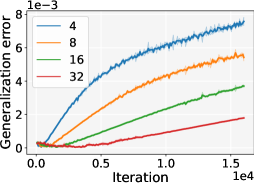
(a) Gen. error of rcv1

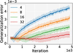
(b) Gen. error of gisette

(c) Gen. error of covtype

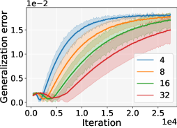
(d) Gen. error of ijcnn1

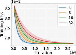
(e) Training loss of ijcnn1

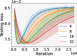
(f) Testing loss of ijcnn1

Figure 4: Supplement to Figure 3. Experimental results for solving quadratic convex problems with delayed SGD. Figures (a) and (b) illustrate the generalization errors with fixed delays, while Figures (c) and (d) show the results for random delays. Figures (e) and (f) depict the training and testing loss of ijcnn1 with random delays. Each experiment was repeated five times, and the variance in the plots is due to selecting different random seeds in multiple trials. The experimental results are consistent with our theoretical findings.

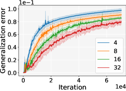
(a) Gen. error of MNIST

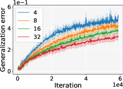
(b) Gen. error of CIFAR-10

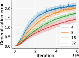
(c) Gen. error of CIFAR-100

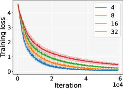
(d) Training loss of CIFAR-100

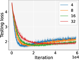
(e) Testing loss of CIFAR-100

Figure 5: Supplement to Figure 1. Experimental result of delayed SGD on three non-convex problems, namely FC+MNIST (Figure (a)), ResNet-18+CIFAR-10 (Figure (b)), and ResNet-18+CIFAR-100 (Figure (c)), with learning rates set to constants of $0.01$, $0.01$ and $0.1$, respectively. Figures (d) and (e) depict the training and testing loss of CIFAR-100. The variance in the plots is due to selecting different random seeds in multiple trials. The non-convex experimental results match well with our theoretical findings for the quadratic problems, suggesting that our theoretical results can be extended to non-convex optimization in some way.

References

• Agarwal and Duchi (2011) Alekh Agarwal and John C Duchi. Distributed delayed stochastic optimization. In J. Shawe-Taylor, R. Zemel, P. Bartlett, F. Pereira, and K.Q. Weinberger, editors, Advances in Neural Information Processing Systems, volume 24. Curran Associates, Inc., 2011.
• Arjevani et al. (2020) Yossi Arjevani, Ohad Shamir, and Nathan Srebro. A tight convergence analysis for stochastic gradient descent with delayed updates. In Aryeh Kontorovich and Gergely Neu, editors, Proceedings of the 31st International Conference on Algorithmic Learning Theory, volume 117, pages 111–132. PMLR, 2020.
• Assran et al. (2020) Mahmoud Assran, Arda Aytekin, Hamid Reza Feyzmahdavian, Mikael Johansson, and Michael G Rabbat. Advances in asynchronous parallel and distributed optimization. Proceedings of the IEEE, 108(11):2013–2031, 2020.
• Aviv et al. (2021) Rotem Zamir Aviv, Ido Hakimi, Assaf Schuster, and Kfir Yehuda Levy. Asynchronous distributed learning: Adapting to gradient delays without prior knowledge. In Marina Meila and Tong Zhang, editors, International Conference on Machine Learning, volume 139, pages 436–445. PMLR, 2021.
• Bäckström et al. (2022) Karl Bäckström, Marina Papatriantafilou, and Philippas Tsigas. ASAP.SGD: Instance-based adaptiveness to staleness in asynchronous SGD. In Kamalika Chaudhuri, Stefanie Jegelka, Le Song, Csaba Szepesvari, Gang Niu, and Sivan Sabato, editors, Proceedings of the 39th International Conference on Machine Learning, volume 162, pages 1261–1276. PMLR, 2022.
• Banerjee et al. (2022) Arindam Banerjee, Tiancong Chen, Xinyan Li, and Yingxue Zhou. Stability based generalization bounds for exponential family langevin dynamics. In Kamalika Chaudhuri, Stefanie Jegelka, Le Song, Csaba Szepesvari, Gang Niu, and Sivan Sabato, editors, International Conference on Machine Learning, volume 162, pages 1412–1449. PMLR, 2022.
• Bassily et al. (2020) Raef Bassily, Vitaly Feldman, Cristóbal Guzmán, and Kunal Talwar. Stability of stochastic gradient descent on nonsmooth convex losses. In H. Larochelle, M. Ranzato, R. Hadsell, M.F. Balcan, and H. Lin, editors, Advances in Neural Information Processing Systems, volume 33, pages 4381–4391. Curran Associates, Inc., 2020.
• Bottou et al. (2018) Léon Bottou, Frank E Curtis, and Jorge Nocedal. Optimization methods for large-scale machine learning. SIAM review, 60(2):223–311, 2018.
• Bousquet and Elisseeff (2002) Olivier Bousquet and André Elisseeff. Stability and generalization. Journal of Machine Learning Research, 2:499–526, 2002.
• Bousquet et al. (2020) Olivier Bousquet, Yegor Klochkov, and Nikita Zhivotovskiy. Sharper bounds for uniformly stable algorithms. In Jacob Abernethy and Shivani Agarwal, editors, Conference on Learning Theory, volume 125, pages 610–626. PMLR, 2020.
• Brown et al. (2020) Tom Brown, Benjamin Mann, Nick Ryder, Melanie Subbiah, Jared D Kaplan, Prafulla Dhariwal, Arvind Neelakantan, Pranav Shyam, Girish Sastry, Amanda Askell, et al. Language models are few-shot learners. In H. Larochelle, M. Ranzato, R. Hadsell, M.F. Balcan, and H. Lin, editors, Advances in Neural Information Processing Systems, volume 33, pages 1877–1901. Curran Associates, Inc., 2020.
• Chandramoorthy et al. (2022) Nisha Chandramoorthy, Andreas Loukas, Khashayar Gatmiry, and Stefanie Jegelka. On the generalization of learning algorithms that do not converge. In S. Koyejo, S. Mohamed, A. Agarwal, D. Belgrave, K. Cho, and A. Oh, editors, Advances in Neural Information Processing Systems, volume 35, pages 34241–34257. Curran Associates, Inc., 2022.
• Chang and Lin (2011) Chih-Chung Chang and Chih-Jen Lin. LIBSVM: A library for support vector machines. ACM Transactions on Intelligent Systems and Technology, 2:27:1–27:27, 2011.
• Charles and Papailiopoulos (2018) Zachary Charles and Dimitris Papailiopoulos. Stability and generalization of learning algorithms that converge to global optima. In Jennifer Dy and Andreas Krause, editors, International Conference on Machine Learning, volume 80, pages 745–754. PMLR, 2018.
• Cohen et al. (2021) Alon Cohen, Amit Daniely, Yoel Drori, Tomer Koren, and Mariano Schain. Asynchronous stochastic optimization robust to arbitrary delays. In M. Ranzato, A. Beygelzimer, Y. Dauphin, P.S. Liang, and J. Wortman Vaughan, editors, Advances in Neural Information Processing Systems, volume 34, pages 9024–9035. Curran Associates, Inc., 2021.
• Dean et al. (2012) Jeffrey Dean, Greg Corrado, Rajat Monga, Kai Chen, Matthieu Devin, Mark Mao, Marc’aurelio Ranzato, Andrew Senior, Paul Tucker, Ke Yang, et al. Large scale distributed deep networks. In F. Pereira, C.J. Burges, L. Bottou, and K.Q. Weinberger, editors, Advances in Neural Information Processing Systems, volume 25, pages 1223–1231. Curran Associates, Inc., 2012.
• Deng et al. (2009) Jia Deng, Wei Dong, Richard Socher, Li-Jia Li, Kai Li, and Li Fei-Fei. Imagenet: A large-scale hierarchical image database. In 2009 IEEE Conference on Computer Vision and Pattern Recognition, pages 248–255. IEEE, 2009.
• Deng et al. (2023) Xiaoge Deng, Tao Sun, Shengwei Li, and Dongsheng Li. Stability-based generalization analysis of the asynchronous decentralized sgd. In Proceedings of the AAAI Conference on Artificial Intelligence, volume 37, pages 7340–7348, 2023.
• Devroye and Wagner (1979a) Luc Devroye and Terry Wagner. Distribution-free inequalities for the deleted and holdout error estimates. IEEE Transactions on Information Theory, 25(2):202–207, 1979a.
• Devroye and Wagner (1979b) Luc Devroye and Terry Wagner. Distribution-free performance bounds with the resubstitution error estimate (corresp.). IEEE Transactions on Information Theory, 25(2):208–210, 1979b.
• Du et al. (2019) Simon S. Du, Xiyu Zhai, Barnabas Poczos, and Aarti Singh. Gradient descent provably optimizes over-parameterized neural networks. In International Conference on Learning Representations, 2019.
• Elisseeff et al. (2005) Andre Elisseeff, Theodoros Evgeniou, Massimiliano Pontil, and Leslie Pack Kaelbing. Stability of randomized learning algorithms. Journal of Machine Learning Research, 6(3):55–79, 2005.
• Farid and Majumdar (2021) Alec Farid and Anirudha Majumdar. Generalization bounds for meta-learning via PAC-Bayes and uniform stability. In M. Ranzato, A. Beygelzimer, Y. Dauphin, P.S. Liang, and J. Wortman Vaughan, editors, Advances in Neural Information Processing Systems, volume 34, pages 2173–2186. Curran Associates, Inc., 2021.
• Farnia and Ozdaglar (2021) Farzan Farnia and Asuman Ozdaglar. Train simultaneously, generalize better: Stability of gradient-based minimax learners. In Marina Meila and Tong Zhang, editors, International Conference on Machine Learning, volume 139, pages 3174–3185. PMLR, 2021.
• Feldman and Vondrak (2018) Vitaly Feldman and Jan Vondrak. Generalization bounds for uniformly stable algorithms. In S. Bengio, H. Wallach, H. Larochelle, K. Grauman, N. Cesa-Bianchi, and R. Garnett, editors, Advances in Neural Information Processing Systems, volume 31. Curran Associates, Inc., 2018.
• Feldman and Vondrak (2019) Vitaly Feldman and Jan Vondrak. High probability generalization bounds for uniformly stable algorithms with nearly optimal rate. In Alina Beygelzimer and Daniel Hsu, editors, Conference on Learning Theory, volume 99, pages 1270–1279. PMLR, 2019.
• Flajolet and Sedgewick (2009) Philippe Flajolet and Robert Sedgewick. Combinatorial structures and ordinary generating functions, page 15–94. Cambridge University Press, 2009.
• Guan et al. (2022) Jiechao Guan, Yong Liu, and Zhiwu Lu. Fine-grained analysis of stability and generalization for modern meta learning algorithms. In S. Koyejo, S. Mohamed, A. Agarwal, D. Belgrave, K. Cho, and A. Oh, editors, Advances in Neural Information Processing Systems, volume 35, pages 18487–18500. Curran Associates, Inc., 2022.
• Hardt et al. (2016) Moritz Hardt, Ben Recht, and Yoram Singer. Train faster, generalize better: Stability of stochastic gradient descent. In Maria Florina Balcan and Kilian Q. Weinberger, editors, International Conference on Machine Learning, volume 48, pages 1225–1234. PMLR, 2016.
• He et al. (2019) Fengxiang He, Tongliang Liu, and Dacheng Tao. Control batch size and learning rate to generalize well: Theoretical and empirical evidence. In H. Wallach, H. Larochelle, A. Beygelzimer, F. d'Alché-Buc, E. Fox, and R. Garnett, editors, Advances in Neural Information Processing Systems, volume 32. Curran Associates, Inc., 2019.
• He et al. (2016) Kaiming He, Xiangyu Zhang, Shaoqing Ren, and Jian Sun. Deep residual learning for image recognition. In IEEE Conference on Computer Vision and Pattern Recognition, pages 770–778, 2016.
• Hsieh et al. (2022) Yu-Guan Hsieh, Franck Iutzeler, Jérôme Malick, and Panayotis Mertikopoulos. Multi-agent online optimization with delays: Asynchronicity, adaptivity, and optimism. Journal of Machine Learning Research, 23(78):1–49, 2022.
• Jacot et al. (2018) Arthur Jacot, Franck Gabriel, and Clément Hongler. Neural tangent kernel: Convergence and generalization in neural networks. In S. Bengio, H. Wallach, H. Larochelle, K. Grauman, N. Cesa-Bianchi, and R. Garnett, editors, Advances in Neural Information Processing Systems, volume 31. Curran Associates, Inc., 2018.
• Koloskova et al. (2022) Anastasiia Koloskova, Sebastian U Stich, and Martin Jaggi. Sharper convergence guarantees for asynchronous SGD for distributed and federated learning. In S. Koyejo, S. Mohamed, A. Agarwal, D. Belgrave, K. Cho, and A. Oh, editors, Advances in Neural Information Processing Systems, volume 35, pages 17202–17215. Curran Associates, Inc., 2022.
• Krizhevsky et al. (2009) Alex Krizhevsky, Geoffrey Hinton, et al. Learning multiple layers of features from tiny images. pages 32–33, 2009.
• Kuzborskij and Lampert (2018) Ilja Kuzborskij and Christoph Lampert. Data-dependent stability of stochastic gradient descent. In Jennifer Dy and Andreas Krause, editors, International Conference on Machine Learning, volume 80, pages 2815–2824. PMLR, 2018.
• LeCun et al. (1998) Yann LeCun, Léon Bottou, Yoshua Bengio, and Patrick Haffner. Gradient-based learning applied to document recognition. Proceedings of the IEEE, 86(11):2278–2324, 1998.
• Lee et al. (2019) Jaehoon Lee, Lechao Xiao, Samuel Schoenholz, Yasaman Bahri, Roman Novak, Jascha Sohl-Dickstein, and Jeffrey Pennington. Wide neural networks of any depth evolve as linear models under gradient descent. In H. Wallach, H. Larochelle, A. Beygelzimer, F. d'Alché-Buc, E. Fox, and R. Garnett, editors, Advances in Neural Information Processing Systems, volume 32. Curran Associates, Inc., 2019.
• Lei and Ying (2020) Yunwen Lei and Yiming Ying. Fine-grained analysis of stability and generalization for stochastic gradient descent. In Hal Daumé III and Aarti Singh, editors, International Conference on Machine Learning, volume 119, pages 5809–5819. PMLR, 2020.
• Lei et al. (2020) Yunwen Lei, Antoine Ledent, and Marius Kloft. Sharper generalization bounds for pairwise learning. In H. Larochelle, M. Ranzato, R. Hadsell, M.F. Balcan, and H. Lin, editors, Advances in Neural Information Processing Systems, volume 33, pages 21236–21246. Curran Associates, Inc., 2020.
• Lei et al. (2021) Yunwen Lei, Zhenhuan Yang, Tianbao Yang, and Yiming Ying. Stability and generalization of stochastic gradient methods for minimax problems. In Marina Meila and Tong Zhang, editors, International Conference on Machine Learning, volume 139, pages 6175–6186. PMLR, 2021.
• Lei et al. (2022) Yunwen Lei, Rong Jin, and Yiming Ying. Stability and generalization analysis of gradient methods for shallow neural networks. In S. Koyejo, S. Mohamed, A. Agarwal, D. Belgrave, K. Cho, and A. Oh, editors, Advances in Neural Information Processing Systems, volume 35, pages 38557–38570. Curran Associates, Inc., 2022.
• Li et al. (2018) Hao Li, Zheng Xu, Gavin Taylor, Christoph Studer, and Tom Goldstein. Visualizing the loss landscape of neural nets. In S. Bengio, H. Wallach, H. Larochelle, K. Grauman, N. Cesa-Bianchi, and R. Garnett, editors, Advances in Neural Information Processing Systems, volume 31. Curran Associates, Inc., 2018.
• Li et al. (2014) Mu Li, David G Andersen, Jun Woo Park, Alexander J Smola, Amr Ahmed, Vanja Josifovski, James Long, Eugene J Shekita, and Bor-Yiing Su. Scaling distributed machine learning with the parameter server. In 11th USENIX Symposium on Operating Systems Design and Implementation (OSDI 14), pages 583–598. USENIX Association, 2014.
• Lian et al. (2015) Xiangru Lian, Yijun Huang, Yuncheng Li, and Ji Liu. Asynchronous parallel stochastic gradient for nonconvex optimization. In C. Cortes, N. Lawrence, D. Lee, M. Sugiyama, and R. Garnett, editors, Advances in Neural Information Processing Systems, volume 28. Curran Associates, Inc., 2015.
• Ma et al. (2018) Siyuan Ma, Raef Bassily, and Mikhail Belkin. The power of interpolation: Understanding the effectiveness of SGD in modern over-parametrized learning. In Jennifer Dy and Andreas Krause, editors, International Conference on Machine Learning, volume 80, pages 3325–3334. PMLR, 2018.
• Mania et al. (2017) Horia Mania, Xinghao Pan, Dimitris Papailiopoulos, Benjamin Recht, Kannan Ramchandran, and Michael I. Jordan. Perturbed iterate analysis for asynchronous stochastic optimization. SIAM Journal on Optimization, 27(4):2202–2229, 2017.
• Mishchenko et al. (2022) Konstantin Mishchenko, Francis Bach, Mathieu Even, and Blake E Woodworth. Asynchronous SGD beats minibatch SGD under arbitrary delays. In S. Koyejo, S. Mohamed, A. Agarwal, D. Belgrave, K. Cho, and A. Oh, editors, Advances in Neural Information Processing Systems, volume 35, pages 420–433. Curran Associates, Inc., 2022.
• Mnih et al. (2016) Volodymyr Mnih, Adria Puigdomenech Badia, Mehdi Mirza, Alex Graves, Timothy Lillicrap, Tim Harley, David Silver, and Koray Kavukcuoglu. Asynchronous methods for deep reinforcement learning. In Maria Florina Balcan and Kilian Q. Weinberger, editors, International conference on machine learning, volume 48, pages 1928–1937. PMLR, 2016.
• Mou et al. (2018) Wenlong Mou, Liwei Wang, Xiyu Zhai, and Kai Zheng. Generalization bounds of SGLD for non-convex learning: Two theoretical viewpoints. In Sébastien Bubeck, Vianney Perchet, and Philippe Rigollet, editors, Conference on Learning Theory, volume 75, pages 605–638. PMLR, 2018.
• Mukherjee et al. (2006) Sayan Mukherjee, Partha Niyogi, Tomaso Poggio, and Ryan Rifkin. Learning theory: stability is sufficient for generalization and necessary and sufficient for consistency of empirical risk minimization. Advances in Computational Mathematics, 25(1-3):161–193, 2006.
• Nedić et al. (2001) Angelia Nedić, Dimitri P Bertsekas, and Vivek S Borkar. Distributed asynchronous incremental subgradient methods. Studies in Computational Mathematics, 8(C):381–407, 2001.
• Ozdaglar et al. (2022) Asuman Ozdaglar, Sarath Pattathil, Jiawei Zhang, and Kaiqing Zhang. What is a good metric to study generalization of minimax learners? In S. Koyejo, S. Mohamed, A. Agarwal, D. Belgrave, K. Cho, and A. Oh, editors, Advances in Neural Information Processing Systems, volume 35, pages 38190–38203. Curran Associates, Inc., 2022.
• Recht et al. (2011) Benjamin Recht, Christopher Re, Stephen Wright, and Feng Niu. Hogwild!: A lock-free approach to parallelizing stochastic gradient descent. In J. Shawe-Taylor, R. Zemel, P. Bartlett, F. Pereira, and K.Q. Weinberger, editors, Advances in Neural Information Processing Systems, volume 24. Curran Associates, Inc., 2011.
• Regatti et al. (2019) Jayanth Regatti, Gaurav Tendolkar, Yi Zhou, Abhishek Gupta, and Yingbin Liang. Distributed SGD generalizes well under asynchrony. In 2019 57th Annual Allerton Conference on Communication, Control, and Computing (Allerton), pages 863–870. IEEE, 2019.
• Ren et al. (2020) Zhaolin Ren, Zhengyuan Zhou, Linhai Qiu, Ajay Deshpande, and Jayant Kalagnanam. Delay-adaptive distributed stochastic optimization. In Proceedings of the AAAI Conference on Artificial Intelligence, volume 34, pages 5503–5510, 2020.
• Richards and Kuzborskij (2021) Dominic Richards and Ilja Kuzborskij. Stability & generalisation of gradient descent for shallow neural networks without the neural tangent kernel. In M. Ranzato, A. Beygelzimer, Y. Dauphin, P.S. Liang, and J. Wortman Vaughan, editors, Advances in Neural Information Processing Systems, volume 34, pages 8609–8621. Curran Associates, Inc., 2021.
• Robbins and Monro (1951) Herbert Robbins and Sutton Monro. A stochastic approximation method. The Annals of Mathematical Statistics, 22(3):400–407, 1951.
• Rogers and Wagner (1978) William H Rogers and Terry J Wagner. A finite sample distribution-free performance bound for local discrimination rules. The Annals of Statistics, 6(3):506–514, 1978.
• Shalev-Shwartz et al. (2010) Shai Shalev-Shwartz, Ohad Shamir, Nathan Srebro, and Karthik Sridharan. Learnability, stability and uniform convergence. Journal of Machine Learning Research, 11(90):2635–2670, 2010.
• Sra et al. (2016) Suvrit Sra, Adams Wei Yu, Mu Li, and Alex Smola. Adadelay: Delay adaptive distributed stochastic optimization. In Arthur Gretton and Christian C. Robert, editors, Artificial Intelligence and Statistics, volume 51, pages 957–965. PMLR, 2016.
• Stanley and Fomin (1999) Richard P. Stanley and Sergey Fomin. Enumerative Combinatorics, volume 2 of Cambridge Studies in Advanced Mathematics. Cambridge University Press, 1999.
• Stich and Karimireddy (2020) Sebastian U Stich and Sai Praneeth Karimireddy. The error-feedback framework: Better rates for SGD with delayed gradients and compressed updates. Journal of Machine Learning Research, 21(237):1–36, 2020.
• Sun et al. (2017) Tao Sun, Robert Hannah, and Wotao Yin. Asynchronous coordinate descent under more realistic assumptions. In I. Guyon, U. Von Luxburg, S. Bengio, H. Wallach, R. Fergus, S. Vishwanathan, and R. Garnett, editors, Advances in Neural Information Processing Systems, volume 30. Curran Associates, Inc., 2017.
• Sun et al. (2021) Tao Sun, Dongsheng Li, and Bao Wang. Stability and generalization of decentralized stochastic gradient descent. In Proceedings of the AAAI Conference on Artificial Intelligence, volume 35, pages 9756–9764, 2021.
• Tsitsiklis et al. (1986) John Tsitsiklis, Dimitri Bertsekas, and Michael Athans. Distributed asynchronous deterministic and stochastic gradient optimization algorithms. IEEE Transactions on Automatic Control, 31(9):803–812, 1986.
• Wilf (1990) Herbert S. Wilf. Chapter 2 - series. In Herbert S. Wilf, editor, Generatingfunctionology, pages 27–63. Academic Press, 1990.
• Wu et al. (2019) Xinxing Wu, Junping Zhang, and Fei-Yue Wang. Stability-based generalization analysis of distributed learning algorithms for big data. IEEE Transactions on Neural Networks and Learning Systems, 31(3):801–812, 2019.
• Xiao et al. (2022) Jiancong Xiao, Yanbo Fan, Ruoyu Sun, Jue Wang, and Zhi-Quan Luo. Stability analysis and generalization bounds of adversarial training. In S. Koyejo, S. Mohamed, A. Agarwal, D. Belgrave, K. Cho, and A. Oh, editors, Advances in Neural Information Processing Systems, volume 35, pages 15446–15459. Curran Associates, Inc., 2022.
• Xing et al. (2021) Yue Xing, Qifan Song, and Guang Cheng. On the algorithmic stability of adversarial training. In M. Ranzato, A. Beygelzimer, Y. Dauphin, P.S. Liang, and J. Wortman Vaughan, editors, Advances in Neural Information Processing Systems, volume 34, pages 26523–26535. Curran Associates, Inc., 2021.
• Yang et al. (2021) Zhenhuan Yang, Yunwen Lei, Puyu Wang, Tianbao Yang, and Yiming Ying. Simple stochastic and online gradient descent algorithms for pairwise learning. In M. Ranzato, A. Beygelzimer, Y. Dauphin, P.S. Liang, and J. Wortman Vaughan, editors, Advances in Neural Information Processing Systems, volume 34, pages 20160–20171. Curran Associates, Inc., 2021.
• Zhang et al. (2017) Chiyuan Zhang, Samy Bengio, Moritz Hardt, Benjamin Recht, and Oriol Vinyals. Understanding deep learning requires rethinking generalization. In International Conference on Learning Representations, 2017.
• Zhang et al. (2016) Wei Zhang, Suyog Gupta, Xiangru Lian, and Ji Liu. Staleness-aware async-SGD for distributed deep learning. In Subbarao Kambhampati, editor, Proceedings of the Twenty-Fifth International Joint Conference on Artificial Intelligence, pages 2350–2356. IJCAI/AAAI Press, 2016.
• Zhang et al. (2022) Yikai Zhang, Wenjia Zhang, Sammy Bald, Vamsi Pingali, Chao Chen, and Mayank Goswami. Stability of SGD: Tightness analysis and improved bounds. In James Cussens and Kun Zhang, editors, Uncertainty in Artificial Intelligence, volume 180, pages 2364–2373. PMLR, 2022.
• Zheng et al. (2017) Shuxin Zheng, Qi Meng, Taifeng Wang, Wei Chen, Nenghai Yu, Zhi-Ming Ma, and Tie-Yan Liu. Asynchronous stochastic gradient descent with delay compensation. In Doina Precup and Yee Whye Teh, editors, International Conference on Machine Learning, volume 70, pages 4120–4129. PMLR, 2017.
• Zhou et al. (2022) Yi Zhou, Yingbin Liang, and Huishuai Zhang. Understanding generalization error of SGD in nonconvex optimization. Machine Learning, 111(1):345–375, 2022.
• Zhou et al. (2018) Zhengyuan Zhou, Panayotis Mertikopoulos, Nicholas Bambos, Peter Glynn, Yinyu Ye, Li-Jia Li, and Li Fei-Fei. Distributed asynchronous optimization with unbounded delays: How slow can you go? In Jennifer Dy and Andreas Krause, editors, International Conference on Machine Learning, volume 80, pages 5970–5979. PMLR, 2018.
• Zhu et al. (2022) Tongtian Zhu, Fengxiang He, Lan Zhang, Zhengyang Niu, Mingli Song, and Dacheng Tao. Topology-aware generalization of decentralized SGD. In Kamalika Chaudhuri, Stefanie Jegelka, Le Song, Csaba Szepesvari, Gang Niu, and Sivan Sabato, editors, International Conference on Machine Learning, volume 162, pages 27479–27503. PMLR, 2022.
• Zinkevich et al. (2010) Martin Zinkevich, Markus Weimer, Lihong Li, and Alex Smola. Parallelized stochastic gradient descent. In J. Lafferty, C. Williams, J. Shawe-Taylor, R. Zemel, and A. Culotta, editors, Advances in Neural Information Processing Systems, volume 23. Curran Associates, Inc., 2010.
• Zou et al. (2021) Difan Zou, Jingfeng Wu, Vladimir Braverman, Quanquan Gu, and Sham Kakade. Benign overfitting of constant-stepsize SGD for linear regression. In Mikhail Belkin and Samory Kpotufe, editors, Proceedings of Thirty Fourth Conference on Learning Theory, volume 134, pages 4633–4635. PMLR, 2021.