MonoNeRD: NeRF-like Representations for Monocular 3D Object Detection

Abstract

In the field of monocular 3D detection, it is common practice to utilize scene geometric clues to enhance the detector’s performance. However, many existing works adopt these clues explicitly such as estimating a depth map and back-projecting it into 3D space. This explicit methodology induces sparsity in 3D representations due to the increased dimensionality from 2D to 3D, and leads to substantial information loss, especially for distant and occluded objects. To alleviate this issue, we propose MonoNeRD, a novel detection framework that can infer dense 3D geometry and occupancy. Specifically, we model scenes with Signed Distance Functions (SDF), facilitating the production of dense 3D representations. We treat these representations as Neural Radiance Fields (NeRF) and then employ volume rendering to recover RGB images and depth maps. To the best of our knowledge, this work is the first to introduce volume rendering for M3D, and demonstrates the potential of implicit reconstruction for image-based 3D perception. Extensive experiments conducted on the KITTI-3D benchmark and Waymo Open Dataset demonstrate the effectiveness of MonoNeRD. Codes are available at https://github.com/cskkxjk/MonoNeRD.

1 Introduction

Monocular 3D detection (M3D) is an active research topic in the computer vision community due to its convenience, low cost and wide range of applications, including autonomous driving, robotic navigation and more. The key point of the task is to establish reasonable correspondences between 2D images and 3D space. Some works leverage geometrical priors to extract 3D information, such as object poses via 2D-3D constraints. These constraints usually require additional keypoint annotations [10, 21] or CAD models [5, 34]. Other works convert estimated depth maps into 3D point cloud representations (Pseudo-LiDAR) [32, 55, 60]. Depth estimates are also used to combine with image features [58, 33] or generate meaningful bird’s-eye-view (BEV) representations [45, 47, 48, 51], then produce 3D object detection results. These methods have made remarkable progress in M3D.

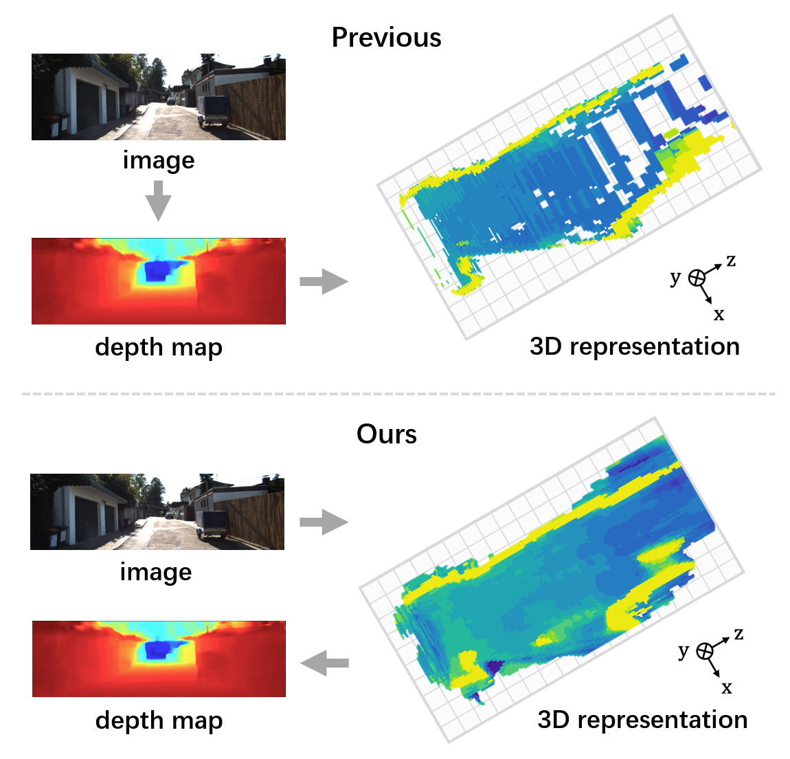
Figure 1: Different intermediate 3D representations. Previous depth-based methods generate 3D representations by back-projecting estimated depth maps to 3D space, whereas our method predicts implicit 3D representations, and obtains depth estimates through volume rendering.

Unfortunately, current 3D representations transformed by explicit depths have some limitations. First, the lifted features obtained from depth estimates or pseudo-LiDAR exhibit an uneven distribution throughout the 3D space. Specifically, they have high density in close range, but the density decreases as the distance increases. (See top part of Figure 1). Second, the final detection performance heavily depends on the accuracy of the depth estimation, which remains challenging to improve. Thus such representations cannot produce dense reasonable 3D features for M3D.

Recent researches in Neural Radiance Fields (NeRF) [3, 38, 64] have shown the capability to reconstruct detailed and dense 3D scene geometry and occupancy information from posed images (images with known camera poses). Inspired by NeRF and its follow-ups [20, 25, 59], we reformulate the intermediate 3D representations in M3D to NeRF-like 3D representations, which can produce dense reasonable 3D geometry and occupancy. To achieve this goal, we combine extracted 2D backbone features and corresponding normalized frustum 3D coordinates to construct 3D Position-aware Frustum features (Section 4.1.1). These 3D features are used to create signed distance fields and radiance fields (RGB color). The signed distance fields encode the distance to the closest surface at every location as a scalar value. This allows us to model scenes implicitly by the zero-level set of the signed distance fields. (Section 3.1). We then adopt volume rendering [35] technique to generate RGB images and depth maps from the signed distance fields and radiance fields (Section 4.1.2), supervising them by original RGB images and LiDAR points (Section 4.2). While the previous depth-based methods generate 3D representations based on predicted depth maps, our method generates depth maps based on 3D representations (Figure 1). It is worth noting that our approach is capable of generating dense 3D occupancy (i.e., volume density) without requiring explicit binary occupancy annotations for individual voxels. Experiments on KITTI [17] 3D benchmark and Waymo Open Dataset [52] show the superiority of our NeRF-like representations in monocular 3D detection.

Our main contributions are threefold:

• We present a novel detection framework, named MonoNeRD, that connects Neural Radiance Fields and monocular 3D detection. It leverages NeRF-like continuous 3D representations to enable accurate 3D perception and understanding from a single image.

• We propose to use volume rendering to directly optimize 3D representations in detection tasks. To the best of our knowledge, our work is the first to introduce volume rendering for 3D detection tasks.

• Extensive experiments on KITTI [17] 3D detection benchmark and Waymo Open Dataset [52] demonstrate the effectiveness of our method, which is competitive with previous state-of-the-art works. This research presents the potential of 3D implicit reconstruction for image-based 3D perception.

2 Related Work

2.1 Monocular 3D Object Detection

Many impressive researches [47, 9, 43] been done in monocular 3D object detection. As the essential information of depth dimension is collapsed in the 2D image, it is an ill-posed but necessary problem of finding an approach to lift the 2D information to 3D space.

Some Monocular 3D Object Detection methods lift 2D to 3D directly by incorporating the geometric relationship between the 2D image plane and 3D space. For example, many methods assume rigidity of objects, aligning 2D keypoints with their 3D counterparts [1, 2, 21, 46]. Some researchers try to build the bridge between 2D and 3D structures by template matching [5, 34]. These methods usually require additional data (e.g., 3D CAD models, object keypoint annotations).

Other methods generate intermediate 3D representations to solve the lifting problem. Many approaches [60, 33, 32] convert the estimated depth map (always predicted by an off-the-shelf model) to pseudo-LiDAR point cloud representations, and then feed them to sophisticated LiDAR-based detectors. CaDDN [47] learns categorical depth distributions over pixels to lift camera images into 3D space, constructing BEV representations. Pseudo-Stereo [12] uses some sophisticated modules (e.g., stereo cost volume) to achieve better depth estimation. These methods typically involve estimating depth maps beforehand and subsequently extracting corresponding 3D representations from them. Instead, our method recovers depth maps from the 3D representations and supervises them to improve the detection performance.

2.2 Neural Implicit Representations

Representing 3D geometry with implicit functions has gained popularity in the past few years. Learning-based 3D reconstruction methods [13, 18, 36, 37, 41, 49] and their scene-level counterparts [6, 15, 23, 44] demonstrate compelling results but require 3D input and supervision. Neural Radiance Fields (NeRFs) [38] introduce a new perspective to learn continuous geometry representations from posed multi-view images only by volume rendering [35]. Due to the low efficiency of original MLP-based NeRF, their grid-based variants [22, 28, 61, 7] have been explored to accelerate the rendering process or save GPU memory. To circumvent the requirement of dense inputs, some works [62, 8, 14, 39] explicitly consider sparse input scenarios and show astonishing results for novel view synthesis, but these representations still need to be optimized per scene. Li et al. [25] propose MINE in which they combine Multiplane Images (MPI) and NeRF for single-image-based novel view synthesis. SceneRF [4] uses posed image sequences for training, alleviating the reliance on datasets. Wimbauer et al. [57] construct a density field to preform both depth prediction and novel view synthesis. Unlike our approach, the works mentioned primarily focus on the Novel View Synthesis task, requiring multi-view or sequenced images with camera poses as supervision, which cannot generalize to unseen scenes (except [25, 57]). Instead, we take advantage of volume rendering to optimize 3D feature representations and improve the performance in M3D task.

3 Preliminaries

Here we introduce some essential preliminaries for our idea. We use the same notation as [59] for the concepts of SDF and Volume density. Concerning the space limitation, here we provide a brief overview. Please refer to [38, 59, 35] for more details.

3.1 Signed Distance Function (SDF)

For a given spatial point, Signed Distance Function (SDF) is a continuous function that outputs the point’s distance to the closest surface, whose sign indicates whether the point is inside (negative) or outside (positive) of the surface.

Let $\mathbb{R}^{3}$ represent a 3D space containing some objects, $\Omega\subset\mathbb{R}^{3}$ refers to the occupied part, and $\mathcal{M}=\partial\Omega$ be the boundary surface. Denote the $\Omega$ indicator function by $\mathbf{1}_{\Omega}$, and the Signed Distance Function (SDF) by $d_{\Omega}$,

$$\mathbf{1}_{\Omega}(\bm{x})=\begin{cases}1&\text{if }\bm{x}\in\Omega\\ 0&\text{if }\bm{x}\notin\Omega\end{cases}$$ (1)

$$d_{\Omega}(\bm{x})=(-1)^{\mathbf{1}_{\Omega}(\bm{x})}\min_{\bm{y}\in\mathcal{M}}\left\|\bm{x}-\bm{y}\right\|$$ (2)

where $\left\|{\cdot}\right\|$ is the standard Euclidean 2-norm. The underlying surface $\mathcal{M}$ can be implicitly represented by the zero-level set of $d_{\Omega}({\cdot})=0$.

3.2 Transform SDF to Density

The volume density $\sigma:\mathbb{R}^{3}\rightarrow\mathbb{R}_{+}$ is a scalar volumetric function, where $\sigma(\bm{x})$ can be interpreted as the probability that light is occluded at point $\bm{x}$. Previous works et al. [59, 63] suggest modeling the density $\sigma$ using a certain transformation of a learnable Signed Distance Function (SDF), as follows:

$$\sigma(\bm{x})=\alpha\Psi_{\beta}({-d_{\Omega}(\bm{x})})$$ (3)

where $\alpha,\beta>0$ are learnable parameters and $\Psi_{\beta}$ is the cumulative distribution function of the Laplace distribution with zero mean and $\beta$ scale,

$$\Psi_{\beta}(s)=\begin{cases}\frac{1}{2}\exp({\frac{s}{\beta}})&\text{if }s\leq 0\\ 1-\frac{1}{2}\exp({-\frac{s}{\beta}})&\text{if }s>0\end{cases}$$ (4)

As $\beta$ approaches zero, the density $\sigma$ converges to scaled indicator function of $\Omega$, means $\sigma\rightarrow\alpha\mathbf{1}_{\Omega}$ for all points $\bm{x}\in\Omega\setminus\mathcal{M}$. The benefits of modeling density in this way have been discussed in [59]. We simply set $\alpha=\beta^{-1}$ in our implementations. Figure 2 depicts an example of how density varies along SDF when a ray passes through an object.

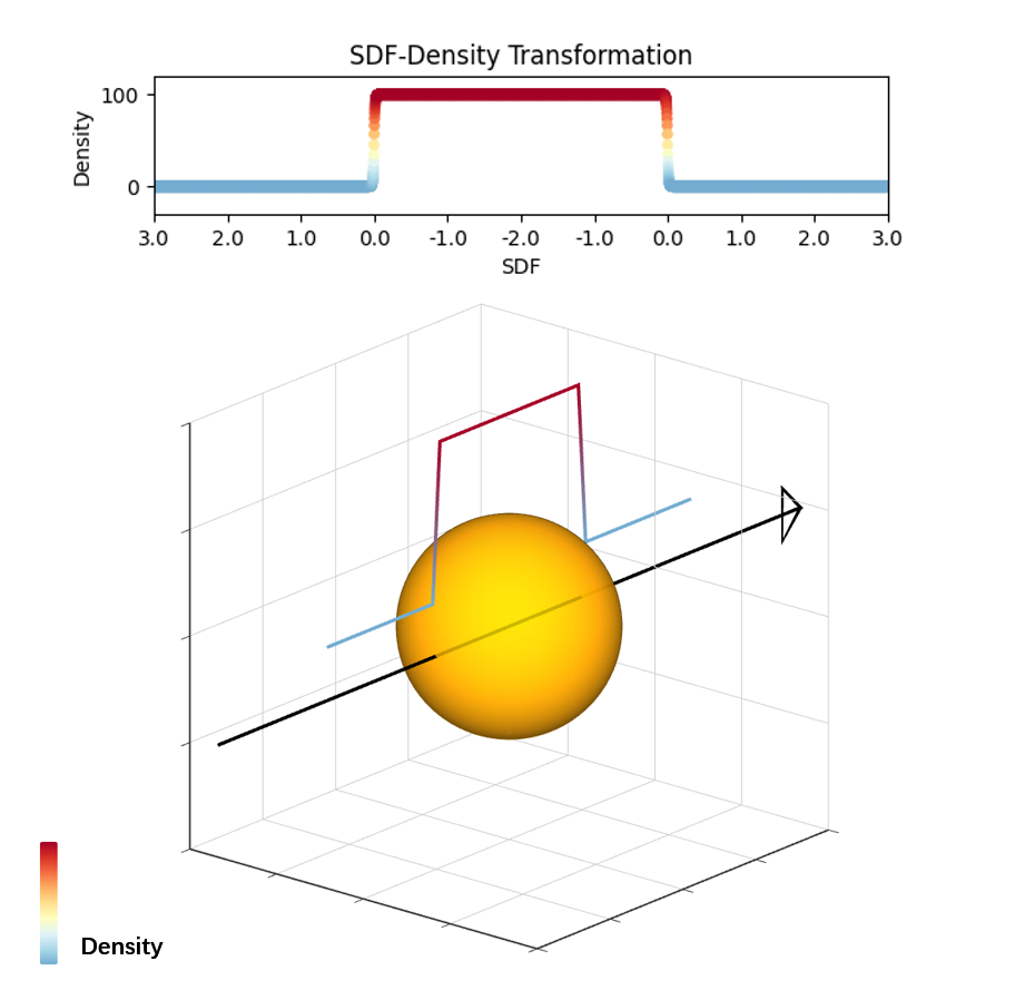
Figure 2: Example of transformation from SDF to Density. The black arrow line represents a ray passing through a spherical object; the gradient color line describes how density varies along with SDF values by Equation 3, where we set $\beta=0.01,\alpha=\beta^{-1}=100$.

3.3 Volume Rendering

Volume intensity (RGB color) $\bm{c}:\mathbb{R}^{3}\rightarrow\mathbb{R}^{3}$ is a vector volumetric function of spatial position $\bm{x}$, where $\bm{c}(x)$ represents the intensity or color at a certain point $\bm{x}$. Given color $c$ and density $\sigma$, the expected color $\bm{C}(\bm{r})$ of ray $\bm{r}(t)=\bm{o}+t\bm{d}$ (where $\bm{o}$ and $\bm{d}$ are the origin and direction of the ray respectively) with near and far bounds $t_{n}$ and $t_{f}$ is:

$$\begin{split}&\bm{C}(\bm{r})=\int_{t_{n}}^{t_{f}}\bm{T}(t)\sigma(\bm{r}(t))\bm{c}(\bm{r}(t))dt,\\ &\text{where }\bm{T}(t)=\exp\left(-\int_{t_{n}}^{t}\sigma(\bm{r}(s))ds\right)\end{split}$$ (5)

where $\sigma$ refers to the volume density. The function $\bm{T}(t)$ denotes the accumulated transmittance along the ray from $t_{n}$ to $t$, namely, the probability that the ray (or light) travels from $t_{n}$ to $t$ without being occluded by any particle. In Section 4.1.2, we describe the details to calculate volume rendering numerical integration in our setup.

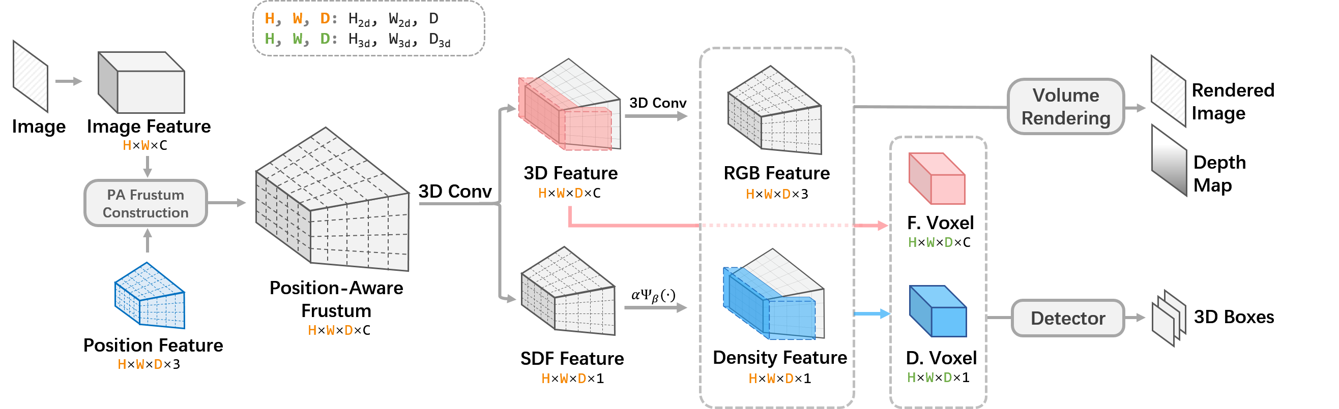
Figure 3: Overview of MonoNeRD. “F. Voxel” and “D. Voxel” in the figure refer to Feature Voxel and Density Voxel, respectively. Position-Aware Frustum Features $F_{P}$ are generated from an image $I$ and Positional Frustum Features $F_{pos}$ in a query-based manner (Section 4.1.1), which are then transformed to 3D features $F^{\prime\prime}$ and signed distance fields $F_{sdf}$. After that, the radiance fields $F_{rgb}$ are produced by $F^{\prime\prime}$ (Section 4.1.2). $F_{sdf}$ can be transformed to frustum volume density $F_{density}$ (Equation 3) by a scaled cumulative distribution function of Laplace distribution (Equation 4). Volume rendering from $F_{rgb}$ and $F_{density}$ provides supervision for such NeRF-like representations which generate voxel features $V_{3d}$ for M3D (Section 4.1.3).

4 Method

Overview. The overall framework is illustrated in Figure 3. We follow the network design in LIGA-Stereo [19]. Note that the stereo part of LIGA-Stereo [19] is not applicable for monocular 3D detection (M3D) task. We replace the intermediate 3D feature representations with the proposed NeRF-like representations while keeping the 2D image backbone and downstream detection module unchanged.

Given an input RGB image $I\in\mathbb{R}^{H\times W\times 3}$, it is passed to a 2D image backbone for extracting image features. Then we use the 2D image features to generate the proposed NeRF-like 3D representations. Specifically, we first build the Position-aware Frustum (See Section 4.1.1), which is transformed to 3D frustum features and SDF frustum features. Such features can be used for obtaining RGB and density features to achieve rendered RGB images and depth maps via Volume Rendering (See Section 4.1.2). They are supervised by RGB loss and depth loss to guide previous features, serving as auxiliary tasks in training. Furthermore, we use grid-sampling on 3D frustum features and density frustum features to build regular 3D voxel features and corresponding density. They are used for forming 3D Voxel Features (See Section 4.1.3), which are fed into the detection modules. We elaborate on each part of our method in the following.

4.1 NeRF-like Representation

We need to clarify the difference between NeRF and the proposed NeRF-like representation. NeRF encodes a scene with a MLP and has to be trained per scene. The proposed method predicts continuous 3D geometry information from the single input RGB image. Similar ideas have been explored in researches about single-image-based novel view synthesis. Please refer to [20, 25] for details.

4.1.1 Position-aware Frustum Construction

To lift 2D backbone features to 3D space without depth, a naive manner is to simply repeat 2D features on different depth planes. However, this way does not contain any position information, causing ambiguous spatial features. To resolve this problem, we propose to generate position-aware frustum features.

Taking an RGB image as input, the 2D image backbone produces image features $F_{image}\in\mathbb{R}^{H_{2d}\times W_{2d}\times C}$, where $H_{2d}\text{ and }W_{2d}$ are the height and width of the 2D image feature map, and $C$ is the number of feature channels. Such 2D image features are mapped to a camera frustum along with corresponding normalized frustum 3D coordinates in a query-based manner. More specifically, given pre-defined near depth $z_{n}$ and far depth $z_{f}$, we sample $D$ planes from this depth range under equal depth intervals with random perturbation as described in [38, 25]. Each depth plane consists of frustum 3D position coordinates $p:[u,v,z]^{T}$ of every pixel point $[u,v]^{T}\in\mathbb{R}^{2}$. These coordinates are normalized later. Thus we have 3D positional frustum features $F_{pos}\in\mathbb{R}^{H_{2d}\times W_{2d}\times D\times 3}$, where $D$ refers to the number of depth planes and $3$ denotes the normalized coordinates. To combine 3D position and original 2D image features, we use three linear layers $f_{q},f_{k},f_{v}$ to do the Query-Key-Value mapping and attention calculation (in Figure 4).

$$\begin{split}&f_{q}:F_{pos}\rightarrow Q\in\mathbb{R}^{H_{2d}\times W_{2d}\times D\times C}\\ &f_{k}:F_{image}\rightarrow K\in\mathbb{R}^{H_{2d}\times W_{2d}\times C}\\ &f_{v}:F_{image}\rightarrow V\in\mathbb{R}^{H_{2d}\times W_{2d}\times C}\end{split}$$ (6)

Therefore, the Position-Aware Frustum features can be calculated by a softmax function along the depth dimension.

$$F_{P}=\text{Softmax}(QK\text{, dim=D})V$$ (7)

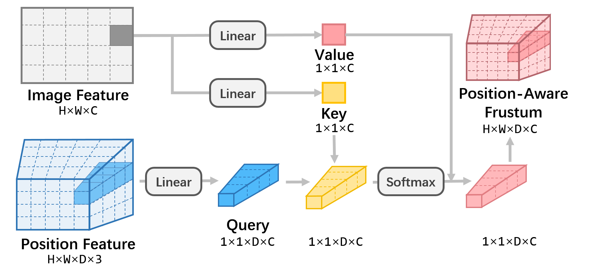
Figure 4: The Query-Key-Value mapping procedure for constructing Position-Aware Frustum features.

4.1.2 Volume Rendering within Frustum

After constructing position-aware frustum features, we try to encode such features in 3D space to obtain more informative 3D features for volume rendering. Towards this goal, we employ two 3D convolution blocks $f_{1}$ and $f_{2}$. $f_{1}$ consists of a three-layer 3D-convolution with kernel size 3 and softplus activation. It takes position-aware frustum features $F_{P}\in\mathbb{R}^{H_{2d}\times W_{2d}\times D\times C}$ as input, outputting a same shape feature $F^{\prime}$ except the channel number, as follows:

$$f_{1}:F_{P}\rightarrow F^{\prime}\in\mathbb{R}^{H_{2d}\times W_{2d}\times D\times\left(1+C\right)}$$ (8)

i) SDF and density features. The first channel feature in $F^{\prime}$ is regarded as SDF feature $F_{sdf}\in\mathbb{R}^{H_{2d}\times W_{2d}\times D\times 1}$. The signed distance fields $F_{sdf}$ represent the scene geometry of the input image. For any 3D point $[x,y,z]^{T}$ in frustum space, we can get its signed distance $s(x,y,z)\in\mathbb{R}^{1}$ by trilinear sampling in $F_{sdf}$. Furthermore, scene volume density $\sigma$ (or density frustum $F_{density}\in\mathbb{R}^{H_{2d}\times W_{2d}\times D\times 1}$) can be transformed by Equation 3:

$$\begin{split}&\sigma(x,y,z)=\alpha\Psi_{\beta}({s(x,y,z)})\\ &F_{density}=\alpha\Psi_{\beta}(F_{sdf})\end{split}$$ (9)

The density will be used for rendering depth maps and weighing the voxel features.

ii) RGB features. The remaining $C$ channel feature in $F^{\prime}$, called $F^{\prime\prime}$, is then passed to $f_{2}$, which consists of a one-layer 3D-convolution with kernel size 3 and sigmoid activation.

$$f_{2}:F^{\prime\prime}\rightarrow F_{rgb}\in\mathbb{R}^{H_{2d}\times W_{2d}\times D\times 3}$$ (10)

The resulting feature is used for approximating the scene radiance field $F_{rgb}$. We can also get color intensity $c(x,y,z)\in\mathbb{R}^{3}$ by trilinear sampling in $F_{rgb}$.

Rendering from original view. To save GPU memory, we render downsampled RGB image $\hat{I}_{low}$ and depth map $\hat{Z}_{low}$. According to known camera calibration and multiple depth value $\{z_{i}|i=1,...,D\}$, a pixel point $[u,v]^{T}$ in $\hat{I}$ can be back-projected to several 3D point coordinates $\{[x_{i},y_{i},z_{i}]^{T}|i=1,...,D\}$. We can calculate the distance between two successive 3D points as follows:

$$\delta_{x_{i},y_{i},z_{i}}=\left\|{[x_{i+1},y_{i+1},z_{i+1}]^{T}-[x_{i},y_{i},z_{i}]^{T}}\right\|_{2}$$ (11)

Denote the distance map at depth $z_{i}$ as $\delta_{z_{i}}\in\mathbb{R}^{H_{2d}\times W_{2d}\times 1}$, we can easily get the density map $\sigma_{z_{i}}\in\mathbb{R}^{H_{2d}\times W_{2d}\times 1}$ from $F_{density}$ and color map $c_{z_{i}}\in\mathbb{R}^{H_{2d}\times W_{2d}\times 3}$ from $F_{rgb}$. Then we can render $\hat{I}$ by:

$$\begin{split}&\hat{I}_{low}=\sum_{i=1}^{D}T_{i}(1-\text{exp}(-\sigma_{z_{i}}\delta_{z_{i}}))c_{z_{i}},\\ \end{split}$$ (12)

where $T_{i}=\text{exp}\left(-\sum_{j=1}^{i-1}\sigma_{z_{j}}\delta_{z_{j}}\right)$ denotes the accumulated transmittance map from plane 1 to plane $i$. Similarly, the low resolution depth map $\hat{Z}_{low}\in\mathbb{R}^{H_{2d}\times W_{2d}\times 1}$ can be rendered by:

$$\hat{Z}_{low}(u,v)=\sum_{i=1}^{D}T_{i}(1-\text{exp}(-\sigma_{z_{i}}\delta_{z_{i}}))z_{i}$$ (13)

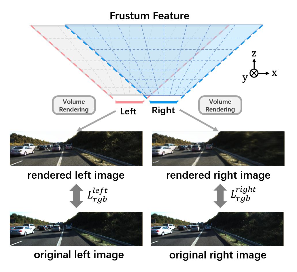
Figure 5: Supervision from two RGB images by using volume rendering. We can obtain associated rendered RGB images from frustum density features $F_{density}$ and frustum radiance fields $F_{rgb}$ via Equation 12. Under this setting, we do not require explicit depth labels (i.e., LiDAR depths). Instead, the depth can be implicitly learned by calculating RGB reconstruction loss between original and rendered images.

We simply upsample $\hat{I}_{low}$ and $\hat{Z}_{low}$ to original image resolution to get target image $\hat{I}\in\mathbb{R}^{H\times W\times 3}$ and depth map $\hat{Z}\in\mathbb{R}^{H\times W\times 1}$. Such recovered RGB images and depth maps will be supervised by RGB loss and depth loss (See Section 4.2). They are used in training as auxiliary tasks to facilitate the learning process and can be discarded at the inference stage.

Rendering from other views. Moreover, we can render from other views as long as such views’ frustum overlaps with the original view’s frustum and their camera calibrations are available. The rendered images can be produced in the same way described above. By calculating the image reconstruction loss from other views’ rendered images, our NeRF-like representations can get extra supervisions. In Figure 5, we give an example of taking the stereo images (left and right images) in KITTI [17] as volume rendering targets. In this way, we can even eliminate the reliance on explicit depth supervisions. Considering the space limitation of the main text, we provided ablation of depth supervision in this supplementary material.

4.1.3 Voxel Features Generation

Aforementioned frustum features cannot be directly used for downstream detection modules as they are irregular in 3D space. Therefore, we must transform 3D frustum features to regular 3D voxel features. We perform this process of converting frustum to voxel just like CaDDN [47] by leveraging camera calibration and differentiable sampling. First, we define a voxel grid $V\in\mathbb{R}^{H_{3d}\times W_{3d}\times D_{3d}\times 3}$, the sampling points $s_{k}^{v}=[x,y,z]_{k}^{T}$ are the center of each voxel. We can transform $s_{k}^{v}$ to get corresponding frustum sampling points $s_{k}^{f}=[u,v,d]_{k}^{T}$ according to the camera calibration matrix. Frustum features ($F^{\prime\prime},F_{density}$) are sampled using sampling points $s_{k}^{f}$ with trilinear interpolation to inhabit voxel features ($V^{\prime\prime},V_{density}$). Different from [47], the spatial resolutions of the frustum grid and voxel grid are not required to be similar because $F_{sdf}$ and $F_{rgb}$ are not limited by spatial resolution.

Considering that the density indicates 3D occupancy in the 3D space, we use it to enhance sampled 3D voxel features $V^{\prime\prime}$. Specifically, we obtain the final 3D voxel features by:

$$V_{3d}=V^{\prime\prime}\cdot\tanh(V_{density})$$ (14)

where $\tanh(\cdot)$ is used to scale $V_{density}$ to the range of $[0,1]$. $V_{3d}$ is a NeRF-like representation since it is optimized in the same way as NeRF to learn the implicit scene geometry and occupancy.

4.2 Loss Function

Equation 12 and 13 build connections between 3D scene representation and 2D observations (i.e., texture and depth). We can therefore optimize the 3D representations with raw 2D RGB images and depth maps. Based on this, there are four terms in the loss function: RGB loss $L_{rgb}$, depth loss $L_{depth}$, SDF loss $L_{sdf}$, and the original loss in the baseline framework LIGA [19] $L_{\text{LIGA}}$. The overall loss is formulated as:

$$L=\lambda_{rgb}L_{rgb}+\lambda_{depth}L_{depth}+\lambda_{sdf}L_{sdf}+\lambda_{\text{LIGA}}L_{\text{LIGA}},$$ (15)

where $\lambda_{rgb},\lambda_{depth},\lambda_{sdf},\lambda_{\text{LIGA}}$ are fixed loss weights. We empirically set all weights to 1 by default.

RGB loss. The RGB loss consists of two items: Smooth L1 loss $L_{\text{smoothL1}}$ and SSIM [56] loss $L_{\text{SSIM}}$ which are usually used in image reconstruction:

$$\begin{split}&L_{rgb}=\lambda_{\text{smoothL1}}L_{\text{smoothL1}}+\lambda_{\text{SSIM}}L_{\text{SSIM}}\\ \end{split}$$ (16)

Depth loss. Depth map labels are obtained by projecting associated LiDAR points onto the image plane. The depth loss is L1 loss between ground truth sparse depth map $Z$ and predicted depth map $\hat{Z}$,

$$L_{depth}=\frac{1}{N_{depth}}\sum_{u,v}\left\|\hat{Z}-Z\right\|_{1}\\$$ (17)

where $N_{depth}$ denotes the number of valid pixels $(u,v)$ with LiDAR depth.

SDF loss. The SDF loss encourages $F_{sdf}$ to vanish on geometry surface $\mathcal{M}$,

$$L_{sdf}=\frac{1}{N_{gt}}\sum_{x,y,z}(\left\|F_{sdf}(x,y,z)\right\|_{2})$$ (18)

where $N_{gt}$ denotes the number of LiDAR points in the current camera view.

LIGA loss We denote the original loss in LIGA [19] as $L_{\text{LIGA}}$. We keep the detection, imitation and auxiliary 2D supervision loss items but remove the stereo depth estimation item to fit the monocular setting. The imitation item is removed in all Waymo [52] experiments for convenience.

$$\begin{split}&L_{\text{LIGA-KITTI}}=L_{\text{det}}+\lambda_{im}L_{im}+\lambda_{2d}L_{2d}\\ &L_{\text{LIGA-Waymo}}=L_{\text{det}}+\lambda_{2d}L_{2d}\end{split}$$ (19)

Methods	Reference	Category	$AP_{BEV}$			$AP_{3D}$
			Easy	Moderate	Hard	Easy	Moderate	Hard
D4LCN[16]	CVPR20	Pretained Depth	22.51	16.02	12.55	16.65	11.72	9.51
DDMP-3D[53]	CVPR21		28.08	17.89	13.44	19.71	12.78	9.80
Ground-Aware[29]	RAL21	Directly Regress	29.81	17.98	13.08	21.65	13.25	9.91
MonoRCNN[50]	ICCV21		25.48	18.11	14.10	18.36	12.65	10.03
MonoEF[66]	CVPR21		29.03	19.70	17.26	21.29	13.87	11.71
MonoRUn[9]	CVPR21	Geometric-based	27.94	17.34	15.24	19.65	12.30	10.58
GUPNet[31]	ICCV21		30.29	21.19	18.20	22.26	15.02	13.12
MonoFlex[65]	CVPR21		28.23	19.75	16.89	19.94	13.89	12.07
DCD[26]	ECCV22		32.55	21.50	18.25	23.81	15.90	13.21
CaDDN[47]	CVPR21	LiDAR Auxiliary	27.94	18.91	17.19	19.17	13.41	11.46
DD3D[40]	ICCV21		30.98	22.56	20.03	23.22	16.34	14.20
DID-M3D[43]	ECCV22		32.95	22.76	19.83	24.40	16.29	13.75
MonoNeRD (ours)	–		31.13	23.46	20.97	22.75	17.13	15.63

Table 1: Comparisons for Car category on KITTI test at IOU threshold 0.7. We obtain the values of other methods from respective papers. We use red to indicate the highest result and blue for the second-highest result. We can see that our method sets a new state of the art.

5 Experiments

5.1 Dataset and Metrics

KITTI. The KITTI dataset [17] comprises of 7,481 images in the training (trainval set) and 7,518 images in the testing (test set) with synchronized LiDAR point clouds. In previous works [11], the training images were split into a train set (3,712 samples) and a val set (3,769 samples). We also follow this setting. Results on the KITTI dataset [17] are measured using IoU-based criteria with a threshold of 0.7 to compute averaged precision over 40 recall values ($AP|_{R40}$) for the car class in both bird’s-eye-view (BEV) and 3D tasks.

Waymo. The Waymo Open Dataset [52] consists of 798 training sequences and 202 validation sequences. We follow the setting in CaDDN [47] which only considers the front camera and uses the sampled training set (51,564 samples). Results on Waymo val are measured by officially evaluation of the mean average precision (mAP) and the mean average precision weighted by heading (mAPH) with IoU criteria of 0.7 and 0.5. The evaluation is performed on two difficulty levels (Level_1 and Level_2) and three distance ranges (0 - 30m, 30m - 50m, 50m - $\infty$).

5.2 Implementation Details

Training details. Our method is implemented with Pytorch [42] framework. We have done all experiments with four NVIDIA 3080Ti (12G) GPUs. The detector is trained using AdamW [30] optimizer with $\beta_{1}=0.9,\beta_{2}=0.999$. The batch size is fixed to 4, with 1 sample on each GPU. On KITTI [17], the input size is fixed to $320\times 1248$, we train 50 epochs using an initial learning rate of 0.001, and 10 epochs with a reduced learning rate of 0.0001, weight decay is 0.0001. On Waymo [52], the input size is fixed to $640\times 960$, we train 16 epochs using an initial learning rate of 0.001, and 4 epochs with a reduced learning rate of 0.0001, weight decay is 0.0001.

Hyperparameters. On KITTI [17], we sample $D=72$ planes within depth range $[z_{n},z_{f}]=[2,59.6](meter)$ in the frustum space. The voxel grid range is $[2,59.6]\times[-30.4,30.4]\times[-3,1](meter)$ and voxel size is $[0.2,0.2,0.2](meter)$ for the depth, width, and height axis in 3D space, respectively. On Waymo [52] the voxel grid range is $[2,59.6]\times[-25.6,25.6]\times[-3,1](meter)$ while all other hypeparameters are the same as KITTI experiments.

5.3 Main Results

KITTI. Table 1 shows the main results of MonoNeRD on the KITTI test set. Our method is competitive with previous methods without any extra data. MonoNeRD achieves the best results under the Moderate and Hard settings in both $AP_{BEV}$ and $AP_{3D}$. Compared to DD3D [40], which uses a vast private dataset for depth pre-training, we boost the performance from 22.56/16.34 to 23.46/17.13 under moderate setting, and from 20.03/14.20 to 20.97/15.63 under hard setting for $AP_{BEV}/AP_{3D}$, respectively. As for DID-M3D [43], we exceed it on both moderate and hard settings with 0.7/1.14 $AP_{BEV}$ and 0.84/1.88 $AP_{3D}$.

Waymo. Table 2 shows the main results of on the Waymo val set. MonoNeRD achieves competitive results without using data augmentation techniques. It has a lightweight backbone (ResNet34) compared to other depth-based methods like CaDDN (ResNet101) and DID-M3D (DLA34).

The Results on both KITTI [17] hard and Waymo [52] distance ranges (30m - 50m, 50m - $\infty$) demonstrate the superiority of our method in handling distant and occluded objects.

5.4 Ablation Studies

Methods	3D mAP / mAPH (IoU = 0.7)				3D mAP / mAPH (IoU = 0.5)
	Overall	0 - 30m	30 - 50m	50m - $\infty$	Overall	0 - 30m	30 - 50m	50m - $\infty$
LEVEL 1
PatchNet [32]	0.39 / 0.37	1.67 / 1.63	0.13 / 0.12	0.03 / 0.03	2.92 / 2.74	10.03 / 9.75	1.09 / 0.96	0.23 / 0.18
CaDDN [47]	5.03 / 4.99	14.54 / 14.43	1.47 / 1.45	0.10 / 0.10	17.54 / 17.31	45.00 / 44.46	9.24 / 9.11	0.64 / 0.62
PCT [54]	0.89 / 0.88	3.18 / 3.15	0.27 / 0.27	0.07 / 0.07	4.20 / 4.15	14.70 / 14.54	1.78 / 1.75	0.39 / 0.39
MonoJSG [27]	0.97 / 0.95	4.65 / 4.59	0.55 / 0.53	0.10 / 0.09	5.65 / 5.47	20.86 / 20.26	3.91 / 3.79	0.97 / 0.92
DEVIANT [24]	2.69 / 2.67	6.95 / 6.90	0.99 / 0.98	0.02 / 0.02	10.98 / 10.89	26.85 / 26.64	5.13 / 5.08	0.18 / 0.18
DID-M3D [43]	- / -	- / -	- / -	- / -	20.66 / 20.47	40.92 / 40.60	15.63 / 15.48	5.35 / 5.24
MonoNeRD (ours)	10.66 / 10.56	27.84 / 27.57	5.40 / 5.36	0.72 / 0.71	31.18 / 30.70	61.11 / 60.28	26.08 / 25.71	6.60 / 6.47
LEVEL 2
PatchNet [32]	0.38 / 0.36	1.67 / 1.63	0.13 / 0.11	0.03 / 0.03	2.42 / 2.28	10.01 / 9.73	1.07 / 0.94	0.22 / 0.16
CaDDN [47]	4.49 / 4.45	14.50 / 14.38	1.42 / 1.41	0.09 / 0.09	16.51 / 16.28	44.87 / 44.33	8.99 / 8.86	0.58 / 0.55
PCT [54]	0.66 / 0.66	3.18 / 3.15	0.27 / 0.26	0.07 / 0.07	4.03 / 3.99	14.67 / 14.51	1.74 / 1.71	0.36 / 0.35
MonoJSG [27]	0.91 / 0.89	4.64 / 4.65	0.55 / 0.53	0.09 / 0.09	5.34 / 5.17	20.79 / 20.19	3.79 / 3.67	0.85 / 0.82
DEVIANT [24]	2.52 / 2.50	6.93 / 6.87	0.95 / 0.94	0.02 / 0.02	10.29 / 10.20	26.75 / 26.54	4.95 / 4.90	0.16 / 0.16
DID-M3D [43]	- / -	- / -	- / -	- / -	19.37 / 19.19	40.77 / 40.46	15.18 / 15.04	4.69 / 4.59
MonoNeRD (ours)	10.03 / 9.93	27.75 / 27.48	5.25 / 5.21	0.60 / 0.59	29.29 / 28.84	60.91 / 60.08	25.36 / 25.00	5.77 / 5.66

Table 2: Results on Waymo val set. We obtain the values of other methods from their respective papers. Our method performs the best.

Architectural components. We conduct an ablation study on the car category in KITTI val to analyze the effectiveness of the proposed NeRF-like representations. In Table 3, Exp. (a) is the baseline which directly takes features sampled from $F_{P}$ as voxel representations $V_{3d}$ for M3D. In Exp. (b), we use more 3D convolution layers to prevent enhancements from complex model structures. Exp. (c) shows that supervision only from a single RGB image is useless and even harmful for detection since a purely single image cannot provide depth information. We can see that sparse depth map labels from LiDAR can significantly improve the performance of the detector from Exp. (d). The effectiveness of $L_{rgb}$ can be revealed by comparing Exp. (d, e) or Exp. (f, g). Finally, SDF loss brings noticeable performance gains, especially on $AP_{BEV}$.

Exp.	Setting				$AP_{BEV}/AP_{3D}$
	3D Conv.	$L_{rgb}$	$L_{depth}$	$L_{sdf}$	Easy	Moderate	Hard
(a)					24.96 / 17.01	19.27 / 13.38	16.89 / 11.73
(b)	✓				25.64 / 17.22	19.75 / 13.65	18.01 / 11.99
(c)	✓	✓			24.83 / 16.92	19.10 / 13.11	16.74 / 11.73
(d)	✓		✓		26.91 / 18.72	20.87 / 14.54	18.57 / 12.60
(e)	✓	✓	✓		26.46 / 19.44	20.16 / 15.03	17.59 / 12.83
(f)	✓		✓	✓	27.94 / 20.28	21.44 / 15.32	18.82 / 13.48
(g)	✓	✓	✓	✓	29.03 / 20.64	22.03 / 15.44	19.41 / 13.99

Table 3: Ablation of network structure and volume rendering loss. “3D Conv.”: 3D convolution blocks as mentioned in Section 4.1.2; “$L_{\left(\cdot\right)}$”: use the loss for supervision; “Exp.”: Experiment.

Positional aware module. Based on experiment (g) in Table 3, we replace the query-key-value (QKV) based positional aware module with the concatenation of positional features and back-projected image features. The results shows a performance degradation in $AP_{BEV}$ from 29.03/22.03/19.41 to 28.39/21.60/18.94, and in $AP_{3D}$ from 20.64/15.44/13.99 to 19.73/15.16/12.94. This experiment demonstrates the effectiveness of the proposed design.

Exp.	Pos.	$AP_{BEV}/AP_{3D}$
		Easy	Moderate	Hard
1	QKV	29.03 / 20.64	22.03 / 15.44	19.41 / 13.99
2	Cat.	28.39 / 19.73	21.60 / 15.16	18.94 / 12.94

Table 4: Ablation of the position aware frustum. “Pos.”: the injection method of positional information. “Cat.”: positional feature concatenation.

5.5 Visualization

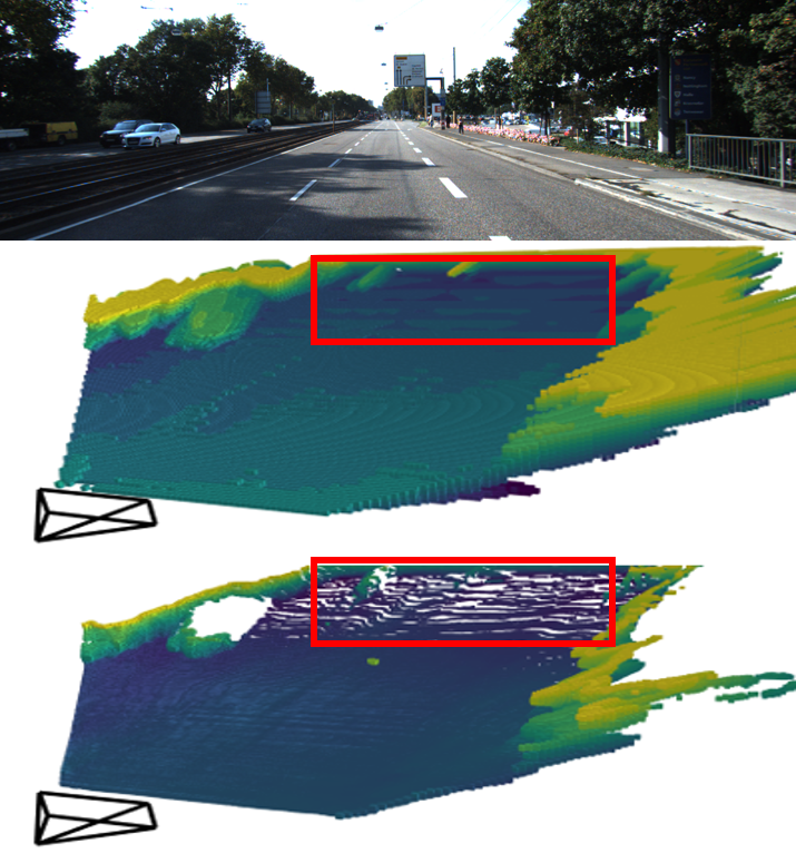
Figure 6: Visualization for depth-map-based representation and the proposed NeRF-like representation. From top to bottom: input image, NeRF-like representation, depth-map-based representation. Our method generates denser features for distant objects.

In Figure 6, we replace the proposed representation with depth-transformed one used in previous works [12, 47] and visualize them for comparison. For depth-transformed category, we first predict the depth map from the input RGB image and apply the same transformation as CaDDN [47] to get its 3D representation. We visualize such representation by back-projecting the estimated depth map to the 3D space. For the NeRF-like representation, we directly visualize the predicted 3D volume density. Our method produces dense and continuous geometry in the distance (as indicated by the red box area). Due to space constraints, we provide additional quantitative and qualitative results in the Supplementary materials. Occupancy results are best viewed as videos, so we urge readers to view our supplementary video.

6 Conclusion

In this paper, we explore how to optimize the intermediate 3D feature representations implicitly for monocular 3D object detection (M3D) without explicit binary occupancy annotations. We build a bridge between Neural Radiance Fields (NeRF) and 3D object detection, and propose a novel monocular 3D object detection framework, i.e. MonoNeRD, which produces continuous NeRF-like Representations for M3D. MonoNeRD treats intermediate 3D representations as SDF-based neural radiance fields and optimizes them using volume rendering techniques. Extensive experiments show that our method sets a new baseline for monocular 3D detection and has the potential to be extended to other 3D perception tasks.

Limitations and future work. The performance of our method is highly dependent on the modeling approaches. We are currently limited by the working with bounds modeling (see Section 3.3), which could fail to predict 3D occupancy when its 2D projected pixel represents sky or other things not within the specified bounds. We believe this is an interesting direction for future research.

References

- [1] Junaid Ahmed Ansari, Sarthak Sharma, Anshuman Majumdar, J Krishna Murthy, and K Madhava Krishna. The earth ain’t flat: Monocular reconstruction of vehicles on steep and graded roads from a moving camera. In 2018 IEEE/RSJ International Conference on Intelligent Robots and Systems (IROS), pages 8404–8410. IEEE, 2018.
- [2] Ivan Barabanau, Alexey Artemov, Evgeny Burnaev, and Vyacheslav Murashkin. Monocular 3d object detection via geometric reasoning on keypoints. arXiv preprint arXiv:1905.05618, 2019.
- [3] Jonathan T Barron, Ben Mildenhall, Matthew Tancik, Peter Hedman, Ricardo Martin-Brualla, and Pratul P Srinivasan. Mip-nerf: A multiscale representation for anti-aliasing neural radiance fields. In Proceedings of the IEEE/CVF International Conference on Computer Vision, pages 5855–5864, 2021.
- [4] Anh-Quan Cao and Raoul de Charette. Scenerf: Self-supervised monocular 3d scene reconstruction with radiance fields. In ICCV, 2023.
- [5] Florian Chabot, Mohamed Chaouch, Jaonary Rabarisoa, Céline Teuliere, and Thierry Chateau. Deep manta: A coarse-to-fine many-task network for joint 2d and 3d vehicle analysis from monocular image. In Proceedings of the IEEE conference on computer vision and pattern recognition, pages 2040–2049, 2017.
- [6] Rohan Chabra, Jan E Lenssen, Eddy Ilg, Tanner Schmidt, Julian Straub, Steven Lovegrove, and Richard Newcombe. Deep local shapes: Learning local sdf priors for detailed 3d reconstruction. In European Conference on Computer Vision, pages 608–625. Springer, 2020.
- [7] Anpei Chen, Zexiang Xu, Andreas Geiger, Jingyi Yu, and Hao Su. Tensorf: Tensorial radiance fields. arXiv preprint arXiv:2203.09517, 2022.
- [8] Anpei Chen, Zexiang Xu, Fuqiang Zhao, Xiaoshuai Zhang, Fanbo Xiang, Jingyi Yu, and Hao Su. Mvsnerf: Fast generalizable radiance field reconstruction from multi-view stereo. In Proceedings of the IEEE/CVF International Conference on Computer Vision, pages 14124–14133, 2021.
- [9] Hansheng Chen, Yuyao Huang, Wei Tian, Zhong Gao, and Lu Xiong. Monorun: Monocular 3d object detection by reconstruction and uncertainty propagation. In Proceedings of the IEEE/CVF Conference on Computer Vision and Pattern Recognition, pages 10379–10388, 2021.
- [10] Xiaozhi Chen, Kaustav Kundu, Ziyu Zhang, Huimin Ma, Sanja Fidler, and Raquel Urtasun. Monocular 3d object detection for autonomous driving. In Proceedings of the IEEE conference on computer vision and pattern recognition, pages 2147–2156, 2016.
- [11] Xiaozhi Chen, Kaustav Kundu, Yukun Zhu, Huimin Ma, Sanja Fidler, and Raquel Urtasun. 3d object proposals using stereo imagery for accurate object class detection. IEEE transactions on pattern analysis and machine intelligence, 40(5):1259–1272, 2017.
- [12] Yi-Nan Chen, Hang Dai, and Yong Ding. Pseudo-stereo for monocular 3d object detection in autonomous driving. In Proceedings of the IEEE/CVF Conference on Computer Vision and Pattern Recognition, pages 887–897, 2022.
- [13] Zhiqin Chen and Hao Zhang. Learning implicit fields for generative shape modeling. In Proceedings of the IEEE/CVF Conference on Computer Vision and Pattern Recognition, pages 5939–5948, 2019.
- [14] Julian Chibane, Aayush Bansal, Verica Lazova, and Gerard Pons-Moll. Stereo radiance fields (srf): Learning view synthesis for sparse views of novel scenes. In Proceedings of the IEEE/CVF Conference on Computer Vision and Pattern Recognition, pages 7911–7920, 2021.
- [15] Julian Chibane, Gerard Pons-Moll, et al. Neural unsigned distance fields for implicit function learning. Advances in Neural Information Processing Systems, 33:21638–21652, 2020.
- [16] Mingyu Ding, Yuqi Huo, Hongwei Yi, Zhe Wang, Jianping Shi, Zhiwu Lu, and Ping Luo. Learning depth-guided convolutions for monocular 3d object detection. In Proceedings of the IEEE/CVF Conference on Computer Vision and Pattern Recognition Workshops, pages 1000–1001, 2020.
- [17] Andreas Geiger, Philip Lenz, and Raquel Urtasun. Are we ready for autonomous driving? the kitti vision benchmark suite. In 2012 IEEE conference on computer vision and pattern recognition, pages 3354–3361. IEEE, 2012.
- [18] Kyle Genova, Forrester Cole, Daniel Vlasic, Aaron Sarna, William T Freeman, and Thomas Funkhouser. Learning shape templates with structured implicit functions. In Proceedings of the IEEE/CVF International Conference on Computer Vision, pages 7154–7164, 2019.
- [19] Xiaoyang Guo, Shaoshuai Shi, Xiaogang Wang, and Hongsheng Li. Liga-stereo: Learning lidar geometry aware representations for stereo-based 3d detector. In Proceedings of the IEEE/CVF International Conference on Computer Vision, pages 3153–3163, 2021.
- [20] Yuxuan Han, Ruicheng Wang, and Jiaolong Yang. Single-view view synthesis in the wild with learned adaptive multiplane images. arXiv preprint arXiv:2205.11733, 2022.
- [21] Tong He and Stefano Soatto. Mono3d++: Monocular 3d vehicle detection with two-scale 3d hypotheses and task priors. In Proceedings of the AAAI Conference on Artificial Intelligence, pages 8409–8416, 2019.
- [22] Peter Hedman, Pratul P Srinivasan, Ben Mildenhall, Jonathan T Barron, and Paul Debevec. Baking neural radiance fields for real-time view synthesis. In Proceedings of the IEEE/CVF International Conference on Computer Vision, pages 5875–5884, 2021.
- [23] Chiyu Jiang, Avneesh Sud, Ameesh Makadia, Jingwei Huang, Matthias Nießner, Thomas Funkhouser, et al. Local implicit grid representations for 3d scenes. In Proceedings of the IEEE/CVF Conference on Computer Vision and Pattern Recognition, pages 6001–6010, 2020.
- [24] Abhinav Kumar, Garrick Brazil, Enrique Corona, Armin Parchami, and Xiaoming Liu. DEVIANT: Depth EquiVarIAnt NeTwork for Monocular D Object Detection. In ECCV, 2022.
- [25] Jiaxin Li, Zijian Feng, Qi She, Henghui Ding, Changhu Wang, and Gim Hee Lee. Mine: Towards continuous depth mpi with nerf for novel view synthesis. In Proceedings of the IEEE/CVF International Conference on Computer Vision, pages 12578–12588, 2021.
- [26] Yingyan Li, Yuntao Chen, Jiawei He, and Zhaoxiang Zhang. Densely constrained depth estimator for monocular 3d object detection. In Computer Vision–ECCV 2022: 17th European Conference, Tel Aviv, Israel, October 23–27, 2022, Proceedings, Part IX, pages 718–734. Springer, 2022.
- [27] Qing Lian, Peiliang Li, and Xiaozhi Chen. Monojsg: Joint semantic and geometric cost volume for monocular 3d object detection. In Proceedings of the IEEE/CVF Conference on Computer Vision and Pattern Recognition, pages 1070–1079, 2022.
- [28] Lingjie Liu, Jiatao Gu, Kyaw Zaw Lin, Tat-Seng Chua, and Christian Theobalt. Neural sparse voxel fields. Advances in Neural Information Processing Systems, 33:15651–15663, 2020.
- [29] Yuxuan Liu, Yuan Yixuan, and Ming Liu. Ground-aware monocular 3d object detection for autonomous driving. IEEE Robotics and Automation Letters, 6(2):919–926, 2021.
- [30] Ilya Loshchilov and Frank Hutter. Decoupled weight decay regularization. arXiv preprint arXiv:1711.05101, 2017.
- [31] Yan Lu, Xinzhu Ma, Lei Yang, Tianzhu Zhang, Yating Liu, Qi Chu, Junjie Yan, and Wanli Ouyang. Geometry uncertainty projection network for monocular 3d object detection. In Proceedings of the IEEE/CVF International Conference on Computer Vision, pages 3111–3121, 2021.
- [32] Xinzhu Ma, Shinan Liu, Zhiyi Xia, Hongwen Zhang, Xingyu Zeng, and Wanli Ouyang. Rethinking pseudo-lidar representation. In European Conference on Computer Vision, pages 311–327. Springer, 2020.
- [33] Xinzhu Ma, Zhihui Wang, Haojie Li, Pengbo Zhang, Wanli Ouyang, and Xin Fan. Accurate monocular 3d object detection via color-embedded 3d reconstruction for autonomous driving. In Proceedings of the IEEE/CVF International Conference on Computer Vision, pages 6851–6860, 2019.
- [34] Fabian Manhardt, Wadim Kehl, and Adrien Gaidon. Roi-10d: Monocular lifting of 2d detection to 6d pose and metric shape. In Proceedings of the IEEE/CVF Conference on Computer Vision and Pattern Recognition, pages 2069–2078, 2019.
- [35] Nelson Max. Optical models for direct volume rendering. IEEE Transactions on Visualization and Computer Graphics, 1(2):99–108, 1995.
- [36] Lars Mescheder, Michael Oechsle, Michael Niemeyer, Sebastian Nowozin, and Andreas Geiger. Occupancy networks: Learning 3d reconstruction in function space. In Proceedings of the IEEE/CVF conference on computer vision and pattern recognition, pages 4460–4470, 2019.
- [37] Mateusz Michalkiewicz, Jhony K Pontes, Dominic Jack, Mahsa Baktashmotlagh, and Anders Eriksson. Implicit surface representations as layers in neural networks. In Proceedings of the IEEE/CVF International Conference on Computer Vision, pages 4743–4752, 2019.
- [38] Ben Mildenhall, Pratul P Srinivasan, Matthew Tancik, Jonathan T Barron, Ravi Ramamoorthi, and Ren Ng. Nerf: Representing scenes as neural radiance fields for view synthesis. Communications of the ACM, 65(1):99–106, 2021.
- [39] Michael Niemeyer, Jonathan T Barron, Ben Mildenhall, Mehdi SM Sajjadi, Andreas Geiger, and Noha Radwan. Regnerf: Regularizing neural radiance fields for view synthesis from sparse inputs. In Proceedings of the IEEE/CVF Conference on Computer Vision and Pattern Recognition, pages 5480–5490, 2022.
- [40] Dennis Park, Rares Ambrus, Vitor Guizilini, Jie Li, and Adrien Gaidon. Is pseudo-lidar needed for monocular 3d object detection? In Proceedings of the IEEE/CVF International Conference on Computer Vision, pages 3142–3152, 2021.
- [41] Jeong Joon Park, Peter Florence, Julian Straub, Richard Newcombe, and Steven Lovegrove. Deepsdf: Learning continuous signed distance functions for shape representation. In Proceedings of the IEEE/CVF conference on computer vision and pattern recognition, pages 165–174, 2019.
- [42] Adam Paszke, Sam Gross, Francisco Massa, Adam Lerer, James Bradbury, Gregory Chanan, Trevor Killeen, Zeming Lin, Natalia Gimelshein, Luca Antiga, et al. Pytorch: An imperative style, high-performance deep learning library. Advances in neural information processing systems, 32, 2019.
- [43] Liang Peng, Xiaopei Wu, Zheng Yang, Haifeng Liu, and Deng Cai. Did-m3d: Decoupling instance depth for monocular 3d object detection. In European Conference on Computer Vision, pages 71–88. Springer, 2022.
- [44] Songyou Peng, Michael Niemeyer, Lars Mescheder, Marc Pollefeys, and Andreas Geiger. Convolutional occupancy networks. In European Conference on Computer Vision, pages 523–540. Springer, 2020.
- [45] Jonah Philion and Sanja Fidler. Lift, splat, shoot: Encoding images from arbitrary camera rigs by implicitly unprojecting to 3d. In European Conference on Computer Vision, pages 194–210. Springer, 2020.
- [46] Zengyi Qin, Jinglu Wang, and Yan Lu. Monogrnet: A geometric reasoning network for monocular 3d object localization. In Proceedings of the AAAI Conference on Artificial Intelligence, pages 8851–8858, 2019.
- [47] Cody Reading, Ali Harakeh, Julia Chae, and Steven L Waslander. Categorical depth distribution network for monocular 3d object detection. In Proceedings of the IEEE/CVF Conference on Computer Vision and Pattern Recognition, pages 8555–8564, 2021.
- [48] Thomas Roddick, Alex Kendall, and Roberto Cipolla. Orthographic feature transform for monocular 3d object detection. arXiv preprint arXiv:1811.08188, 2018.
- [49] Shunsuke Saito, Zeng Huang, Ryota Natsume, Shigeo Morishima, Angjoo Kanazawa, and Hao Li. Pifu: Pixel-aligned implicit function for high-resolution clothed human digitization. In Proceedings of the IEEE/CVF International Conference on Computer Vision, pages 2304–2314, 2019.
- [50] Xuepeng Shi, Qi Ye, Xiaozhi Chen, Chuangrong Chen, Zhixiang Chen, and Tae-Kyun Kim. Geometry-based distance decomposition for monocular 3d object detection. In Proceedings of the IEEE/CVF International Conference on Computer Vision, pages 15172–15181, 2021.
- [51] Siddharth Srivastava, Frederic Jurie, and Gaurav Sharma. Learning 2d to 3d lifting for object detection in 3d for autonomous vehicles. In 2019 IEEE/RSJ International Conference on Intelligent Robots and Systems (IROS), pages 4504–4511. IEEE, 2019.
- [52] Pei Sun, Henrik Kretzschmar, Xerxes Dotiwalla, Aurelien Chouard, Vijaysai Patnaik, Paul Tsui, James Guo, Yin Zhou, Yuning Chai, Benjamin Caine, et al. Scalability in perception for autonomous driving: Waymo open dataset. In Proceedings of the IEEE/CVF conference on computer vision and pattern recognition, pages 2446–2454, 2020.
- [53] Li Wang, Liang Du, Xiaoqing Ye, Yanwei Fu, Guodong Guo, Xiangyang Xue, Jianfeng Feng, and Li Zhang. Depth-conditioned dynamic message propagation for monocular 3d object detection. In Proceedings of the IEEE/CVF Conference on Computer Vision and Pattern Recognition, pages 454–463, 2021.
- [54] Li Wang, Li Zhang, Yi Zhu, Zhi Zhang, Tong He, Mu Li, and Xiangyang Xue. Progressive coordinate transforms for monocular 3d object detection. Advances in Neural Information Processing Systems, 34:13364–13377, 2021.
- [55] Yan Wang, Wei-Lun Chao, Divyansh Garg, Bharath Hariharan, Mark Campbell, and Kilian Q Weinberger. Pseudo-lidar from visual depth estimation: Bridging the gap in 3d object detection for autonomous driving. In Proceedings of the IEEE/CVF Conference on Computer Vision and Pattern Recognition, pages 8445–8453, 2019.
- [56] Zhou Wang, Alan C Bovik, Hamid R Sheikh, and Eero P Simoncelli. Image quality assessment: from error visibility to structural similarity. IEEE transactions on image processing, 13(4):600–612, 2004.
- [57] Felix Wimbauer, Nan Yang, Christian Rupprecht, and Daniel Cremers. Behind the scenes: Density fields for single view reconstruction. arXiv preprint arXiv:2301.07668, 2023.
- [58] Bin Xu and Zhenzhong Chen. Multi-level fusion based 3d object detection from monocular images. In Proceedings of the IEEE conference on computer vision and pattern recognition, pages 2345–2353, 2018.
- [59] Lior Yariv, Jiatao Gu, Yoni Kasten, and Yaron Lipman. Volume rendering of neural implicit surfaces. Advances in Neural Information Processing Systems, 34:4805–4815, 2021.
- [60] Yurong You, Yan Wang, Wei-Lun Chao, Divyansh Garg, Geoff Pleiss, Bharath Hariharan, Mark Campbell, and Kilian Q Weinberger. Pseudo-lidar++: Accurate depth for 3d object detection in autonomous driving. arXiv preprint arXiv:1906.06310, 2019.
- [61] Alex Yu, Ruilong Li, Matthew Tancik, Hao Li, Ren Ng, and Angjoo Kanazawa. Plenoctrees for real-time rendering of neural radiance fields. In Proceedings of the IEEE/CVF International Conference on Computer Vision, pages 5752–5761, 2021.
- [62] Alex Yu, Vickie Ye, Matthew Tancik, and Angjoo Kanazawa. pixelnerf: Neural radiance fields from one or few images. In Proceedings of the IEEE/CVF Conference on Computer Vision and Pattern Recognition, pages 4578–4587, 2021.
- [63] Zehao Yu, Songyou Peng, Michael Niemeyer, Torsten Sattler, and Andreas Geiger. Monosdf: Exploring monocular geometric cues for neural implicit surface reconstruction. arXiv preprint arXiv:2206.00665, 2022.
- [64] Kai Zhang, Gernot Riegler, Noah Snavely, and Vladlen Koltun. Nerf++: Analyzing and improving neural radiance fields. arXiv preprint arXiv:2010.07492, 2020.
- [65] Yunpeng Zhang, Jiwen Lu, and Jie Zhou. Objects are different: Flexible monocular 3d object detection. In Proceedings of the IEEE/CVF Conference on Computer Vision and Pattern Recognition, pages 3289–3298, 2021.
- [66] Yunsong Zhou, Yuan He, Hongzi Zhu, Cheng Wang, Hongyang Li, and Qinhong Jiang. Monocular 3d object detection: An extrinsic parameter free approach. In Proceedings of the IEEE/CVF Conference on Computer Vision and Pattern Recognition, pages 7556–7566, 2021.