DReg-NeRF: Deep Registration for Neural Radiance Fields

Abstract

Although Neural Radiance Fields (NeRF) is popular in the computer vision community recently, registering multiple NeRFs has yet to gain much attention. Unlike the existing work, NeRF2NeRF [14], which is based on traditional optimization methods and needs human annotated keypoints, we propose DReg-NeRF to solve the NeRF registration problem on object-centric scenes without human intervention. After training NeRF models, our DReg-NeRF first extracts features from the occupancy grid in NeRF. Subsequently, our DReg-NeRF utilizes a transformer architecture with self-attention and cross-attention layers to learn the relations between pairwise NeRF blocks. In contrast to state-of-the-art (SOTA) point cloud registration methods, the decoupled correspondences are supervised by surface fields without any ground truth overlapping labels. We construct a novel view synthesis dataset with 1,700+ 3D objects obtained from Objaverse to train our network. When evaluated on the test set, our proposed method beats the SOTA point cloud registration methods by a large margin with a mean $\text{RPE}=9.67^{\circ}$ and a mean $\text{RTE}=0.038$. Our code is available at https://github.com/AIBluefisher/DReg-NeRF.

Figure 1: Our method registers multiple NeRF blocks. (a) One of the collected objects from the Objaverse [10] dataset. We render the images from a predefined camera trajectory to construct our training data. (b) NeRF models are trained in different coordinate frames. (c) Our method aligns NeRF blocks into the same coordinate frame without accessing raw image data.

1 Introduction

Scene reconstruction has many applications in the real world, for example, in augmented reality, ancient culture preservation, 3D content generation, etc. Recently, rapid progress has been made in increasing the reconstruction quality using neural radiance fields (NeRF) [27]. While previous works mostly focused on synthesizing images at the object level or unbounded scenes within a small area, Block-NeRF [35] extends NeRF to city-scale scenes by splitting data into multiple intersected blocks. Specifically, Block-NeRF trains multiple NeRF models in the same coordinate frame with the ground-truth camera poses provided by fusing multiple high-precision sensors. However, images can be collected without absolute pose information in some cases, e.g., when images are captured with digital cameras or in GPS-denied areas. In such cases, Block-NeRF cannot work since NeRF models are trained on different coordinate frames. Consequently, NeRF registration [14] is necessary for synthesizing consistent novel views from multiple NeRFs trained in different coordinate frames.

Point cloud registration is a classic problem in 3D computer vision, which aims at computing the relative transformation from the source point cloud to the target point cloud. However, NeRF registration is under-explored since existing works focus mostly on point cloud registration. Unlike point clouds that are simple explicit representation, NeRF encodes scenes implicitly, which makes registering multiple NeRFs more challenging. NeRF2NeRF [14] is the first work that tried to solve registering NeRFs by a traditional optimization-based approach. However, it requires human-annotated keypoints for initialization, which limits its application in the real world where human annotations can be impractical. In view of the above-mentioned challenges, we focus on the study of the NeRF registration problem by answering the following two questions: 1) Can we register two or multiple NeRFs together where only pre-trained models are accessible? 2) How to register NeRFs without any human annotations and initializations?

We further use the following settings in our endeavor to answer the two challenging questions on NeRF registration: 1) Images are collected into different blocks and no images are associated with known absolute position information. 2) Multiple NeRF blocks are trained individually where ground truth camera poses in each block are in their local coordinate frames. 3) Only the trained NeRF models are accessible, and all training images are removed and therefore not available due to plausible privacy-preserving issues or disk limitations. We emphasize that NeRF registration is a challenging task, and we focus more on the object-centric scenes in this paper. See Fig. 1 for the illustration of our task setting and dataset construction.

To solve the NeRF registration problem, we first utilize an occupancy grid along with each NeRF model to extract a voxel grid. The voxel grid is then fed into a 3D Feature Pyramid Network (FPN) [22] to extract features. The resulting voxel feature grids are further processed by a transformer module. In the transformer network, we first adopt a self-attention layer to enhance the intra-feature representations within each voxel feature grid. We further utilize a cross-attention layer to learn the inter-feature relations between the source feature grid and the target feature grid. Finally, we use an attention head to decode the source features and target features into correspondences and confidence scores. Unlike SOTA point clouds registration methods [16, 43], we utilize NeRF as geometric supervision and thus do not rely on pre-computed overlapping scores to mask correspondences outside the overlapping areas.

The main contributions of our work are:

• A dataset for registering multiple NeRF blocks, which is created by rendering $1,700+$ 3D objects that are downloaded from the Objaverse dataset.

• A novel network for registering NeRF blocks which do not rely on any human annotation and initializations.

• Exhaustive experiments to show the accuracy and generalization ability of our method.

To the best of our knowledge, this is the first work on registering NeRFs without a) any initializations from keypoints or other registration methods and b) precomputed ground-truth overlapping labels.

2 Related Work

Neural Radiance Fields.

The differentiable volume rendering technique makes neural networks suitable for encoding scene representations. Vanilla NeRF [27] needs to take days to train each scene. NSVF [25] encodes scenes explicitly in a sparse voxel grid with online pruning, which improves the training and rendering efficiency by a large margin. PlenOctree [44] adopted the voxel representation, and further decouple the radiance field from view directions by spherical harmonics. To further accelerate the network training, PlenOctree finetunes the voxel grid by directly optimizing the stored features without accessing any neural networks. Plenoxels [13] optimizes voxel features without any neural network for initialization. The training speed is accelerated with a specifically designed CUDA optimizer. InstantNGP [28] encodes voxel features implicitly into a multi-resolution hash grid. TensoRF [4] decomposes 3D voxel into low-rank vector-matrix multiplications. Its training speed is comparable to InstantNGP even without a CUDA implementation.

Block-NeRF [35] partition the collected images into different street blocks, each block is trained individually along with jointly optimizing camera poses [21, 5]. The final images can be synthesized by fusing from multiple nearby NeRF blocks. Mega-NeRF [38] also adopted the same divide-and-conquer strategy as BlockNeRF, but focus more on aerial images and exploiting the sparse network structures. To train their network, Block-NeRF obtained camera poses by fusing data from different sensors, while Mega-NeRF used Structure from Motion (SfM) [24, 9, 7, 8] tools to recover camera poses. Both of them assume camera poses are in the same coordinate frames.

Point Cloud Registration.

The Iterative Closest Point (ICP) [2, 6] algorithm has been widely applied to the industry community and research community for years. Given a rough initialization, ICP tries to align the source point cloud to the target point cloud. The global point cloud registration methods can align point clouds without initialization by extracting geometric features such as the Fast Point Feature Histograms (FPFH) [31]. To solve the long-time issue of the global registration method in evaluating candidate models within RANSAC [12], Zhou and Park [46] proposed a fast approach that does not need to evaluate the candidate models at each iteration. Deep point cloud registration methods also gained much attention nowadays. Deep Closest Point  [42] is a learned variant of the classical ICP. Inspired by SuperGlue [33], which is a deep learning method for matching 2D image correspondences, Predator [16] and REGTR [43] adopted the self-attention and cross-attention mechanisms from SuperGlue to learn the correlation for pairwise low-overlapping point clouds. The ground-truth overlapping scores are computed from dense point clouds and used to mask out the correspondences outside the overlapping regions. We also follow the previous attention mechanisms, but do not rely on the pre-computed overlapping labels.

NeRF Registration.

NeRF2NeRF [14] is the first work that tries to register multiple NeRFs. The initial transformation is estimated from human-annotated keypoints, and then refined by the surface fields from NeRF. To reduce the number of useless samples, NeRF2NeRF adopts Metropolis-Hasting sampling to maintain an active set. The whole framework is based on traditional optimization methods and needs human interaction. ZeroNeRF [29] claims it can register NeRF without overlap. However, it still requires a global registration method for initialization. Unlike the previous works, which rely heavily on traditional optimization methods, we try to register multiple NeRF blocks by learning methods without human interaction.

3 Our Method

Figure 2: Network architecture of our method. The pipeline of our method is: 1) We first extract the pairwise voxel grid $\mathbf{G}\in\mathbb{R}^{x_{\text{ref}}\times y_{\text{res}}\times z_{\text{res}}\times C}$ and a binary mask $\mathbf{M}\in\mathbb{R}^{x_{\text{ref}}\times y_{\text{res}}\times z_{\text{res}}\times 1}$ from the source NeRF and the target NeRF. 2) The voxel grid $\mathbf{G}$ and a binary mask $\mathbf{M}$ are fed into the 3D feature pyramid network to extract voxel features. 3) The extracted voxel grid features are downsampled to a 2-dimensional tensor $\mathcal{F}\in\mathbb{R}^{N\times C^{{}^{\prime}}}$ by their spherical neighborhood. 4) The resulting source features $\mathcal{F}_{\text{source}}$ and target features $\mathcal{F}_{\text{target}}$ are strengthened by a transformer, where a self-attention layer is used to enhance the intra-contextual relations, and a cross-attention layer is used to learn the inter-contextual relations. 5) Finally, we use a single-head attention layer to decode the features into correspondences and their corresponding confidence scores.

Fig. 2 shows an illustration of our framework. Our network takes a source NeRF model and a target NeRF model as input, and outputs correspondences in the source NeRF and target NeRF. We first train multiple NeRF blocks in different coordinate frames. For each NeRF model, we associate it with an occupancy voxel grid, where each voxel indicates whether it is occupied or not. After training, we extract a 3D voxel grid for each NeRF model and then feed it into a 3D CNN backbone to extract features. Subsequently, we use a transformer with self-attention and cross-attention layers to learn the relations between the pairwise feature grids. We then adopt a decoder to decode the resulting features $\mathcal{F}_{\text{source}},\mathcal{F}_{\text{target}}$ into correspondences $\{\mathbf{X}_{\text{source}},\mathbf{X}_{\text{target}}\}$ and the corresponding confidence scores $\{\mathbf{S}_{\text{source}},\mathbf{S}_{\text{target}}\}$. Finally, the relative transformation can be solved by the weighted Kabsch-Umeyama algorithm [39] from the correspondences.

3.1 Background

Neural Radiance Fields.

Neural Radiance Fields (NeRF) aims at rendering photo-realistic images from a new view point. For a 3D point $\mathbf{X}$, the density field $\sigma_{t}$ of $\mathbf{X}$ is defined as the differential probability of a ray $\mathbf{r}=(\mathbf{o},\mathbf{d})$ hitting a particle, where $\mathbf{o}$ is the camera center, $\mathbf{d}$ is the view direction. The transmittance $\mathcal{T}(t)$ denotes the probability of ray without hitting any particles when traveling a distance $t$, and the discrete form of $\mathcal{T}(t)$ is:

$$\mathcal{T}_{n}=\mathcal{T}(0\rightarrow t_{n})=\exp\big{(}\sum_{k=1}^{n-1}-\sigma_{k}\delta_{k}\big{)}.$$ (1)

Given a set of points $\{\mathbf{X}_{n}=\mathbf{o}+t_{n}\mathbf{d}\ |\ n\in[0,K]\}$, NeRF predicts the view-independent volume density $\sigma_{n}$ and view-dependent radiance field by:

$$\sigma_{n},\mathbf{e}_{n}=\mathbf{F}(\mathbf{X};\mathbf{\Theta}),$$

$$\mathbf{c}_{n}=\mathbf{F}(\mathbf{r},\mathbf{e};\mathbf{\Theta}),$$ (2)

where $\mathbf{e}_{n}$ is an embedding vector and $\Theta$ denotes the network parameters. The final color of an image pixel can be rendered by:

$$\mathbf{C}(t_{N+1})=\sum_{n=1}^{N}\mathcal{T}_{n}\cdot\big{(}1-\exp(-\sigma_{n}\delta_{n})\big{)}\cdot\mathbf{c}_{n}.$$ (3)

We recommend interested readers to refer to [27, 34] for the detailed derivation.

3.2 Querying Radiance Fields from NeRF

To extract features for the latter learning modules, we first construct a 3D volume from NeRF. Specifically, we assume each NeRF is trained within a bounding box with a 3D voxel grid of resolution $[x_{\text{ref}},y_{\text{res}},z_{\text{res}}]$. We then obtain the point locations $\{\mathbf{X}\}$ of voxel centers. We also obtain a binary occupancy mask $\mathbf{M}_{\text{occ}}$ from the occupancy grid, where voxels that are not occupied denote empty space and thus are ignored. The occupancy grid is the acceleration structure used in InstantNGP [28] to skip empty space in NeRF training. Each grid has a resolution of $128^{3}$ that is centered around $(0,0,0)$ and stores occupancy as a single bit. During ray marching, a sample point is skipped if the bit of a grid cell is low. We can query the density fields $\{\sigma\}$ and radiance fields $\{\mathbf{c}\}$ using Eq. (3.1) with the coordinates $\{\mathbf{X}\}$. Since density fields can be noisy, we further obtain a density mask $\mathbf{M}_{\text{df}}=\sigma>\sigma_{t}$ by setting a threshold $\sigma_{t}$ (we use $\sigma_{t}=0.7)$. We then obtain our mask as $\mathbf{M}=\mathbf{M}_{\text{occ}}\cap\mathbf{M}_{\text{df}}$.

One issue with radiance fields is that they are view-dependent. However, the training views are different for each NeRF block. Suppose the NeRF is trained by $N$ views with camera poses $\mathbf{P}=[\mathbf{R}\mid\mathbf{t}]$ which project points from camera frame to world frame. To obtain the radiance fields, we form $N$ viewing rays $\mathbf{r}=\mathbf{o}+t\mathbf{d}$, where $\mathbf{d}=\frac{\mathbf{X}-\mathbf{t}}{\|\mathbf{X}-\mathbf{t}\|}$ for each query point and average the queried radiance fields over all rays. The final color $\mathbf{C}$ can be obtained by volume rendering of Eq. (3). Furthermore, we compute the alpha compositing value by $\alpha=1-\exp(-\sigma\delta)$, where $\delta$ is a chosen small value. We associate each point in the voxel grid with $[\mathbf{X},\mathbf{C},\alpha]$ and feed the voxel grid $\mathbf{G}\in\mathbb{R}^{x_{\text{ref}}\times y_{\text{res}}\times z_{\text{res}}\times C}$ and a mask $\mathbf{M}\in\mathbb{R}^{x_{\text{ref}}\times y_{\text{res}}\times z_{\text{res}}\times 1}$ into a 3D CNN to extract backbone features, where $C=7$ with $3$ channels from the point coordinate, three from the color channels, and one from the scalar $\alpha$.

3.3 Feature Extraction

Given the voxel grid, we adopt the feature pyramid network [22] to extract features. We use ResNet [15] as the feature backbone, where all the 2D modules are replaced by their corresponding 3D parts. The feature pyramid network enables the learning of high-level semantic features at a multi-scale and thus is suitable to extract the voxel grid features in our task settings. We note the difference from the original feature pyramid network which utilizes different scale features for object detection, we adopt only the features output from the last layer. Since the dimension of the feature grid from the last layer can be different from the original voxel grid, we rescale it to the size of the original voxel grid $\mathbf{G}$ and resulted in a voxel feature grid $\mathbf{G}_{f}\in\mathbb{R}^{x_{\text{ref}}\times y_{\text{res}}\times z_{\text{res}}\times C^{{}^{\prime}}}$.

We cannot use $\mathbf{G}_{f}$ as the input to our transformer since the voxel feature grid can contain too many points to enable the transformer to run on a single GPU. To solve this issue, we iteratively downsample $\mathbf{G}_{f}$ by the spherical neighborhood [36] as done in KPConv [37] to obtain the downsampled voxel points $\hat{\mathbf{X}}$. The downsample iteration is terminated when the total number of occupied voxels in the current sampled voxel feature grid is less than $1.5$K. Lastly, we reshape the occupied voxel features into a tensor $\mathbf{\mathcal{F}}\in\mathbb{R}^{N\times C^{{}^{\prime}}}$. The weights of the feature extraction network are shared across the source and the target NeRFs. We denote the downsampled voxel points and extracted features of the source and target NeRFs as: $[\hat{\mathbf{X}}_{\text{source}},\mathcal{F}_{\text{source}}]$ and $[\hat{\mathbf{X}}_{\text{target}},\mathcal{F}_{\text{target}}]$, respectively.

3.4 Transformer

We then feed the resulting feature $\mathcal{F}_{\text{source}}$ and $\mathcal{F}_{\text{target}}$ into a $L$-layer transformer with self-attention and cross-attention layers. We follow the same intuition of Predator [16] and REGTR [43], where a self-attention layer is applied to both the source feature $\mathcal{F}_{\text{source}}$ and the target feature $\mathcal{F}_{\text{target}}$ to enhance the intra-contextual relations, and a cross-attention layer is applied to both $\mathcal{F}_{\text{source}}$ and $\mathcal{F}_{\text{target}}$ to learn the inter-contextual relations. We follow the classical transformer architecture [41, 20, 43] with input to be voxel features.

Multi-Head Attention.

The multi-head attention operation in each layer is defined as:

$$\text{MH}(\mathbf{Q},\mathbf{K},\mathbf{V})=\text{concat}(\text{head}_{1},\cdots,\text{head}_{h})\mathbf{W}^{O},$$ (4)

where $\text{head}_{i}=\text{Attention}(\mathbf{Q}\mathbf{W}^{Q}_{i},\mathbf{K}\mathbf{W}_{i}^{K},\mathbf{V}\mathbf{W}_{i}^{V})$. The attention function is adopted as the scaled dot-product:

$$\text{Attention}(\mathbf{Q},\mathbf{K},\mathbf{V})=\text{softmax}(\frac{\mathbf{Q}\mathbf{K}^{\top}}{\sqrt{d_{k}}})\mathbf{V}.$$ (5)

In the self-attention layers, $\mathbf{Q}=\mathbf{K}=\mathbf{V}$ represents the same feature tensor in each block. In the cross-attention layers, the keys, and the values are the feature tensors from the other block. The self-attention mechanism enables the network to learn the relationship inside the same feature points, while the cross-attention mechanism enables the communication of the different feature points.

Decoder.

After encoding features by transformer, we further adopt a single-head attention layer to predict the corresponding point locations $\tilde{\mathbf{X}}_{\text{source}}$ and confidence scores $\tilde{\mathbf{S}}_{\text{source}}$ of the source voxel points $\hat{\mathbf{X}}_{\text{source}}$ in the target NeRF’s coordinate frame. Similarly, we also predict the corresponding point locations $\tilde{\mathbf{X}}_{\text{target}}$ and confidence scores $\tilde{\mathbf{S}}_{\text{target}}$ of the target voxel points $\hat{\mathbf{X}}_{\text{target}}$ in the source NeRF’s coordinate frame. Finally, we utilize the predicted correspondences to compute the relative rigid transformation. The confidence scores are used as weights that mask out the irrelevant correspondences and can be interpreted as how likely the predicted points from $\tilde{\mathbf{X}}_{\text{source}}$ and $\tilde{\mathbf{X}}_{\text{target}}$ are correspondences and are visible in the source NeRF and the target NeRF.

3.5 Training Loss

Surface Field Supervision.

To train the network, we encourage the predicted correspondences to have the same features which are invariant in the corresponding NeRF model. The naïve way is to adopt density fields as supervision instead of radiance fields since density fields are invariant to view points. However, density fields can be very noisy. We thus utilize the surface fields [14] as supervision. The surface field is defined as the differential probability of the ray hitting a surface at $\mathbf{X}_{n}$ given by:

$$\mathcal{S}(t)=\mathcal{T}(t)\cdot(1-\exp(-2\sigma\delta)).$$ (6)

Proof:

The differential probability of a ray hitting a surface at point $\mathbf{X}$ is the product of the probability of a ray traveling over $[0,t_{n})$ without hitting any particle before $t_{n}$ times the differential probability of the ray hitting exactly at point $\mathbf{X}(t_{n})$. The surface field can then be written as:

$$S(t)=\int_{t-\delta}^{t+\delta}\mathcal{T}(s)\cdot\sigma(s)\ ds$$ (7)

We derive the exact form of $S(t)$ as follow:

$$S(t) =\int_{t-\delta}^{t+\delta}\mathcal{T}(s)\cdot\sigma(s)\ ds$$

$$=\int_{t-\delta}^{t+\delta}\mathcal{T}(0\rightarrow t-\delta)\cdot\mathcal{T}(t-\delta\rightarrow s)\cdot\sigma(s)\ ds$$

$$=\mathcal{T}(t-\delta)\cdot\int_{t-\delta}^{t+\delta}\mathcal{T}(t-\delta\rightarrow s)\cdot\sigma(s)\ ds$$

$$=\mathcal{T}(t-\delta)\cdot\sigma_{t}\cdot\int_{t-\delta}^{t+\delta}\mathcal{T}(t-\delta\rightarrow s)\ ds$$

$$=\mathcal{T}(t-\delta)\cdot\sigma_{t}\cdot\int_{t-\delta}^{t+\delta}\Big{(}\exp\big{(}-\int_{t-\delta}^{s}\sigma(\mu)\ d\mu\big{)}\Big{)}\ ds$$

$$=\mathcal{T}(t-\delta)\cdot\sigma_{t}\cdot\int_{t-\delta}^{t+\delta}\Big{(}\exp\big{(}-\sigma_{t}(s-t+\sigma)\big{)}\Big{)}\ ds$$

$$=\mathcal{T}(t-\delta)\cdot\sigma_{t}\cdot(-\frac{1}{\sigma_{t}})\cdot\exp\big{(}-\sigma_{t}(s-t+\delta)\big{)}\big{|}_{t-\delta}^{t+\delta}$$

$$=\mathcal{T}(t-\delta)\cdot\big{(}1-\exp(-2\sigma_{t}\cdot\delta)\big{)}.$$ (8)

The second term holds since transmittance is multiplicative (c.f. Eq.(18) of [34]). The 4th term holds since we can assume the density $\sigma_{t}$ is a constant within a small region $[t-\delta,t+\delta]$. To produce the view-independent field, we first form N viewing rays for each point. Subsequently, we take the maximum value of all rays as the density field value instead of averaging the value (as done in Sec. 3.2) for the radiance field. Finally, we obtain the surface field mask $\mathbf{M}_{\text{sf}}$ by checking $S(t)>\eta$ (we use $\eta$ = 0.5). We then update our mask by $\mathbf{M}=\mathbf{M}_{\text{occ}}\ \cap\ \mathbf{M}_{\text{df}}\ \cap\ \mathbf{M}_{\text{sf}}$.

Confidence Loss.

We adopt the cross-entropy loss to supervise the confidence score, with the surface fields $\mathbf{\hat{S}}_{\text{source}}=S(\hat{\mathbf{X}}_{\text{source}}),\mathbf{\hat{S}}_{\text{target}}=S(\hat{\mathbf{X}}_{\text{target}})$ queried from NeRF as the ground truth label:

$$\mathcal{L}_{\text{conf}}=\text{BCE}(\mathbf{\hat{S}}_{\text{source}},\tilde{\mathbf{S}}_{\text{source}})+\text{BCE}(\mathbf{\hat{S}}_{\text{target}},\tilde{\mathbf{S}}_{\text{target}}).$$ (9)

Surface Field Loss.

In addition to the confidence loss, we also encourage the predicted correspondences to have consistent surface field values:

$$\small\mathcal{L}_{\text{sf}}=\frac{1}{N}\|\mathbf{S}([\hat{\mathbf{X}}_{\text{source}},\hat{\mathbf{X}}_{\text{target}}])-\mathbf{S}([\tilde{\mathbf{X}}_{\text{source}},\tilde{\mathbf{X}}_{\text{target}}])\|_{1},$$ (10)

where $N$ is the total number of the concatenated source voxel points and target voxel points.

Correspondence Loss.

We further use a correspondence loss to constrain the predicted locations of correspondences:

$$\mathcal{L}_{\text{corr}}=\sum\rho(\mathbf{S}\|\mathcal{T}^{\star}(\mathbf{x}_{i})-\mathbf{y}_{i}\|;\eta,\gamma),$$ (11)

where $\mathcal{T}^{\star}$ is the ground truth relative transformation between the source NeRF and target NeRF, $\rho(\cdot;\eta,\gamma)$ is the adaptive robust loss function [1] and $\{\eta,\gamma\}$ are respectively a smooth interpolation value and a scale parameter, which are hyperparameters used to control the shape of the robust function. We use $\eta=1.0,\gamma=0.5$ in our experiments.

Moreover, we adopt the feature loss [40, 43] to leverage the geometric properties when computing the correspondences. Our final loss is therefore defined as:

$$\mathcal{L}_{\text{final}}=\mathcal{L}_{\text{conf}}+\lambda_{1}\mathcal{L}_{\text{sf}}+\lambda_{2}\mathcal{L}_{\text{corr}}+\lambda_{3}\mathcal{L}_{\text{feat}},$$ (12)

where $\lambda_{1},\lambda_{2},\lambda_{3}$ are the weights associated with the corresponding loss functions. In our experiments, we use $\lambda_{1}=1.0,\lambda_{2}=0.1,\lambda_{3}=1.0$.

4 Experiments

Figure 3: An overview of our training data. The training images are rendered from 3D objects collected from the Objaverse dataset. We randomly picked $\sim 30$ classes, on which each class contains 40–80 objects.

Datasets.

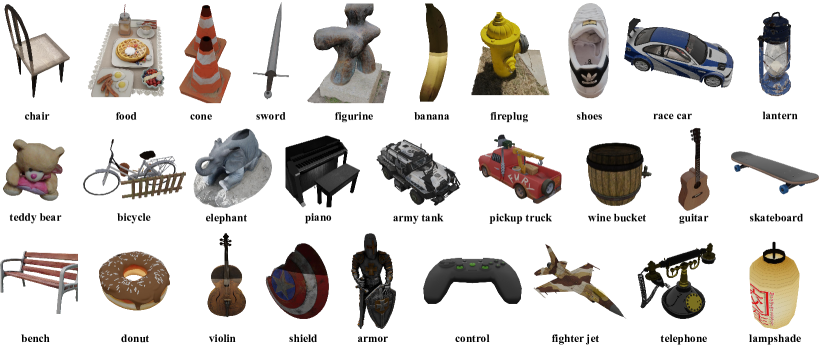
We aim at registering multiple NeRFs. Due to the lack of a suitable dataset for our task, we downloaded the 3D mesh models of $1,700+$ objects from Objaverse [10] to construct our dataset. Objaverse [10] is a massive dataset that contains $800K+$ annotated 3D Objects. It is created for the text-to-3D task. We utilize it to construct our dataset for NeRF registration. Specifically, we randomly selected $30+$ categories and each category contains $40-80$ objects. As Objaverse contains only 3D objects, we render 120 images for each object where the distribution of camera poses can be seen from Fig. 1 (a). We then split the images into 2 blocks by KMeans. We also add a randomly generated transformation to the original camera poses after splitting data into separate blocks, such that NeRF blocks are trained in different coordinate frames. Each NeRF block is trained in $10K$ iterations. See Fig. 3 for an overview of our selected training data. The NeRF models trained on all objects are used to train our NeRF registration neural network, and we randomly select 44 objects that are not seen during training for the test.

Implementations.

We render images for all $1,700+$ objects in a computer with an Intel i7 CPU and an NVIDIA GTX 4090 GPU. We run 8 processes concurrently for downloading the mesh models and the job is finished within a week. We use an occupancy grid with a resolution of $128\times 128\times 128$ associated InstantNGP [28] as our NeRF representation. To train NeRF, we sample 1024 points for each ray. We use Adam [17] as the NeRF optimizer. We set the initial learning rate to $1e-2$ and decay it at step $5K,7.5K,9K$ with a multiplicative factor being $0.33$. Except for storing the NeRF models, we also store the camera poses and intrinsics as metadata. For our NeRF registration network, we use AdamW [26] as the optimizer with weight decay $1e-4$. The learning rate is set to $1e-4$ and halved every $34K$ iteration. The batch size is $1$. Our network is trained for $60$ epochs, which took about 48 hours to finish. For our transformer, we use $L=6$ layers and $h=8$ heads.

		Food 5648	Chair 4b05	Chair 4659	Chair 3f2d	Cone 37b5	Figurine 260d	Figurine 0a5b	Figurine 09f0	Banana 3a07	Banana 2373	Banana 0a07
$\Delta\mathbf{R}$	FGR [46]	178.34	50.50	28.54	81.31	104.52	89.13	26.35	138.00	12.17	6.92	2.86
	REGTR [43]	169.07	150.38	92.80	98.67	62.50	111.80	106.12	176.48	136.02	178.36	173.96
	$\text{Ours}_{\text{df}}$	77.48	160.13	157.21	22.91	108.09	121.32	10.53	95.89	95.43	3.49	6.96
	Ours	6.01	6.53	17.74	18.88	18.79	2.11	7.62	8.25	15.55	10.95	1.36
$\Delta\mathbf{t}$	FGR [46]	17.44	2.27	7.10	8.65	30.49	19.25	10.93	35.22	8.50	1.53	1.36
	REGTR [43]	30.72	15.41	24.97	60.53	84.20	62.07	35.48	42.10	10.75	50.40	13.17
	$\text{Ours}_{\text{df}}$	15.52	7.32	11.72	2.29	21.70	33.61	1.95	21.40	13.14	4.28	0.50
	Ours	1.78	4.13	8.74	5.07	3.06	3.54	10.68	3.18	0.46	1.00	1.22

		Fireplug 06d5	Fireplug 0063	Fireplug 0152	Shoe 18c3	Shoe 1627	Shoe 0bf9	Shoe 022c	Teddy 1b47	Elephant 183a	Elephant 1608	Elephant 1a39
$\Delta\mathbf{R}$	FGR [46]	6.19	20.32	7.50	10.23	178.14	71.55	50.28	8.05	7.65	21.37	30.97
	REGTR [43]	156.92	99.60	4.04	2.55	175.21	97.92	154.91	149.17	177.15	172.28	102.62
	$\text{Ours}_{\text{df}}$	156.17	45.76	12.34	14.69	131.66	158.66	6.84	6.32	6.97	3.92	126.94
	Ours	7.96	17.43	4.86	6.06	12.95	6.48	2.93	11.44	8.00	11.13	13.84
$\Delta\mathbf{t}$	FGR [46]	5.83	0.83	1.17	0.04	4.99	8.82	35.47	1.11	4.51	14.08	11.03
	REGTR [43]	68.71	38.74	2.13	3.53	43.40	61.37	102.00	42.84	52.26	66.15	34.54
	$\text{Ours}_{\text{df}}$	10.54	5.32	2.60	4.66	28.63	24.82	4.40	2.20	4.26	1.40	33.57
	Ours	1.58	5.08	0.96	2.08	12.80	1.81	0.65	1.06	8.97	6.17	7.80

Table 1: Quantitative results (first part) of registration on the Objaverse dataset. $\Delta\mathbf{R}$ denotes the relative rotation errors in degree, $\Delta\mathbf{t}$ denotes the relative translation errors multiplied by 1e2 with unknown scales. FGR [46] denotes the fast global matching method, $\text{Ours}_{\text{df}}$ denotes our method with surface fields replaced by density fields.

		Piano 0e0d	Piano 0a6e	Truck 1431	Guitar 15b4	Guitar 14f8	Guitar 0ceb	Guitar 0aa0	Lantern 0231	Lamp 0230	Bench 0b05	Shield 22a7
$\Delta\mathbf{R}$	FGR [46]	23.09	77.63	7.46	7.80	5.25	13.07	39.94	130.36	17.44	19.51	170.27
	REGTR [43]	30.54	117.90	178.49	5.18	29.47	103.84	5.95	139.32	160.45	122.12	157.38
	$\text{Ours}_{\text{df}}$	160.71	168.79	117.07	11.43	164.87	177.62	7.96	7.76	173.09	179.16	178.00
	Ours	16.30	13.51	16.68	12.60	3.43	1.08	9.53	9.17	16.44	12.98	8.21
$\Delta\mathbf{t}$	FGR [46]	7.43	14.50	5.95	2.86	3.46	1.83	8.42	9.06	0.69	12.52	15.57
	REGTR [43]	44.24	65.99	50.63	15.18	18.41	89.20	9.91	57.25	64.44	31.97	44.29
	$\text{Ours}_{\text{df}}$	22.86	26.18	24.83	10.27	8.50	43.21	4.09	3.35	26.77	28.59	34.71
	Ours	4.80	12.54	0.04	5.72	5.03	3.01	1.20	3.29	1.31	1.68	11.33

		Shield 1973	Shield 14a6	Shield 00ad	Controller 0866	Fighter Jet 16c6	Fighter Jet 089f	Fighter Jet 0000	Telephone 1a8c	Telephone 0354	Lampshade ab66	Skateboard 10c7
$\Delta\mathbf{R}$	FGR [46]	130.83	178.99	7.06	164.01	11.91	40.21	39.86	150.10	19.76	147.50	176.90
	REGTR [43]	138.94	169.78	14.76	102.05	154.74	150.64	178.35	144.47	1.13	148.44	3.88
	$\text{Ours}_{\text{df}}$	178.93	4.92	7.78	179.13	9.75	23.97	178.68	132.49	16.59	5.79	179.97
	Ours	12.94	12.26	2.29	4.03	6.88	10.53	6.46	15.60	9.01	5.67	1.92
$\Delta\mathbf{t}$	FGR [46]	49.44	55.62	0.22	8.97	6.90	11.73	3.44	57.53	18.51	67.08	19.03
	REGTR [43]	72.01	48.56	6.57	65.87	52.97	82.10	28.79	51.09	0.91	54.45	5.14
	$\text{Ours}_{\text{df}}$	59.08	0.66	1.58	23.68	2.64	13.98	19.28	63.76	15.65	4.81	12.20
	Ours	2.79	4.38	1.26	0.99	2.53	7.55	2.09	1.28	3.57	0.81	0.16

Table 2: Quantitative results (second part) of registration on the Objaverse dataset. $\Delta\mathbf{R}$ denotes the relative rotation errors in degree, $\Delta\mathbf{t}$ denotes the relative translation errors multiplied by 1e2 with unknown scales. FGR [46] denotes the fast global matching method, $\text{Ours}_{\text{df}}$ denotes our method with surface fields replaced by density fields.

Figure 4: The qualitative results on Objaverse [10] dataset after NeRF registration. From left to right are respectively the rendered images by the source NeRF model, the rendered images by the target NeRF model, the side view (SV) of the aligned camera poses, the birds-eye-view (BEV) of the aligned camera poses, the concatenated predictions by transforming the source prediction to the target NeRF’s coordinate frame. red and green, respectively, denote the results from source NeRF and target NeRF.

Evaluation.

NeRF2NeRF [14] needs human annotated keypoints for initialization, which are not available on the dataset. Therefore, we do not evaluate NeRF2NeRF on this dataset and use Fast Global Registration (FGR) [46] as the baseline. We also compared it against the state-of-the-art deep point cloud registration method REGTR [43]. For FGR and REGTR, we extract the voxel grid of each NeRF block to a point cloud and use the pairwise point clouds as input to them. For REGTR, we use the model that is pre-trained on the 3DMatch [45] dataset provided by the author. We do not retrain REGTR on the Objaverse dataset since the ground-truth overlapping labels are not available on this dataset. We also evaluated our method $\text{Ours}_{\text{df}}$ with the surface fields replaced by the density fields as a comparison.

Figure 5: Our method failed on unbounded scenes where noisy points are extracted from the occupancy grid.

Results. The quantitative results can be seen from Tab. 1 and Tab. 2. We report the relative rotation errors (RRE) $\Delta\mathbf{R}$ (in degree) and the relative translation errors (RTE) $\Delta\mathbf{t}$ as metrics. Note that the scale of translation is unknown and we multiply $\Delta\mathbf{t}$ by $1e2$. As we can see, FGR [46] failed in most of the scenes. We think it is the low resolution of our voxel grids that makes FGR [46] fail to find the correspondences. REGTR [43] also fails to find the correct transformations in almost all the scenes. It is worse than FGR in both rotations and translations. We also find very poor generalization ability of $\text{Ours}_{\text{df}}$. We conjecture that it is due to the density fields being too noisy and not unique for identifying per-scene geometry. In contrast, “Ours” achieves the best results among almost all the scenes – since the network can be regularized to focus on the scene geometry properties by leveraging the surface fields.

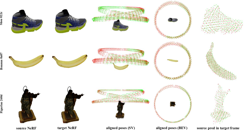
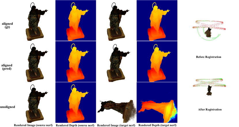
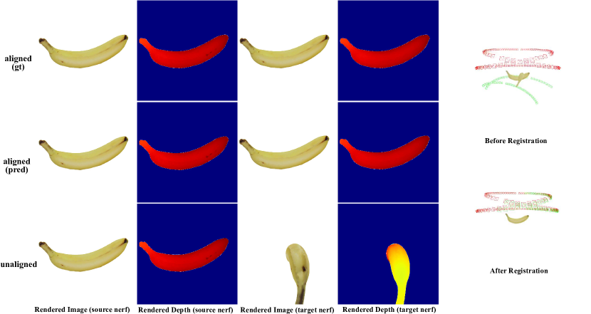
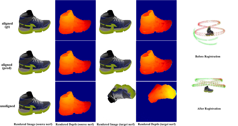
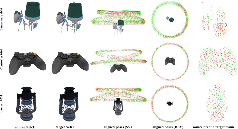
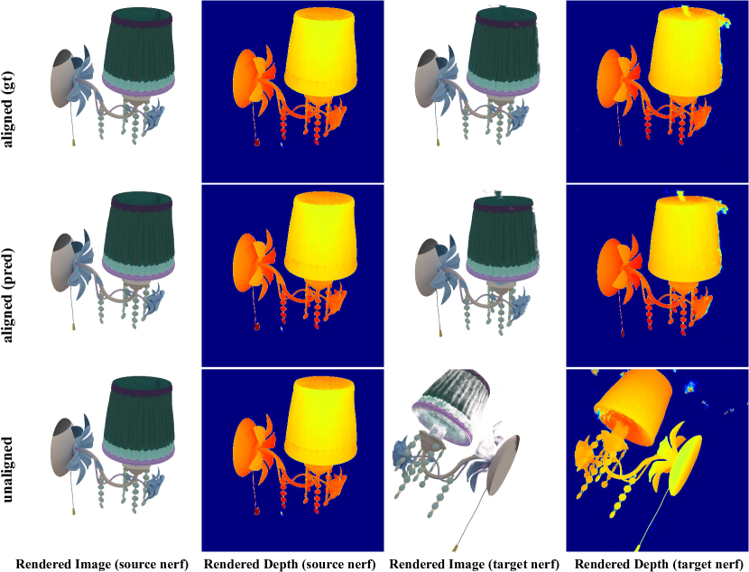
We present some qualitative results in Fig. 4. To visualize the rendered images, we first transform the camera poses $\mathbf{P}_{\text{source}}$ in the source NeRF model to the target NeRF and obtain the transformed camera poses $\mathbf{P}_{\text{source}}^{{}^{\prime}}$, and then we concatenate the transformed camera poses with the camera poses in target NeRF $\mathbf{P}_{\text{render}}=\text{concat}([\mathbf{P}_{\text{source}}^{{}^{\prime}},\ \mathbf{P}_{\text{target}}])$. We use $\mathbf{P}_{\text{source}}$ as the camera trajectories to synthesize images for the target NeRF model. Similarly, we use $\mathbf{P}_{\text{render}}^{{}^{\prime}}=\text{concat}([\mathbf{P}_{\text{source}},\ \mathbf{P}_{\text{target}}^{{}^{\prime}}])$ for the source NeRF model to synthesize images, where $\mathbf{P}_{\text{target}}^{{}^{\prime}}$ is the transformed camera poses from target NeRF to source NeRF. The results are respectively given in columns 1 and 2. We also visualize the aligned camera poses $\mathbf{P}_{\text{render}}$ in column 3 and 4. The red and green color respectively denotes the camera poses aligned by ground truth and our estimated transformations. Moreover, we transform the source prediction to the target coordinate frame and visualize the result in the last column. We further use ground truth transformation to align the camera poses to obtain $\mathbf{P}_{\text{render}}^{\text{gt}}$, and simply concatenate source and target camera poses together to obtain $\mathbf{P}_{\text{render}}^{\text{no trans}}$. Subsequently, we provide the target NeRF respectively with $\mathbf{P}_{\text{render}}^{\text{gt}},\mathbf{P}_{\text{render}},\mathbf{P}_{\text{render}}^{\text{no trans}}$ to render RGB images and depth images. Some of the results are shown in Fig. 6.

Figure 6: View synthesis comparison on object ‘Lampshade a166’. Top row: results from ground truth transformation. Middle row: results from the predicted transformation. Bottom row: results without applying any transformations.

Ablation Studies.

We further show the mean of RRE and RTE in Tab. 3 to ablate our method. “w.o.  conf” denotes training our method without the confidence loss, “w.o.  sf” denotes training our network without the surface field loss, “$\text{Ours}_{\text{df}}$” denotes our method with the surface fields replaced by the density fields. We can see that the surface fields are critical to our network training.

	FGR [46]	REGTR [43]	w.o.  conf	w.o.  sf	$\text{Ours}_{\text{df}}$	Ours
$\Delta\mathbf{R}\ (^{\circ})$	61.59	113.78	71.84	101.17	86.22	9.67
$\Delta\mathbf{t}\ (\times 1e2)$	13.50	43.31	12.97	20.35	16.06	3.85

Table 3: Ablations studies of our method. The results are averaged on the 44 test objects.

Performance Analysis.

To accelerate the network training, we do not query the NeRF model to obtain the voxel grid. Instead, we pre-compute the voxel grids $\mathbf{G}$ and the corresponding binary mask $\mathbf{M}$ for all NeRF blocks and store them on disks. The voxel grid $\mathbf{G}$ and binary mask $\mathbf{M}$ are loaded into memory at each iteration. During training, our network takes about $2.8$ seconds per iteration. The bottleneck on the training time is from loading $\mathbf{G}$, $\mathbf{M}$, and the source and target NeRF models. During inference, our model takes about $0.4$ seconds with the input voxel grid containing about $10$K points. Further acceleration can be achieved by pre-downsampling the voxel grid to a lower resolution.

4.1 Further Discussion

Limitations.

Our method has shown good performance in registering NeRF blocks. However, registering NeRF is still a challenging problem in large-scale scenes. We summarize the limitations of our work as follows (more discussions are given in the supplementary):

• Generalizability vs. out-of-distribution (OOD). While our method is generalizable to unseen in-distribution scenes during testing, we postulate that performance would drop when tested on OOD scenes/object classes, e.g., training on indoor and testing on outdoor scenes, etc.

• Application to real-world data $\&$ unbounded scenes. We emphasize that our training data contains real-world objects (e.g. Shoes in Fig. 3). Our method currently cannot be applied to unbounded scenes since NeRF is not good at geometry estimation. Consequently, incorrect geometries like floaters can influence the performance of our model. It means that our method can fail if the extracted occupancy grid contains too many noisy points (See Fig. 5). We argue that better results can be obtained by applying RANSAC [12] to filter outliers based on our predicted correspondences, or training better NeRF blocks by utilizing depth supervision [11, 30], or utilizing a robust loss [32] to ignoring floaters during training NeRF blocks. In addition, for real-world data that contain background, techniques like [3] can also be applied to our method to get the interested objects. We leave this as our future work.

• Scale in the relative transformation. We follow the assumption of NeRF2NeRF that the scales for two NeRFs are the same, which can be violated in real-world settings. Nonetheless, additional sensors such as IMU, wheel encoders, etc., are easily available to get the absolute scale. For settings where only RGB images are available, the scale can be a problem. Additional scene priors are needed to fix the scale for RGB images as input.

Why localization methods based on SfM tools are not compared?

A simple solution is to first synthesize images using NeRF. We can then use SfM to get 2D-2D correspondences from keypoints matcher and do triangulation to recover the 3D scene points. Consequently, localization-based methods such as perspective-n-points (PnP) [18] or iterative closest point (ICP) [2, 6] can be applied on the 3D scene points to register the NeRF models. However, we argue that SfM is fragile in scenes where keypoint correspondences are difficult to establish. One failure case is given in Fig. 7. As a result, all methods that rely on keypoint correspondences can potentially fail due to wrong matches. Particularly, it is often hard to obtain enough matches for texture-less scenes/objects. False matches can also occur due to changes in image appearance. We circumvent this problem by learning the correspondences from NeRF representations, i.e. the density field, which is shown robust to image appearance changes in the experiments. Moreover, our method is an end-to-end solution and therefore can be much faster than other methods that rely on keypoints, e.g., iNeRF [23] takes more than 50 secs to register an image in an existing NeRF model (c.f. Fig. 4 of the iNeRF paper), while ours only takes 0.4 secs to register two NeRFs.

Figure 7: COLMAP failed on synthetic dataset due to wrong correspondences.

Why not register images in the same coordinate frame by global bundle adjustment (BA)?

We argue that there are cases where using BA to recover all poses may not be the best option:

• Robustness. BA relies on good keypoint correspondences which can be challenging to obtain in texture-less scenes, etc. In contrast, our DReg-NeRF leverages NeRF features for registration without explicit correspondence search on the images.

• Scalability and efficiency. Images of a large scene can be collected in smaller batches. It is more scalable and efficient to build smaller NeRF models on each batch of images and subsequently do NeRF registration to get the NeRF model of the full scene.

• Modularity. It is easier to update a modular NeRF model. Any module can be easily replaced or added via NeRF registration.

5 Conclusion

In conclusion, we have proposed a novel network architecture that registers NeRF blocks into the same coordinate frame. Unlike existing methods, our method does not rely on any initialization and human-annotated keypoints. We constructed a dataset with $1,700+$ objects where images are rendered from 3D textured meshes of the Objaverse dataset. We train our method on our constructed dataset. Our method surpasses the state-of-the-art traditional and learning-based point cloud registration methods when evaluated on the test set.

Acknowledgement.

This research work is supported by the Agency for Science, Technology and Research (A*STAR) under its MTC Programmatic Funds (Grant No. M23L7b0021).

6 APPENDIX

6.1 NeRF Network Architecture

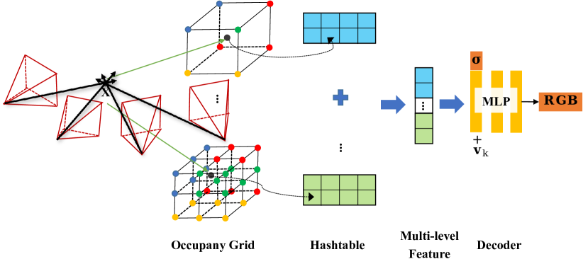
We present the network architecture of our used NeRF network in Fig. 8. The resolution level is 16. The number of hash table entries in each level is $2^{19}$, where the feature dimension of each hash table entry is 2. The coarsest level is 16. We use NeRFAcc [19] to train NeRF models, where only a single resolution occupancy grid is used to skip empty space instead of multi-resolution occupancy grids as in the original InstantNGP implementation.

Figure 8: Network architecture of our used NeRF. A single-resolution occupancy grid is used to skip empty space. The dimension of each hidden layer is 64. The view direction is concatenated with the feature embedding after the first hidden layer without applying positional encodings.

6.2 More Qualitative Results

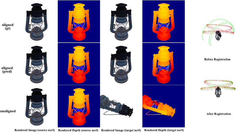
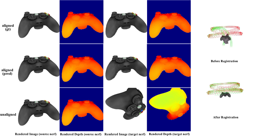
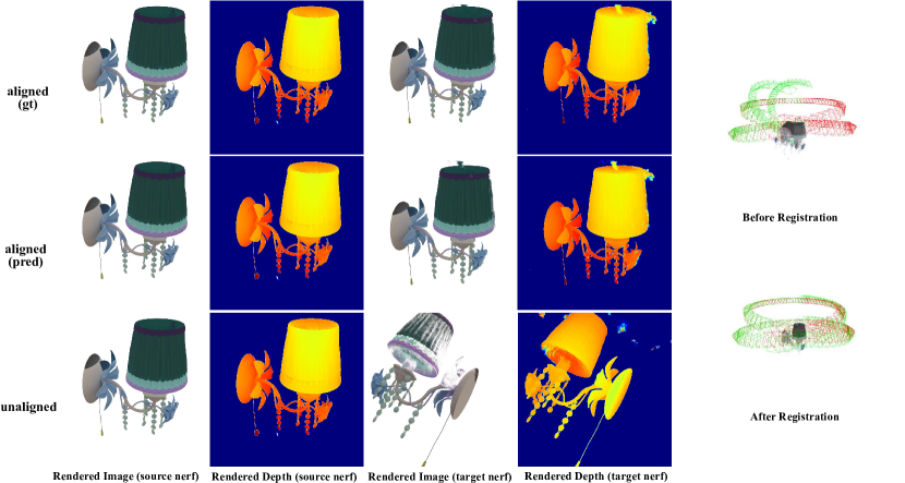
We present more qualitative results in Fig. 9. We further visualize the rendered RGB images and depth images in Fig. 10, Fig. 11 and Fig. 12. In the left part of each figure, we visualize the rendered RGB images and depth images, where the top row shows results from the ground truth transformation, the middle row shows results from the predicted transformation, and the bottom row shows results without applying transformation. The right part of each figure presents camera poses and occupancy grids before registration on the top row, and the camera poses and occupancy grids after registration on the bottom row.

Figure 9: The qualitative results on Objaverse [10] dataset after NeRF registration. From left to right are respectively the rendered images by the source NeRF model, the rendered images by the target NeRF model, the side view (SV) of the aligned camera poses, the birds-eye-view (BEV) of the aligned camera poses, the concatenated predictions by transforming the source prediction to the target NeRF’s coordinate frame. red and green, respectively, denote the results from source NeRF and target NeRF.

Figure 10: View synthesis comparison. Left: (1) Top row: results from ground truth transformation; (2) Middle row: results from the predicted transformation; (3) Bottom row: results without applying the transformation. Right: (1) Camera poses and occupancy grids before registration; (2) Camera poses and occupancy grids after registration.

Figure 11: View synthesis comparison on object. Left: (1) Top row: results from ground truth transformation; (2) Middle row: results from the predicted transformation; (3) Bottom row: results without applying the transformation. Right: (1) Camera poses and occupancy grids before registration; (2) Camera poses and occupancy grids after registration.

Figure 12: View synthesis comparison. Left: (1) Top row: results from ground truth transformation; (2) Middle row: results from the predicted transformation; (3) Bottom row: results without applying the transformation. Right: (1) Camera poses and occupancy grids before registration; (2) Camera poses and occupancy grids after registration.

References

- [1] Jonathan T. Barron. A general and adaptive robust loss function. In IEEE Conference on Computer Vision and Pattern Recognition, pages 4331–4339, 2019.
- [2] Paul J. Besl and Neil D. McKay. A method for registration of 3-d shapes. IEEE Trans. Pattern Anal. Mach. Intell., 14(2):239–256, 1992.
- [3] Jiazhong Cen, Zanwei Zhou, Jiemin Fang, Wei Shen, Lingxi Xie, Dongsheng Jiang, Xiaopeng Zhang, and Qi Tian. Segment anything in 3d with nerfs. CoRR, abs/2304.12308, 2023.
- [4] Anpei Chen, Zexiang Xu, Andreas Geiger, Jingyi Yu, and Hao Su. Tensorf: Tensorial radiance fields. In Computer Vision - ECCV 2022 - 17th European Conference, volume 13692, pages 333–350, 2022.
- [5] Yu Chen and Gim Hee Lee. Dbarf: Deep bundle-adjusting generalizable neural radiance fields. In Proceedings of the IEEE/CVF Conference on Computer Vision and Pattern Recognition, pages 24–34, 2023.
- [6] Yang Chen and Gérard G. Medioni. Object modelling by registration of multiple range images. Image Vis. Comput., 10(3):145–155, 1992.
- [7] Yu Chen, Shuhan Shen, Yisong Chen, and Guoping Wang. Graph-based parallel large scale structure from motion. Pattern Recognition., 107:107537, 2020.
- [8] Yu Chen, Zihao Yu, Shu Song, Tianning Yu, Jianming Li, and Gim Hee Lee. Adasfm: From coarse global to fine incremental adaptive structure from motion. In 2023 IEEE International Conference on Robotics and Automation (ICRA), pages 2054–2061, 2023.
- [9] Yu Chen, Ji Zhao, and Laurent Kneip. Hybrid rotation averaging: A fast and robust rotation averaging approach. In IEEE Conference on Computer Vision and Pattern Recognition, pages 10358–10367, 2021.
- [10] Matt Deitke, Dustin Schwenk, Jordi Salvador, Luca Weihs, Oscar Michel, Eli VanderBilt, Ludwig Schmidt, Kiana Ehsani, Aniruddha Kembhavi, and Ali Farhadi. Objaverse: A universe of annotated 3d objects. CoRR, abs/2212.08051, 2022.
- [11] Kangle Deng, Andrew Liu, Jun-Yan Zhu, and Deva Ramanan. Depth-supervised nerf: Fewer views and faster training for free. In IEEE/CVF Conference on Computer Vision and Pattern Recognition, pages 12872–12881, 2022.
- [12] Martin A. Fischler and Robert C. Bolles. Random sample consensus: A paradigm for model fitting with applications to image analysis and automated cartography. Commun. ACM, 24(6):381–395, 1981.
- [13] Sara Fridovich-Keil, Alex Yu, Matthew Tancik, Qinhong Chen, Benjamin Recht, and Angjoo Kanazawa. Plenoxels: Radiance fields without neural networks. In IEEE/CVF Conference on Computer Vision and Pattern Recognition, pages 5491–5500, 2022.
- [14] Lily Goli, Daniel Rebain, Sara Sabour, Animesh Garg, and Andrea Tagliasacchi. nerf2nerf: Pairwise registration of neural radiance fields. CoRR, abs/2211.01600, 2022.
- [15] Kaiming He, Xiangyu Zhang, Shaoqing Ren, and Jian Sun. Deep residual learning for image recognition. In 2016 IEEE Conference on Computer Vision and Pattern Recognition, pages 770–778, 2016.
- [16] Shengyu Huang, Zan Gojcic, Mikhail Usvyatsov, Andreas Wieser, and Konrad Schindler. Predator: Registration of 3d point clouds with low overlap. In IEEE Conference on Computer Vision and Pattern Recognition, pages 4267–4276, 2021.
- [17] Diederik P. Kingma and Jimmy Ba. Adam: A method for stochastic optimization. In 3rd International Conference on Learning Representations, 2015.
- [18] Laurent Kneip, Davide Scaramuzza, and Roland Siegwart. A novel parametrization of the perspective-three-point problem for a direct computation of absolute camera position and orientation. In IEEE Conference on Computer Vision and Pattern Recognition, pages 2969–2976, 2011.
- [19] Ruilong Li, Matthew Tancik, and Angjoo Kanazawa. Nerfacc: A general nerf acceleration toolbox. CoRR, abs/2210.04847, 2022.
- [20] Tianyang Li, Jian Wang, and Tibing Zhang. L-DETR: A light-weight detector for end-to-end object detection with transformers. IEEE Access, 10:105685–105692, 2022.
- [21] Chen-Hsuan Lin, Wei-Chiu Ma, Antonio Torralba, and Simon Lucey. BARF: bundle-adjusting neural radiance fields. In 2021 IEEE/CVF International Conference on Computer Vision, pages 5721–5731, 2021.
- [22] Tsung-Yi Lin, Piotr Dollár, Ross B. Girshick, Kaiming He, Bharath Hariharan, and Serge J. Belongie. Feature pyramid networks for object detection. In 2017 IEEE Conference on Computer Vision and Pattern Recognition, pages 936–944, 2017.
- [23] Yen-Chen Lin, Pete Florence, Jonathan T. Barron, Alberto Rodriguez, Phillip Isola, and Tsung-Yi Lin. inerf: Inverting neural radiance fields for pose estimation. In IEEE/RSJ International Conference on Intelligent Robots and Systems, pages 1323–1330, 2021.
- [24] Philipp Lindenberger, Paul-Edouard Sarlin, Viktor Larsson, and Marc Pollefeys. Pixel-perfect structure-from-motion with featuremetric refinement. In 2021 IEEE/CVF International Conference on Computer Vision, pages 5967–5977, 2021.
- [25] Lingjie Liu, Jiatao Gu, Kyaw Zaw Lin, Tat-Seng Chua, and Christian Theobalt. Neural sparse voxel fields. In Advances in Neural Information Processing Systems 33, 2020.
- [26] Ilya Loshchilov and Frank Hutter. Decoupled weight decay regularization. In 7th International Conference on Learning Representations, 2019.
- [27] Ben Mildenhall, Pratul P. Srinivasan, Matthew Tancik, Jonathan T. Barron, Ravi Ramamoorthi, and Ren Ng. Nerf: Representing scenes as neural radiance fields for view synthesis. In Computer Vision - ECCV 2020 - 16th European Conference, volume 12346, pages 405–421, 2020.
- [28] Thomas Müller, Alex Evans, Christoph Schied, and Alexander Keller. Instant neural graphics primitives with a multiresolution hash encoding. ACM Trans. Graph., 41(4):102:1–102:15, 2022.
- [29] Casey Peat, Oliver Batchelor, Richard D. Green, and James Atlas. Zero nerf: Registration with zero overlap. CoRR, abs/2211.12544, 2022.
- [30] Barbara Roessle, Jonathan T. Barron, Ben Mildenhall, Pratul P. Srinivasan, and Matthias Nießner. Dense depth priors for neural radiance fields from sparse input views. In IEEE/CVF Conference on Computer Vision and Pattern Recognition, pages 12882–12891, 2022.
- [31] Radu Bogdan Rusu, Nico Blodow, and Michael Beetz. Fast point feature histograms (FPFH) for 3d registration. In 2009 IEEE International Conference on Robotics and Automation, pages 3212–3217, 2009.
- [32] Sara Sabour, Suhani Vora, Daniel Duckworth, Ivan Krasin, David J. Fleet, and Andrea Tagliasacchi. Robustnerf: Ignoring distractors with robust losses. CoRR, abs/2302.00833, 2023.
- [33] Paul-Edouard Sarlin, Daniel DeTone, Tomasz Malisiewicz, and Andrew Rabinovich. Superglue: Learning feature matching with graph neural networks. In 2020 IEEE/CVF Conference on Computer Vision and Pattern Recognition, pages 4937–4946, 2020.
- [34] Andrea Tagliasacchi and Ben Mildenhall. Volume rendering digest (for nerf). CoRR, abs/2209.02417, 2022.
- [35] Matthew Tancik, Vincent Casser, Xinchen Yan, Sabeek Pradhan, Ben P. Mildenhall, Pratul P. Srinivasan, Jonathan T. Barron, and Henrik Kretzschmar. Block-nerf: Scalable large scene neural view synthesis. In IEEE/CVF Conference on Computer Vision and Pattern Recognition, pages 8238–8248, 2022.
- [36] Hugues Thomas, François Goulette, Jean-Emmanuel Deschaud, and Beatriz Marcotegui. Semantic classification of 3d point clouds with multiscale spherical neighborhoods. In 2018 International Conference on 3D Vision, 3DV 2018, pages 390–398, 2018.
- [37] Hugues Thomas, Charles R. Qi, Jean-Emmanuel Deschaud, Beatriz Marcotegui, François Goulette, and Leonidas J. Guibas. Kpconv: Flexible and deformable convolution for point clouds. In 2019 IEEE/CVF International Conference on Computer Vision, pages 6410–6419, 2019.
- [38] Haithem Turki, Deva Ramanan, and Mahadev Satyanarayanan. Mega-nerf: Scalable construction of large-scale nerfs for virtual fly- throughs. In IEEE/CVF Conference on Computer Vision and Pattern Recognition, pages 12912–12921, 2022.
- [39] Shinji Umeyama. Least-squares estimation of transformation parameters between two point patterns. IEEE Trans. Pattern Anal. Mach. Intell., 13(4):376–380, 1991.
- [40] Aäron van den Oord, Yazhe Li, and Oriol Vinyals. Representation learning with contrastive predictive coding. CoRR, abs/1807.03748, 2018.
- [41] Ashish Vaswani, Noam Shazeer, Niki Parmar, Jakob Uszkoreit, Llion Jones, Aidan N. Gomez, Lukasz Kaiser, and Illia Polosukhin. Attention is all you need. In Advances in Neural Information Processing Systems, pages 5998–6008, 2017.
- [42] Yue Wang and Justin Solomon. Deep closest point: Learning representations for point cloud registration. In 2019 IEEE/CVF International Conference on Computer Vision, pages 3522–3531, 2019.
- [43] Zi Jian Yew and Gim Hee Lee. REGTR: end-to-end point cloud correspondences with transformers. In IEEE/CVF Conference on Computer Vision and Pattern Recognition, pages 6667–6676, 2022.
- [44] Alex Yu, Ruilong Li, Matthew Tancik, Hao Li, Ren Ng, and Angjoo Kanazawa. Plenoctrees for real-time rendering of neural radiance fields. In 2021 IEEE/CVF International Conference on Computer Vision, pages 5732–5741, 2021.
- [45] Andy Zeng, Shuran Song, Matthias Nießner, Matthew Fisher, Jianxiong Xiao, and Thomas A. Funkhouser. 3dmatch: Learning local geometric descriptors from RGB-D reconstructions. In 2017 IEEE Conference on Computer Vision and Pattern Recognition, pages 199–208, 2017.
- [46] Qian-Yi Zhou, Jaesik Park, and Vladlen Koltun. Fast global registration. In Bastian Leibe, Jiri Matas, Nicu Sebe, and Max Welling, editors, Computer Vision - ECCV 2016 - 14th European Conference, volume 9906 of Lecture Notes in Computer Science, pages 766–782.