On Gradient-like Explanation under a Black-box Setting:
When Black-box Explanations Become as Good as White-box

Abstract

Attribution methods shed light on the explainability of data-driven approaches such as deep learning models by revealing the most contributing features to decisions that have been made. A widely accepted way of deriving feature attributions is to analyze the gradients of the target function with respect to input features. Analysis of gradients requires full access to the target system, meaning that solutions of this kind treat the target system as a white-box. However, the white-box assumption may be untenable due to security and safety concerns, thus limiting their practical applications. As an answer to the limited flexibility, this paper presents GEEX (gradient-estimation-based explanation), an explanation method that delivers gradient-like explanations under a black-box setting. Furthermore, we integrate the proposed method with a path method. The resulting approach iGEEX (integrated GEEX) satisfies the four fundamental axioms of attribution methods: sensitivity, insensitivity, implementation invariance, and linearity. With a focus on image data, the exhaustive experiments empirically show that the proposed methods outperform state-of-the-art black-box methods and achieve competitive performance compared to the ones with full access.

1 Introduction

Explainability is an increasingly important research topic due to the breakthroughs led by rapidly developing deep learning. Owing to the growth of hardware’s computational powers, deep learning models with growing capacities are able to handle tasks in real-world scenarios. And they may even outperform human experts in certain domains. As data-driven models, deep learning solutions at the current stage are distinguished from traditional approaches based on expert systems (?). The data-driven solutions learn the decision rules implicitly from the given data distribution, which conceals decision reasoning from humans. And it would be risky if the stakeholders have no knowledge about what is happening inside an AI box. For example, previous research (?; ?) reveals the widely existing Clever-Hans-Effect (?). In the context of machine learning, the effect refers to data-driven models learning to use irrelevant features as shortcuts for classification from an unbalanced data distribution (e.g., watermarks only contained in certain classes of instances because of different data sources). Although models suffering from Clever-Hans-Effect may perform well in laboratories, their outcomes are totally unreliable in practice. In addition to the unintentional failure, it has been shown that data-driven models are fragile under adversarial attacks, which steer model outputs by adding artifacts to the targeted input. Employment of these opaque components in crucial application scenarios, such as medical image classification and autonomous driving, can cause unpredictable consequences as they may fail accidentally or intentionally. Explainability, a key to the mysterious box of AI and a potential shield against adversarial attacks (?; ?), is particularly interested in how or why models make up their minds.

Existing explanation methods can be categorized as white-box or black-box methods depending on whether they assume internal access to the explaining target. Regardless of the different settings, both aim to identify the paramount features as explanations for model’s decisions. The latter category was popular at the earlier stage of XAI (explainable AI) research. Methods of this kind are typically applicable to explain outcomes of arbitrary AI models. They prepare a list of queries and explain the decision by analyzing the correlation between the inputs and outputs. Although they are still widely adopted due to their flexibility benefiting from the loosened assumption about model access, their popularity is overtaken by white-box approaches. The reason behind this is the shifted research interest of the deep learning community towards higher dimensional data like images and texts. The computational expense of black-box methods, which explain through a substantial amount of queries, becomes unaffordable in the enlarged search space while dealing with high-dimensional data.

As the name implies, white-box explanation methods assume full access to the target model. Given more details about the inference procedure, they produce precise explanations by investigating the gradient/information flow throughout the target. In practice, however, there is no guarantee of detailed internal access to models due to safety and security concerns, which limits their applications in real-world scenarios. Flexibility is another concern. Modifications are needed when a white-box approach is applied to explain other models that its original design does not consider. One should not expect a gradient-based approach examining neural networks with backward propagation to uncover the inference process of a tree-based model without adjustments.

Focusing on image data, this paper presents Gradient-Estimation-based EXplanation (GEEX), an explanation method delivering gradient-like explanations under a black-box setting. It is exempted from the full access assumption and can be applied to arbitrary models in principle. This property makes GEEX an alternative for explainability under circumstances where details about the target are unavailable. Compared to other black-box explainers, GEEX fine-grinds feature attributions, thus enabling the explanation outputs to highlight smaller and distributed features with homologous structures to gradient-based explanations rather than a few fuzzy hot regions. Similar to gradient-based approaches, although GEEX breaks the Sensitivity axiom, combining its estimation kernel with a path method overcomes the limitation. The resulting method iGEEX fulfills the four fundamental axioms of attribution methods (?), i.e. Sensitivity, Insensitivity, Implementation Invariance, and Linearity.

2 Related work

Black-box, or model-agnostic, explanation methods are applicable to arbitrary AI models in principle. They treat the to-be-explained model as a black-box with its internal functions left out. The general ideas behind methods of this kind are similar: creating a synthetic set by altering the original input $x$, then deriving the explanation for the decision $f(x)$ through analysis of the correlation between changes in the inputs and outputs. LIME (?) is one of the most representative methods from this category. It first simplifies the input features as a binary vector, then generates the synthetic set by randomly switching on/off features. For image data, an additional step conducted by LIME is clustering pixels as superpixels according to the similarity of pixel values and their spatial distances (?), which reduces the search space to a user-defined size. Simplifying the search space enables LIME to highlight wider regions where the important features locate.

Apparently, grouping pixels can negatively affect explanation quality. It has been shown that low-level features such as edges and contours are considered informative to classification problems by current deep learning models (?). Superpixel techniques possess the risk of breaking low-level features into diverse components as they inevitably segment pixels along edges. Consequently, the explanation method may overlook (part of) the divided features or include irrelevant pixels. RISE (?) adopts mask resizing that overcomes the challenge. More specifically, it generates smaller initial masks and upsamples them to the target size by performing bilinear interpolation. By doing so, RISE is capable of handling any shape of low-level features without expanding the search space, which significantly improves explanation quality.

Compared to black-box methods, more efforts have been spent on white-box approaches while explaining image classifiers as they sharpen resultant attribution maps owing to the detailed access to the target. The most straightforward white-box approach directly adopts vanilla gradients (?) as explanations. It traces the partial derivative of the decision function with respect to the input backward throughout the model. However, previous work (?) shows that explanations based on vanilla gradients can contain heavy noises. A potential cause of this observation is the rapid derivative fluctuation at small scales (?).

SmoothGrad (?) smooths explanation outcomes by applying a Gaussian kernel to the input and averaging over the acquired gradients. Such a process has a robust denoising effect that positively correlates to the number of samples used during smoothing. Apart from being a standalone solution for explainability, one can also plug SmoothGrad into other gradient-based approaches for smoothing purposes. Similarly, integrated gradients (IG) denoises explanations by integrating derivatives from multiple queries over a path (?). For any input, IG interpolates between the original instance and the pre-defined baseline (usually a zero matrix) to generate queries. The interpolation interval determines the number of queries to integrate. Alternatively, the group of propagation-based methods (?; ?) nails the denoising challenge by means of propagation rules, which explicitly utilize model structures and complete the explanation process with one single round-trip.

3 Gradient Estimation for Explanation

This section details the proposed method GEEX. For any decision $f(x)$ made by a target model on an input $x$, the goal of GEEX is to determine the feature attribution $\xi_{x}$ of that decision under a black-box setting. Here, the black-box setting is defined by query access, assuming only access to the inputs and outputs of a model, with all details about the inference procedure hidden. Such a setting has practical meanings as model accessibility can be limited under the deployment environment due to, for example, model owner concerns about security and plagiarism. Compared to the white-box setting, the black-box setting has a loosened constraint on the accessibility of the model. But the main challenge of deriving gradient-based explanations without internal access is the lack of directly available gradients. Luckily, there are possibilities to estimate gradients through queries. We adopt natural evolution strategies for gradient estimation as a walk around to the unavailable gradients.

Natural Evolution Strategies

Natural evolution strategies (NES) are algorithms designed for black-box optimization problems (?), which are widely utilized in reinforcement learning (?). Instead of propagating gradients backward along neuron connections, NES estimates gradients with a search distribution determined by the parameters of interest. It defines gradients as the direction towards lower expected loss with respect to the analyzing target, namely the input $x$ in the context of explainability. Denoting the loss function by $\mathcal{L}(\cdot)$ and the current set of parameters by $x$, the expected loss over the search distribution can be written as follows (?):

$$J(x)=\mathbb{E}_{x}[\mathcal{L}(f(z))]=\int\mathcal{L}(f(z))\pi(z|x)~{}\mathrm{d}z$$

where $\pi(\cdot|x)$ indicates the search distribution parameterized by $x$ and $z$ denotes instance sampled from the given distribution. Please note that we denote the parameter set with $x$ to emphasize that the analysis target is the input features rather than the model parameters considered in common settings, which are not available in the case of explaining a black-box. The search gradients with respect to $x$ can be then simplified with the log-likelihood trick:

$$\nabla_{x}J(x) =\nabla_{x}\int\mathcal{L}(f(z))\pi(z|x)~{}\mathrm{d}z$$

$$=\int[\mathcal{L}(f(z))\nabla_{x}\log\pi(z|x)]\pi(z|x)~{}\mathrm{d}z$$

$$=\mathbb{E}_{x}[\mathcal{L}(f(z))\nabla_{x}\log\pi(z|x)]$$

An empirical approximation of the formula above can be acquired with $m$ instances sampled from the search distribution $\{z_{1},z_{2},...,z_{m}\}\sim\pi(\cdot|x)$:

$$\nabla_{x}J(x)\approx\frac{1}{m}\sum_{i=1}^{m}\mathcal{L}(f(z_{i}))\nabla_{x}\log\pi(z_{i}|x)$$ (1)

Theoretically, any differentiable distribution can be a candidate for the search distribution $\pi(\cdot|x)$. Since the distribution of pixel values is not explicitly given, we adopt Gaussian distribution $\mathcal{N}(x,\sigma)$ parameterized by the input $x$ and a pre-defined hyperparameter $\sigma$. The standard deviation $\sigma$ determines the search range. Substituting $\pi(\cdot|x)$ in Equation 1 with Gaussian distribution yields:

$$\xi^{GEEX}_{x}=\nabla_{x}J(x)\approx\frac{1}{m}\sum_{i=1}^{m}\mathcal{L}(f(z_{i}))\frac{x-z_{i}}{\sigma^{2}}$$

Regarding the loss function, it is possible to use the logits of a target class directly as the loss to determine how the changed features affect the prediction confidence on the relevant class. A shortcoming of using logits directly is that the explanations are strongly bounded to the target class. Alternatively, cross-entropy is a better choice to determine features that are considered informative by the model in general. For uncovering the most contributing features, instead of maximizing the probability of the expected class, we are interested in the gradients towards the minimization of useful information for classification. To achieve so, we defined the target probability distribution as the so-called “non-informative” outcome $\hat{y}=\left<\frac{1}{k},\frac{1}{k},...,\frac{1}{k}\right>$, where $k$ is the total number of classes in the classification task. $\mathcal{L}(f(z))=H(\hat{y},f(z))$ returns the cross entropy loss about how informative the predictions are.

Noise Sampling

To create the sample set for explaining a decision $f(x)$ following the distribution $\mathcal{N}(x,\sigma)$, we first sample a set of noise masks from the standard normal distribution $\epsilon\sim\mathcal{N}(0,1)$ and then acquire the synthetic instances by applying noises to the original input $z=x+\sigma\epsilon$. And for every sampled mask $\epsilon$, mirror sampling (?) that adds its symmetric mask $-\epsilon$ to the mask set is applied for estimation robustness. Sampling noise independently from the input allows us to use an identical set of pre-generated noises while explaining different decisions and thus increases explanation efficiency. Besides, it is foreseeable that a carefully selected mask set that maximizes the information gain of each sample can acquire precise estimation with fewer queries, but we leave it as future work and follow the naive sampling process.

However, the naive pixel-wise sampling approach has three limitations when handling high-dimensional inputs:

• Noisy estimation: pixel-wise sampling does not align with the fact that the adjacent pixels are usually correlated. Artifacts (from sampling) with unnatural contrast introduce noises to explanation outcomes.

• Scaling effect: the necessary number of samples for deriving reliable estimations increases exponentially with the rising size of the input.

• Vanishing gradient: inputs with high dimensionality are difficult to be fully masked out by pixel-wise perturbation. When the partially masked features possess enough information for steering the model to its original prediction, vanishing gradients during the estimation will be triggered due to the barely changed outcomes (see proof in Supplement S-I).

Among the three limitations, the third is a particular threat to explaining robust classifiers (e.g. networks with dropout layers or trained with data augmentation).

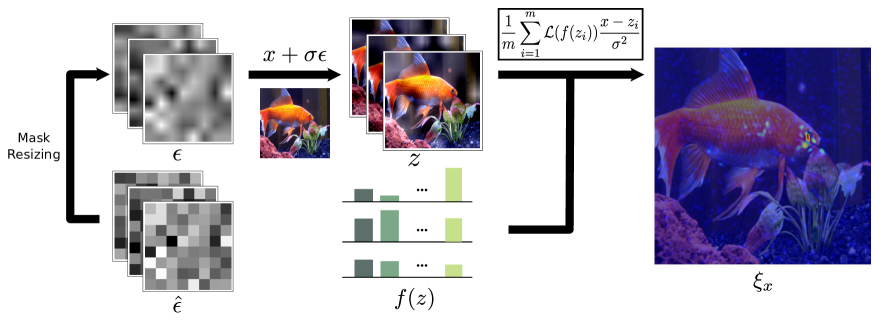
Figure 1: Overview of GEEX. The sample set $\{z_{i}\}$ is constructed by applying the upsampled noises $\epsilon$ from the initial mask set $\hat{\epsilon}$ to the input $x$. The final explanation $\xi_{x}$ (overlaying the original input with the explanation) is derived through the estimation of searching gradients according to the impacts of pixel-wise changes on the prediction outcomes.

Mask resizing (?) tackles all three challenges simultaneously. It first samples noise masks $\hat{\epsilon}$ in reduced feature space with size $\hat{h}\times\hat{w}$ (specified by the user), then performs upsampling with bilinear interpolation to reach the target image size $h\times w$. As a result, the search space is significantly reduced (depending on the resizing ratio). And the smoothed masks (by interpolation) have a denoising effect on the estimated gradients. Most importantly, mask resizing has a higher chance to fully suppress one(several) local feature(s), thus highlighting the gradients by emphasizing the difference among the model outputs. Although mask resizing has the potential to harm the preciseness of explanations, our experiments demonstrate that the advantage brought by solving the above challenges overcomes its downside, especially for inputs with higher dimensions. Fig. 1 summarizes the final estimation scheme including the sampling process.

Integrated Gradient Estimation

So far, we show the possibility of acquiring gradient-like explanations with only query access. Estimated gradients deliver accurate simulations of gradients and reveal information about the inference process. However, similar to other gradient-based approaches, gradient estimation may be trapped by locally flattened segments of a function, thus assigning zero contributions to features that in fact have impacts on the decision. Overlooking relevant features causes the violation of Sensitivity. Vice versa, and most importantly, gradient methods lack a baseline or reference to which the impact of a feature is compared. Attributing contributions to features that have no impact is measured by Insensitivity (called Dummy in (?)). Both fundamentally limit the applicability of gradient methods. Sensitivity and Insensitivity together with so-called Implementation Invariance and Linearity of the explanations (see Supplement S-II) make up a set of four axioms, which describe highly desirable characteristics of attribution methods. Among the four axioms, Sensitivity and Insensitivity directly relate to explanation quality. Violating either of the two will end in misleading results (?).

Path methods are the only attribution methods that satisfy the four axioms all at once (?). Fortunately, GEEX can be converted to a path method if plugged into the explanation scheme of integrated gradients. IG attributes feature contributions using the following form, which integrates the gradients of a set of instances interpolated between the input $x$ and a baseline image $\mathring{x}$:

$$\xi_{x}^{IG}=\frac{(x-\mathring{x})}{s}\circ\sum_{j=1}^{s}\frac{\partial f(x+\frac{j}{s}(x-\mathring{x}))}{\partial x}$$

where $s$ denotes the number of interpolation steps. IG models the absence of features using the baseline $\mathring{x}$, whose explanations demonstrate the importance of feature presence rather than the local sensitivity of the target function to features (raw gradients). Now replacing actual gradients with estimations yields integrated GEEX (iGEEX):

$$\xi_{x}^{iGEEX}=\frac{(x-\mathring{x})}{s}\circ\sum_{j=1}^{s}\xi^{GEEX}_{\mathring{x}+\frac{j}{s}(x-\mathring{x})}$$

Theorem 1.

Integrated GEEX, a path method built upon estimated gradients, satisfies Sensitivity, Insensitivity, and Implementation Invariance. Linearity is also fulfilled when the loss is a linear function of model outcomes.

Please note that the fulfillment of the axioms comes true when enough samples have been drawn, so the statement should be interpreted in a probability sense. The proof and further details of Theorem 1 locate in Supplement S-II.

4 Experiments

With a focus on image data, we test the proposed methods – GEEX and iGEEX with neural networks trained on three popular image datasets. In addition, we include the variant with mask resizing, noted as GERS (gradient estimation with resizing). The experimental environment (hardware and software settings) is described in Supplement S-III.

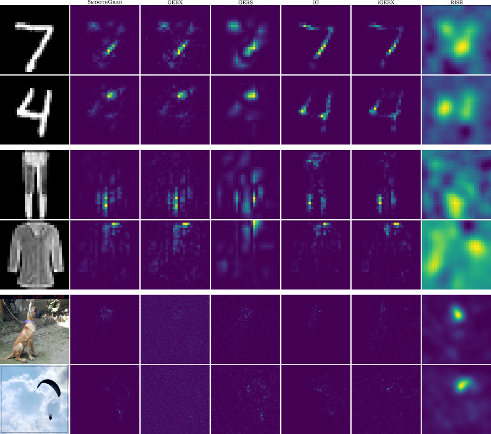
Figure 2: Sample explanations from the selected competitors

Experimental Details

Dataset: We evaluate our approach with models trained on three datasets, namely MNIST (?), Fashion MNIST (?), and ImageNet (?). The selection includes two gray-scale datasets and one full-colored with a significantly larger input size. For each dataset, we train a classifier with its training set and evaluate explanations using the test set.

Classifier: For MNIST and Fashion MNIST, we train a simple CNN model with two convolutional layers, each having a kernel size of 5, concatenated by three dense layers with sizes of 120, 84, and 10. The input sizes of both gray-scale datasets are $28\times 28$. As for ImageNet, we adopt the pre-trained version of Inception V3 (?; ?). The model takes input with size $299\times 299$, which contains roughly a hundred times more pixels than the other two datasets. Through the different input sizes, we demonstrate the impact of the scaling effect on explanation quality.

GEEX: As previously mentioned, we include three variants of the gradient-estimation-based explanation: GEEX, GERS, and iGEEX. The hyperparameter settings are identical for the three variants across all test settings with the number of samples $m$ set to $5k$ and the kernel width $\sigma$ set to $1.0$. The initial mask size of GERS $\hat{h}\times\hat{w}$ is $12\times 12$ for smaller inputs (MNIST and Fashion MNIST) and $80\times 80$ for images from ImageNet. The target mask size equals the original input size. Regarding iGEEX, it uses the vanilla estimation kernel for smaller inputs and involves mask resizing while handling inputs with higher dimensionality for better performance. Its root point for integration is a zero matrix in all test settings. Due to the space limitation, the study on the hyperparameter effects is reported in Supplement S-V.

Competitor: The selection of competitors includes two white-box explanation methods and two black-box methods:

• SmoothGrad (?): a gradient-based approach that averages vanilla gradients of several perturbed versions of the input. Besides, we consider it the baseline due to its direct connection to gradients.

• IG (?): another gradient-based approach that integrates gradients of samples interpolated from the target to a root point (a zero matrix).

• LIME (?): a black-box explanation method that trains a linear classifier in a simplified feature space to mimic the local classification behavior of the target model for deriving explanations.

• RISE (?): a black-box approach derives feature attribution by computing the expected impacts on prediction outcomes for input features.

Comparison to White-box Explanation

We first qualitatively compare GEEX variants to the two white-box approaches. Examples listed in Fig. 2 demonstrate the proximity of explanations from GEEX and GERS to the baseline across different test settings (see more examples in Supplement S-IV). For smaller inputs (the first four rows), GEEX captures homologous attribution structures in comparison to the baseline. Benefiting from the accurate estimation of gradients, iGEEX delivers almost the same results as IG. Both integrate gradients over a straightline path. GERS highlights mostly identical regions, but its saliency maps are relatively fuzzy due to the application of mask resizing. However, the expected denoising effect is barely recognizable while handling smaller inputs as there are few noises observed in explanations with pixel-wise sampling.

The last column of Fig. 2 lists the explanations delivered by RISE as a reference to demonstrate the difference between gradient-based approaches and previous black-box explainers. RISE’s results tend to cover larger regions and therefore overlook features on a smaller scale. Using the third row (the instance classified as “Trouser”) as an example, the first three methods highlight model attribution locating at the gap between the trouser legs, which distinguishes a trouser from a pullover or a dress. But the same observation cannot be obtained from the explanation by RISE.

GEEX nails explanations for decisions on smaller inputs but suffers from noises caused by the scaling effect when feature space expands. As shown by the examples from ImageNet (the last two rows in Fig. 2), although GEEX still identifies relevant pixels that match the actual gradients, the heavy noises make the results visually less accessible. In comparison, GERS successfully suppresses noises through mask resizing and produces results with higher contrast that spots the most contributing features to the decisions. The two path methods agree with the results from the baseline. RISE identifies wider hot regions that cover most of the relevant pixels. But it misses the person attached to the parachute presented by a few pixels in the last example, which is considered relevant by the baseline.

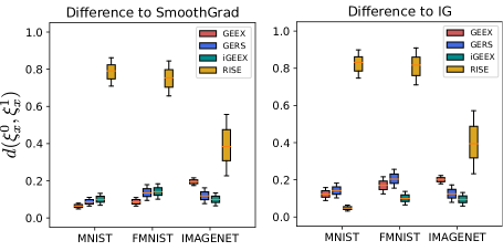
Figure 3: Pixel-wise attribution difference between black-box explanations and gradient-base explanations.

To further quantify the proximity of the estimation to actual gradients, we compute the distance between the explanations from the selected methods and those from the two white-box approaches. For two explanations $\xi_{x}^{0},\xi_{x}^{1}\in\mathbb{R}^{h\times w}$ of the input $x$ from different methods, we compute the distance by $d(\xi_{x}^{0},\xi_{x}^{1})=\frac{||\xi_{x}^{0}-\xi_{x}^{1}||_{1,1}}{h\times w}$, where $||\xi_{x}^{0}-\xi_{x}^{1}||_{1,1}$ denotes the $L_{1,1}$ norm of the difference matrix, namely the sum of the $L_{1}$ norms of columns. Before the computation of differences, explanations from different sources are rescaled in order to align the potentially different scales of various explanation approaches. The normalization process $\tilde{\xi_{x}}=\frac{\xi_{x}}{\mathrm{max}(|\xi_{x}|)}$ rescales an explanation with its maximal element so that the normalized attribution $\tilde{\xi_{x}}$ sticks to the range of $[0,1]$.

Fig. 3 shows the pixel-wise difference in explanations from different sources. The box plot on the left demonstrates the attribution differences between the selected black-box competitors and the baseline, and the right chart shows their differences to IG. Consistent with the analysis of the qualitative examples, explanations from the GEEX family are similar to the results based on actual gradients, whereas RISE assigns feature attribution differently. It was unexpected that, in spite of the noisy backgrounds demonstrated by the sample explanations, GEEX would maintain the explanation similarity at the same level for the ImageNet dataset as in the simpler test scenarios. The reason behind this is the higher ratio of inactive regions shown in all explanations for ImageNet. The massive amount of features having an importance score close to zero lower the mean pixel-wise distances, which also explains the drop in the differences of explanations by RISE. Besides, since there barely exist noises in GEEX’s explanations under the simpler test cases, the downside of mask resizing dominates its impact on explanation quality, which harms the preciseness of gradient estimation. In contrast, along with the rise of noises after switching to a high-dimensional feature space, the denoising effect takes the lead in the trade-off between smoothness and preciseness, which results in higher proximity to the gradient-based explanations.

Quantitative Evaluation for Effectiveness

Table 1: The normalized AOPC scores by evaluation via deletion, higher is better.

Classifier	Dataset	SmoothGrad	IG	RISE	LIME	GEEX	GERS	iGEEX
CNN	MNIST	0.9287	0.9366	0.9158	0.8783	0.9160	0.9176	0.9395
CNN	Fashion MNIST	0.8925	0.8981	0.8777	0.8167	0.8814	0.8764	0.8979
InceptionV3	ImageNet	0.9463	0.9488	0.8878	0.8675	0.9026	0.9449	0.9207
∗The overall best performances are in bold and the highest scores achieved by black-box explainers are underlined.

Lacking the ground truth of explanations makes quantitative evaluation challenging, and there is yet no perfect solution for it. Some work designs human-grounded evaluation procedures (?) that ask a human annotator to rate whether explanation outcomes match their expectations. However, we argue that this approach is inappropriate since an explaining target does not necessarily learn the correct features for classification. Clever-Hans effect, as an example, could drive model attention away from the actual relevant features. In this case, despite the truth that an explanation is against human intuition, it reflects the classification behavior of the target.

Compromising with the absence of explanation ground truth, we use a widely adopted evaluation scheme – evaluation via deletion (?). The motivation is intuitive: hiding the most contributing features should trigger a larger change in prediction results. More specifically, evaluation via deletion removes pixels sequentially in descending order of their feature attributions. Since the common image classifiers cannot handle inputs with absent features, the deletion process replaces the removed pixels with a default value. We set the default value to zero throughout the experiment. After each step of deletion, the evaluation scheme records the changing trend of the prediction confidence for the class that has been decided. We summarize the perturbation curves with normalized AOPC (area over perturbation curve) (?), the cumulative sum of confidence drop ratios after the deletion of pixels, to quantify the performance of the competitors:

$$AOPC=\frac{1}{l}\sum^{l}_{i=1}(1-\frac{f(x^{(i)}}{f(x)}))$$

where $x^{(i)}$ denotes a variant of $x$ with its top-$i$ pixels masked out. AOPC score indicates not only the presence of important features but also whether they are correctly ranked.

Table 1 reports the normalized AOPC scores. The table groups the explanation methods according to their assumptions about model accessibility. Among all competitors, except for SmoothGrad and IG, the rest explain model outcomes under a black-box setting. As shown in the table, methods having internal access to the inference procedure take the lead. However, the three estimation-based approaches highlight themselves with their competitive performances under authority constraints. Furthermore, GEEX and its variants show consistent superiority over the other two black-box approaches.

Within the GEEX group, the application of mask resizing (GERS) makes minor differences in explanation quality while handling smaller inputs. Mask resizing even contributes negatively when tested on Fashion MNIST, because the loss of preciseness outweighs the barely recognizable denoising effect in the lower dimensional feature space. But Consistent with the observation in the qualitative analysis, the accurate estimation of gradients results in similar figures achieved by GEEX, GERS, and the baseline in terms of normalized AOPC score. Leveraging the accurate estimation, IG and iGEEX, which substitutes actual gradients with estimated gradients, are comparable in performance.

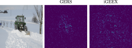
Figure 4: An example of amplified noises after integration.

The improvements brought by mask resizing become significant after switching to a higher dimensional feature space, which is the consequence of solving the three limitations of the pixel-wise sampling approach. Although mask resizing suppresses noises in gradient estimation to a certain extent, the final explanations could still be noisy. Recalling that IG integrates gradients with the formula $\frac{x-\mathring{x}}{s}\sum\frac{\partial f}{\partial x}$, the multiplication of derivative with the difference between the input and the root makes its explanations biased towards pixels, whose values differ the most in both poles of the path (namely pixels with higher values when the root is a zero matrix). The bias towards certain pixels possesses the risk of amplifying noises in estimations (Fig. 4 gives a concrete example), which explains the drop in performance after conducting integration. This observation suggests that the integration of estimated gradients has a strict requirement on the quality of estimations.

LIME, one of the earliest black-box methods, performs relatively humbly. Its dependency on the segmentation results, which inevitably assigns high importance scores to irrelevant features, drags the explanation performance. RISE performs similarly to ours in simpler test scenarios, but becomes less effective for the complicated task. As shown before, RISE tends to have a more concentrated heat map distribution. This property prohibits RISE from identifying small distributed features, which widely exist in advanced classifiers for challenging tasks.

5 Conclusion

In this work, we propose GEEX, a model-agnostic explanation method that derives gradient-like explanations under a black-box setting. Applying mask resizing, its variant GERS addresses the three challenges in high-dimensional feature spaces. Also, we substitute estimated gradients for actual gradients used in IG. The integration of gradient estimations over a path makes the proposed iGEEX consistent with the fundamental properties of attribution methods. Our experimental results qualitatively and quantitatively show the proximity of the estimated gradients to the actual gradients derived from the baseline approach, which outperform other state-of-the-art black-box explainers. Although the experiments focus on image data because of the interest in deriving black-box explanations in high-dimensional feature spaces, we want to note that the same idea is applicable to other data forms, e.g. tabular and textual data.

S-I Vanishing Gradient Caused by Scaling-effect

As stated in Section 3, the failure of the sampling process in demonstrating the output changes will cause vanishing gradients during the estimation, which is a major challenge while explaining inputs from high-dimensional feature space. This conclusion is intuitive and can be easily proved through the formula for gradient estimation:

$$\xi^{GEEX}_{x}=\nabla_{x}J(x)\approx\frac{1}{m}\sum_{i=1}^{m}\mathcal{L}(f(z_{i}))\frac{x-z_{i}}{\sigma^{2}}$$

Proof.

Given a sample set $\mathcal{Z}$, no changes in model outputs indicates:

$$f(z_{i})=f(z_{j}),~{}\forall z_{i},z_{j}\in\mathcal{Z}\iff\mathcal{L}(f(z_{i}))=\mathcal{L}(f(z_{j})),~{}\forall z_{i},z_{j}\in\mathcal{Z}$$

Applying the equality of the losses, we replace $\mathcal{L}(f(z_{i}))$ in the gradient estimation formula with $\mathcal{L}(f(z_{0}))$:

$$\xi^{GEEX}_{x} =\frac{1}{m}\sum_{i=1}^{m}\mathcal{L}(f(z_{0}))\frac{x-z_{i}}{\sigma^{2}}$$

$$=\frac{\mathcal{L}(f(z_{0}))}{m\sigma^{2}}\sum_{i=1}^{m}(x-z_{i})$$

$$=\frac{\mathcal{L}(f(z_{0}))}{m\sigma^{2}}\cdot(mx-\sum_{i=1}^{m}z_{i})$$

For any symmetric distribution, the estimation produces a zero matrix when the sample set size becomes large enough, as $\sum_{i=1}^{m}z_{i}=mx$. Furthermore, mirror sampling adopted by GEEX for the construction of $\mathcal{Z}$ makes the convergence to 0 independent of the size of the sample set. The second term in the bracket can be rewritten as the sum of sample pairs $(z_{i}^{+},z_{i}^{-})$ when mirror sampling applies, where $z_{i}^{+}=x+\epsilon_{i}$ and $z_{i}^{-}=x-\epsilon_{i}$:

$$=\frac{\mathcal{L}(f(z_{0}))}{m\sigma^{2}}\cdot(mx-\sum_{i=1}^{m/2}(z_{i}^{+}+z_{i}^{-}))$$

$$=\frac{\mathcal{L}(f(z_{0}))}{m\sigma^{2}}\cdot(mx-\frac{m}{2}\cdot 2x)$$

$$\implies\xi^{GEEX}_{x} =0$$

∎

S-II Proof of Satisfaction on the Four Axioms

Proposition 1 states that iGEEX fulfills the four fundamental axioms of attribution methods. This section gives the proof of these properties one by one.

Axiom: Implementation Invariance

For any two functionally equivalent models, Implementation Invariance indicates that the explanations for the decisions made by the two models ought to be identical despite the different implementations. Apparently, all black-box approaches, including GEEX and iGEEX, satisfy Implementation Invariance as they only concern outputs of target functions and omit implementation details during the explanation process.

Axiom: Sensitivity

Sensitivity states that if the input and the baseline differing in one feature receive different predictions, then the differing feature should be assigned a non-zero importance score. Previous work has shown that gradient-based approaches (including GEEX) break Sensitivity, yet, iGEEX satisfies this axiom.

Proof.

Focusing on the one feature $x_{(k)}$, whose value differs between the input and the root, the model attribution on this specific feature produced by GEEX is $\xi_{x_{(k)}}^{GEEX}=\frac{\partial J}{\partial x_{(k)}}|_{x}$. The assigned attribution can be 0 when the loss function is locally flattened. Substituting the actual gradients in IG by the estimation kernel recovers Sensitivity:

$$\xi_{x_{(k)}}^{iGEEX} =\frac{(x_{(k)}-\mathring{x}_{(k)})}{s}\sum_{j=1}^{s}\xi^{GEEX}_{\mathring{x}+\frac{j}{s}(x-\mathring{x})}=\frac{(x_{(k)}-\mathring{x}_{(k)})}{s}\sum_{j=1}^{s}\frac{\partial J}{\partial x_{(k)}}|_{\mathring{x}+\frac{j}{s}(x-\mathring{x})}$$

$$=(x_{(k)}-\mathring{x}_{(k)})\mathbb{E}[\frac{\partial J}{\partial x_{(k)}}]$$

$$=J(x)-J(\mathring{x})\neq 0$$

∎

Axiom: Insensitivity

Insensitivity (Dummy) means: for the features that the target function does not dependent on, then the attributions of those features are zero. The premise of the fulfillment of iGEEX is that IG fulfills Insensitivity, i.e.:

$$\int_{0}^{1}\frac{\partial\mathcal{L}(f(x_{\alpha}))}{\partial x_{\alpha}}d\alpha=0$$ (2)

where $x_{\alpha}=\alpha\mathring{x}+(1-\alpha)x$ is an interpolated instance between $x$ and $\mathring{x}$. To prove the Insensitivity of iGEEX, we show below that $\xi^{iGEEX}_{x_{(k)}}$ converges to 0 when the sample set becomes large enough.

Proof.

We first expand the expression of the estimation kernel in iGEEX:

$$\xi_{x}^{iGEEX} =\frac{(x-\mathring{x})}{s}\circ\sum_{j=1}^{s}\xi^{GEEX}_{\mathring{x}+\frac{j}{s}(x-\mathring{x})}=\frac{(x-\mathring{x})}{s}\circ\sum_{j=1}^{s}\Biggl{[}\frac{1}{m}\sum_{i=1}^{m}\mathcal{L}(f(z_{ji}))\frac{x_{j}-z_{ji}}{\sigma^{2}}\Biggr{]}$$

$${=}\frac{(\mathring{x}-x)}{s}\circ\sum_{i=1}^{m}\sum_{j=1}^{s}\mathcal{L}(f(z_{ji}))\frac{\epsilon_{i}}{m\cdot\sigma^{2}}$$

Concentrating on the k-th feature that should have a zero attribution score yields:

$$\xi^{iGEEX}_{x_{(k)}} =\frac{(\mathring{x}_{(k)}-x_{(k)})}{s}\sum_{i=1}^{m}\sum_{j=1}^{s}\mathcal{L}(f(z_{ji}))\frac{\epsilon_{i(k)}}{m\cdot\sigma^{2}}$$

$$=\frac{(\mathring{x}_{(k)}-x_{(k)})}{s\sigma^{2}}\sum_{i=1}^{m}\frac{\epsilon_{i(k)}}{m}\sum_{j=1}^{s}\mathcal{L}(f(x_{j}+\epsilon_{i}))$$

Here, the element-wise product is simplified as the product of two values. Analogous to the notion $x_{(k)}$ for the k-th feature of an instance, we denote the k-th element of a mask $\epsilon_{i}$ from the mask set by $\epsilon_{i(k)}$. Please note that rather than the k-th element $\epsilon_{i(k)}$, it is the full mask $\epsilon_{i}$ that is applied to the input for computing the expected loss even when we focus solely on the attribution of the k-th feature. The loss can be expanded with the Taylor series:

$$\mathcal{L}(f(x_{j}+\epsilon_{i}))=\mathcal{L}(f(x_{j}))+\nabla\mathcal{L}(f(x_{j}))^{T}\cdot\epsilon_{i}+O(||\epsilon_{i}||^{2})$$

Now we rewrite $\xi_{x_{(k)}}^{iGEEX}$ as:

$$\xi^{iGEEX}_{x_{(k)}} =\frac{(\mathring{x}_{(k)}-x_{(k)})}{s\sigma^{2}}\sum_{i=1}^{m}\frac{\epsilon_{i(k)}}{m}\sum_{j=1}^{s}[\mathcal{L}(f(x_{j}))+\nabla\mathcal{L}(f(x_{j}))^{T}\cdot\epsilon_{i}+O(||\epsilon_{i}||^{2})]$$

$$=\frac{(\mathring{x}_{(k)}-x_{(k)})}{s\sigma^{2}}\Biggl{[}\underbrace{\sum_{i=1}^{m}\frac{\epsilon_{i(k)}}{m}\sum_{j=1}^{s}\mathcal{L}(f(x_{j}))}_{\Circled{1}}+\underbrace{\sum_{i=1}^{m}\frac{\epsilon_{i(k)}}{m}\sum_{j=1}^{s}\nabla\mathcal{L}(f(x_{j}))^{T}\cdot\epsilon_{i}}_{\Circled{2}}+\underbrace{\sum_{i=1}^{m}\frac{\epsilon_{i(k)}}{m}\sum_{j=1}^{s}O(||\epsilon_{i}||^{2})}_{\Circled{3}}$$

The term 1 converges in probability to 0 when the number of samples increases:

$$\Circled{1} =\sum_{i=1}^{m}\frac{\epsilon_{i(k)}}{m}\sum_{j=1}^{s}\mathcal{L}(f(x_{j}))=\sum_{j=1}^{s}\mathcal{L}(f(x_{j}))\sum_{i=1}^{m}\frac{\epsilon_{i(k)}}{m}$$

$$\overset{\mathbb{P}}{\to}\sum_{j=1}^{s}\mathcal{L}(f(x_{j}))\cdot\mathbb{E}_{\epsilon_{i(k)}\sim\mathcal{N}(0,\sigma)}=0$$

Expanding the term 2:

$$\Circled{2} =\sum_{i=1}^{m}\frac{\epsilon_{i(k)}}{m}\sum_{j=1}^{s}\nabla\mathcal{L}(f(x_{j}))^{T}\cdot\epsilon_{i}$$

$$=\sum_{i=1}^{m}\frac{\epsilon_{i(k)}}{m}\sum_{j=1}^{s}\sum_{l}\frac{\partial\mathcal{L}(f(x_{j}))}{\partial x_{(l)}}\cdot\epsilon_{i(l)}$$

$$=\sum_{j=1}^{s}\sum_{i=1}^{m}\frac{\epsilon_{i(k)}}{m}\Biggl{[}\frac{\partial\mathcal{L}(f(x_{j}))}{\partial x_{(k)}}\cdot\epsilon_{i(k)}+\sum_{l\neq k}\frac{\partial\mathcal{L}(f(x_{j}))}{\partial x_{(l)}}\cdot\epsilon_{i(l)}\Biggr{]}$$

$$=\sum_{i=1}^{m}\frac{\epsilon_{i(k)}^{2}}{m}\sum_{j=1}^{s}\frac{\partial\mathcal{L}(f(x_{j}))}{\partial x_{(k)}}+\sum_{j=1}^{s}\sum_{l\neq k}\frac{\partial\mathcal{L}(f(x_{j}))}{\partial x_{(l)}}\sum_{i=1}^{m}\frac{\epsilon_{i(k)}\cdot\epsilon_{i(l)}}{m}$$

The first term $\sum_{i=1}^{m}\epsilon_{i(k)}^{2}\sum_{j=1}^{s}\frac{\partial\mathcal{L}(f(x_{j}))}{\partial x_{(k)}}$ equals 0 when the interpolation interval $\frac{1}{s}$ is small:

$$\sum_{j=1}^{s}\frac{\partial\mathcal{L}(f(x_{j}))}{\partial x_{(k)}}\overset{s\to\infty}{\to}\int_{0}^{1}\frac{\partial\mathcal{L}(f(x_{\alpha}))}{\partial x_{\alpha}}d\alpha=0$$

And the second term $\sum_{j=1}^{s}\sum_{l\neq k}\frac{\partial\mathcal{L}(f(x_{j}))}{\partial x_{(l)}}\sum_{i=1}^{m}\epsilon_{i(k)}\cdot\epsilon_{i(l)}$ also produces 0 because noises for each feature are sampled independently:

$$\sum_{i=1}^{m}\frac{\epsilon_{i(k)}\cdot\epsilon_{i(l)}}{m} \overset{\mathbb{P}}{\to}\mathbb{E}[\epsilon_{i(k)}\cdot\epsilon_{i(l)}]$$

$${=}\mathbb{E}_{\epsilon_{i(k)}\sim\mathcal{N}(0,\sigma)}\cdot\mathbb{E}_{\epsilon_{i(l)}\sim\mathcal{N}(0,\sigma)}=0$$

Both components of 2 equaling 0 derives:

$$\Circled{2}=0$$

The element $O(||\epsilon_{i}||^{2})$ of the third term is bounded by $c_{j}^{+}||\epsilon_{i}||^{2}$ and $c_{j}^{-}||\epsilon_{i}||^{2}$, indicating $c_{j}^{-}||\epsilon_{i}||^{2}\leq O(||\epsilon_{i}||^{2})\leq c_{j}^{+}||\epsilon_{i}||^{2}$, where $c_{j}^{-}$/$c_{j}^{+}$ is a negative/positive constant. Rewrite 3 as:

$$\Circled{3}=\sum_{j=1}^{s}\sum_{i=1}^{m}\frac{\epsilon_{i(k)}}{m}\cdot O(||\epsilon_{i}||^{2})$$

Substituting the upper and lower bound into 3 derives:

$$\sum_{j=1}^{s}c_{j}^{-}\sum_{i=1}^{m}\frac{\epsilon_{i(k)}\cdot||\epsilon_{i}||^{2}}{m}\leq\sum_{j=1}^{s}\sum_{i=1}^{m}\frac{\epsilon_{i(k)}}{m}\cdot O(||\epsilon_{i}||^{2})\leq\sum_{j=1}^{s}c_{j}^{+}\sum_{i=1}^{m}\frac{\epsilon_{i(k)}\cdot||\epsilon_{i}||^{2}}{m}$$

Since the dimension of the input is high (especially for image data), the matrix norm $||\epsilon_{i}||$ has a trivial dependency on its k-th element:

$$\sum_{i=1}^{m}\frac{\epsilon_{i(k)}\cdot||\epsilon_{i}||^{2}}{m} \overset{\mathbb{P}}{\to}\mathbb{E}[\epsilon_{i(k)}\cdot||\epsilon_{i}||^{2}]$$

$$\approx\mathbb{E}_{\epsilon_{i(k)}\sim\mathcal{N}(0,\sigma)}\cdot\mathbb{E}[||\epsilon_{i}||^{2}]=0$$

The upper and lower bound of 3 can be updated as:

$$0\leq\Circled{3}\leq 0\Rightarrow\Circled{3}=0$$

Given all three components of the attribution equal 0, we conclude $\xi^{iGEEX}_{x_{(k)}}=0$. ∎

Axiom: Linearity

For any two functions $f_{1}$ and $f_{2}$, Linearity requires the explanation for the linear composition of the two functions $af_{1}+bf_{2}$ equaling the weighted sum of the separate explanations for them, namely:

$$\xi_{x,af_{1}+bf_{2}}=a\xi_{x,f_{1}}+b\xi_{x,f_{2}}$$

Linearity is fulfilled by iGEEX when the loss $\mathcal{L}(f(\cdot))$ is a linear function of model outcomes. For example, Linearity holds when iGEEX utilizes the raw logits as the loss, i.e. $\mathcal{L}(f(\cdot))=f(\cdot)$, whereas the deployment of cross-entropy loss violates this axiom.

Proof.

$$\xi_{x,af_{1}+bf_{2}}^{iGEEX} =\frac{(x-\mathring{x})}{s}\sum_{j=1}^{s}\sum_{i=1}^{m}\mathcal{L}(af_{1}(z_{ji})+bf_{2}(z_{ji}))\frac{x_{j}-z_{ji}}{\sigma^{2}}$$

$${=}\frac{(x-\mathring{x})}{s}\sum_{j=1}^{s}\sum_{i=1}^{m}(a\mathcal{L}(f_{1}(z_{ji}))+b\mathcal{L}(f_{2}(z_{ji})))\frac{x_{j}-z_{ji}}{\sigma^{2}}$$

$$=a\cdot\frac{(x-\mathring{x})}{s}\sum_{j=1}^{s}\sum_{i=1}^{m}\mathcal{L}(f_{1}(z_{ji}))\frac{x_{j}-z_{ji}}{\sigma^{2}}+b\cdot\frac{(x-\mathring{x})}{s}\sum_{j=1}^{s}\sum_{i=1}^{m}\mathcal{L}(f_{2}(z_{ji}))\frac{x_{j}-z_{ji}}{\sigma^{2}}$$

$$=a\cdot\xi_{x,f_{1}}^{iGEEX}+b\cdot\xi_{x,f_{2}}^{iGEEX}$$

∎

S-III Experimental Environment

We adopt the 2.0.0 version of Pytorch, and 0.15.1 of torchvision during the experiments. The used Python version is 3.10.9. The proposed methods are tested on a laptop with an Intel i7-11800H CPU and a single Nvidia RTX3070 Max-Q GPU. The device has 32GB of RAM and 8GB of VRAM and the operating system is Ubuntu 20.04.

S-IV Sample Explanations

Fig. S1, S2, and S3 list more sample explanations from GEEX (the third column), GERS (the fourth column), and iGEEX (the sixth column) in various test settings. Each row in the figures presents explanations from the selected competitors for a decision (the first column). Each group of explanations is followed by the perturbation curves. Similar to previously reported, homologous patterns of hot-region distribution are observed while being tested on the models trained on MNIST and Fashion MNIST. Taking advantage of the accurate gradient estimations, iGEEX delivers similar explanations in comparison to the other path method IG (the fifth column). The overlapping perturbation curves in Fig. S1, S2 agree with the visual similarity. The overlaps reflect similar deletion processes according to pixel rankings determined by different explainers.

In contrast to the barely recognizable denoising effect, the deployment of mask resizing becomes crucial after switching to the expanded feature space (Fig. S3). Suffering from the scaling effect, the noises harm the clarity of explanations from GEEX. In particular, GEEX explanations in the first five examples contain heavy noises. Compared to the last two, objects in the five inputs occupy a larger portion of the image, which prohibits them from being fully masked out. The pixel-wise perturbation has limited impacts on the classification results when the remaining part of an object maintains enough information for the classifier, which leads to the vanishment of gradients.

Figure S1: Sample explanations for the CNN trained on MNIST from different explanation methods, the last column presents the perturbation curves following explanations from the competitors until all pixels are masked out. Texts in the bottom half of the plots refer to the prediction on the original input.

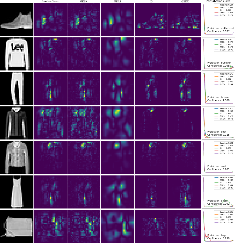
Figure S2: Sample explanations for the CNN trained on Fashion MNIST from different explanation methods, the last column presents the perturbation curves following explanations from the competitors until all pixels are masked out. Texts in the bottom half of the plots refer to the prediction on the original input.

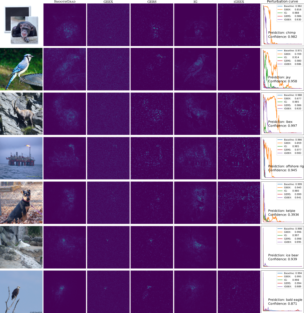
Figure S3: Sample explanations for Inception V3 pre-trained on ImageNet from different explanation methods, the last column presents the perturbation curves following explanations from the competitors until all pixels are masked out. Texts in the bottom half of the plots refer to the prediction on the original input.

S-V Effect of Hyperparameters

(a)

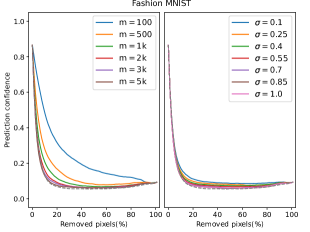
(b)

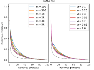
(c)

Figure S4: Effects of $m$ and $\sigma$ reported on (a) MNIST, (b) Fashion MNIST, and (c) ImageNet. For each group of charts, the left plot refers to the changes of perturbation curves while increasing the sample set size $m$ with $\sigma$ fixed to 1.0, the right plot presents the impact of changing the search range $\sigma$ with $m$ fixed to 5k. The dashed line indicates the baseline (SmoothGrad).

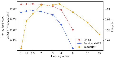
Figure S5: Trends of AOPC scores with varying $r$. The x-axis is on a logarithmic scale. Please note the different scales of the y-axis for MNIST / Fashion MNIST and ImageNet.

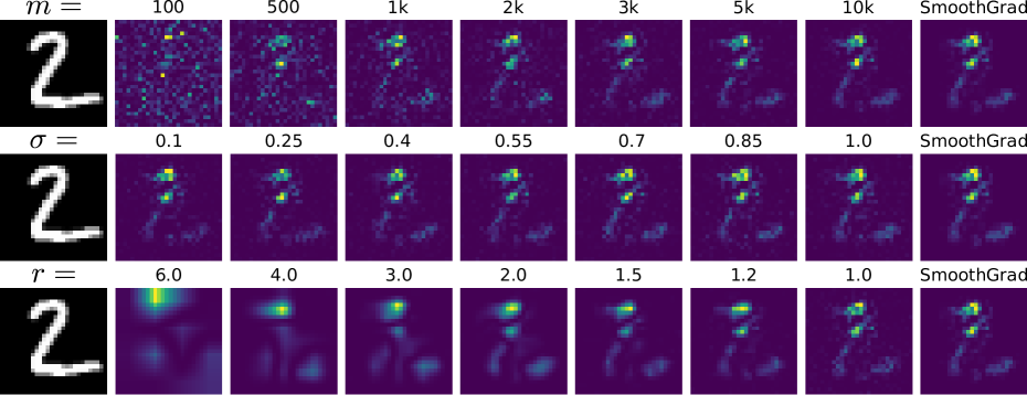
Figure S6: Explanations for the same decision under various hyperparameter settings

We study the effects of the three hyperparameters utilized by GEEX, namely the number of samples $m$, the search range $\sigma$, and the resizing ratio $r=\frac{h}{\hat{h}}$, to guide the selection of these values. We repeat the same experiment in all three test scenarios. The charts in Fig. S4 are grouped by the test scenarios. For each group, the plot on the right demonstrates the change of explanation quality when altering the sample set size $m$, whereas the left shows the impact of the search range $\sigma$. The dashed line represents the perturbation curve of the baseline as a reference. Aligning with the expectation, the number of samples $m$ positively correlates to the AOPC score in all scenarios. With the expanding sample set, the perturbation curves of GEEX converge to the gradient-based approach. For the MNIST and Fashion MNIST, the growing trend (of areas above a perturbation curve) slows down when the sample set reaches a certain size, which is 2k for both cases. By contrast, albeit relatively slowly, enlarging the sample set improves explanation quality constantly on ImageNet, indicating that the expanded feature space requests more samples for reliable estimations.

Surprisingly, the explanation quality seems more sensitive to sample set size $m$ in the simpler test scenarios than in the one (ImageNet) with a much larger input size. One cause of the difference in sensitivity is the distinct pixel value distributions. For MNIST and Fashion MNIST, most pixels have a value close to either pole of the domain, meaning they take the value of 0 or 255. Given that the default value for replacement is 0, any unfaithful explanations that mistakenly point to inactive regions would fall far behind due to the wasted moves. In addition, we find that the outcomes of the pre-trained Inception V3 model on ImageNet are susceptible to the deletion process. Deletion following a random order (simulating that no information is provided by explanations) attains a normalized AOPC score of 0.8381. The curve by random deletion reflects the lower bound of the deletion process, which is close to the upper bound of GEEX drawn by the baseline (0.9463). Consequently, the tight space between the bounds limits the possible change of the curves, meaning that the dependency of explanation quality on $m$ is under-represented by the comparison of curves.

The choice of $\sigma$ affects the explanation quality similarly. A more extensive search range exposes the gradients for flattened segments of a classification function, which subtly improves explanation quality. Besides, although not shown in the charts, we want to note that the value of $\sigma$ should be bounded. Otherwise, the derived sample $z=x+\sigma\epsilon$ is more likely to exceed the input domain, which could drag the focus of explanations away from the target data manifold.

The resizing ratio $r$ determines the trade-off between the preciseness and smoothness of derived explanations. Since the perturbation curves under varying $r$ overlap with each other, for better visibility, we summarize them with normalized AOPC scores and report the changing tendency in Fig. S5. In the case of the InceptionV3 model pre-trained on ImageNet, the performance of GERS peaks at $r=3.75$, which is the resizing ratio adopted during the quantitative evaluation, i.e. $\hat{h}=80$. Its explanations lose either preciseness or smoothness while heading towards the two extremes of the ratio, which causes the fall of the AOPC score. The sharper drop when reducing resizing ratio indicates that explanation quality in this scenario is more sensitive to noises. The peaks shift to the direction of lowering $r$ for the explanations on small inputs as a result of the undermined demand of denoising. Fig. S6 gives concrete examples regarding the impact of parameter selection on final explanations.

References

- [Bach et al. 2015] Bach, S.; Binder, A.; Montavon, G.; Klauschen, F.; Müller, K.-R.; and Samek, W. 2015. On pixel-wise explanations for non-linear classifier decisions by layer-wise relevance propagation. PloS one 10(7):e0130140.
- [Balduzzi et al. 2017] Balduzzi, D.; Frean, M.; Leary, L.; Lewis, J.; Ma, K. W.-D.; and McWilliams, B. 2017. The shattered gradients problem: If resnets are the answer, then what is the question? In International Conference on Machine Learning, 342–350. PMLR.
- [Brockhoff et al. 2010] Brockhoff, D.; Auger, A.; Hansen, N.; Arnold, D. V.; and Hohm, T. 2010. Mirrored sampling and sequential selection for evolution strategies. In Parallel Problem Solving from Nature, PPSN XI: 11th International Conference, Kraków, Poland, September 11-15, 2010, Proceedings, Part I 11, 11–21. Springer.
- [Fidel, Bitton, and Shabtai 2020] Fidel, G.; Bitton, R.; and Shabtai, A. 2020. When explainability meets adversarial learning: Detecting adversarial examples using shap signatures. In 2020 international joint conference on neural networks (IJCNN), 1–8. IEEE.
- [Friedman 2004] Friedman, E. J. 2004. Paths and consistency in additive cost sharing. International Journal of Game Theory 32:501–518.
- [Geirhos et al. 2020] Geirhos, R.; Jacobsen, J.-H.; Michaelis, C.; Zemel, R.; Brendel, W.; Bethge, M.; and Wichmann, F. A. 2020. Shortcut learning in deep neural networks. Nature Machine Intelligence 2(11):665–673.
- [Johnson 1911] Johnson, H. M. 1911. Clever hans (the horse of mr. von osten): A contribution to experimental, animal, and human psychology. The Journal of Philosophy, Psychology and Scientific Methods 8(24):663–666.
- [Lapuschkin et al. 2019] Lapuschkin, S.; Wäldchen, S.; Binder, A.; Montavon, G.; Samek, W.; and Müller, K.-R. 2019. Unmasking clever hans predictors and assessing what machines really learn. Nature communications 10(1):1096.
- [LeCun et al. 1998] LeCun, Y.; Bottou, L.; Bengio, Y.; and Haffner, P. 1998. Gradient-based learning applied to document recognition. Proceedings of the IEEE 86(11):2278–2324.
- [Mohseni, Block, and Ragan 2021] Mohseni, S.; Block, J. E.; and Ragan, E. 2021. Quantitative evaluation of machine learning explanations: A human-grounded benchmark. In 26th International Conference on Intelligent User Interfaces, 22–31.
- [Montavon et al. 2017] Montavon, G.; Lapuschkin, S.; Binder, A.; Samek, W.; and Müller, K.-R. 2017. Explaining nonlinear classification decisions with deep taylor decomposition. Pattern recognition 65:211–222.
- [Petsiuk, Das, and Saenko 2018] Petsiuk, V.; Das, A.; and Saenko, K. 2018. Rise: Randomized input sampling for explanation of black-box models. In Proceeedings of the British Machine Vision Conference 2018, BMVC 2018, Newcastle, UK.
- [Ribeiro, Singh, and Guestrin 2016] Ribeiro, M. T.; Singh, S.; and Guestrin, C. 2016. “why should i trust you?” explaining the predictions of any classifier. In Proceedings of the 22nd ACM SIGKDD international conference on knowledge discovery and data mining, 1135–1144.
- [Russakovsky et al. 2015] Russakovsky, O.; Deng, J.; Su, H.; Krause, J.; Satheesh, S.; Ma, S.; Huang, Z.; Karpathy, A.; Khosla, A.; Bernstein, M.; et al. 2015. Imagenet large scale visual recognition challenge. International journal of computer vision 115:211–252.
- [Russell 2010] Russell, S. J. 2010. Artificial intelligence a modern approach. Pearson Education, Inc.
- [Salimans et al. 2017] Salimans, T.; Ho, J.; Chen, X.; Sidor, S.; and Sutskever, I. 2017. Evolution strategies as a scalable alternative to reinforcement learning. arXiv preprint arXiv:1703.03864.
- [Samek et al. 2016] Samek, W.; Binder, A.; Montavon, G.; Lapuschkin, S.; and Müller, K.-R. 2016. Evaluating the visualization of what a deep neural network has learned. IEEE transactions on neural networks and learning systems 28(11):2660–2673.
- [Shrikumar et al. 2016] Shrikumar, A.; Greenside, P.; Shcherbina, A.; and Kundaje, A. 2016. Not just a black box: Learning important features through propagating activation differences. arXiv preprint arXiv:1605.01713.
- [Simonyan, Vedaldi, and Zisserman 2014] Simonyan, K.; Vedaldi, A.; and Zisserman, A. 2014. Deep inside convolutional networks: visualising image classification models and saliency maps. In Proceedings of the International Conference on Learning Representations. ICLR.
- [Smilkov et al. 2017] Smilkov, D.; Thorat, N.; Kim, B.; Viégas, F.; and Wattenberg, M. 2017. Smoothgrad: removing noise by adding noise. In Proceedings of the ICML Workshop on Visualization for Deep Learning, Sydney, Australia, 10 August 2017.
- [Sundararajan, Taly, and Yan 2017] Sundararajan, M.; Taly, A.; and Yan, Q. 2017. Axiomatic attribution for deep networks. In International conference on machine learning, 3319–3328. PMLR.
- [Szegedy et al. 2015] Szegedy, C.; Liu, W.; Jia, Y.; Sermanet, P.; Reed, S.; Anguelov, D.; Erhan, D.; Vanhoucke, V.; and Rabinovich, A. 2015. Going deeper with convolutions. In Proceedings of the IEEE conference on computer vision and pattern recognition, 1–9.
- [Szegedy et al. 2016] Szegedy, C.; Vanhoucke, V.; Ioffe, S.; Shlens, J.; and Wojna, Z. 2016. Rethinking the inception architecture for computer vision. In Proceedings of the IEEE conference on computer vision and pattern recognition, 2818–2826.
- [Vedaldi and Soatto 2008] Vedaldi, A., and Soatto, S. 2008. Quick shift and kernel methods for mode seeking. In Computer Vision–ECCV 2008: 10th European Conference on Computer Vision, Marseille, France, October 12-18, 2008, Proceedings, Part IV 10, 705–718. Springer.
- [Watson and Al Moubayed 2021] Watson, M., and Al Moubayed, N. 2021. Attack-agnostic adversarial detection on medical data using explainable machine learning. In 2020 25th International Conference on Pattern Recognition (ICPR), 8180–8187. IEEE.
- [Wierstra et al. 2014] Wierstra, D.; Schaul, T.; Glasmachers, T.; Sun, Y.; Peters, J.; and Schmidhuber, J. 2014. Natural evolution strategies. The Journal of Machine Learning Research 15(1):949–980.
- [Xiao, Rasul, and Vollgraf 2017] Xiao, H.; Rasul, K.; and Vollgraf, R. 2017. Fashion-mnist: a novel image dataset for benchmarking machine learning algorithms. arXiv preprint arXiv:1708.07747.
- [Zeiler and Fergus 2014] Zeiler, M. D., and Fergus, R. 2014. Visualizing and understanding convolutional networks. In Computer Vision–ECCV 2014: 13th European Conference, Zurich, Switzerland, September 6-12, 2014, Proceedings, Part I 13, 818–833. Springer.
Supplementary Material