CARLA: Self-supervised Contrastive Representation Learning for Time Series Anomaly Detection

Abstract

One main challenge in time series anomaly detection (TAD) is the lack of labelled data in many real-life scenarios. Most of the existing anomaly detection methods focus on learning the normal behaviour of unlabelled time series in an unsupervised manner. The normal boundary is often defined tightly, resulting in slight deviations being classified as anomalies, consequently leading to a high false positive rate and a limited ability to generalise normal patterns. To address this, we introduce a novel end-to-end self-supervised ContrAstive Representation Learning approach for time series Anomaly detection (CARLA). While existing contrastive learning methods assume that augmented time series windows are positive samples and temporally distant windows are negative samples, we argue that these assumptions have limitations as augmentation of time series can transform them to negative samples, and a temporally distant window can represent a positive sample. Our contrastive approach leverages existing generic knowledge about time series anomalies and injects various types of anomalies as negative samples. Therefore, CARLA not only learns normal behaviour but also learns deviations indicating anomalies. It creates similar representations for temporally closed windows and distinct ones for anomalies. Additionally, it leverages the information about representations’ neighbours through a self-supervised approach to classify windows based on their nearest/furthest neighbours in the representation space to further enhance the performance of anomaly detection. In extensive experiments on seven large real-world time series anomaly detection datasets, CARLA shows superior performance (F1 and AU-PR) over state-of-the-art self-supervised and unsupervised TAD methods for univariate and multivariate series. Our research highlights the immense potential of contrastive representation learning in advancing the time series anomaly detection field, thus paving the way for novel applications and in-depth exploration in the domain.

I Introduction

Detecting anomalies is crucial in a range of fields, such as finance, healthcare, and cybersecurity. In time series data, anomalies can result from different factors, including equipment failure, sensor malfunction, human error, and human intervention. Detecting anomalies in time series data has numerous real-world uses, including monitoring equipment for malfunctions, detecting unusual patterns in IoT sensor data, enhancing the reliability of computer programs and cloud systems, observing patients’ health metrics, and pinpointing cyber threats. Time series anomaly detection (TAD) has been the subject of decades of intensive research, with numerous approaches proposed to address the challenge of spotting rare and unexpected events in complex and noisy data. Statistical methods have been developed to monitor and identify abnormal behaviour [1, 2, 3]. Recent advancements in deep learning techniques have effectively tackled various anomaly detection problems [4]. Specifically, for time series with complex nonlinear temporal dynamics, deep learning methods have demonstrated remarkable performance [5].

Most of these models focus on learning the normal behaviour of data from an unlabelled dataset, and therefore have the ability to predict samples that deviate from the normal behaviour as anomalies. The lack of labelled data in real-world scenarios makes it difficult for models to learn the difference between normal and anomalous behaviours. The normal boundary is often tightly defined, which can result in slight deviations being classified as anomalies. Models that cannot discriminate between normal and anomaly classes may predict normal samples as anomalous, leading to a high false positive rate of detection as demonstrated in Fig. 1-a. It shows a histogram of anomaly detection scores of an existing TAD called THOC [6] on a benchmark test dataset. Many normal data are assigned high anomaly scores leading to false positives.

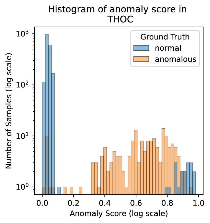
(a)

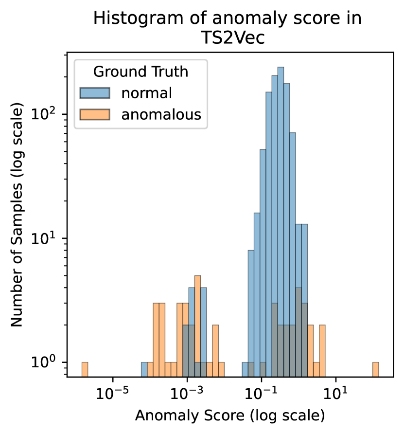
(b)

Figure 1: Histogram of anomaly scores produced by (a) THOC model [6] and (b) TS2Vec model [7]. Histograms illustrating the distribution of anomaly scores for the THOC and TS2Vec models using data from entity M-6 of the MSL dataset [8].

An alternative approach is to leverage the power of self-supervised contrastive representation learning. Contrastive learning entails training a model to differentiate between pairs of similar and dissimilar samples in a dataset. Contrastive representation learning has been successful in image [9] and text data [10], and its potential and effectiveness in TAD are being explored in the recent years. However, existing contrastive learning methods for TAD assume that augmented time series windows are positive samples and temporally distant windows are negative samples. We argue that these assumptions carry the risk that augmentation of time series can transform them to negative samples, and a temporally distant window can represent a positive sample leading to ineffective AD performance. Fig. 1-b shows anomaly scores of a contarstive learning method called TS2Vec [7]. As demonstrated, the anomaly scores of both normal and anomalous data are intermingled, resulting in the inefficacy of anomaly detection.

We propose a novel two-stage framework called CARLA, designed specifically to enhance time series anomaly detection. Our novel approach addresses the lack of labelled data through a contrastive approach which leverages existing generic knowledge about time series anomalies. We inject various types of anomalies, which facilitates the learning representations of normal behaviour. This is achieved by encouraging the learning of similar representations for windows that are temporally closed windows, while ensuring dissimilar representations for windows and their corresponding injected anomalous windows.

Additionally, to ensure that the representation of exisiting real anomalous windows are different from normal representations we employ a self-supervised approach to classify normal/anomalous representations of windows based on their nearest/furthest neighbours in the representation space. By making the normal representations more discriminative, we enhance the anomaly detection performance in our proposed model. Specifically, the main contributions of this paper can be summarised as follows:

• We propose a novel contrastive representation learning model to detect anomalies in time series, which delivers top-tier outcomes across a range of benchmark datasets, encompassing both univariate time series and multivariate time series. This model utilises a self-supervised approach to learn normal samples which are effectively discriminative from anomalous samples’ in the feature representation space.

• We propose an effective contrastive method for TAD to learn feature representations for a pretext task by leveraging existing generic knowledge about time series anomalies (see Fig. 4(a)).

• We propose a self-supervised method that leverages the representations learned in the pretext stage to classify time series windows. We aim to classify each sample by utilising its neighbours in the representation space which were learned during the pretext stage (see Fig. 4).

• Our extensive evaluation on 7 real-world benchmark datasets and the metrics employed demonstrate the robustness and effectiveness of CARLA, thereby highlighting the substantial contribution of our work.

II Related Works

In this section, we provide a brief survey of the existing literature that intersects with our research. We concentrate on three areas: deep learning for anomaly detection in time series, unsupervised representation of time series, and the contrasting representation learning technique.

II-A Time Series Anomaly Detection

The detection of anomalies within time series data has been the subject of extensive research, using an array of techniques from statistical methods to classical machine learning and, more recently, deep learning models [11, 12]. Established statistical techniques such as moving averages, exponential smoothing [13], and the ARIMA model [14] have seen the widespread application. Machine learning techniques, including clustering algorithms such as k-means [15] and density-based approaches, alongside classification algorithms like decision trees [16, 17] and SVMs, have also been leveraged.

Deep Learning methods in TAD: In recent years, deep learning models have demonstrated potential in addressing the complexities of TAD due to their capacity to autonomously extract features from raw data [5]. Prior research has leaned toward unsupervised [7, 8, 18, 19, 20] or semi-supervised [21, 22, 23, 24] techniques due to the paucity of labelled data in real-world scenarios [5]. The preference for models like LSTM-AD [25], LSTM-NDT [8], DITAN [26] and THOC [6] is because they excel at minimising forecasting errors while capturing time series data’s temporal dependencies.

Anomaly detection within time series data has also benefitted from autoencoder-based deep models like DAGMM [27], USAD [18], MSCRED [28], DAEMON [29] and the recent work by [30]. These models primarily exploit the reconstruction error to compute an anomaly score. However, a common limitation with these models is the accumulation of errors when decoding extensive sequences, leading to a subpar performance on long time series. Although recurrent variational autoencoders [31] have been proposed as robust alternatives, they are still restricted by the presumption that the data adheres to a specific distribution, typically Gaussian. This may not be the case for all types of data and can result in less than optimal performance.

GANs and their variants such as MAD-GAN [32] and BeatGAN [33] have also been explored for TAD. However, these models pose training challenges, with preventing mode collapse being a pivotal concern that demands a balance between the discriminator and generator [34].

Deep learning techniques, encompassing autoencoders, VAEs [24, 35], RNNs [36, 31], and LSTM networks [8, 23, 25], have shown potential in spotting anomalies within time series, particularly for high-dimensional or non-linear data.

In sum, deep learning has heralded the development of two distinct types of time series anomaly detection algorithms: supervised and unsupervised [37]. Semi-supervised methods, such as AutoEncoder [35], LSTM-VAE [24] excel when labels are readily available. On the other hand, unsupervised methods, such as OmniAnomaly [31], DAGMM [27], GDN [38], and RDSSM [39], become more suitable when obtaining anomaly labels is a challenge. These unsupervised deep learning methods are preferred due to their capability to learn robust representations without requiring labelled data. Most of these methods follow a reconstruction-based approach, where the model is trained to reconstruct normal data, and instances that fail to be accurately reconstructed are marked as anomalies. The advent of self-supervised learning-based methods has further improved generalization ability in unsupervised anomaly detection [40, 41, 42].

II-B Unsupervised Time Series Representation

The demonstration of substantial performance by unsupervised representation learning across a wide range of fields, such as computer vision [9, 43, 44, 45], natural language processing [46, 47], and speech recognition [48, 49], has made it a desirable technique. In the realm of time series, methods like SPIRAL [50], TimeNet [51], RWS [52], TKAE [53] and TST [54] have been suggested. While these methods have made significant contributions, some of them face challenges with scalability for exceptionally long time series or encounter difficulties in modelling complex time series. To overcome these limitations, methods such as TNC [55] and T-Loss [56] have been proposed advancing the use of triplet loss. They leverage time-based negative sampling, triplet loss, and local smoothness of signals for the purpose of learning multivariate time series representations that are scalable. Triplet loss initially pioneered by RAMODO [57], significantly enhances outlier detection capabilities. TSTCC [58] emphasizes consistency among different data augmentations. Despite their merits, these methods often limit their universality by learning representations particular semantic tier, relying on significant assumptions regarding invariance during transformations.

II-C Contrastive Representation Learning

Contrastive representation learning creates an embedding space where similar samples are close, and dissimilar ones are distant, applicable in domains like natural language processing, computer vision, and time series anomaly detection [59]. Traditional models like InfoNCE loss [60], SwAV [61], SimCLR [9], and MoCo [62] use positive-negative pairs to optimize this space, demonstrating strong performance and paving the way for advanced techniques.

Siamese architectures such as BYOL [63] and SimSiam [64] represent a significant advancement by eliminating the need for negative samples, focusing solely on positive pairs. These models simplify the architecture while maintaining competitive performance.

In time series anomaly detection, contrastive learning is crucial for recognizing patterns. TS2Vec [7] uses this approach hierarchically for multi-level semantic representation, while DCdetector [37] introduces a dual attention asymmetric design with pure contrastive loss, enabling permutation invariant representations.

III CARLA

Problem definition: Given a time series $\mathcal{D}$ which is partitioned into $m$ overlapping time series windows $\{w_{1},..,w_{i},..,w_{m}\}$ with stride 1 where $w_{i}=\{x_{1},..,x_{i},..,x_{WS}\}$, $WS$ is time series window size, $x_{i}\in\mathbb{R}^{Dim}$ and $Dim$ is the dimension of time series, the goal is to detect anomalies in time series windows.

CARLA (A Self-supervised ContrAstive Representation Learning Approach for time series Anomaly detection) is built on several key components, each of which plays a critical role in achieving effective representation learning as illustrated in Fig. 2. CARLA consists of two main stages: the Pretext Stage and the Self-supervised Classification Stage.

Initially, in the Pretext Stage (section III-B), it employs anomaly injection to learn similar representations for temporally proximate windows and distinct representations for windows and their equivalent anomalous windows (section III-A). These injected anomalies include point anomalies, such as sudden spikes, and subsequence anomalies, like unexpected pattern shifts. This technique not only aids in training the model to recognise deviations from the norm but also strengthens its ability to generalise across various types of anomalies. At the end of the Pretext Stage, we establish a prior by finding the nearest and furthest neighbours for each window representation for the next stage. The Self-supervised Classification Stage (section III-C) then classifies these window representations as normal or anomalous based on the proximity of their neighbours in the representation space (section III-D). This classification aims to group similar time series windows together while distinctly separating them from dissimilar ones. The effectiveness of this stage is pivotal in accurately categorising time series windows, reinforcing CARLA’s capability to differentiate between normal and anomalous patterns. The comprehensive end-to-end pipeline of CARLA, including these stages, is illustrated in Fig. 2.

The following sections present the cornerstones of our approach.

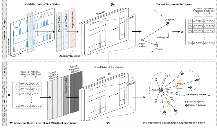
Figure 2: The end-to-end pipeline of CARLA consists of two main stages: the Pretext Stage and the Self-supervised Classification Stage. In the Pretext Stage, anomaly injection techniques are used for self-supervised learning. The Self-supervised Classification Stage integrates the learned representations for a contrastive approach that maximizes the similarity between anchor samples and their nearest neighbours while minimising the similarity between anchor samples and their furthest neighbours. The output is a trained model and the majority class, enabling inference for anomaly detection.

III-A Anomaly Injection

The technique of anomaly injection, a potent data augmentation strategy for time series, facilitates the application of self-supervised learning in the absence of ground-truth labels. While the augmentation methods we employ are not designed to represent every conceivable anomaly type [65]—a goal that would be unattainable— they amalgamate various robust and generic heuristics to effectively identify prevalent out-of-distribution instances.

III-A1 Anomaly Injection Steps

During the training phase, each window is manipulated by randomly choosing instances within a given window $w_{i}$. Two primary categories of anomaly injection models—point anomalies and subsequence anomaly—are adopted to inject anomalies to a time series window $w_{i}$. In a multivariate time series context, a random start time and a subset of dimension(s) $d$ are selected for the injection of a point or subsequence anomalies. Note in the context of multivariate time series, anomalies are not always present across all dimensions, prompting us to randomly select a subset of dimensions for the induced anomalies ($d<\lceil Dim/10\rceil$). The injected anomaly portion for each dimension varied from 1 data point to 90% of the window length.

This approach fosters the creation of a more diverse set of anomalies, enhancing our model’s capability of detecting anomalies exist in multiple dimensions. This approach strengthen our model’s effectiveness in discriminating normal and anomalous representations in the Pretext Stage. It is important to underscore that the anomaly injection strategies employed in our model’s evaluation were consistently applied across all benchmarks to ensure a fair and impartial comparison of the model’s performance across various datasets. The detailed step-by-step process for our anomaly injection approach is elaborated in Algorithm 1. This comprehensive algorithm encapsulates the methodology of both point anomaly injection and subsequence anomaly injection, providing a clear understanding of our process and its implementation.

Algorithm 1 InjectAnomaly($w$)

1:Time series window $w$

2:Anomaly injected time series window $w$

3:$types\leftarrow\{\texttt{Seasonal},\texttt{Trend},\texttt{Global},\texttt{Contextual},\texttt{Shapelet}\}$

4:$Dim\leftarrow\text{random subset of dimensions of }w~{}\text{(for UTS, }Dim=\{1\}\text{)}$

5:$s,e\leftarrow\text{random start and end points from }(0,size(w))\text{, where }e>s$

6:for each dimension $d$ in $Dim$ do

7:    $anomlaly\leftarrow\text{randomly choose anomaly type from }types$

8:    if $anomaly=\texttt{Global }or\texttt{ Contextual}$ then

9:        $t=(s+e)/2$ $\triangleright$ random point in $w$

10:        Inject the $anomaly$ at time point $t$ in dimensions $d$

11:    else if $anomaly=\texttt{Seasonal }or\texttt{ Trend }or\texttt{ Shapelet}$ then

12:        $W\leftarrow(W^{(s)},\ W^{(e)})$ $\triangleright$ subsequence of $w$

13:        Inject the $anomaly$ in $W$ in dimensions $d$

14:    end if

15:end for

16:Return $w$

III-A2 Point Anomalies

Our methodology incorporates the injection of single point anomalies (a spike) at randomly chosen instances within a given window $w_{i}$. In a multivariate time series context, a randomly selected subset of dimensions $d$ (where $d<\lceil Dim/10\rceil$) is selected for the injection of a point anomaly/spike. Serving as distinctly labelled abnormal points, these point anomalies aid in creating a model of the normal representation. We employ two distinct types of point anomalies, namely, Global (Fig. 3(b)) and Contextual (Fig. 3(c)).

(a)

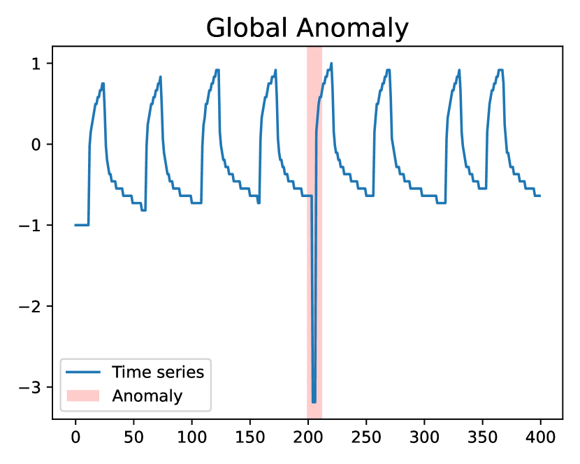
(b)

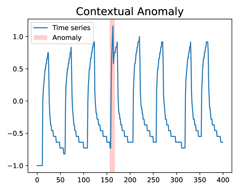
(c)

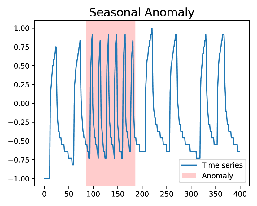
(d)

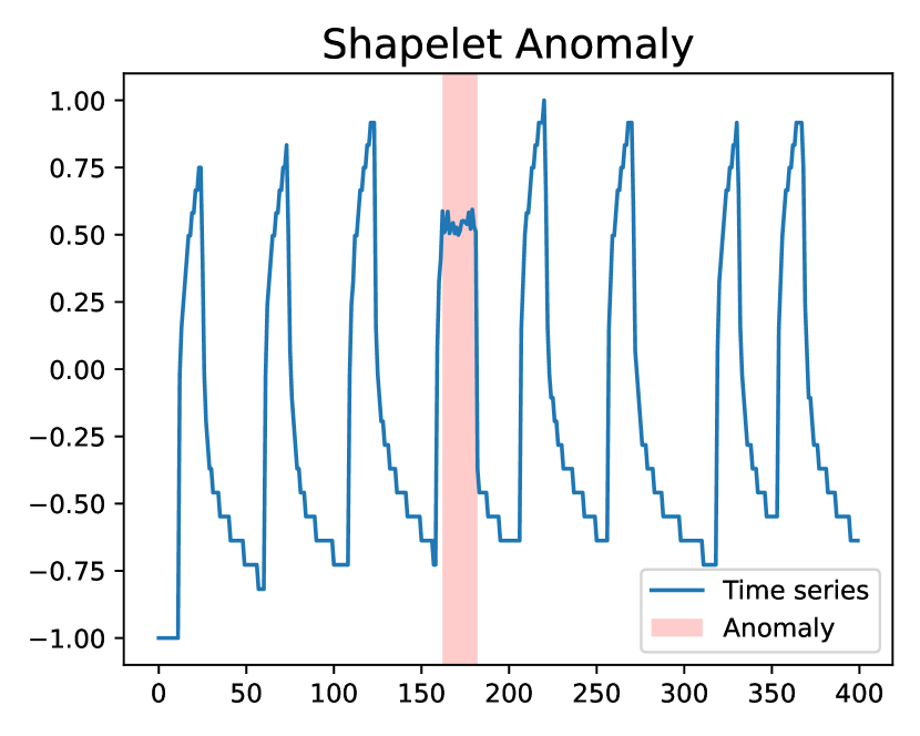
(e)

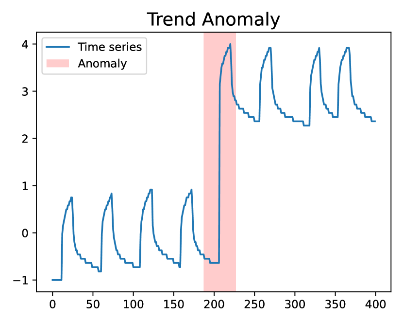
(f)

Figure 3: Different types of synthetic anomaly injection used in CARLA. (a) represents the original time series window from entity E-2 in the MSL dataset [8]. The anomalies are categorised as (b) Global, (c) Contextual, (d) Seasonal, (e) Shapelet, and (f) Trend.In all five plots, the anomalous points or subsequences are accentuated with a red colour.

III-A3 Subsequence Anomalies

The technique of subsequence anomaly injection, motivated by the successful implementation of the Outlier Exposure approach [66], enhances anomaly detection in time series data by generating contextual out-of-distribution examples. It involves the introduction of a subsequence anomaly within a time series window $w_{i}$, represented as $W_{i}=(W_{i}^{(s)},\ W_{i}^{(e)})$, where $W_{i}^{(s)}$ denotes the anomaly’s starting time point and $W_{i}^{(e)}$ represents its endpoint. We explore three primary types of subsequence (aka pattern) anomalies: Seasonal (Fig. 3(a)), Shapelet (Fig. 3(e)), and Trend (Fig. 3(f)).

III-B Pretext Stage

The Pretext Stage of CARLA consists of two parts: Part One is a contrastive representation learning step that uses a ResNet architecture (which has shown effectiveness in times series classification tasks [67]) to learn representations for time series windows, and Part Two is a post-processing step that uses the learned representations from Part One to identify semantically meaningful nearest and furthest neighbours for each learned window representation. Algorithm 2 shows the Pretext steps.

Algorithm 2 PretextCARLA($\mathcal{D}$, $Q$, $\alpha$)

1:Sequential time series windows $\mathcal{D}=\{w_{1},w_{2},...,w_{m}\}$, number of nearest/furthest neighbours $Q$, margin $\alpha$.

2:Trained model $\phi_{p}$, all neighbours set $\mathcal{B}$, nearest neighbours set $\mathcal{N}$, furthest neighbours set $\mathcal{F}$.

3:$\mathcal{T}\leftarrow\varnothing$, $\mathcal{B}\leftarrow\varnothing$, $\mathcal{N}\leftarrow\varnothing$, $\mathcal{F}\leftarrow\varnothing$

4:for $i\leftarrow 1$ to $|\mathcal{D}|$ do

5:    $a_{i}\leftarrow w_{i}$ $\triangleright$ anchor

6:    $p_{i}\leftarrow w_{i-r}$, where $r\sim\mathcal{U}(1,y)$ $\triangleright$ positive pair

7:    $n_{i}\leftarrow$ InjectAnomaly($w_{i}$) $\triangleright$ negative pair (Alg. 1)

8:    append triplet $(a_{i},p_{i},n_{i})$ to $\mathcal{T}$ $\triangleright$ triplets batches

9:    add $a_{i}$ and $n_{i}$ to $\mathcal{B}$ $\triangleright$ neighbours set with size $2|\mathcal{D}|$

10:end for

11:while Pretext loss $\mathcal{L}_{pretext}(\phi_{p},\mathcal{T},\alpha)$ decreases do

12:    Update $\phi_{p}$ with $\mathcal{L}_{pretext}$ $\triangleright$ i.e. Equation (1)

13:end while

14:for $j\leftarrow 1$ to $|\mathcal{B}|$ do

15:    $\mathcal{N}_{j}\leftarrow Q$ nearest neighbours of $w_{j}\in\mathcal{B}$ in $\phi_{p}(\mathcal{B})$ space

16:    $\mathcal{F}_{j}\leftarrow Q$ furthest neighbours of $w_{j}\in\mathcal{B}$ in $\phi_{p}(\mathcal{B})$ space

17:end for

18:Return $\phi_{p}$, $\mathcal{B}$, $\mathcal{N}$, $\mathcal{F}$ $\triangleright$ inputs of the next stage

III-B1 Part One: Contrastive Representation Learning

In this part, we intorduce a contrastive learning framework for learning a discriminative representation of features for time series windows. To extract features from the time series data, we utilise a multi-channel ResNet architecture, where each channel represents a different time series dimension. Using different kernel sizes in ResNet allows us to capture features at various temporal scales, which is particularly important in analysing time series data and makes our model less sensitive to window size selection. We add an MLP layer as the final layer to produce a feature vector with lower dimensions.

To encourage the model to distinguish between different time series windows, we utilise a triplet loss function. Specifically, we create triplets of samples in the form of $(a,p,n)$, where $a$ is the anchor sample (i.e. the original time series window $w_{i}$), $p$ is a positive sample (i.e. another random window selected from $y$ previous windows $w_{i-r}$, where $r\sim\mathcal{U}(1,y)$), and $n$ is a negative sample (i.e. an anomaly injected version of the original window to make it anomalous). Assuming we have all the triplets of $(a,p,n)$ in a set $\mathcal{T}$, the pretext triplet loss function is defined as follows:

$$\mathcal{L}_{Pretext}(\phi_{p},\mathcal{T},\alpha)=$$ (1)

$$\frac{1}{|\mathcal{T}|}\sum_{(a,p,n)\in\mathcal{T}}\max(\lVert\phi_{p}(a)-\phi_{p}(p)\rVert_{2}^{2}-\lVert\phi_{p}(a)-\phi_{p}(n)\rVert_{2}^{2}+\alpha,0)$$

where $\phi_{p}(\cdot)$ is the learned feature representation neural network, $\lVert\cdot\rVert_{2}^{2}$ denotes the squared Euclidean distance, and $\alpha$ is a margin that controls the minimum distance between positive and negative samples. The objective of the pretext triplet loss function is to decrease the distance between the anchor sample and its corresponding positive sample while simultaneously increasing the distance between the anchor sample and negative samples. This approach encourages the model to learn a representation that can differentiate between normal and anomalous time series windows.

Our approach empowers the model to learn similar feature representations for temporally proximate windows. Since in anomaly detection datasets the majority of data is normal, the model captures temporal relationships of normal data through learning similar representations for normal windows that are temporally proximate. Furthermore, by introducing anomalies into the system, the model can learn a more effective decision boundary, resulting in a reduced false positive rate and enhanced precision in identifying anomalies when compared to current state-of-the-art models.

The output of Part One includes a trained neural network (ResNet) $\phi_{p}$ and a list of anchor and negative samples stored in $\mathcal{B}$.

III-B2 Part Two: Nearest and Furthest Neighbours

Part Two of our approach uses the feature representations learned in Part One to identify semantically meaningful nearest and furthest neighbours for each sample. To achieve this, we utilise $\mathcal{B}$ along with the indices of $Q$ nearest and $Q$ furthest neighbours of all samples in $\mathcal{B}$.

The primary goal of this part is to generate a prior that captures the semantic similarity and semantic dissimilarity between windows’ representations using their neighbours, as our empirical analysis shows that in the majority of cases, these nearest neighbours belong to the same class (see Fig. 4(a)). Semantic similarity for a given window $w_{i}$ defines as $Q$ nearest neighbours of $\phi_{p}(w_{i})\in\phi_{p}(\mathcal{B})$, where $Q$ is the number of nearest neighbours. And, semantic dissimilarity for a given window $w_{i}$ defined as $Q$ furthest neighbours of $\phi_{p}(w_{i})\in\phi_{p}(\mathcal{B})$. The output of Part Two is a set of all anchor and negative samples (anomaly injected) and the indices of their $Q$ nearest neighbours $\mathcal{N}$ and $Q$ furthest neighbours $\mathcal{F}$. Utilising $\mathcal{N}$ and $\mathcal{F}$ can enhance the performance of our classification method used in the Self-supervised Classification Stage.

III-C Self-supervised Classification Stage

This stage includes initialising a new ResNet architecture with the learned feature representations from Part One of the Pretext Stage and then integrating the semantically meaningful nearest and furthest neighbours from Part Two as a prior ($\mathcal{N}$ and $\mathcal{F}$) into a learnable approach. Algorithm 3 shows the steps of the Self-supervised classification Stage.

Algorithm 3 SelfSupevisedCARLA($\phi_{p}$, $\mathcal{B}$, $\mathcal{N}$, $\mathcal{F}$, $C$, $\beta$)

1:Initial trained neural network (ResNet) from the Pretext Stage $\phi_{p}$, Dataset of time series windows including original windows and anomaly injected windows $\mathcal{B}$, Set of $Q$ nearest neighbours for each window $\mathcal{N}$, Set of $Q$ furthest neighbours for each window $\mathcal{F}$, Number of Classes $C$, Entropy loss weight $\beta$

2:Trained model $\phi_{s}$, Majority class $C_{m}$

3:$\phi_{s}\leftarrow$ initialise by $\phi_{p}$ $\triangleright$ $\phi_{p}$ from Algorithm 2 (PretextCARLA)

4:while $\mathcal{L}_{Self-supervised}(\phi_{s},\mathcal{B},\mathcal{N},\mathcal{F},\mathcal{C},\beta)$ decreases do

5:    Update $\phi_{s}$ with $\mathcal{L}_{Self-supervised}$ $\triangleright$ i.e. Equation (6)

6:end while

7:for $i\leftarrow 1$ to $|\mathcal{D}|$ do

8:    $C^{i}=\arg\max(\phi_{s}(w_{i})),w_{i}\in\mathcal{D}$ $\triangleright$ assign class label $C_{j}\in\mathcal{C}$ to window $i$

9:end for

10:$C_{m}=\arg\max_{C_{j}\in\mathcal{C}}(n(C_{j}))$ $\triangleright$ find majority class $C_{m}$ $\triangleright$ $n(C_{j})$ denotes the number of members in a class $C_{j}$

11:Return $\phi_{s}$, $C_{m}$

To encourage the model to produce both consistent and discriminative predictions, we employ a contrastive approach with a customised loss function. Specifically, the loss function maximises the similarity between each window representations and its nearest neighbours, while minimising the similarity between each window representations and its furthest neighbours. The loss function can be defined as follows: At the beginning of this stage, we have $\mathcal{B}$ from the Pretext Stage which is the set of all original window representations (we call them anchors in this stage) and their corresponding anomalous representations. Let $C$ be the number of classes. We also have the $Q$ nearest neighbours of the anchor samples $\mathcal{N}$, and the $Q$ furthest neighbours of the anchor samples $\mathcal{F}$.

We aim to learn a classification neural network function $\phi_{s}$ - initialised by $\phi_{p}$ from the Pretext Stage - that classifies a window $w_{i}$ and its $Q$ nearest neighbours to the same class, and $w_{i}$ and its $Q$ furthest neighbours to different classes. The neural network $\phi_{s}$ terminates in a softmax function to perform a soft assignment over the classes $\mathcal{C}=\{1,...,C\}$, with $\phi_{s}(w)\in[0,1]^{C}$.

To encourage similarity between the anchor samples and their nearest neighbours, we compute the pairwise similarity between the probability distributions of the anchor and its neighbours as it is shown in Equation (2). The dot product between an anchor and its neighbour will be maximal when the output of the softmax for them is close to 1 or 0, and consistent that assigns to the same class. Then we define a consistency loss in Equation (LABEL:eq:consistencyloss) using the binary cross entropy to maximise the similarity between the anchor and nearest neighbours.

$$\text{similarity}(\phi_{s},w_{i},w_{j})=\langle\phi_{s}(w_{i})\cdot\phi_{s}(w_{j})\rangle=\phi_{s}(w_{i})^{\top}\phi_{s}(w_{j})$$ (2)

$$\mathcal{L}_{consistency}(\phi_{s},\mathcal{B},\mathcal{N})=$$ (3)

$$-\frac{1}{\lvert\mathcal{B}\rvert}\sum_{w\in\mathcal{B}} \sum_{w_{n}\in\mathcal{N}_{w}}\log(\text{similarity}(\phi_{s},w,w_{n}))$$

We define an inconsistency loss to encourage dissimilarity between the anchor samples and their furthest neighbours in Equation (LABEL:eq:inconsistencyloss). In this regard, we compute the pairwise similarity between the probability distributions of the anchor and furthest neighbour samples as well. Then use the binary cross entropy loss to minimise the similarity to the furthest neighbours in the final loss function.

$$\mathcal{L}_{inconsistency}(\phi_{s},\mathcal{B},\mathcal{F})=$$ (4)

$$-\frac{1}{\lvert\mathcal{B}\rvert}\sum_{w\in\mathcal{B}} \sum_{w_{n}\in\mathcal{F}_{w}}\log(\text{similarity}(\phi_{s},w,w_{n}))$$

To encourage class diversity and prevent overfitting, we use entropy loss on the distribution of anchor and neighbour samples across classes. Assuming the classes set is denoted as $\mathcal{C}=\{1,...,C\}$, and the probability of window $w_{i}$ being assigned to class $c$ is denoted as $\phi_{s}^{c}(w_{i})$:

$$\begin{split}\mathcal{L}_{entropy}(\phi_{s},\mathcal{B},\mathcal{C})=\sum_{c\in\mathcal{C}}\hat{\phi_{s}^{c}}\log(\hat{\phi_{s}^{c}})\\ \text{ where }\hat{\phi_{s}^{c}}=\frac{1}{\lvert\mathcal{B}\rvert}\sum_{w_{i}\in\mathcal{B}}\phi_{s}^{c}(w_{i})\end{split}$$ (5)

The final objective in the Self-supervised Classification Stage is to minimise the total loss, calculated by the difference between the consistency and inconsistency losses, reduced by the entropy loss multiplied by a weight parameter, $\beta$:

$$\mathcal{L}_{Self-supervised}(\phi_{s},\mathcal{B},\mathcal{N},\mathcal{F},\mathcal{C},\beta)=$$ (6)

$$\mathcal{L}_{consistency}(\phi_{s},\mathcal{B},\mathcal{N})-$$

$$\mathcal{L}_{inconsistency}(\phi_{s},\mathcal{B},\mathcal{F})-$$

$$\beta\cdot\mathcal{L}_{entropy}(\phi_{s},\mathcal{B},\mathcal{C})$$

The goal of the loss function is to learn a representation that is highly discriminative, with nearest neighbours assigned to the same class as the anchor samples, and furthest neighbours assigned to a distinct class. By incorporating the semantically meaningful nearest and furthest neighbours, the model is able to produce more consistent and confident predictions, with the probability of a window being classified as one particular class being close to 1 or 0.

Overall, the loss function $\mathcal{L}_{Self-supervised}$ represents a critical component of our approach to time series anomaly detection, as it allows us to effectively learn a discriminative feature representation that can be utilised to distinguish between normal and anomalous windows.

III-D CARLA’s Inference

Upon completing Part Two of our approach, we determine the class assignments for set $\mathcal{D}$ and majority class $C_{m}$, where $C_{m}=\arg\max_{C_{j}\in\mathcal{C}}(n(C_{j}))$ which comprises the class with the highest number of anchors (i.e. original windows). For every new window $w_{t}$ during inference, we calculate $\phi_{s}^{C_{m}}(w_{t})$, representing the probability of window $w_{t}$ being assigned to the majority class $C_{m}$. Using an end-to-end approach, we classify a given window $w_{t}$ as normal or anomalous based on whether it belongs to the majority class. Specifically, Equation (7) describes how we infer a label for a new time series window $w_{t}$. Additionally, we can employ Equation (8) to generate an anomaly score of $w_{t}$ for further analysis.

$$\text{Anomaly label }(w_{t}):\begin{cases}0,&\text{if }\forall c\in\mathcal{C},\phi_{s}^{C_{m}}(w_{t})\geq\phi_{s}^{c}(w_{t})\\ 1,&\text{otherwise}\end{cases}$$ (7)

$$\text{Anomaly score }(w_{t}):1-\phi_{s}^{C_{m}}(w_{t})$$ (8)

By assigning a window to a specific class, our model can determine the likelihood of a given window being normal or anomalous with greater precision.

Furthermore, the probability $\phi_{s}^{C_{m}}(w_{t})$ can be used to calculate an anomaly score, with lower values indicating a higher probability of anomalous behaviour. This score can be useful for further analysis and can aid in identifying specific characteristics of anomalous behaviour.

IV Experiments

The objective of this section is to thoroughly assess CARLA’s performance through experiments conducted on multiple benchmark datasets, and to compare its results with multiple alternative methods. Section IV-A provides an overview of the benchmark datasets used in the evaluation, highlighting their significance in assessing the effectiveness of our model. Section IV-B delves into the benchmark method employed for comparing the performance of different models. In section IV-C, we discuss the evaluation setup, including the hyper-parameters chosen for our approach. Moving forward, section IV-E provides results for all benchmark methods based on the respective benchmark datasets, facilitating a comprehensive comparison. Additionally, we explore the behavior of CARLA across diverse data configurations and variations in the ablation studies (section IV-E) and investigate its sensitivity to parameter changes in section IV-F. All evaluations were conducted on a system equipped with an A40 GPU, 13 CPUs, and 250 GB of RAM.

TABLE I: Statistics of the benchmark datasets used.

Benchmark	# datasets	# dims	Train size	Test size	Anomaly%
MSL	27	55	58,317	73,729	10.72%
SMAP	55	25	140,825	444,035	13.13%
SMD	28	38	708,405	708,420	4.16%
SWaT	1	51	496,800	449,919	12.33%
WADI	1	123	784,568	172,801	5.77%
Yahoo-A1	67	1	46,667	46,717	1.76%
KPI	29	1	1,048,576	2,918,847	1.87%

IV-A Benchmark Datasets

We evaluate the performance of the proposed model and compare the results across the seven most commonly used real benchmark datasets for TAD. The datasets are summarised in Table I, providing key statistics for each dataset.
Mars Science Laboratory (MSL) and Soil Moisture Active Passive (SMAP) [8] are real-world datasets collected from NASA spacecraft which their training set are unlabeled.
Server Machine Dataset (SMD) [31] is also equipped with a predefined train/test split, where the training data is unlabeled.
Secure water treatment (SWaT) [68] utilises a water treatment platform and Water distribution testbed (WADI) [69] is acquired from a scaled-down urban water distribution system. For univariate evaluation we use Yahoo [70] A1 benchmark that contains ”real” production traffic data from Yahoo properties. However, some of A1’s time series contain no anomalies in the test, hence we exclude them. Additionally, we incorporate Key performance indicators (KPI) contains time series of service and machine KPIs from real scenarios of Internet companies with separate training and test sets.

IV-B Benchmark Methods

Below, we will provide an enhanced description of the six prominent TAD models that were used for comparison with CARLA. We have selected the state-of-the-art model for each category of TAD, namely, unsupervised reconstruction-based (OmniAnomaly [31] for multivariate and Donut [71] for univariate time series), unsupervised forecasting-based (THOC [6]), and self-supervised (TS2Vec [7] and DCdetector [37]) TAD models employ contrastive representation learning.

Additionaly, Random Anomaly Score is designed to generate anomaly scores for windows based on a normal distribution ($N(0,1)$). This model has been specifically developed to showcase evaluation metrics and strategies in the field of TAD.

IV-C Evaluation Setup

In our study, we evaluate multiple TAD models, including Donut, OmniAnomaly, TS2Vec, and THOC, on benchmark datasets previously mentioned in section IV-A using their best hyper-parameters as they stated to ensure a fair evaluation. For Random Anomaly Score we use window size 100. We summarise the default hyper-parameters used in our implementation as follows: The CARLA model consists of a 3-layer ResNet architecture with three different kernel sizes [8, 5, 3] to capture temporal dependencies. The dimension of the representation is 128. We use the same hyper-parameters across all datasets to evaluate CARLA: window size = 200, number of classes = 10, number of nearest/furthest neighbours ($Q$) = 5, and coefficient of entropy = 5. For detailed information about all experiments involving the aforementioned hyper-parameter choices, please refer to the section IV-E. We run the Pretext Stage for 30 epochs and the Self-supervised Classification Stage for 100 epochs on all datasets.

It is important to note that we do not use Point Adjustment (PA) in our evaluation process. Despite its popularity, we do not use PA due to [72]’s findings that its application leads to an overestimation of a TAD model’s capability and can bias results in favour of methods that produce extreme anomaly scores. Thus, to ensure the accuracy and validity of our results, we relegate PA results to section V and present here conventional F1 scores. The F1 score calculated without considering the Positive Anomaly (PA) is referred to as F1, while the adjusted predictions, denoted as $F1_{PA}$ in section V.

TABLE II: Precision (Prec), recall (Rec), F1 and AU-PR results for various models on multivariate time series datasets. The most optimal evaluation results are displayed in bold, while the second best ones are indicated by underline. Due to the single time series in both the SWaT and WADI datasets, the standard deviation of AU-PR is not available.

Dataset	Metric	OmniAnomaly	THOC	TS2Vec	DCdetector	Random	CARLA
MSL	Prec	0.1404	0.1936	0.1832	0.1119	0.1746	0.3891
	Rec	0.9085	0.7718	0.8176	0.9926	0.9220	0.7959
	F1	0.2432	0.3095	0.2993	0.2012	0.2936	0.5227
	AU-PR	0.149$\pm$0.182	0.239$\pm$0.273	0.132$\pm$0.135	0.121$\pm$0.137	0.172$\pm$0.133	0.501$\pm$0.267
SMAP	Prec	0.1967	0.2039	0.2350	0.1697	0.1801	0.3944
	Rec	0.9424	0.8294	0.8826	0.8767	0.9508	0.8040
	F1	0.3255	0.3273	0.3712	0.2844	0.3028	0.5292
	AU-PR	0.115$\pm$0.129	0.195$\pm$0.262	0.148$\pm$0.165	0.131$\pm$0.158	0.140$\pm$0.148	0.448$\pm$0.326
SMD	Prec	0.3067	0.0997	0.1033	0.0432	0.0952	0.4276
	Rec	0.9126	0.5307	0.5295	0.9967	0.9591	0.6362
	F1	0.4591	0.1679	0.1728	0.0828	0.1731	0.5114
	AU-PR	0.365$\pm$0.202	0.107$\pm$0.126	0.113$\pm$0.075	0.043$\pm$0.036	0.089$\pm$0.058	0.507$\pm$0.195
SWaT	Prec	0.9068	0.5453	0.1535	0.1214	0.1290	0.9886
	Rec	0.6582	0.7688	0.8742	0.9999	0.9997	0.5673
	F1	0.7628	0.6380	0.2611	0.2166	0.2284	0.7209
	AU-PR	0.713	0.537	0.136	0.126	0.129	0.681
WADI	Prec	0.1315	0.1017	0.0653	0.1417	0.0662	0.1850
	Rec	0.8675	0.3507	0.7126	0.9684	0.9287	0.7316
	F1	0.2284	0.1577	0.1196	0.2472	0.1237	0.2953
	AU-PR	0.120	0.103	0.057	0.121	0.067	0.126
Avg Rank		3.0	3.4	3.8	5.2	4.4	1.2

TABLE III: Precision (Prec), recall (Rec), F1 and AU-PR results for various models on univariate time series datasets. The most optimal evaluation results are displayed in bold, while the second best ones are indicated by underline.

Dataset	Metric	Donut	THOC	TS2Vec	Random	CARLA
Yahoo-A1	Prec	0.3239	0.1495	0.3929	0.2991	0.5747
	Rec	0.9955	0.8326	0.6305	0.9636	0.9755
	F1	0.4888	0.2534	0.4841	0.4565	0.7233
	AU-PR	0.264$\pm$0.244	0.349$\pm$0.342	0.491$\pm$0.352	0.258$\pm$0.184	0.645$\pm$0.352
KPI	Prec	0.0675	0.1511	0.1333	0.0657	0.1950
	Rec	0.9340	0.5116	0.4329	0.9488	0.7360
	F1	0.1259	0.2334	0.2038	0.1229	0.3083
	AU-PR	0.078$\pm$0.073	0.229$\pm$0.217	0.221$\pm$0.156	0.079$\pm$0.064	0.299$\pm$0.245
Avg Rank		3.0	3.5	3.0	4.5	1.0

IV-D Benchmark Comparison

The performance metrics employed to evaluate the effectiveness of all models consist of precision, recall, and the traditional F1 score (F1 score without PA), and the area under the precision-recall curve (AU-PR). Additionally, we computed the average ranks of the models based on their F1.

For all methods, we used the precision-recall curve on the anomaly score for each time series in the benchmark datasets to find the best F1 score based on precision and recall for the target time series.

Since certain benchmark datasets such as MSL contain multiple time series (as shown in Table I), we cannot merge or combine these time series due to the absence of timestamp information. Additionally, calculating the F1 score for the entire dataset by averaging individual scores is not appropriate. In terms of precision and recall, the F1 score represents the harmonic mean, which makes it a non-additive metric. To address this, we get the confusion matrix for each time series, i.e., we calculate the number of true positives (TP), false positives (FP), true negatives (TN), and false negatives (FN) for each dataset of a benchmark such as MSL. Then, we sum up the TP, FP, TN, and FN values from all the confusion matrices to get an overall confusion matrix of the entire benchmark dataset. After that, we use the overall confusion matrix to calculate the overall precision and recall, and F1 score. This way, we ensure that the F1 score is calculated correctly for the entire dataset, rather than being skewed by averaging individual F1 scores.

Furthermore, for datasets with more than one time series we report the average and standard deviation of AU-PR across all time series. AU-PR is advantageous in imbalanced datasets because it is less sensitive to the distribution of classes [73]. It considers the trade-off between precision and recall across all possible decision thresholds, making it more robust in scenarios where the positive class is imbalanced. By focusing on the positive class and its predictions, AU-PR offers a more precise evaluation of a model’s ability to identify and prioritise the minority class correctly.

Tables II and III demonstrate the performance comparison between CARLA and all benchmark methods for multivariate and univariate datasets respectively. It shows our model outperforms other models with higher F1 and AU-PR scores across all datasets except SWaT in which CARLA is second best. This shows the strength of CARLA in generalising normal patterns due to its high precision. CARLA’s precision is the highest across all seven datasets. At the same time, CARLA has high enough recall and as a result, our CARLA’s F1 is the highest across all datasets. While the recall is higher in other benchmarks such as OmniAnomaly, it is with the expense of very low precision (with median precision $<19.67\%$ acorss all datasets). This means that a good balance is achieved between precision and recall by CARLA. This is also shown in our consistently high AU-PR compared to other models and indicates that it is proficient in accurately identifying anomalous instances with higher recall while minimising false alarms with higher precision, on imbalanced datasets where normal instances are predominant.

IV-E Ablation Study

Additionally, for a deeper understanding of the individual contributions of the stages and different components in our proposed model, we conduct an ablation study. Our analysis focused on the following aspects: (i) Effectiveness of CARLA’s two stages, (ii) Positive pair selection strategy (iii) Effectiveness of Different Anomaly Types (iv) Effectiveness of the loss components.

IV-E1 Effectiveness of CARLA’s Stages

In this section, we delve into an in-depth evaluation of the stages of our proposed model, utilising the M-6 time series derived from the MSL dataset. Our primary objective is to develop a comprehensive grasp of the patterns inherent in the features extracted and learned by our model throughout its stages. For this purpose, we employ t-distributed Stochastic Neighbor Embedding (t-SNE) to visualise the output of the Pretext Stage, and the Self-supervised Classification stage. These are graphically represented in Figures 4(a) and 4(b) correspondingly. From these graphical representations, it is palpable that the second stage significantly enhances the discrimination capacity between normal and anomalous samples. It is important to highlight that the first stage reveals some semblance of anomalous samples to normal ones, which might be due the existence of anomalies close to normal boundaries. However, the Self-supervised Classification stage efficiently counteracts this ambiguity by effectively segregating these instances, thereby simplifying subsequent classification tasks.

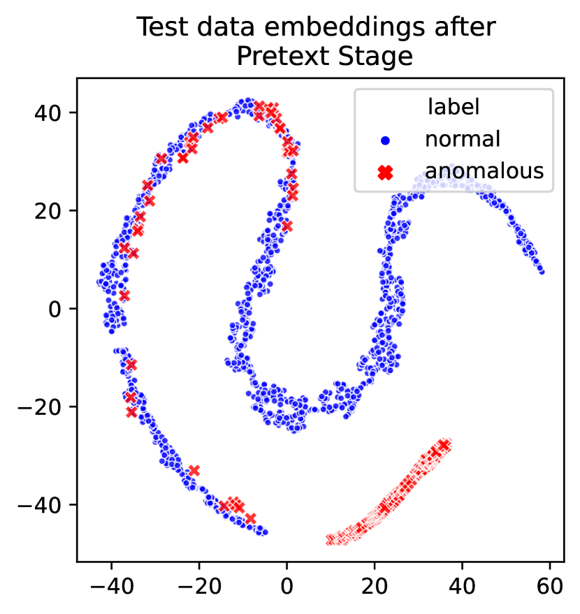
(a)

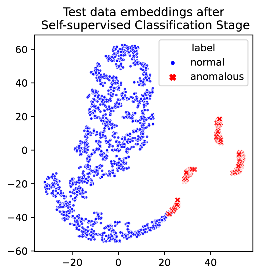
(b)

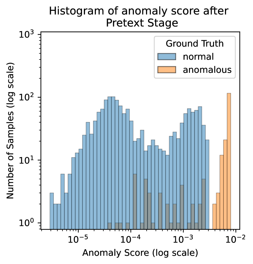
(c)

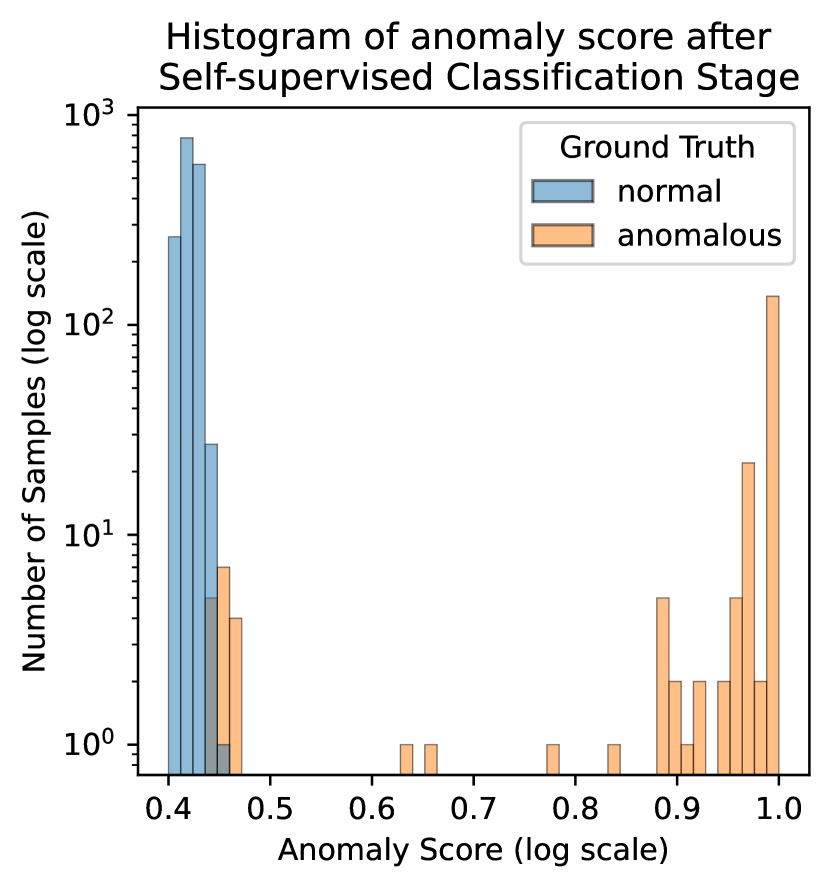
(d)

Figure 4: Comparative analysis of the model’s stages utilising t-SNE and anomaly score distributions on M-6 dataset in MSL. (a) t-SNE after the Pretext stage, indicating the initial representation of normal and anomalous samples. (b) t-SNE after the Self-supervised Classification stage, demonstrating enhanced segregation of normal and anomalous instances. (c) Anomaly score distribution in the Pretext Stage based on Euclidean distances between test and training samples. (d) The distribution of anomaly scores following the application of the Self-supervised Classification Stage, evidencing an improved representation.

Further, we assessed the efficacy of the Self-supervised Classification Stage in refining the representation generated by the Pretext Stage. This was accomplished by juxtaposing the anomaly scores derived from the output of each stage. In Fig. 4(c), the distribution of anomaly scores for the test windows at the Pretext Stage is displayed, computed using the Euclidean distances of the test samples relative to the original time series windows in the training set. Conversely, Fig. 4(d) depicts the subsequent alteration in the distribution of anomaly scores following the application of the Self-supervised Classification.

In the Pretext Stage, the anomaly score is computed as the minimum distance between the test sample and all original training samples in the representation space. This approach aims to identify the closest match among the training samples for the given test sample. A smaller distance implies a greater probability that the test sample belongs from the normal data distribution.

In the Self-supervised Classification Stage, we use inference step in Section III-C of the article. Equation 8 provides further details on the computation of the anomaly label.

As we can observe from the Fig. 4(d), the self-supervised classification Stage has resulted in a significant improvement in the separation of normal and anomalous windows. The distribution of anomaly scores in Fig. 4(d) is more clearly separated than in Fig. 4(c). This indicates that the second stage has produced more consistent representations. Furthermore, the anomaly scores in Fig. 4(d) are relatively closer to 0 or 1, which indicates an improvement in discrimination between normal and anomalous windows in the second stage of CARLA.

IV-E2 Positive Pair Selection

To evaluate the effectiveness of the positive pair selection method in CARLA we compared two approaches in training:: random temporal neighbour from $y$ temporally closest window samples and weak augmentation with noise (add normal noise with sigma 0.01 to a window). We used MSL benchmark and using identical configuration and hyper-parameters for both approaches and evaluated their performance shown in Table IV.

TABLE IV: Positive pair selection results on MSL dataset.

Pos Pair Selection	Prec	Rec	F1	AU-PR
CARLA-noise	0.3086	0.7935	0.4433	0.3983
CARLA-temporal	0.3891	0.7959	0.5227	0.5009

Our experiment demonstrated that selecting positive pairs using a random temporal neighbour is a more effective approach than weak augmentation with noise. Since anomalies occur rarely, choosing a positive pair that is in target window’s temporal proximity is a better strategy in our model.

IV-E3 Effectiveness of Different Anomaly Types

Based on the results of the ablation study on the MSL dataset, CARLA’s performance is evaluated by systematically removing different types of anomalies during the Pretext Stage. The evaluation metrics used are precision, recall, F1 score, and AU-PR. The results are sorted based on F1 from the least significant to the most significant types of anomalies in Table V. This result represents the overall performance of the CARLA model when using all types of anomalies during the anomaly injection process. It serves as a baseline for comparison with the subsequent results.

TABLE V: Effectiveness of different anomaly types on MSL dataset.

Anomaly Type	Prec	Rec	F1	AU-PR
All types	0.3891	0.7959	0.5227	0.5009
w/o trend	0.3185	0.7849	0.4513	0.4972
w/o contextual	0.3842	0.7935	0.5177	0.4683
w/o shapelet	0.3564	0.8370	0.4999	0.4328
w/o global	0.3383	0.8404	0.4824	0.4340
w/o seasonal	0.2400	0.8428	0.3737	0.3541

In the experiments, anomalies were injected into the training data on a per-window basis. For each window in the multivariate time series, a random number of dimensions was selected, ranging from 1 to $\lceil Dim/10\rceil$ of the total dimensions. These selected dimensions were injected with anomalies, starting from the same point across all the chosen dimensions. The injected anomaly portion for each dimension varied from 1 data point to 90% of the window length. This approach ensured a diverse and controlled injection of anomalies within the training data (For more detail see Algorithm 1)

Eliminating trend anomalies has a significant negative impact on CARLA’s precision. However, the recall remains relatively high, indicating that trend anomalies are important for maintaining a higher precision level. Similar to the previous case, removing contextual anomalies leads to a slight decrease in precision but an improvement in recall. The exclusion of shapelet anomalies leads to a moderate decrease in precision, while the recall remains relatively high. This suggests that shapelet anomalies contribute to the model’s precision but are not as crucial for capturing anomalies in general.

By removing global anomalies, CARLA’s precision slightly decreases, indicating that it becomes less accurate in identifying true anomalies. However, the recall improves, suggesting that the model becomes more sensitive in detecting anomalies overall. Removing seasonal anomalies has a noticeable effect on the model’s precision, which drops significantly. The consistently high recall suggests the model effectively captures many anomalies without relying on seasonal patterns.

Overall, the analysis of the results suggests that global and seasonal anomalies play a relatively more significant role in the CARLA model’s performance, while contextual, shapelet, and trend anomalies have varying degrees of impact. These findings provide insights into the model’s sensitivity to different types of anomalies and can guide further improvements in anomaly injection strategies within CARLA’s framework.

IV-E4 Effectiveness of Loss Components

To assess the effectiveness of two loss components, namely $\mathcal{L}_{inconsistency}$ and $\mathcal{L}_{entropy}$, in the total loss function for self-supervised classification on the MSL dataset, we conduct experiments using identical architecture and hyper-parameters. The evaluation metrics employed to measure the performance are precision, recall, F1 score, and AU-PR, as presented in Table VI.

TABLE VI: Effectiveness of $\mathcal{L}_{inconsistency}$ and $\mathcal{L}_{entropy}$ on MSL dataset.

$\mathcal{L}_{inconsistency}$	$\mathcal{L}_{entropy}$	Prec	Rec	F1	AU-PR
✗	✗	0.3092	0.7155	0.4318	0.3984
✗	✓	0.3453	0.8112	0.4846	0.4424
✓	✗	0.3219	0.7534	0.4511	0.4175
✓	✓	0.3891	0.7959	0.5227	0.5009

In cases where only one loss component is used the model’s performance is relatively lower across all metrics, indicating that without incorporating these loss components, the model struggles to effectively detect anomalies in the MSL dataset.

Where both $\mathcal{L}_{inconsistency}$ and $\mathcal{L}_{entropy}$ loss components are included in the total loss function, the model achieves the best performance among all scenarios, surpassing the other combinations. The precision, recall, F1 score, and AU-PR are the highest in this case, indicating that the combination of both loss components significantly improves the anomaly detection capability of the model.

IV-F Parameter Sensitivity

We also examine the sensitivity of CARLA’s parameters. We investigate and analyze the effect of the window size, number of classes, number of NN/FN, and coefficient of entropy.

IV-F1 Effect of Window Size

As a hyper-parameter in time series analysis, window size holds considerable importance. Table VII and Fig. 6 present the results of exploring the impact of window size on three datasets: MSL, SMD, and Yahoo.

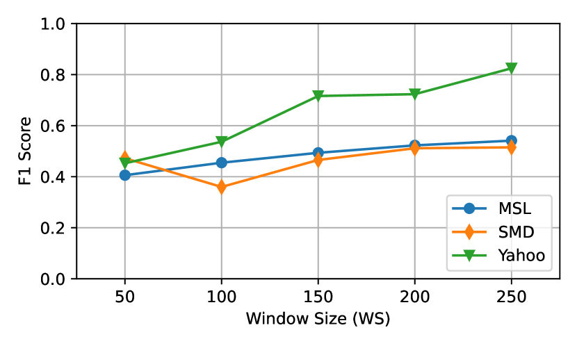
(a)

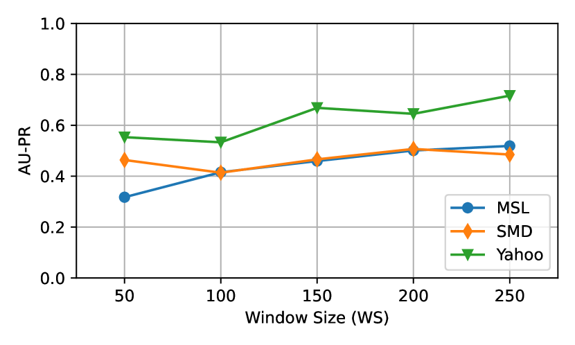
(b)

Figure 5: (a) F1 Score and (b) AU-PR for different Window sizes across MSL, SMD, and Yahoo datasets

TABLE VII: Exploring the effect of window size on MSL, SMD, and Yahoo datasets.

	MSL				SMD				Yahoo
WS	Prec	Rec	F1	AUPR	Prec	Rec	F1	AUPR	Prec	Rec	F1	AUPR
50	0.2755	0.7702	0.4058	0.3173	0.4569	0.4885	0.4722	0.4636	0.3046	0.8800	0.4526	0.5533
100	0.3233	0.7666	0.4548	0.4155	0.2584	0.5938	0.3598	0.4136	0.3709	0.9713	0.5368	0.5331
150	0.3606	0.7823	0.4936	0.4595	0.3599	0.6592	0.4655	0.4661	0.5720	0.9578	0.7162	0.6685
200	0.3891	0.7959	0.5227	0.5009	0.4276	0.6362	0.5114	0.5070	0.5747	0.9755	0.7233	0.6450
250	0.4380	0.8037	0.5412	0.5188	0.4224	0.6596	0.5150	0.4850	0.7129	0.9781	0.8247	0.7164

Based on the analysis of both the F1 score and AU-PR, it can be concluded that window size 200 consistently outperforms other window sizes on the MSL, SMD, and Yahoo datasets overall. This window size strikes a balance between precision and recall, effectively capturing anomalies while maintaining a high discrimination ability. Therefore, window size 200 is selected as the best choice for conducting time series analysis in all experiments. Additionally, Fig. 6 shows that our model’s performance is stable in window sizes between 150 to 250.

IV-F2 Effect of Number of Classes

The provided results showcase the performance of the model with varying numbers of classes on the MSL dataset.

Based on the illustration of both the F1 score and AU-PR in Fig. 6(a), the model performs relatively well across different numbers of classes. While CARLA’s performance is pretty stable across all number of classes denoted on x-axis of the plot in Fig. 6(a), it can be concluded that using 10 classes as the number of class parameter yields the highest performance. It strikes a balance between capturing anomalies and minimising false positives, while effectively discriminating between anomalies and normal data points.

The results suggest that increasing the number of classes beyond 10 does not significantly improve the model’s performance. When the number of classes increases, normal representations divide into the different classes and in CARLA detected as anomalies (lower probability of belonging to the major class). However, using 2 classes leads to a lower performance compared to the selected parameter of 10 classes, implying that a more fine-grained classification with 10 classes provides the assumption that various anomalies are spread in the representation space.

IV-F3 Effect of Number of neighbours in $\mathcal{N}$ and $\mathcal{F}$

The provided results in Fig. 6(b) display the evaluation metrics for different numbers of nearest neighbours ($\mathcal{N}$) and furthest neighbours ($\mathcal{F}$) noted as $Q$.

Based on the analysis of both the F1 score and AU-PR, we can see that while CARLA’s performance is pretty stable across different number of neighbours in $\mathcal{N}$ and $\mathcal{F}$ denoted on x-axis of the plot in Fig. 6(b), it can be concluded that employing 5 nearest/furthest neighbours outperforms the other options. This number of parameters strikes a favourable balance between precision and recall, allowing for effective anomaly detection while maintaining a high discrimination ability. Therefore, selecting 5 for the number of neighbours is deemed the optimal choice for this experiment, as it consistently achieves higher F1 scores and AU-PR values.

IV-F4 Effect of Coefficient of Entropy

In this experiment we explore the impact of the entropy coefficient. Fig. 6(c) shows the results of evaluating the coefficient of the entropy component in the loss function on the MSL dataset. The coefficients tested are 0, 2, 5, and 10.

Based on the analysis of both the F1 score and AU-PR, a coefficient value of 5 emerges as the most effective choice for the entropy component in the loss function. It achieves the highest scores for both metrics, indicating better precision-recall balance and accurate ranking of anomalies. However, it is worth noting that coefficients of 2 and 10 also demonstrate competitive performance, slightly lower than the value of 5. The coefficient of 0 significantly reduces the model’s performance, further emphasising the importance of incorporating the entropy component for improved anomaly detection performance.

Overall, the analysis indicates that coefficients of 2, 5, and 10 are viable for the entropy component in the loss function, but a coefficient of 5 is chosen as optimal due to its superior F1 score and AU-PR.

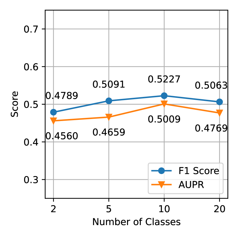
(a)

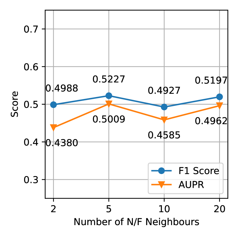
(b)

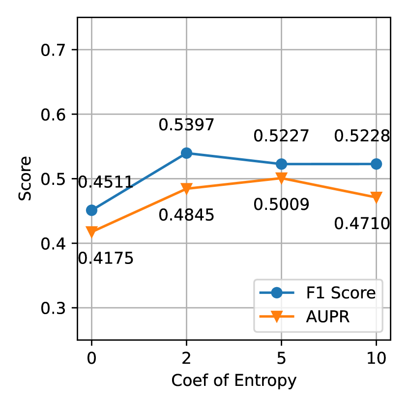
(c)

Figure 6: F1 Score and AU-PR for (a) different number of classes, (b) different numbers of neighbours in $\mathcal{N}$/$\mathcal{F}$ and (c) different coefficient of entropy, on MSL dataset.

V Point Adjustment (PA)

A notable issue with many existing Time Series Anomaly Detection (TAD) methods is their reliance on a specific evaluation approach called point adjustment (PA) strategy [71], and utilised in TAD literature such as [18], [6], and [31]. PA operates under the following principle: if a given segment is detected as anomalous, all previous segments in that anomaly subsequence are considered as anomalies (see Fig. 7). PA was introduced under the assumption that a solitary alert during an anomaly phase is adequate to recover the system. It has evolved into a fundamental stage in the assessment of TAD, with certain studies exclusively documenting $F1_{PA}$ without the conventional F1 score [72]. A higher $F1_{PA}$ is often interpreted as indicating better detection capability.

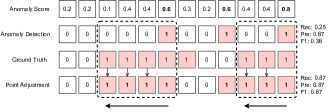
Figure 7: Impact of point adjustment (PA). The figure shows anomaly scores for 12 sequence samples. The second row displays results using a 0.5 threshold on all scores. The third row has actual labels (ground truth). The fourth row presents adjusted results using PA with the ground truth.

In Fig. 7, for the unadjusted detection, we have True Positives (TP): 2, True Negatives (TN): 3, False Positives (FP): 1, False Negatives (FN): 6, yielding a Recall of 0.25, Precision of 0.67, and F1 score of 0.36. In contrast, the adjusted detection (in bold for emphasis) resulted in TP: 7, TN: 3, FP: 1, and FN: 1, giving a significantly improved Recall of 0.875, Precision of 0.875, and F1 score of 0.875. This illustrates the substantial difference in evaluation results due to the application of PA in the anomaly detection process. It is evident that the PA greatly enhances the performance of anomaly detection.

TABLE VIII: Precision ($Prec_{PA}$), recall ($Rec_{PA}$), and $F1_{PA}$ results with point adjustment (PA) for various models on multivariate time series datasets.

Dataset	Metric	OmniAnomaly	THOC	TS2Vec	DCdetector	Random	CARLA
MSL	$Prec_{PA}$	0.8241	0.8291	0.2152	0.9369	0.1746	0.8545
	$Rec_{PA}$	0.9859	0.9651	1.0000	0.9969	1.0000	0.9650
	$F1_{PA}$	0.8978	0.8919	0.3542	0.9660	0.9840	0.9064
SMAP	$Prec_{PA}$	0.6931	0.5741	0.2605	0.9563	0.9740	0.7342
	$Rec_{PA}$	0.9754	0.9324	1.0000	0.9892	1.0000	0.9935
	$F1_{PA}$	0.8104	0.7106	0.4133	0.9702	0.9869	0.8444
SMD	$Prec_{PA}$	0.8193	0.3819	0.1800	0.8359	0.8670	0.6757
	$Rec_{PA}$	0.9531	0.8946	0.9950	0.9110	0.9686	0.8465
	$F1_{PA}$	0.8811	0.5353	0.3050	0.8718	0.9150	0.7515
SWaT	$Prec_{PA}$	0.9861	0.7854	0.1718	0.6998	0.9398	0.9891
	$Rec_{PA}$	0.7864	0.9774	1.0000	0.9125	0.9331	0.7132
	$F1_{PA}$	0.8750	0.8709	0.2932	0.7921	0.9364	0.8288
WADI	$Prec_{PA}$	0.2685	0.3871	0.0893	0.2257	0.8627	0.1971
	$Rec_{PA}$	0.9686	0.7638	1.0000	0.9263	0.9732	0.7503
	$F1_{PA}$	0.4204	0.5138	0.1639	0.3630	0.9146	0.3122

TABLE IX: Precision ($Prec_{PA}$), recall ($Rec_{PA}$), and $F1_{PA}$ results with point adjustment (PA) for various models on univariate time series datasets.

Dataset	Metric	Donut	THOC	TS2Vec	Random	CARLA
Yahoo-A1	$Prec_{PA}$	0.5252	0.3138	0.4993	0.9020	0.7475
	$Rec_{PA}$	0.9280	0.9723	0.9717	0.9911	0.9984
	$F1_{PA}$	0.6883	0.4745	0.6597	0.9445	0.8549
KPI	$Prec_{PA}$	0.3928	0.3703	0.4514	0.6540	0.3980
	$Rec_{PA}$	0.5797	0.9154	0.9058	0.8986	0.8933
	$F1_{PA}$	0.4683	0.5273	0.6025	0.7570	0.5507

However, PA carries a notable peril of inflating the performance of the model. In most of the TAD models, an anomaly score is produced to indicate the degree of abnormality and the model detects a given point as an anomaly when the score surpasses a predefined threshold. Incorporating PA, the predictions based on the model that randomly generated anomaly scores uniformly outperforms all state-of-the-art models, as depicted in Tables VIII and IX. It becomes challenging to assert that a model with a superior $F1_{PA}$ performs better than a model with a lower $F1_{PA}$ when random anomaly scores have the potential to result a high $F1_{PA}$ comparable to that of a proficient detection model. Experimental results in Tables VIII and IX demonstrate that random anomaly score model can outperform all state-of-the-art models, highlighting the limitations of relying solely on $F1_{PA}$ for model evaluation.

VI Conclusion

In conclusion, our self-supervised framework CARLA effectively detects anomalies in time series data using contrastive representation learning. It demonstrates strong performance on seven key real-world datasets. This research highlights the potential of contrastive learning in addressing the challenges posed by unlabeled data in anomaly detection. Future improvements could include experimenting with various forms and severities of injected anomalies. Our findings, evaluated using metrics like the F1 score and AU-PR, provide a benchmark for future research in this area, particularly for datasets like WADI and KPI. These results are significant for advancing time series anomaly detection, offering a reliable basis for future model evaluation and innovation in the field.

References

- [1] F. E. Grubbs, “Procedures for detecting outlying observations in samples,” Technometrics, vol. 11, no. 1, pp. 1–21, 1969.
- [2] W. A. Shewhart, Economic control of manufactured product. van Nostrand, 1931.
- [3] M. Salehi, C. Leckie, J. C. Bezdek, T. Vaithianathan, and X. Zhang, “Fast memory efficient local outlier detection in data streams (extended abstract),” in 2017 IEEE 33rd International Conference on Data Engineering (ICDE), 2017, pp. 51–52.
- [4] G. Pang, C. Shen, L. Cao, and A. V. D. Hengel, “Deep learning for anomaly detection: A review,” ACM computing surveys (CSUR), vol. 54, no. 2, pp. 1–38, 2021.
- [5] Z. Z. Darban, G. I. Webb, S. Pan, C. C. Aggarwal, and M. Salehi, “Deep learning for time series anomaly detection: A survey,” arXiv preprint arXiv:2211.05244, 2022.
- [6] L. Shen, Z. Li, and J. Kwok, “Timeseries anomaly detection using temporal hierarchical one-class network,” Advances in Neural Information Processing Systems, vol. 33, pp. 13 016–13 026, 2020.
- [7] Z. Yue, Y. Wang, J. Duan, T. Yang, C. Huang, Y. Tong, and B. Xu, “Ts2vec: Towards universal representation of time series,” in Proceedings of the AAAI Conference on Artificial Intelligence, vol. 36, no. 8, 2022, pp. 8980–8987.
- [8] K. Hundman, V. Constantinou, C. Laporte, I. Colwell, and T. Soderstrom, “Detecting spacecraft anomalies using lstms and nonparametric dynamic thresholding,” in Proceedings of the 24th ACM SIGKDD international conference on knowledge discovery & data mining, 2018, pp. 387–395.
- [9] T. Chen, S. Kornblith, M. Norouzi, and G. Hinton, “A simple framework for contrastive learning of visual representations,” in International conference on machine learning. PMLR, 2020, pp. 1597–1607.
- [10] J. Giorgi, O. Nitski, B. Wang, and G. Bader, “Declutr: Deep contrastive learning for unsupervised textual representations,” arXiv preprint arXiv:2006.03659, 2020.
- [11] S. Schmidl, P. Wenig, and T. Papenbrock, “Anomaly detection in time series: a comprehensive evaluation,” Proceedings of the VLDB Endowment, vol. 15, no. 9, pp. 1779–1797, 2022.
- [12] J. Audibert, P. Michiardi, F. Guyard, S. Marti, and M. A. Zuluaga, “Do deep neural networks contribute to multivariate time series anomaly detection?” Pattern Recognition, vol. 132, p. 108945, 2022.
- [13] P. C. Phillips and S. Jin, “Business cycles, trend elimination, and the hp filter,” International Economic Review, vol. 62, no. 2, pp. 469–520, 2021.
- [14] G. E. Box and D. A. Pierce, “Distribution of residual autocorrelations in autoregressive-integrated moving average time series models,” Journal of the American Statistical Association, vol. 65, no. 332, pp. 1509–1526, 1970.
- [15] N. Kant and M. Mahajan, “Time-series outlier detection using enhanced k-means in combination with pso algorithm,” in Engineering Vibration, Communication and Information Processing: ICoEVCI 2018, India. Springer, 2019, pp. 363–373.
- [16] W. P. Paweł Karczmarek, Adam Kiersztyn and E. Al, “K-means-based isolation forest,” Knowledge-based systems, vol. 195, p. 105659, 2020.
- [17] K. M. T. Fei Tony Liu and Z.-H. Zhou, “Isolation forest,” in 2008 eighth IEEE international conference on data mining. IEEE, 2008, pp. 413–422.
- [18] J. Audibert, P. Michiardi, F. Guyard, S. Marti, and M. A. Zuluaga, “Usad: Unsupervised anomaly detection on multivariate time series,” in Proceedings of the 26th ACM SIGKDD International Conference on Knowledge Discovery & Data Mining, 2020, pp. 3395–3404.
- [19] Y. Li, X. Peng, J. Zhang, Z. Li, and M. Wen, “Dct-gan: dilated convolutional transformer-based gan for time series anomaly detection,” IEEE Transactions on Knowledge and Data Engineering, 2021.
- [20] J. Xu, H. Wu, J. Wang, and M. Long, “Anomaly transformer: Time series anomaly detection with association discrepancy,” arXiv preprint arXiv:2110.02642, 2021.
- [21] C. U. Carmona, F.-X. Aubet, V. Flunkert, and J. Gasthaus, “Neural contextual anomaly detection for time series,” arXiv preprint arXiv:2107.07702, 2021.
- [22] S. Chauhan and L. Vig, “Anomaly detection in ecg time signals via deep long short-term memory networks,” in 2015 IEEE international conference on data science and advanced analytics (DSAA). IEEE, 2015, pp. 1–7.
- [23] Z. Niu, K. Yu, and X. Wu, “Lstm-based vae-gan for time-series anomaly detection,” Sensors, vol. 20, no. 13, p. 3738, 2020.
- [24] D. Park, Y. Hoshi, and C. C. Kemp, “A multimodal anomaly detector for robot-assisted feeding using an lstm-based variational autoencoder,” IEEE Robotics and Automation Letters, vol. 3, no. 3, pp. 1544–1551, 2018.
- [25] P. Malhotra, L. Vig, G. Shroff, and P. Agarwal, “Lstm-based encoder-decoder for multi-sensor anomaly detection,” in International conference on machine learning, 2016, pp. 1724–1732.
- [26] M. Giannoulis, A. Harris, and V. Barra, “Ditan: A deep-learning domain agnostic framework for detection and interpretation of temporally-based multivariate anomalies,” Pattern Recognition, vol. 143, p. 109814, 2023.
- [27] B. Zong, Q. Song, M. R. Min, W. Cheng, C. Lumezanu, D. Cho, and H. Chen, “Deep autoencoding gaussian mixture model for unsupervised anomaly detection,” in International conference on learning representations, 2018.
- [28] C. Zhang, D. Song, Y. Chen, X. Feng, C. Lumezanu, W. Cheng, J. Ni, B. Zong, H. Chen, and N. V. Chawla, “A deep neural network for unsupervised anomaly detection and diagnosis in multivariate time series data,” in Proceedings of the AAAI conference on artificial intelligence, vol. 33, no. 01, 2019, pp. 1409–1416.
- [29] X. Chen, L. Deng, F. Huang, C. Zhang, Z. Zhang, Y. Zhao, and K. Zheng, “Daemon: Unsupervised anomaly detection and interpretation for multivariate time series,” in 2021 IEEE 37th International Conference on Data Engineering (ICDE). IEEE, 2021, pp. 2225–2230.
- [30] Y. Yao, J. Ma, and Y. Ye, “Regularizing autoencoders with wavelet transform for sequence anomaly detection,” Pattern Recognition, vol. 134, p. 109084, 2023.
- [31] Y. Su, Y. Zhao, C. Niu, R. Liu, W. Sun, and D. Pei, “Robust anomaly detection for multivariate time series through stochastic recurrent neural network,” in Proceedings of the 25th ACM SIGKDD international conference on knowledge discovery & data mining, 2019, pp. 2828–2837.
- [32] D. Li, D. Chen, B. Jin, L. Shi, J. Goh, and S.-K. Ng, “Mad-gan: Multivariate anomaly detection for time series data with generative adversarial networks,” in Artificial Neural Networks and Machine Learning–ICANN 2019: Text and Time Series: 28th International Conference on Artificial Neural Networks, Munich, Germany, September 17–19, 2019, Proceedings, Part IV. Springer, 2019, pp. 703–716.
- [33] B. Zhou, S. Liu, B. Hooi, X. Cheng, and J. Ye, “Beatgan: Anomalous rhythm detection using adversarially generated time series.” in IJCAI, vol. 2019, 2019, pp. 4433–4439.
- [34] N. Kodali, J. Abernethy, J. Hays, and Z. Kira, “On convergence and stability of gans,” arXiv preprint arXiv:1705.07215, 2017.
- [35] M. Sakurada and T. Yairi, “Anomaly detection using autoencoders with nonlinear dimensionality reduction,” in Proceedings of the MLSDA 2014 2nd Workshop on Machine Learning for Sensory Data Analysis, 2014, pp. 4–11.
- [36] M. Canizo, I. Triguero, A. Conde, and E. Onieva, “Multi-head cnn–rnn for multi-time series anomaly detection: An industrial case study,” Neurocomputing, vol. 363, pp. 246–260, 2019.
- [37] Y. Yang, C. Zhang, T. Zhou, Q. Wen, and L. Sun, “Dcdetector: Dual attention contrastive representation learning for time series anomaly detection,” in Proc. 29th ACM SIGKDD International Conference on Knowledge Discovery & Data Mining (KDD 2023), 2023.
- [38] H. Deng, Y. Sun, M. Qiu, C. Zhou, and Z. Chen, “Graph neural network-based anomaly detection in multivariate time series data,” in 2021 IEEE 45th Annual Computers, Software, and Applications Conference (COMPSAC). IEEE, 2021, pp. 1128–1133.
- [39] L. Li, J. Yan, Q. Wen, Y. Jin, and X. Yang, “Learning robust deep state space for unsupervised anomaly detection in contaminated time-series,” IEEE Transactions on Knowledge and Data Engineering, 2022.
- [40] Y. Jiao, K. Yang, D. Song, and D. Tao, “Timeautoad: Autonomous anomaly detection with self-supervised contrastive loss for multivariate time series,” IEEE Transactions on Network Science and Engineering, vol. 9, no. 3, pp. 1604–1619, 2022.
- [41] Y. Zhang, J. Wang, Y. Chen, H. Yu, and T. Qin, “Adaptive memory networks with self-supervised learning for unsupervised anomaly detection,” IEEE Transactions on Knowledge and Data Engineering, 2022.
- [42] H. Zhao, Y. Wang, J. Duan, C. Huang, D. Cao, Y. Tong, B. Xu, J. Bai, J. Tong, and Q. Zhang, “Multivariate time-series anomaly detection via graph attention network,” in 2020 IEEE International Conference on Data Mining (ICDM). IEEE, 2020, pp. 841–850.
- [43] X. Wang, R. Zhang, C. Shen, T. Kong, and L. Li, “Dense contrastive learning for self-supervised visual pre-training,” in Proc. IEEE Conf. Computer Vision and Pattern Recognition (CVPR). IEEE, 2021.
- [44] H. Xu, X. Zhang, H. Li, L. Xie, H. Xiong, and Q. Tian, “Hierarchical semantic aggregation for contrastive representation learning,” arXiv preprint arXiv:2012.02733, 2020.
- [45] P. O. Pinheiro, A. Almahairi, R. Benmalek, F. Golemo, and A. C. Courville, “Unsupervised learning of dense visual representations,” in Advances in Neural Information Processing Systems, vol. 33. Curran Associates, Inc., 2020, pp. 4489–4500.
- [46] T. Gao, X. Yao, and D. Chen, “Simcse: Simple contrastive learning of sentence embeddings,” arXiv preprint arXiv:2104.08821, 2021.
- [47] L. Logeswaran and H. Lee, “An efficient framework for learning sentence representations,” in International Conference on Learning Representations, 2018.
- [48] A. Baevski, Y. Zhou, A. Mohamed, and M. Auli, “wav2vec 2.0: A framework for self-supervised learning of speech representations,” Advances in Neural Information Processing Systems, vol. 33, 2020.
- [49] Q. Xu, A. Baevski, T. Likhomanenko, P. Tomasello, A. Conneau, R. Collobert, G. Synnaeve, and M. Auli, “Self-training and pre-training are complementary for speech recognition,” in ICASSP 2021-2021 IEEE International Conference on Acoustics, Speech and Signal Processing (ICASSP). IEEE, 2021, pp. 3030–3034.
- [50] Q. Lei, J. Yi, R. Vaculin, L. Wu, and I. S. Dhillon, “Similarity preserving representation learning for time series clustering,” in International Joint Conference on Artificial Intelligence, vol. 19, 2019, pp. 2845–2851.
- [51] P. Malhotra, V. TV, L. Vig, P. Agarwal, and G. Shroff, “Timenet: Pre-trained deep recurrent neural network for time series classification,” arXiv preprint arXiv:1706.08838, 2017.
- [52] L. Wu, I. E.-H. Yen, J. Yi, F. Xu, Q. Lei, and M. Witbrock, “Random warping series: A random features method for time-series embedding,” in International Conference on Artificial Intelligence and Statistics. PMLR, 2018, pp. 793–802.
- [53] F. M. Bianchi, L. Livi, K. Ø. Mikalsen, M. Kampffmeyer, and R. Jenssen, “Learning representations of multivariate time series with missing data,” Pattern Recognition, vol. 96, p. 106973, 2019.
- [54] G. Zerveas, S. Jayaraman, D. Patel, A. Bhamidipaty, and C. Eickhoff, “A transformer-based framework for multivariate time series representation learning,” in Proceedings of the 27th ACM SIGKDD Conference on Knowledge Discovery & Data Mining. Association for Computing Machinery, 2021, pp. 2114–2124.
- [55] S. Tonekaboni, D. Eytan, and A. Goldenberg, “Unsupervised representation learning for time series with temporal neighborhood coding,” in International Conference on Learning Representations, 2021.
- [56] J.-Y. Franceschi, A. Dieuleveut, and M. Jaggi, “Unsupervised scalable representation learning for multivariate time series,” in Advances in Neural Information Processing Systems, vol. 32. Curran Associates, Inc., 2019.
- [57] G. Pang, L. Cao, L. Chen, and H. Liu, “Learning representations of ultrahigh-dimensional data for random distance-based outlier detection,” in Proceedings of the 24th ACM SIGKDD international conference on knowledge discovery & data mining, 2018, pp. 2041–2050.
- [58] E. Eldele, M. Ragab, Z. Chen, M. Wu, C. K. Kwoh, X. Li, and C. Guan, “Time-series representation learning via temporal and contextual contrasting,” in Proceedings of the Thirtieth International Joint Conference on Artificial Intelligence, 2021, pp. 2352–2359.
- [59] P. H. Le-Khac, G. Healy, and A. F. Smeaton, “Contrastive representation learning: A framework and review,” Ieee Access, vol. 8, pp. 193 907–193 934, 2020.
- [60] A. v. d. Oord, Y. Li, and O. Vinyals, “Representation learning with contrastive predictive coding,” arXiv preprint arXiv:1807.03748, 2018.
- [61] M. Caron, I. Misra, J. Mairal, P. Goyal, P. Bojanowski, and A. Joulin, “Unsupervised learning of visual features by contrasting cluster assignments,” Advances in neural information processing systems, vol. 33, pp. 9912–9924, 2020.
- [62] K. He, H. Fan, Y. Wu, S. Xie, and R. Girshick, “Momentum contrast for unsupervised visual representation learning,” in Proceedings of the IEEE/CVF conference on computer vision and pattern recognition, 2020, pp. 9729–9738.
- [63] J.-B. Grill, F. Strub, F. Altché, C. Tallec, P. Richemond, E. Buchatskaya, C. Doersch, B. A. Pires, Z. Guo, M. G. Azar et al., “Bootstrap your own latent-a new approach to self-supervised learning,” Advances in neural information processing systems, vol. 33, pp. 21 271–21 284, 2020.
- [64] X. Chen and K. He, “Exploring simple siamese representation learning,” in Proceedings of the IEEE/CVF Conference on Computer Vision and Pattern Recognition, 2021, pp. 15 750–15 758.
- [65] K.-H. Lai, D. Zha, J. Xu, Y. Zhao, G. Wang, and X. Hu, “Revisiting time series outlier detection: Definitions and benchmarks,” in Thirty-fifth Conference on Neural Information Processing Systems Datasets and Benchmarks Track (Round 1), 2021.
- [66] D. Hendrycks, M. Mazeika, and T. Dietterich, “Deep anomaly detection with outlier exposure,” arXiv preprint arXiv:1812.04606, 2018.
- [67] H. Ismail Fawaz, G. Forestier, J. Weber, L. Idoumghar, and P.-A. Muller, “Deep learning for time series classification: a review,” Data mining and knowledge discovery, vol. 33, no. 4, pp. 917–963, 2019.
- [68] A. P. Mathur and N. O. Tippenhauer, “Swat: A water treatment testbed for research and training on ics security,” in 2016 international workshop on cyber-physical systems for smart water networks (CySWater). IEEE, 2016, pp. 31–36.
- [69] C. M. Ahmed, V. R. Palleti, and A. P. Mathur, “Wadi: a water distribution testbed for research in the design of secure cyber physical systems,” in Proceedings of the 3rd international workshop on cyber-physical systems for smart water networks, 2017, pp. 25–28.
- [70] N. Laptev, Y. B., and S. Amizadeh, “A benchmark dataset for time series anomaly detection.” 2015. [Online]. Available: https://yahooresearch.tumblr.com/post/114590420346/a-benchmark-dataset-for-time-series-anomaly.
- [71] H. Xu, W. Chen, N. Zhao, Z. Li, J. Bu, Z. Li, Y. Liu, Y. Zhao, D. Pei, Y. Feng et al., “Unsupervised anomaly detection via variational auto-encoder for seasonal kpis in web applications,” in Proceedings of the 2018 world wide web conference, 2018, pp. 187–196.
- [72] S. Kim, K. Choi, H.-S. Choi, B. Lee, and S. Yoon, “Towards a rigorous evaluation of time-series anomaly detection,” in Proceedings of the AAAI Conference on Artificial Intelligence, vol. 36, no. 7, 2022, pp. 7194–7201.
- [73] T. Saito and M. Rehmsmeier, “The precision-recall plot is more informative than the roc plot when evaluating binary classifiers on imbalanced datasets,” PloS one, vol. 10, no. 3, p. e0118432, 2015.