Power spectrum with $k^{6}$ growth for primordial black holes

Abstract

The decrease of both the rolling speed of the inflaton and the sound speed of the curvature perturbations can amplify the curvature perturbations during inflation so as to generate a sizable amount of primordial black holes. In the ultraslow-roll inflation scenario, it has been found that the power spectrum of curvature perturbations has a $k^{4}$ growth. In this paper, we find that when the speed of sound decreases suddenly, the curvature perturbations becomes scale dependent in the infrared limit and the power spectrum of the curvature perturbation only has a $k^{2}$ growth. Furthermore, by studying the evolution of the power spectrum in the inflation model, in which both the sound speed of the curvature perturbations and the rolling speed of the inflaton are reduced, we find that the power spectrum is nearly scale invariant at the large scales to satisfy the constraint from the cosmic microwave background radiation observations, and at the same time can be enhanced at the small scales to result in an abundant formation of primordial black holes. In the cases of the simultaneous changes of the sound speed and the slow-roll parameter $\eta$ and the change of the sound speed preceding that of the slow-roll parameter $\eta$, the power spectrum can possess a $k^{6}$ growth under certain conditions, which is the steepest growth of the power spectrum reported so far.

I Introduction

During the standard slow-roll inflation, the solution of the Sasaki-Mukhanov equation for the evolution of the curvature perturbations $\mathcal{R}$ contains, in the infrared limit, a constant term and a time-decaying one, and this solution results in a nearly scale-invariant power spectrum of the curvature perturbations Bruce A. Bassett ; Antonio Riotto , which is well-consistent with the cosmic microwave background (CMB) radiation observations. The CMB observations have limited the amplitude of the power spectrum to the order of $\mathcal{O}(10^{-9})$ at the CMB scale Smoot1997 ; Spergel2003 ; Komatsu2011 ; Akrami2020 ; Aghanim2020 . It has been found that, if the amplitude of the power spectrum of the curvature perturbations can be enhanced for about seven orders at the scales smaller than the CMB one S. Chongchitnan ; K. Kohri ; C. T. Byrnes ; E. Bugaev , a sizable amount of primordial black holes can be generated when these enhanced perturbations reenter the horizon during the radiation- or matter-dominated era Zeldovich ; Hawking ; Carr ; Meszaros ; Carr1975 ; Khlopov ; Ozsoy2023 ; Bhattacharya2023b .

The amplitude of the power spectrum of the curvature perturbations in the standard slow-roll inflation can be expressed as $\mathcal{P_{R}}=\frac{H^{2}}{8\pi^{2}\epsilon c_{s}}$ when the mode exits the horizon during inflation, where $H$ is the Hubble parameter which is approximately constant during inflation, $\epsilon$ the slow-roll parameter and $c_{s}$ the sound speed of the curvature perturbations. Thus, a natural way to amplify the curvature perturbations is to reduce the rolling speed of the inflaton which is proportional to $\epsilon$ or to suppress the sound speed. Decreasing the inflaton’s rolling speed can be realized in the ultraslow-roll inflation Yokoyama1998 ; Choudhury2014 ; Germani2017 ; Motohashi2017 ; Ezquiaga2017 ; H. Di2018 ; Ballesteros2018 ; Dalianis2019 ; Gao2018 ; Tada2019 ; Mishra2020 ; Atal2020 ; Ragavendra2021 ; Bhaumik2020 ; Drees2021 ; C.Fu2020 ; Xu2020 ; Lin2020 ; Dalianis2021 ; Yi2021 ; Gao2021 ; Yi2021b ; TGao2021 ; Solbi2021 ; Gao2021b ; Solbi2021b ; Zheng2021 ; Teimoori2021a ; Cai2021 ; Wang2021 ; Fuchengjie2019 ; fuchengjie2020 ; Dalianis2020 ; Teimoori2021 ; Karam2022 ; Heydari2022 ; Heydari2022b ; Bellido2017 ; Ezquiaga2018 ; Pi2022 ; Choudhury2023 ; Meng2022 ; Mu2022 ; Kawaguchi2022 ; Fu2022 ; Chen2022 ; Gu2023 ; Yi2022 ; Choudhury2023c ; Choudhury2023e ; Choudhury2023b ; Cai2023 ; Ghoshal2023 ; Franciolini2023 , in which the slow-roll parameter $\eta$, which is defined to be $\eta=\frac{\dot{\epsilon}}{\epsilon H}$ with an overdot denoting a derivative with respect to the time $t$, equals approximately $-6$. During the transition of $\eta$ from $\eta\simeq 0$, which corresponds to the slow-roll inflation, to $-6$, the Israel junction conditions Israel1966 ; Deruelle1995 are used to obtain the solution of the curvature perturbations in the ultraslow-roll phase. Expanding this solution in the infrared limit, one can see that the decaying term in the solution of the Sasaki-Mukhanov equation for the evolution of the curvature perturbations becomes a growing one. This growing term gradually dominates if the ultraslow-roll inflation persists a sufficiently long time and it results in the enhancement of the curvature perturbations to meet the requirement of formation of a sizable amount of primordial black holes. It has been found that the power spectrum of the curvature perturbations displays a $k^{4}$ growth and has a dip preceding the $k^{4}$ dependence Garrilho2019 ; Liu2020 ; Byrnes2019 . The steeper $k^{5}(\log k)^{2}$ growth of the power spectrum can be obtained if an $\eta=-1$ middle phase between the slow- and ultraslow-roll inflations Garrilho2019 ; Cole2022 is added.

When the amplification of the curvature perturbations results from the decrease of the sound speed G. Ballesteros ; Kamenshchik ; Gorji2022 ; Romano3 ; Ballesteros2022 , which equals $1$ in the canonical scalar field inflation model, the solution of the curvature perturbations, although does not contain growing terms, still has a constant component and a decay part. However, the constant component becomes scale variant at small scales, which makes the power spectrum become enhanced. If the Israel junction conditions are utilized to match the curvature perturbation and its derivative at the time when the sound speed decreases suddenly, the power spectrum has a $k^{4}$ growth Ballesteros2022 ; Zhai2022 . However, this junction conditions is inapplicable in the case that the sound speed suddenly decreases due to the appearance of the square of the delta function Nakashima2011 . Therefore, in this paper we will employ an improved junction conditions Gorji2022 to restudy the evolution of the power spectrum when the sound speed decreases suddenly and find that the growth of the power spectrum is $k^{2}$ rather than $k^{4}$.

Furthermore, in the Dirac-Born-Infeld-inspired nonminimal kinetic coupling inflation model Qiu2022 , both $\epsilon$ and $c_{s}^{2}$ are closely related to the concrete form of the inflationary potential, which indicates that this inflation model may accommodate both a small sound speed of the curvature perturbations and a small rolling speed of the inflaton at the same time. When both the inflaton’s rolling speed and the sound speed of the curvature perturbations are suppressed during inflation, will the growth of the power spectrum of the curvature perturbations be steeper than $k^{4}$? This is an interesting problem, which we are also going to address in this paper.

The rest of this paper is organized as follows: In Sec. II, the evolution of the power spectrum is investigated when the speed of sound decreases suddenly. In Sec. III, we study the evolution of the power spectrum in the case that both the sound speed and the slow-roll parameter are suppressed and present our conclusions in Sec. IV. Throughout this paper, we set $c=\hbar=M_{\mathrm{Pl}}=1$.

II Growth of power spectrum from the sudden decrease of the sound speed

The evolution of the curvature perturbations $\mathcal{R}$ satisfies the Sasaki-Mukhanov equation, which in the Fourier space takes the form

$$v^{\prime\prime}_{k}+\left(c_{s}^{2}k^{2}-\frac{z^{\prime\prime}}{z}\right)v_{k}=0\;,$$ (1)

where $v_{k}=z\mathcal{R}_{k}$, a prime indicates a derivative with respect to the conformal time $\tau$, and $z$ is defined as

$$z^{2}\equiv\frac{2a^{2}\epsilon}{c_{s}^{2}}$$ (2)

with $a$ being the cosmic scale factor. From the definition of $z$, one can obtain

$$\frac{z^{\prime\prime}}{z}=(aH)^{2}\left(2-\epsilon+\frac{3}{2}\eta-3s+s^{2}+s\epsilon-s\eta+\frac{1}{4}\eta^{2}-\frac{1}{2}\eta\epsilon\right)\;.$$ (3)

Here $s=\frac{\dot{c}_{s}}{c_{s}H}$. During the (ultra)slow-roll inflation, one has $\epsilon\ll 1$, and thus $aH\simeq-\frac{1}{\tau}$. Then Eq. (1) can be rewritten as

$$v^{\prime\prime}_{k}+\left(c_{s}^{2}k^{2}-\frac{\nu^{2}-1/4}{(-\tau)^{2}}\right)v_{k}=0\;,$$ (4)

where

$$\nu\simeq\frac{3}{2}+\frac{1}{2}\eta-s\;.$$ (5)

If $\eta$ and $c_{s}$ are constants, Eq. (4) has a general solution

$$v_{k}(\tau)=\alpha\sqrt{-\tau}H_{\nu}^{(1)}(-c_{s}k\tau)+\beta\sqrt{-\tau}H_{\nu}^{(2)}(-c_{s}k\tau)\;.$$ (6)

Here $H_{\nu}^{(1)}$ and $H_{\nu}^{(2)}$ are the first and second Hankel functions, respectively, and $\alpha$ and $\beta$ are two constants.

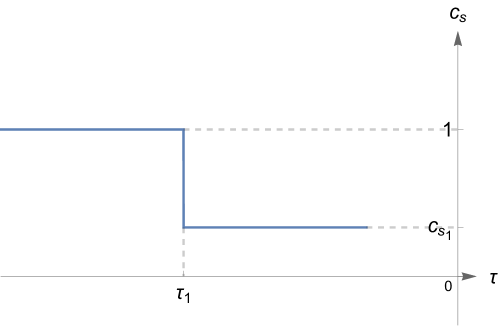
Figure 1: The sound speed $c_{s}$ varies suddenly at $\tau_{1}$.

Now, we discuss the scenario of a sudden decrease of the sound speed, as shown in Fig. 1. In the first stage ($\tau<\tau_{1}$), which corresponds to the canonical slow-roll inflation, the sound speed $c_{s}$ is equal to one and the slow-roll parameter $\eta$ is near zero. Thus, one has $\nu\simeq 3/2$ and $\epsilon=\epsilon_{0}(\frac{\tau}{\tau_{0}})^{-\eta}\simeq\epsilon_{0}$. Imposing that the solution of the Sasaki-Mukhanov equation matches the plane-wave form in the ultraviolet regime ($-k\tau\gg 1$), we can derive the evolution of the curvature perturbations

$$\mathcal{R}^{(0)}_{k}(\tau)=i\frac{H}{2\sqrt{\epsilon_{0}k^{3}}}e^{-ik\tau}(1+ik\tau)\;.$$ (7)

Apparently, the solution of the curvature perturbations contains a constant term and a time-decaying one since $|\tau|$ decreases with the cosmic expansion during inflation, which results in a nearly scale-invariant power spectrum of the curvature perturbations in the superhorizon scales ($-k\tau\rightarrow 0$) with the amplitude of the power spectrum being

$$\mathcal{P}_{0}=\frac{H^{2}}{8\pi^{2}\epsilon_{0}}\;.$$ (8)

The CMB observations have limited $\mathcal{P}_{0}$ to be $\sim 10^{-9}$ Smoot1997 . At the moment $\tau_{1}$, we assume that the sound speed decreases suddenly from 1 to a very tiny constant value $c_{s_{1}}$ and the inflation enters the second stage. In this stage, the general solution of the curvature perturbations has the form

$$\mathcal{R}^{(1)}_{k}(\tau)=\frac{ic_{s_{1}}H\left(-\tau\right)^{3/2}}{\sqrt{2\epsilon_{0}}}\left[\alpha_{1}H_{3/2}^{(1)}(c_{s_{1}}k\tau)+\beta_{1}H_{3/2}^{(2)}(c_{s_{1}}k\tau)\right]\;,$$ (9)

where $\alpha_{1}$ and $\beta_{1}$ are two constants. Usually, the Israel junction conditions $\mathcal{R}^{(0)}_{k}(\tau_{1})=\mathcal{R}^{(1)}_{k}(\tau_{1})$ and $\mathcal{R}^{\prime(0)}_{k}(\tau_{1})=\mathcal{R}^{\prime(1)}_{k}(\tau_{1})$ are used to determine the values of $\alpha_{1}$ and $\beta_{1}$ Ballesteros2022 ; Zhai2022 . However, it has been found, in Ref. Nakashima2011 , that there is a square term of the delta function $\delta(\tau-\tau_{1})$ arising form $(c_{s}^{\prime}/c_{s})^{2}$ in $z^{\prime\prime}/z$ when a sudden variation of the sound velocity occurs, which makes the analysis impossible, and thus the Israel junction conditions need to be modified or a new variable has to be introduced. In Nakashima2011 , a new variable is defined, which satisfies the Israel junction conditions at $\tau_{1}$. Here, we do not use this new variable Nakashima2011 but consider an improved junction conditions, i.e. $\mathcal{R}_{k}$ and its conjugate momentum $A\mathcal{R}^{\prime}_{k}$ are continuous at $\tau_{1}$, where $A\equiv\frac{2\epsilon}{c_{s}^{2}}$  Gorji2022 . We have checked that the introduction of the new viable and the improved junction conditions can give the same results. Considering the improved junction conditions

$$\mathcal{R}^{(0)}_{k}(\tau_{1})=\mathcal{R}^{(1)}_{k}(\tau_{1})\;,\quad A_{0}\mathcal{R}^{\prime(0)}_{k}(\tau_{1})=A_{1}\mathcal{R}^{\prime(1)}_{k}(\tau_{1})\;$$ (10)

with

$$A_{0}=2\epsilon_{0}\;,\quad A_{1}=\frac{2\epsilon_{0}}{c_{s_{1}}^{2}}\;,$$ (11)

we can obtain that

$$\alpha_{1} = -\frac{\left(1-c_{s_{1}}\right)\sqrt{\pi}e^{-i\left(1+c_{s_{1}}\right)k\tau_{1}}}{4\sqrt{c_{s_{1}}}},$$

$$\beta_{1} = -\frac{\left(1+c_{s_{1}}\right)\sqrt{\pi}e^{-i\left(1-c_{s_{1}}\right)k\tau_{1}}}{4\sqrt{c_{s_{1}}}}\;.$$ (12)

Substituting $\alpha_{1}$ and $\beta_{1}$ into Eq. (9), we find the expression of the curvature perturbation in the second phase, and then we can derive the corresponding power spectrum, which is shown in Fig. 2. From it, one can find that the power spectrum only has a $k^{2}$ growth. Thus, the result of a $k^{4}$ growth, which is obtained from the standard Israel junction conditions, should be incorrect.

To figure out the physical reason behind the $k^{2}$ growth of the power spectrum, we expand the expression of the curvature perturbations (Eq. (9)) in the infrared limits: $-c_{s_{1}}k\tau\rightarrow 0$ and $-c_{s_{1}}k\tau_{1}\rightarrow 0$, and obtain

$$\mathcal{R}^{(1)}_{k}(\tau) = \frac{iHe^{-ik\tau_{1}}}{2\sqrt{\epsilon_{0}k^{3}}}-\frac{H\tau_{1}e^{-ik\tau_{1}}}{2\sqrt{\epsilon_{0}k}}-\frac{ic_{s_{1}}^{2}H\tau_{1}^{2}k^{1/2}e^{-ik\tau_{1}}}{4\sqrt{\epsilon_{0}}}+\frac{ic_{s_{1}}^{2}Hk^{1/2}e^{-ik\tau_{1}}}{4\sqrt{\epsilon_{0}}}(-\tau)^{2}+\dots\;.$$ (13)

Apparently, the wave number $k$ in Eq. (13) must satisfy the condition $k\ll{k}_{c}\equiv-1/(c_{s_{1}}\tau_{1})$. It is easy to see that in the infrared limit the leading part of the curvature perturbations is independent of $\tau$, which contains three different $k$-dependent terms, and the subleading part decays with time since $|\tau|$ decreases during inflation. These characters are different from that in the case of the transition from the slow-roll inflation to the ultraslow-roll one, where there is an appearance of the growing term.

From Eq. (13), we obtain the power spectrum of the curvature perturbations

$$\dfrac{\mathcal{P}_{\mathcal{R}^{(1)}_{k}}}{\mathcal{P}_{0}}\simeq 1+\left(1-c_{s_{1}}^{2}\right)\tau_{1}^{2}k^{2}+\frac{1}{4}c_{s_{1}}^{4}\tau_{1}^{4}k^{4}\;$$ (14)

after neglecting all decaying terms. If the $k^{2}$ term becomes comparable to the constant one, the wave number needs to be equal to about

$$k_{1}\simeq-\frac{1}{\sqrt{1-c_{s_{1}}^{2}}\tau_{1}}\simeq c_{s_{1}}k_{c}\;.$$ (15)

The wave number at which the $k^{4}$ term becomes comparable with the $k^{2}$ one is

$$k_{2}\simeq-\frac{2\sqrt{1-c_{s_{1}}^{2}}}{c_{s_{1}}^{2}\tau_{1}}\simeq\frac{2}{c_{s_{1}}}k_{c}\;.$$ (16)

It is obvious that $k_{1}\ll k_{c}$, but $k_{2}\gg k_{c}$ since $c_{s_{1}}\ll 1$. Thus, $k_{2}$ is beyond the infrared condition $k\ll k_{c}$, which means that the power spectrum has no $k^{4}$ growth, and the steepest growth of the power spectrum is only $k^{2}$. At the CMB scale, the first term in Eq. (14) dominates, which leads to a scale-invariant spectrum consistent with the CMB observations. Going to the scales which are smaller than the CMB one, the second term begins to play a dominant role. The power spectrum becomes scale dependent and has a $k^{2}$ growth. These results are shown clearly in Fig. 2, in which the approximate result given in Eq. (14) is very consistent with the numerical one. There is no dip in the power spectrum since no term cancels the constant one, which is different from the case of the ultraslow-roll inflation.

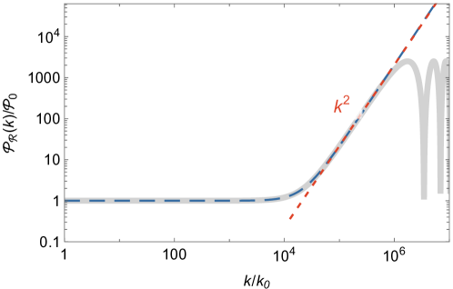
Figure 2: The evolution of the power spectrum as a function of wave number $k$. The solid-gray and dashed-blue lines represent the numerical and approximate results, respectively. The dashed-red line indicates the $k^{2}$ growth.

III Growth behavior of power spectrum when both the sound speed and the slow-roll parameter $\eta$ are changed suddenly

We have known that the enhancement of the power spectrum can be realized by decreasing the sound speed $c_{s}$ or reducing the slow-roll parameter $\epsilon$. In the following, we will study the growth of the power spectrum when both $\epsilon$ and $c_{s}$ are suppressed. For simplicity, we will consider that the sound speed changes suddenly from $1$ to a constant much less than one, and the slow-roll parameter $\eta$ suddenly from a constant near zero to a negative constant. A negative $\eta$ will lead to the decrease of $\epsilon$ since $\epsilon\propto\tau^{-\eta}$. We first consider the case that the variations of $c_{s}$ and $\eta$ occur simultaneously.

III.1 Simultaneous changes of sound speed and slow-roll parameter $\eta$

The scenario considered in this subsection is shown in Fig. 3. Initially, the Universe undergoes a standard slow-roll inflation, in which $c_{s}=1$, $\epsilon\simeq\epsilon_{0}\ll 1$ and $\eta\sim 0$. At time $\tau_{1}$, the sound speed $c_{s}$ and the slow-roll parameter $\eta$ change suddenly from $1$ and $\sim 0$ to a small value $c_{s_{1}}$ and a negative constant $\eta_{1}$, respectively. Thus, during the second phase, the slow-roll parameter $\epsilon$ decays as $\epsilon(\tau)=\epsilon_{0}(\tau/\tau_{1})^{-\eta_{1}}$ and the sound speed is a small constant $c_{s_{1}}$.

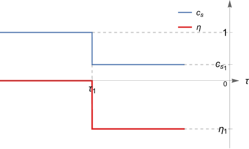
Figure 3: The slow-roll parameter $\eta$ (red line) and the sound speed $c_{s}$ (blue line) vary simultaneously at $\tau_{1}$.

From Eq. (6), we obtain the general solution of the curvature perturbations

$$\overline{\mathcal{R}}^{(1)}_{k}(\tau)=-\frac{c_{s_{1}}H\tau_{1}^{-\frac{\eta_{1}}{2}}\tau^{\frac{3+\eta_{1}}{2}}}{\sqrt{2\epsilon_{0}}}\left[\alpha_{2}H_{\nu}^{(1)}(c_{s_{1}}k\tau)+\beta_{2}H_{\nu}^{(2)}(c_{s_{1}}k\tau)\right]\;$$ (17)

in the second phase, where $\alpha_{2}$ and $\beta_{2}$ are two constants, and $\nu=(3+\eta_{1})/2$. Matching $\mathcal{R}^{(0)}_{k}$ and $\overline{\mathcal{R}}^{(1)}_{k}$ at $\tau=\tau_{1}$ by using the improved junction conditions, $\mathcal{R}^{(0)}_{k}(\tau_{1})=\overline{\mathcal{R}}^{(1)}_{k}(\tau_{1})$ and $A_{0}\mathcal{R}^{\prime(0)}_{k}(\tau_{1})=A_{1}\overline{\mathcal{R}}^{\prime(1)}_{k}(\tau_{1})$, one can achieve that

$$\alpha_{2} = \frac{\pi e^{-ik\tau_{1}}}{4\sqrt{2c_{s_{1}}^{2}\tau_{1}^{3}k^{3}}}\bigg{[}\left(\left(3+\eta_{1}\right)\left(1+ik\tau_{1}\right)-(c_{s_{1}}k\tau_{1})^{2}\right)H_{\nu}^{(2)}(c_{s_{1}}k\tau_{1})$$

$$\qquad\qquad\qquad-c_{s_{1}}k\tau_{1}\left(1+ik\tau_{1}\right)H_{\nu+1}^{(2)}(c_{s_{1}}k\tau_{1})\bigg{]}\;,$$

and

$$\beta_{2} = -\frac{\pi e^{-ik\tau_{1}}}{4\sqrt{2c_{s_{1}}^{2}\tau_{1}^{3}k^{3}}}\bigg{[}\left(\left(3+\eta_{1}\right)\left(1+ik\tau_{1}\right)-(c_{s_{1}}k\tau_{1})^{2}\right)H_{\nu}^{(1)}(c_{s_{1}}k\tau_{1})$$

$$\qquad\qquad\qquad-c_{s_{1}}k\tau_{1}\left(1+ik\tau_{1}\right)H_{\nu+1}^{(1)}(c_{s_{1}}k\tau_{1})\bigg{]}\;.$$

Substituting $\alpha_{2}$ and $\beta_{2}$ into Eq. (17) gives the expression of the curvature perturbations during the second phase. Expanding this expression in the infrared limit ($-c_{s_{1}}k\tau\rightarrow 0$ and $-c_{s_{1}}k\tau_{1}\rightarrow 0$), we arrive at

$$\overline{\mathcal{R}}^{(1)}_{k}(\tau) = \frac{iHe^{-ik\tau_{1}}}{2\sqrt{\epsilon_{0}k^{3}}}-\frac{H\tau_{1}e^{-ik\tau_{1}}}{2\sqrt{\epsilon_{0}k}}-\left(\frac{3ic_{s_{1}}^{2}H\tau_{1}^{2}e^{-ik\tau_{1}}}{4\sqrt{\epsilon_{0}}(3+\eta_{1})}+\frac{ic_{s_{1}}^{2}H\eta_{1}\left(-\tau_{1}\right)^{-1-\eta_{1}}e^{-ik\tau_{1}}}{2\sqrt{\epsilon_{0}}(1+\eta_{1})(3+\eta_{1})}(-\tau)^{3+\eta_{1}}\right)k^{1/2}$$ (18)

$$+ \left(\frac{c_{s_{1}}^{2}H\tau_{1}^{3}e^{-ik\tau_{1}}}{4\sqrt{\epsilon_{0}}(3+\eta_{1})}-\frac{c_{s_{1}}^{2}He^{-ik\tau_{1}}}{2\sqrt{\epsilon_{0}}(1+\eta_{1})(3+\eta_{1})\left(-\tau_{1}\right)^{\eta_{1}}}(-\tau)^{3+\eta_{1}}\right)k^{3/2}$$

$$+ \dots\;.$$

It is easy to see that the solution contains a time-independent part and a time-dependent one, which will decay with time when $\eta_{1}>-3$, and grow when $\eta_{1}<-3$.

Now, we assume that the second phase lasts for $N_{2}$ number of e-folds, which means that $\tau_{2}=\tau_{1}e^{-N_{2}}$ if this phase ends at $\tau=\tau_{2}$. The power spectrum of the curvature perturbations can be obtained from Eq. (18), which takes the form

$$\dfrac{\mathcal{P}_{\overline{\mathcal{R}}^{(2)}_{k}}}{\mathcal{P}_{0}} \simeq 1+\left(1+\frac{2c_{s_{1}}^{2}\eta_{1}}{(1+\eta_{1})(3+\eta_{1})}e^{-\left(3+\eta_{1}\right)N_{2}}\right)\tau_{1}^{2}k^{2}$$

$$- \left(\begin{split}&\frac{1}{3+\eta_{1}}+\frac{2}{(1+\eta_{1})(3+\eta_{1})}e^{-\left(3+\eta_{1}\right)N_{2}}-\frac{c_{s_{1}}^{2}\eta_{1}^{2}}{(1+\eta_{1})^{2}(3+\eta_{1})^{2}}e^{-2\left(3+\eta_{1}\right)N_{2}}\end{split}\right)c_{s_{1}}^{2}\tau_{1}^{4}k^{4}$$

$$+ \left(\begin{split}&\frac{1}{4(3+\eta_{1})^{2}}+\frac{1}{(1+\eta_{1})(3+\eta_{1})^{2}}e^{-\left(3+\eta_{1}\right)N_{2}}+\frac{1}{(1+\eta_{1})^{2}(3+\eta_{1})^{2}}e^{-2\left(3+\eta_{1}\right)N_{2}}\end{split}\right)c_{s_{1}}^{4}\tau_{1}^{6}k^{6}\;.$$

Here we have kept the $k^{6}$ term in Eq. (III.1) since the $k^{6}$ growth may occur under certain conditions. We need to compare the $k^{n}$ term with the $k^{n-2}$ one to determine whether a $k^{n}$ growth will appear. We set $k_{1}$, $k_{2}$, and $k_{3}$ to denote the wave number at which the scale-invariant term becomes comparable with the $k^{2}$ term, the $k^{2}$ term becomes comparable with the $k^{4}$ term, and the $k^{4}$ term becomes comparable with the $k^{6}$ term, respectively.

Let us first study the $\eta_{1}>-3$ case, which means that there are no growing terms in the solution of the curvature perturbations and all time-dependent terms in Eq. (18) decay with the cosmic expansion. Thus, all terms containing $N_{2}$ in Eq. (III.1) can be neglected. Then, we find that

$$k_{1}\simeq-\frac{1}{\tau_{1}}=c_{s_{1}}k_{c}\;,$$ (20)

and

$$k_{2}\simeq-\frac{\sqrt{3+\eta_{1}}}{c_{s_{1}}\tau_{1}}=\sqrt{3+\eta_{1}}k_{c}\;.$$ (21)

The condition $k_{2}\ll k_{c}$ for a $k^{4}$ growth requires that $\sqrt{3+\eta_{1}}\ll 1$. This is hard to satisfy since $\eta_{1}$ must be fine-tuned to be very close to $-3$. Thus, usually the highest growth of the power spectrum can only reach $k^{2}$. Furthermore, since the power spectrum only has the $k^{2}$ growth, the dip phenomenon does not appear. These characters can be found clearly in Fig. 4, where the power spectrums from numerical and approximate analyses are plotted in the $\eta_{1}=-2$ case.

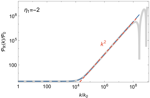
Figure 4: The power spectrum in the $\eta_{1}=-2$ case. The gray-solid and blue-dashed lines represent the numerical and approximate results, respectively. The dashed-red line indicates the $k^{2}$ growth.

Table 1: The predominant terms of $k^{n}$ in three different situations.

	$c_{s_{1}}^{2}e^{-(3+\eta_{1})N_{2}}\ll 1$	$c_{s_{1}}^{2}e^{-(3+\eta_{1})N_{2}}=1$	$c_{s_{1}}^{2}e^{-(3+\eta_{1})N_{2}}\gg 1$
$\tau_{1}^{2}k^{2}$	$1$	$1+\frac{2\eta_{1}}{(1+\eta_{1})(3+\eta_{1})}$	$\frac{2c_{s_{1}}^{2}\eta_{1}e^{-(3+\eta_{1})N_{2}}}{(1+\eta_{1})(3+\eta_{1})}$
$c_{s_{1}}^{2}\tau_{1}^{4}k^{4}$	$-\frac{2e^{-\left(3+\eta_{1}\right)N_{2}}}{(1+\eta_{1})(3+\eta_{1})}$	$-\frac{(\eta_{1}^{2}+8\eta_{1}+6)e^{-\left(3+\eta_{1}\right)N_{2}}}{(1+\eta_{1})^{2}(3+\eta_{1})^{2}}$	$\frac{c_{s_{1}}^{2}\eta_{1}^{2}e^{-2\left(3+\eta_{1}\right)N_{2}}}{(1+\eta_{1})^{2}(3+\eta_{1})^{2}}$
$c_{s_{1}}^{4}\tau_{1}^{6}k^{6}$	$\frac{e^{-2\left(3+\eta_{1}\right)N_{2}}}{(1+\eta_{1})^{2}(3+\eta_{1})^{2}}$	$\frac{e^{-2\left(3+\eta_{1}\right)N_{2}}}{(1+\eta_{1})^{2}(3+\eta_{1})^{2}}$	$\frac{e^{-2\left(3+\eta_{1}\right)N_{2}}}{(1+\eta_{1})^{2}(3+\eta_{1})^{2}}$

When $\eta_{1}<-3$, since the coefficient of the $k^{n}$ term is very tedious, we only consider three special cases ($c_{s_{1}}^{2}e^{-(3+\eta_{1})N_{2}}\ll 1$, $c_{s_{1}}^{2}e^{-(3+\eta_{1})N_{2}}=1$ and $c_{s_{1}}^{2}e^{-(3+\eta_{1})N_{2}}\gg 1$), as shown in Table 1 in which the predominant terms of $k^{n}$ are given, to investigate analytically the growth of the power spectrum. In the case of $c_{s_{1}}^{2}e^{-(3+\eta_{1})N_{2}}\ll 1$, we find that

$$k_{1} \simeq -\frac{1}{\tau_{1}}=c_{s_{1}}k_{c}\;,$$

$$k_{2} \simeq -\frac{\sqrt{(1+\eta_{1})(3+\eta_{1})}}{\sqrt{2}c_{s_{1}}\tau_{1}}e^{\frac{(3+\eta_{1})N_{2}}{2}}=\frac{\sqrt{(1+\eta_{1})(3+\eta_{1})}}{\sqrt{2}}e^{\frac{(3+\eta_{1})N_{2}}{2}}k_{c}\;,$$

$$k_{3} \simeq -\frac{\sqrt{2(1+\eta_{1})(3+\eta_{1})}}{c_{s_{1}}\tau_{1}}e^{\frac{(3+\eta_{1})N_{2}}{2}}=\sqrt{2(1+\eta_{1})(3+\eta_{1})}e^{\frac{(3+\eta_{1})N_{2}}{2}}k_{c}\;.$$ (22)

Apparently, the condition $k_{3}<k_{c}$ is easy to be satisfied since $\eta_{1}<-3$. Thus the power spectrum can have a $k^{6}$ growth. Since the coefficient of the $k_{4}$ term is negative, the power spectrum has a dip preceding the $k^{6}$ growth.

When $c_{s_{1}}^{2}e^{-(3+\eta_{1})N_{2}}=1$, we have

$$k_{1} \simeq \sqrt{\frac{\eta_{1}^{2}+4\eta_{1}+3}{(\eta_{1}^{2}+6\eta_{1}+3)}}c_{s_{1}}k_{c}\;,$$

$$k_{2} \simeq \sqrt{\frac{(\eta_{1}^{2}+4\eta_{1}+3)(\eta_{1}^{2}+6\eta_{1}+3)}{(\eta_{1}^{2}+8\eta_{1}+6)}}c_{s_{1}}k_{c}\;,$$

$$k_{3} \simeq \sqrt{\eta_{1}^{2}+8\eta_{1}+6}~{}c_{s_{1}}k_{c}\;.$$ (23)

We find that $k_{1}\simeq k_{2}\simeq k_{3}<k_{c}$, which means that the power spectrum will go directly to the $k^{6}$ growth after the scale-invariant spectrum.

In the case of $c_{s_{1}}^{2}e^{-(3+\eta_{1})N_{2}}\gg 1$, one can obtain

$$k_{1} \simeq \frac{\sqrt{(1+\eta_{1})(3+\eta_{1})}}{\sqrt{-2\eta_{1}}}e^{\frac{1}{2}(3+\eta_{1})N_{2}}k_{c}\;,$$

$$k_{2} \simeq \frac{\sqrt{(1+\eta_{1})(3+\eta_{1})}}{\sqrt{-\eta_{1}}}e^{\frac{1}{2}(3+\eta_{1})N_{2}}k_{c}\;,$$

$$k_{3} \simeq |\eta_{1}|c_{s_{1}}k_{c}\;.$$ (24)

Since $k_{2}\ll k_{c}$, the power spectrum will grow with $k^{4}$ when the scales become smaller than the CMB one. It eventually goes into $k^{6}$ growth due to $k_{3}<k_{c}$. A negative $\eta_{1}$ leads to a negative coefficient of the $k^{2}$ term, which indicates that the power spectrum has a dip preceding the $k^{4}$ growth. These characters can be seen in Fig. 5, where the numerical (gray -solid lines) and approximate (blue-dashed lines) results of the power spectrum with $\eta_{1}=-4,-5,-6$ are plotted. One can see that the approximate results are consistent with the numerical ones.

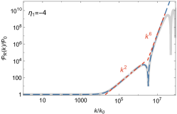
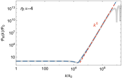
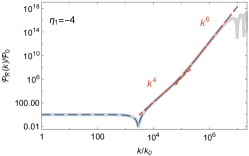
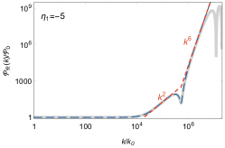
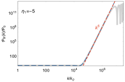
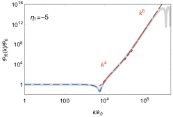
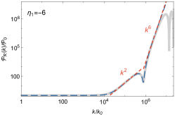
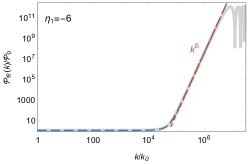
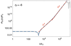
Figure 5: The power spectrums in the $\eta_{1}=-4$, $-5$, and $-6$ cases. The gray-solid and blue-dashed lines represent the numerical and approximate results, respectively. The first, middle and last columns correspond to the $c_{s_{1}}^{2}e^{-(3+\eta_{1})N_{2}}\ll 1$, $c_{s_{1}}^{2}e^{-(3+\eta_{1})N_{2}}=1$, and $c_{s_{1}}^{2}e^{-(3+\eta_{1})N_{2}}\gg 1$ cases, respectively.

Moreover, Eq. (18) is clearly inapplicable for the cases of $\eta_{1}=-1$ and $\eta_{1}=-3$ due to the appearance of singularity. These two cases need to be treated separately.

• $\eta_{1}=-1$

We find that in the infrared limit, the solution of the curvature perturbations [Eq. (17)] has the form

$$\overline{\mathcal{R}}^{(1)}_{k}(\tau)=\frac{iHe^{-ik\tau_{1}}}{2\sqrt{\epsilon_{0}k^{3}}}-\frac{H\tau_{1}e^{-ik\tau_{1}}}{2\sqrt{\epsilon_{0}k}}-\dfrac{ic_{s_{1}}^{2}Hk^{1/2}e^{-ik\tau_{1}}}{8\sqrt{\epsilon_{0}}}\left[3\tau_{1}^{2}-(-\tau)^{2}\right]+\dots\;.$$ (25)

The solution of the curvature perturbations consists of the constant part and the decaying one, which is similar to the solution in the case of $\eta_{1}>-3$. The power spectrum of the curvature perturbations has the form

$$\dfrac{\mathcal{P}_{\overline{\mathcal{R}}^{(1)}_{k}}}{\mathcal{P}_{0}}\simeq 1+\tau_{1}^{2}k^{2}+\frac{9}{16}c_{s_{1}}^{4}\tau_{1}^{4}k^{4}\;.$$ (26)

We can see that the $k^{2}$ and $k^{4}$ terms become comparable at

$$k_{2}\approx-\frac{4}{3c_{s_{1}}^{2}\tau_{1}}=\frac{4}{3c_{s_{1}}}k_{c}\;.$$ (27)

Since $k_{2}>k_{c}$, the power spectrum has no $k^{4}$ growth. The corresponding numerical and approximate results of the power spectrum are shown in Fig. 6. Apparently at the small scales the power spectrum grows with a $k^{2}$ slope.

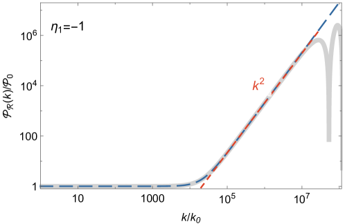
Figure 6: The power spectrum in the $\eta_{1}=-1$ case .The gray-solid and blue-dashed lines represent the numerical and approximate results, respectively. The dashed-red line indicates the $k^{2}$ growth.

• $\eta_{1}=-3$

In the infrared limit, Eq. (17) can be simplified to be

$$\overline{\mathcal{R}}^{(1)}_{k}(\tau) = \frac{iHe^{-ik\tau_{1}}}{2\sqrt{\epsilon_{0}k^{3}}}-\frac{H\tau_{1}e^{-ik\tau_{1}}}{2\sqrt{\epsilon_{0}k}}+\dfrac{ic_{s_{1}}^{2}H\tau_{1}^{2}k^{1/2}e^{-ik\tau_{1}}}{8\sqrt{\epsilon_{0}}}\left[1+6\log\left(\dfrac{\tau}{\tau_{1}}\right)\right]$$ (28)

$$- \dfrac{ic_{s_{1}}^{2}H\tau_{1}^{3}k^{3/2}e^{-ik\tau_{1}}}{8\sqrt{\epsilon_{0}}}\left[1+2\log\left(\dfrac{\tau}{\tau_{1}}\right)\right]+\dots\;.$$

The solution for the curvature perturbation consists of the constant term and the logarithmically growing one. This characteristic is different from the power-law growth in the $\eta_{1}<-3$ case. Thus, we obtain that the power spectrum has the expression

$$\dfrac{\mathcal{P}_{\overline{\mathcal{R}}^{(1)}_{k}}}{\mathcal{P}_{0}} \simeq 1+\frac{1}{2}\left(2-c_{s_{1}}^{2}\left(6N_{2}-1\right)\right)\tau_{1}^{2}k^{2}+\frac{1}{16}c_{s_{1}}^{2}\left(8+c_{s_{1}}^{2}\left(6N_{2}-1\right)^{2}-16N_{2}\right)\tau_{1}^{4}k^{4}$$ (29)

$$+ \frac{1}{16}c_{s_{1}}^{4}\left(2N_{2}-1\right)^{2}\tau_{1}^{6}k^{6}\;.$$

Since the maximum value of $N_{2}$ is about $30-40$ and $c_{s_{1}}\sim\mathcal{O}(10^{-4})$, $N_{2}c_{s_{1}}^{2}$ is significantly less than 1. Therefore, the expression of the power spectrum given in Eq. (29) can be simplified to be

$$\dfrac{\mathcal{P}_{\overline{\mathcal{R}}^{(1)}_{k}}}{\mathcal{P}_{0}}\simeq 1+\tau_{1}^{2}k^{2}+\frac{1}{2}(1-2N_{2})c_{s_{1}}^{2}\tau_{1}^{4}k^{4}+\frac{1}{16}(2N_{2}-1)^{2}c_{s_{1}}^{4}\tau_{1}^{6}k^{6}\;.$$ (30)

From the above expression, we obtain

$$k_{1} \simeq c_{s_{1}}k_{c}\;,$$

$$k_{2} \simeq \frac{1}{\sqrt{N_{2}-1/2}}k_{c}\;,$$

$$k_{3} \simeq \frac{2}{\sqrt{N_{2}-1/2}}k_{c}\;.$$ (31)

Obviously, $k_{1}\ll k_{c}$ and $k_{2}\approx k_{3}$, which are less than $k_{c}$ if $N_{2}>9/2$. Thus, the power spectrum will have an era with a $k^{2}$ growth and eventually with a $k^{6}$ one at scales smaller than the CMB one when $N_{2}>9/2$. Since the coefficient of the $k^{4}$ term is negative, there is a dip preceding the $k^{6}$ growth. These characters can be seen clearly in Fig. 7.

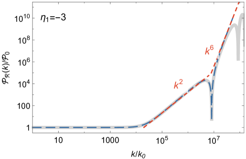
Figure 7: The power spectrum in the $\eta_{1}=-3$ case. The gray-solid and blue-dashed lines represent the numerical and approximate results, respectively.

III.2 Changes of sound speed previous to slow-roll parameter $\eta$

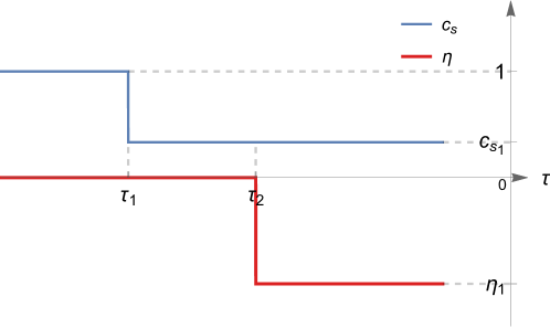
Figure 8: The sound speed $c_{s}$ (blue line) varies at $\tau_{1}$, and the slow-roll parameter $\eta$ (red line) changes at $\tau_{2}$ $(|\tau_{2}|<|\tau_{1}|$).

The simultaneous change of $c_{s}$ and $\eta$ is a harsh requirement. In the following, we abandon it, and first consider that the change of the sound speed is followed by that of $\eta$. We assume that the sound speed changes suddenly from $1$ to a small constant $c_{s_{1}}$ at time $\tau_{1}$, and $\eta$ varies from $\sim 0$ to a negative constant $\eta_{1}$ at $\tau_{2}$ ($|\tau_{2}|<|\tau_{1}|$), as is shown in Fig. 8. The $|\tau|>|\tau_{1}|$ era, which represents the first phase, is the standard slow-roll inflation. In the second phase ($|\tau_{2}|<|\tau|<|\tau_{1}|$), the sound speed of the curvature perturbations is a small value $c_{s_{1}}$. When $|\tau|<|\tau_{2}|$, which corresponds to the third phase, the slow-roll parameter $\epsilon$ decreases with the power-law: $\epsilon(\tau)=\epsilon_{0}(\tau/\tau_{2})^{-\eta_{1}}$ and the sound speed keeps the small value $c_{s_{1}}$.

When $|\tau|>|\tau_{1}|$, the solution of $\mathcal{R}_{k}^{(0)}$ is given in Eq. (7). In the second phase, the solution of the curvature perturbations has the form

$$\widetilde{\mathcal{R}}^{(1)}_{k}(\tau)=\frac{ic_{s_{1}}H\left(-\tau\right)^{3/2}}{\sqrt{2\epsilon_{0}}}\left[\alpha_{3}H_{3/2}^{(1)}(c_{s_{1}}k\tau)+\beta_{3}H_{3/2}^{(2)}(c_{s_{1}}k\tau)\right]\;,$$ (32)

where $\alpha_{3}$ and $\beta_{3}$ are two constants. Using the matching condition: $\mathcal{R}^{(0)}_{k}(\tau_{1})=\widetilde{\mathcal{R}}^{(1)}_{k}(\tau_{1})$ and $A_{0}\mathcal{R}^{\prime(0)}_{k}(\tau_{1})=A_{1}\widetilde{\mathcal{R}}^{\prime(1)}_{k}(\tau_{1})$, one can obtain that

$$\alpha_{3} = -\frac{\left(1-c_{s_{1}}\right)\sqrt{\pi}e^{-i\left(1+c_{s_{1}}\right)k\tau_{1}}}{4\sqrt{c_{s_{1}}}},$$

$$\beta_{3} = -\frac{\left(1+c_{s_{1}}\right)\sqrt{\pi}e^{-i\left(1-c_{s_{1}}\right)k\tau_{1}}}{4\sqrt{c_{s_{1}}}}\;.$$ (33)

If $|\tau|<|\tau_{2}|$, the solution of the curvature perturbations becomes

$$\widetilde{\mathcal{R}}^{(2)}_{k}(\tau)=-\frac{c_{s_{1}}H\tau_{2}^{-\frac{\eta_{1}}{2}}\tau^{\frac{3+\eta_{1}}{2}}}{\sqrt{2\epsilon_{0}}}\left[\alpha_{4}H_{\nu}^{(1)}(c_{s_{1}}k\tau)+\beta_{4}H_{\nu}^{(2)}(c_{s_{1}}k\tau)\right],$$ (34)

where $\alpha_{4}$ and $\beta_{4}$ are two constants and $\nu=(3+\eta_{1})/2$. Using the matching condition: $\widetilde{\mathcal{R}}^{(1)}_{k}(\tau_{2})=\widetilde{\mathcal{R}}^{(2)}_{k}(\tau_{2})$ and $\widetilde{\mathcal{R}}^{\prime(1)}_{k}(\tau_{2})=\widetilde{\mathcal{R}}^{\prime(2)}_{k}(\tau_{2})$, one finds

$$\alpha_{4} = \frac{i\pi^{3/2}c_{s_{1}}^{1/2}\tau_{2}k}{16}e^{-i(1+c_{s_{1}})k\tau_{1}}\left[~{}\xi H_{\frac{3+\eta_{1}}{2}}^{(2)}(c_{s_{1}}k\tau_{2})-\lambda H_{\frac{1+\eta_{1}}{2}}^{(2)}(c_{s_{1}}k\tau_{2})\right],$$ (35)

$$\beta_{4} = -\frac{i\pi^{3/2}c_{s_{1}}^{1/2}\tau_{2}k}{16}e^{-i(1+c_{s_{1}})k\tau_{1}}\left[~{}\xi H_{\frac{3+\eta_{1}}{2}}^{(1)}(c_{s_{1}}k\tau_{2})-\lambda H_{\frac{1+\eta_{1}}{2}}^{(1)}(c_{s_{1}}k\tau_{2})\right]\;,$$ (36)

where

$$\xi =(1-c_{s_{1}})H_{\frac{1}{2}}^{(1)}(c_{s_{1}}k\tau_{2})+(1+c_{s_{1}})e^{2ic_{s_{1}}k\tau_{1}}H_{\frac{1}{2}}^{(2)}(c_{s_{1}}k\tau_{2})\;,$$

$$\lambda =(1-c_{s_{1}})H_{\frac{3}{2}}^{(1)}(c_{s_{1}}k\tau_{2})+(1+c_{s_{1}})e^{2ic_{s_{1}}k\tau_{1}}H_{\frac{3}{2}}^{(2)}(c_{s_{1}}k\tau_{2})\;.$$ (37)

In the infrared region ($-c_{s_{1}}k\tau\rightarrow 0$, $-c_{s_{1}}k\tau_{1}\rightarrow 0$ and $-c_{s_{1}}k\tau_{2}\rightarrow 0$ ), we obtain that

$$\widetilde{\mathcal{R}}^{(2)}_{k}(\tau) = \frac{iHe^{-ik\tau_{1}}}{2\sqrt{\epsilon_{0}k^{3}}}-\frac{H\tau_{1}e^{-ik\tau_{1}}}{2\sqrt{\epsilon_{0}k}}$$ (38)

$$- \left(\frac{ic_{s_{1}}^{2}H\left((3+\eta_{1})\tau_{1}^{2}-\eta_{1}\tau_{2}^{2}\right)e^{-ik\tau_{1}}}{4\sqrt{\epsilon_{0}}(3+\eta_{1})}+\frac{ic_{s_{1}}^{2}H\eta_{1}\tau_{2}^{-1-\eta_{1}}e^{i\pi\eta_{1}-ik\tau_{1}}}{2\sqrt{\epsilon_{0}}(1+\eta_{1})(3+\eta_{1})}(-\tau)^{3+\eta_{1}}\right)k^{1/2}$$

$$+ \left(\begin{split}&\frac{c_{s_{1}}^{2}H\left((3+\eta_{1})\tau_{1}^{3}-3\eta_{1}\tau_{1}\tau_{2}^{2}+2\eta_{1}\tau_{2}^{3}\right)e^{-ik\tau_{1}}}{12\sqrt{\epsilon_{0}}(3+\eta_{1})}\\ +&\frac{c_{s_{1}}^{2}H\left(\eta_{1}\tau_{1}-\tau_{2}-\eta_{1}\tau_{2}\right)\tau_{2}^{-1-\eta_{1}}e^{i\pi\eta_{1}-ik\tau_{1}}}{2\sqrt{\epsilon_{0}}(1+\eta_{1})(3+\eta_{1})}(-\tau)^{3+\eta_{1}}\end{split}\right)k^{3/2}$$

$$+ \dots\;.$$

Clearly, the solution given in Eq. (38) contains a time-independent part and a time-dependent one, which will grow with time when $\eta_{1}<-3$.

Using $N_{2}$ and $N_{3}$ to denote the number of $e$-folds during the second and third phases, respectively, i.e. $\tau_{2}=\tau_{1}e^{-N_{2}}$ and $\tau=\tau_{1}e^{-N_{2}-N_{3}}$, we obtain, from Eq. (38), the expression of the power spectrum of the curvature perturbations

$$\dfrac{\mathcal{P}_{\widetilde{\mathcal{R}}^{(2)}_{k}}}{\mathcal{P}_{0}} \simeq 1+\left(1-c_{s_{1}}^{2}+\frac{c_{s_{1}}^{2}\eta_{1}}{3+\eta_{1}}e^{-2N_{2}}+\frac{2c_{s_{1}}^{2}\eta_{1}}{(1+\eta_{1})(3+\eta_{1})}e^{-2N_{2}-\left(3+\eta_{1}\right)N_{3}}\right)\tau_{1}^{2}k^{2}$$ (39)

$$- \left(\begin{split}&\frac{1}{3}+\frac{2\eta_{1}e^{-3N_{2}}}{9+3\eta_{1}}-\frac{3\eta_{1}e^{-2N_{2}}}{9+3\eta_{1}}+\frac{2+2\eta_{1}-2\eta_{1}e^{N_{2}}}{(1+\eta_{1})(3+\eta_{1})}e^{-3N_{2}-\left(3+\eta_{1}\right)N_{3}}\\ -&c_{s_{1}}^{2}\left(\frac{1}{2}-\frac{\eta_{1}}{6+2\eta_{1}}e^{-2N_{2}}-\frac{\eta_{1}}{(1+\eta_{1})(3+\eta_{1})}e^{-2N_{2}-\left(3+\eta_{1}\right)N_{3}}\right)^{2}\end{split}\right)c_{s_{1}}^{2}\tau_{1}^{4}k^{4}$$

$$+ \left(\frac{1}{6}+\frac{\eta_{1}e^{-3N_{2}}}{9+3\eta_{1}}-\frac{\eta_{1}e^{-2N_{2}}}{6+2\eta_{1}}+\frac{1+\eta_{1}-\eta_{1}e^{N_{2}}}{(1+\eta_{1})(3+\eta_{1})}e^{-3N_{2}-\left(3+\eta_{1}\right)N_{3}}\right)^{2}c_{s_{1}}^{4}\tau_{1}^{6}k^{6}\;.$$

We first study the $\eta_{1}>-3$ case, which means that there are no growing terms in the solution of the curvature perturbations and all time-dependent terms in Eq. (38) decay with the cosmic expansion. Thus, all terms containing $N_{2}$ and $N_{3}$ in Eq. (39) can be neglected and the power spectrum can be simplified as

$$\dfrac{\mathcal{P}_{\widetilde{\mathcal{R}}^{(2)}_{k}}}{\mathcal{P}_{0}} \simeq 1+\tau_{1}^{2}k^{2}-\frac{1}{3}c_{s_{1}}^{2}\tau_{1}^{4}k^{4}+\frac{1}{36}c_{s_{1}}^{4}\tau_{1}^{6}k^{6}\;.$$ (40)

It can be found that the wave numbers at which the scale-invariant term is comparable to the $k^{2}$ term and the $k^{2}$ term is comparable to $k^{4}$ one happen, respectively, at

$$k_{1} \simeq c_{s_{1}}k_{c}\;,$$

$$k_{2} \simeq \sqrt{3}k_{c}\;.$$ (41)

The power spectrum has a growth rate of $k^{2}$ since $k_{2}>k_{c}$. These results can be found clearly in Fig. 9, where the evolutions of the power spectrum from numerical and approximate analyses are plotted in the $\eta_{1}=-2$ case. At the CMB scale, the power spectrum is scale invariant which is consistent with the CMB observations. At scales smaller than the CMB scale, the power spectrum becomes scale-dependent with a $k^{2}$ growth.

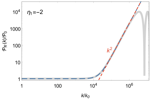
Figure 9: The power spectrum in the $\eta_{1}=-2$ case. The gray-solid and blue-dashed lines represent the numerical and approximate results, respectively. The red-dashed line indicates the $k^{2}$ growth.

When $\eta_{1}<-3$, since the coefficient of $k^{n}$ is very tedious, we only consider three special cases ($N_{2}\gg N_{3}$, $N_{2}\ll N_{3}$, and $N_{2}=N_{3}$) to investigate analytically the growth of the power spectrum.

First of all, when $N_{2}\gg N_{3}$, all terms containing $N_{2}$ in Eq. (39) can be neglected. Thus, the dominant term of $k^{n}$ is the same as the one in the case of $\eta_{1}>-3$. Therefore, the evolution of the power spectrum is the same as in the case of $\eta_{1}>-3$, and only has the $k^{2}$ growth.

When $N_{2}=N_{3}$, the expression for the power spectrum given in Eq. (39) can be simplified to be

$$\frac{\mathcal{P}_{\widetilde{\mathcal{R}}^{(2)}_{k}}}{\mathcal{P}_{0}} \simeq 1+\tau_{1}^{2}k^{2}-\left(\frac{1}{3}-\frac{2\eta_{1}}{(1+\eta_{1})(3+\eta_{1})}e^{-\left(5+\eta_{1}\right)N_{3}}\right)c_{s_{1}}^{2}\tau_{1}^{4}k^{4}$$ (42)

$$+ \left(\frac{1}{36}-\frac{\eta_{1}}{3(1+\eta_{1})(3+\eta_{1})}e^{-\left(5+\eta_{1}\right)N_{3}}+\frac{\eta_{1}^{2}}{(1+\eta_{1})^{2}(3+\eta_{1})^{2}}e^{-2\left(5+\eta_{1}\right)N_{3}}\right)c_{s_{1}}^{4}\tau_{1}^{6}k^{6}\;.$$

Since different values of $\eta_{1}$ will give different results, we will discuss this situation by considering following different cases:

$$\frac{\mathcal{P}_{\widetilde{\mathcal{R}}^{(2)}_{k}}}{\mathcal{P}_{0}}\simeq\left\{\begin{array}[]{ll}1+\tau_{1}^{2}k^{2}-\dfrac{1}{3}c_{s_{1}}^{2}\tau_{1}^{4}k^{4}+\dfrac{1}{36}c_{s_{1}}^{4}\tau_{1}^{6}k^{6}&-5<\eta_{1}<-3\vspace{0.4cm}\\ 1+\tau_{1}^{2}k^{2}-\dfrac{19}{12}c_{s_{1}}^{2}\tau_{1}^{4}k^{4}+\dfrac{361}{576}c_{s_{1}}^{4}\tau_{1}^{6}k^{6}&~{}~{}~{}~{}\eta_{1}=-5\vspace{0.4cm}\\ 1+\tau_{1}^{2}k^{2}+\dfrac{2\eta_{1}e^{-\left(5+\eta_{1}\right)N_{3}}}{(1+\eta_{1})(3+\eta_{1})}c_{s_{1}}^{2}\tau_{1}^{4}k^{4}+\dfrac{\eta_{1}^{2}e^{-2\left(5+\eta_{1}\right)N_{3}}}{(1+\eta_{1})^{2}(3+\eta_{1})^{2}}c_{s_{1}}^{4}\tau_{1}^{6}k^{6}&~{}~{}~{}~{}\eta_{1}<-5\ .\\ \end{array}\right.$$

When $-5\leq\eta_{1}<-3$, we find that $k_{2}\simeq k_{c}$, which means that the power spectrum only has the $k^{2}$ growth. In the $\eta_{1}<-5$ case, we obtain

$$k_{1} \simeq c_{s_{1}}k_{c}\;,$$

$$k_{2} \simeq \frac{\sqrt{(1+\eta_{1})(3+\eta_{1})}}{\sqrt{-2\eta_{1}}}e^{\frac{1}{2}(5+\eta_{1})N_{3}}k_{c}\;,$$

$$k_{3} \simeq \frac{\sqrt{2(1+\eta_{1})(3+\eta_{1})}}{\sqrt{-\eta_{1}}}e^{\frac{1}{2}(5+\eta_{1})N_{3}}k_{c}\;.$$ (46)

Apparently, $k_{3}$ is less than $k_{c}$ if $\frac{\sqrt{2(1+\eta_{1})(3+\eta_{1})}}{\sqrt{-\eta_{1}}}e^{\frac{1}{2}(5+\eta_{1})N_{3}}\ll 1$, which can be realized easily since $\eta_{1}<-5$. Thus, the power spectrum can have the $k^{6}$ growth. Since there is a negative coefficient in the $k^{4}$ term, the power spectrum has a dip preceding the $k^{6}$ growth. In Fig. 10, the power spectrums in the cases of $\eta_{1}=-4,-5$ and $-6$ for the $N_{2}\gg N_{3}$ and $N_{2}=N_{3}$ cases are plotted. We can see that when $N_{2}\gg N_{3}$, the highest growth slope of the power spectrum is $k^{2}$. In the case of $N_{2}=N_{3}$, the highest growth rate for $\eta_{1}=-4$ and $-5$ is still $k^{2}$, while for $\eta_{1}=-6$, the highest growth rate can reach up to $k^{6}$.

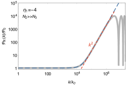
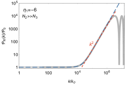
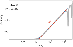
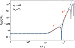
Figure 10: The power spectrums in the $\eta_{1}=-4$, $-5$ and $-6$ cases. The gray-solid and blue-dashed lines represent the numerical and approximate results, respectively.

When $N_{2}\ll N_{3}$, the power spectrum can be approximated as

$$\frac{\mathcal{P}_{\widetilde{\mathcal{R}}^{(2)}_{k}}}{\mathcal{P}_{0}} \simeq 1+\left(1+\frac{2c_{s_{1}}^{2}\eta_{1}}{(1+\eta_{1})(3+\eta_{1})}e^{-\left(3+\eta_{1}\right)N_{3}}\right)\tau_{1}^{2}k^{2}$$ (47)

$$+ \left(\frac{2\eta_{1}}{(1+\eta_{1})(3+\eta_{1})}e^{-\left(3+\eta_{1}\right)N_{3}}+\frac{c_{s_{1}}^{2}\eta_{1}^{2}}{(1+\eta_{1})^{2}(3+\eta_{1})^{2}}e^{-2\left(3+\eta_{1}\right)N_{3}}\right)c_{s_{1}}^{2}\tau_{1}^{4}k^{4}$$

$$+ \frac{\eta_{1}^{2}}{(1+\eta_{1})^{2}(3+\eta_{1})^{2}}e^{-2\left(3+\eta_{1}\right)N_{3}}c_{s_{1}}^{4}\tau_{1}^{6}k^{6}\;.$$

If $c_{s_{1}}^{2}e^{-(3+\eta_{1})N_{3}}\ll 1$, the wave numbers when the $k^{n}$ and $k^{n-2}$ terms become comparable happen at

$$k_{1} \simeq c_{s_{1}}k_{c}\;,$$

$$k_{2} \simeq \frac{\sqrt{(1+\eta_{1})(3+\eta_{1})}}{\sqrt{-2\eta_{1}}}e^{\frac{1}{2}(3+\eta_{1})N_{3}}k_{c}\;,$$

$$k_{3} \simeq \frac{\sqrt{2(1+\eta_{1})(3+\eta_{1})}}{\sqrt{-\eta_{1}}}e^{\frac{1}{2}(3+\eta_{1})N_{3}}k_{c}\;.$$ (48)

Apparently, $k_{3}<k_{c}$ can be satisfied easily since $\eta_{1}<-3$ and thus the power spectrum can have a $k^{6}$ growth. The dip will appear preceding the $k^{6}$ growth since the $k^{4}$ term has a negative coefficient. If $c_{s_{1}}^{2}e^{-(3+\eta_{1})N_{3}}\gg 1$, we obtain

$$k_{1} \simeq \frac{\sqrt{(1+\eta_{1})(3+\eta_{1})}}{\sqrt{-2\eta_{1}}}e^{\frac{1}{2}(3+\eta_{1})N_{3}}k_{c}\;,$$

$$k_{2} \simeq \frac{\sqrt{2(1+\eta_{1})(3+\eta_{1})}}{\sqrt{-\eta_{1}}}e^{\frac{1}{2}(3+\eta_{1})N_{3}}k_{c}\;,$$

$$k_{3} \simeq c_{s_{1}}k_{c}\;.$$ (49)

It can be found that $k_{3}<k_{c}$ and $k_{1}\approx k_{2}$, which means that the power spectrum will enter $k^{4}$ growth directly after the scale-invariant spectrum, and will enter finally the $k^{6}$ growth. The power spectrum has the dip preceding the $k^{4}$ growth due to the negative coefficient in the $k^{2}$ term. These characters can be found in Fig. 11, where the power spectrums in the cases of $\eta_{1}=-4,-5$ and $-6$ for the $N_{2}\ll N_{3}$ are plotted.

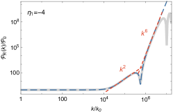
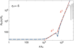
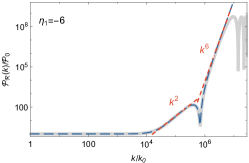
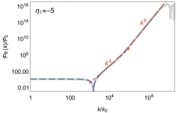
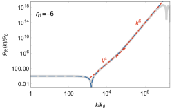
Figure 11: The power spectrums for $N_{2}\ll N_{3}$ in the $\eta_{1}=-4,-5$ and $-6$ cases. The gray-solid and blue-dashed lines represent the numerical and approximate results, respectively. The first line is corresponding to the $c_{s_{1}}^{2}e^{-(3+\eta_{1})N_{3}}\ll 1$ case and the second line to the $c_{s_{1}}^{2}e^{-(3+\eta_{1})N_{3}}\gg 1$ case.

Furthermore, when $\eta_{1}=-1$ and $-3$ there are singularities in Eq. (38) and thus these cases need to be studied separately. To avoid the problem, we first set the value of $\eta_{1}$, and then expand Eq. (34) in the infrared limit to obtain

$$\widetilde{\mathcal{R}}^{(2)}_{k}(\tau)=\left\{\begin{array}[]{ll}\dfrac{iHe^{-ik\tau_{1}}}{2\sqrt{\epsilon_{0}k^{3}}}-\dfrac{H\tau_{1}e^{-ik\tau_{1}}}{2\sqrt{\epsilon_{0}k}}-\dfrac{iHc_{s_{1}}^{2}e^{-ik\tau_{1}}k^{1/2}}{8\sqrt{\epsilon_{0}}}\left[2\tau_{1}^{2}+\tau_{2}^{2}-(-\tau)^{2}\right]+\dots&\eta_{1}=-1\vspace{0.4cm}\\ \dfrac{iHe^{-ik\tau_{1}}}{2\sqrt{\epsilon_{0}k^{3}}}-\dfrac{H\tau_{1}e^{-ik\tau_{1}}}{2\sqrt{\epsilon_{0}k}}-\dfrac{iHc_{s_{1}}^{2}e^{-ik\tau_{1}}k^{1/2}}{8\sqrt{\epsilon_{0}}}\left[2\tau_{1}^{2}-3\tau_{2}^{2}-6\tau_{2}^{2}\log\left(\dfrac{\tau}{\tau_{2}}\right)\right]+\dots&\eta_{1}=-3\ .\\ \end{array}\right.$$

In the case of $\eta_{1}=-1$, the solution consists of constant and decaying terms, and thus it is dominated by the constant terms. When $\eta_{1}=-3$, except for the constant terms, the solution of the curvature perturbations contains a logarithmic-growing term. This character is different from that in the $\eta_{1}<-3$ case, where the growth of the solution is power law. Since the coefficient of the logarithmic-growing term depends on $c_{s_{1}}^{2}$, which is much less than one in our analysis, the contribution of the growth term in the solution is negligible. Thus, from Eq. (52), we obtain that the power spectrum has the same expression

$$\dfrac{\mathcal{P}_{\widetilde{\mathcal{R}}^{(2)}_{k}}}{\mathcal{P}_{0}}\simeq 1+\tau_{1}^{2}k^{2}+\dfrac{1}{4}c_{s_{1}}^{4}\tau_{1}^{4}k^{4}$$ (52)

for $\eta_{1}=-1$ and $-3$. The steepest growth is $k^{2}$ apparently. The corresponding numerical and approximate results of the power spectrum are shown in Fig. 12.

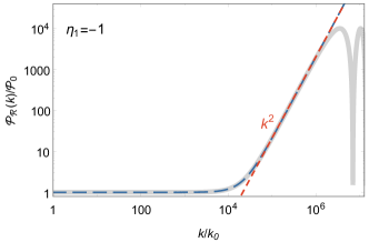
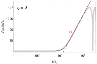
Figure 12: The power spectrums in the $\eta_{1}=-1$ and $\eta_{1}=-3$ cases. The gray-solid and blue-dashed lines represent the numerical and approximate results, respectively.

III.3 Changes of slow-roll parameter $\eta$ previous to the sound speed

This scenario is shown in Fig. 13. The slow-roll parameter $\eta$ changes from $\sim 0$ to a negative constant $\eta_{1}$ at $\tau_{1}$, and the sound speed decreases from $1$ to a small constant $c_{s_{1}}$ at $\tau_{2}$ ($|\tau_{2}|<|\tau_{1}|$).

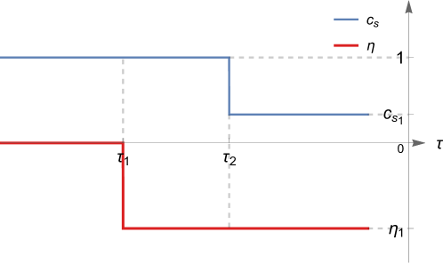
Figure 13: The sound speed $c_{s}$ (blue line) varies at $\tau_{2}$, and the slow-roll parameter $\eta$ (red line) changes at $\tau_{1}$ $(|\tau_{2}|<|\tau_{1}|$).

Since the method for analytical solution in this case is similar to that of the preceding subsection, we do not give the details here. The general expression of the curvature perturbations in the infrared region ($-c_{s_{1}}k\tau\rightarrow 0$, $-c_{s_{1}}k\tau_{2}\rightarrow 0$ and $-k\tau_{1}\rightarrow 0$) is so complex, and we do not show it here. We only consider the integer $\eta_{1}$ cases. Different from the results obtained in the preceding subsection, we find that the analytical results do not coincide with the numerical ones when $\eta_{1}=-1$ and $-2$. Therefore, we only give the infrared expressions ($-k\tau_{1}\rightarrow 0,-c_{s_{1}}k\tau_{2}\rightarrow 0$ and $-c_{s_{1}}k\tau\rightarrow 0$) of the curvature perturbations in the $\eta_{1}\leq-3$ case:

$$\hat{\mathcal{R}}^{(2)}_{k}(\tau)=\left\{\begin{array}[]{ll}\dfrac{iH}{2\sqrt{\epsilon_{0}k^{3}}}\\ +\left(\dfrac{iH\left(3\tau_{1}^{2}-\left(1-c_{s_{1}}^{2}\right)\tau_{2}^{2}\right)}{8\sqrt{\epsilon_{0}}}+\dfrac{3iH\tau_{1}^{2}}{4\sqrt{\epsilon_{0}}}\left(c_{s_{1}}^{2}\log\left[\dfrac{\tau}{\tau_{2}}\right]-\log\left[\dfrac{\tau_{1}}{\tau_{2}}\right]\right)\right)k^{1/2}\\ +\left(\dfrac{H\tau_{1}^{3}}{6\sqrt{\epsilon_{0}}}-\dfrac{H\tau_{1}^{3}}{2\sqrt{\epsilon_{0}}}\log\left[\dfrac{\tau_{1}}{\tau_{2}}\right]+\dfrac{c_{s_{1}}^{2}H\tau_{1}^{3}}{2\sqrt{\epsilon_{0}}}\log\left[\dfrac{\tau}{\tau_{2}}\right]\right)k^{3/2}+\dots&\eta_{1}=-3\vspace{0.4cm}\\ \dfrac{iH}{2\sqrt{\epsilon_{0}k^{3}}}\\ -\left(\dfrac{iH\left(\left(1-c_{s_{1}}^{2}\right)\left(8\tau_{1}^{3}+\tau_{2}^{3}\right)-12\tau_{1}^{2}\tau_{2}\right)}{12\sqrt{\epsilon_{0}}\tau_{2}}-\dfrac{2ic_{s_{1}}^{2}H\tau_{1}^{3}}{3\sqrt{\epsilon_{0}}}(-\tau)^{-1}\right)k^{1/2}.\\ -\left(\dfrac{H\tau_{1}^{3}\left(3\left(1-c_{s_{1}}^{2}\right)\tau_{1}-4\tau_{2}\right)}{6\sqrt{\epsilon_{0}}\tau_{2}}-\dfrac{c_{s_{1}}^{2}H\tau_{1}^{4}}{2\sqrt{\epsilon_{0}}}\left(-\tau\right)^{-1}\right)k^{3/2}+\dots&\eta_{1}=-4\vspace{0.4cm}\\ \dfrac{iH}{2\sqrt{\epsilon_{0}k^{3}}}\\ -\left(\dfrac{iH\left(\left(1-c_{s_{1}}^{2}\right)\left(5\tau_{1}^{4}+\tau_{2}^{4}\right)-10\tau_{1}^{2}\tau_{2}^{2}\right)}{16\sqrt{\epsilon_{0}}\tau_{2}^{2}}+\dfrac{5ic_{s_{1}}^{2}H\tau_{1}^{4}}{16\sqrt{\epsilon_{0}}}(-\tau)^{-2}\right)k^{1/2}\\ -\left(\dfrac{H\tau_{1}^{3}\left(3\left(1-c_{s_{1}}^{2}\right)\tau_{1}^{2}-5\tau_{2}^{2}\right)}{12\sqrt{\epsilon_{0}}\tau_{2}^{2}}+\dfrac{c_{s_{1}}^{2}H\tau_{1}^{5}}{4\sqrt{\epsilon_{0}}}\left(-\tau\right)^{-2}\right)k^{3/2}+\dots&\eta_{1}=-5\vspace{0.4cm}\\ \dfrac{iH}{2\sqrt{\epsilon_{0}k^{3}}}\\ -\left(\dfrac{iH\left(\left(1-c_{s_{1}}^{2}\right)\left(4\tau_{1}^{5}+\tau_{2}^{5}\right)-10\tau_{1}^{2}\tau_{2}^{3}\right)}{20\sqrt{\epsilon_{0}}\tau_{2}^{3}}-\dfrac{5ic_{s_{1}}^{2}H\tau_{1}^{5}}{5\sqrt{\epsilon_{0}}}(-\tau)^{-3}\right)k^{1/2}\\ -\left(\dfrac{H\tau_{1}^{3}\left(\left(1-c_{s_{1}}^{2}\right)\tau_{1}^{3}-2\tau_{2}^{3}\right)}{6\sqrt{\epsilon_{0}}\tau_{2}^{3}}-\dfrac{c_{s_{1}}^{2}H\tau_{1}^{6}}{6\sqrt{\epsilon_{0}}}\left(-\tau\right)^{-3}\right)k^{3/2}+\dots&\eta_{1}=-6\ \;.\end{array}\right.$$ (64)

From the above expression, one can obtain the power spectrum:

$$\frac{\mathcal{P}_{\hat{\mathcal{R}}^{(2)}_{k}}}{\mathcal{P}_{0}}\simeq\left\{\begin{array}[]{ll}1+\frac{1}{2}\left(3-e^{-2N_{2}}-6N_{2}-6c_{s_{1}}^{2}N_{3}\right)\tau_{1}^{2}k^{2}\\ ~{}+\frac{1}{16}\left(3-e^{-2N_{2}}-6N_{2}-6c_{s_{1}}^{2}N_{3}\right)^{2}\tau_{1}^{4}k^{4}\\ ~{}+\frac{1}{9}\left(1-3N_{2}-3c_{s_{1}}^{2}N_{3}\right)^{2}\tau_{1}^{6}k^{6}&\eta_{1}=-3\vspace{0.4cm}\\ 1+\frac{1}{3}\left(12-e^{-2N_{2}}-8e^{N_{2}}+8c_{s_{1}}^{2}e^{N_{2}}-8c_{s_{1}}^{2}e^{N_{2}+N_{3}}\right)\tau_{1}^{2}k^{2}\\ ~{}+\frac{1}{36}\left(12-e^{-2N_{2}}-8e^{N_{2}}+8c_{s_{1}}^{2}e^{N_{2}}-8c_{s_{1}}^{2}e^{N_{2}+N_{3}}\right)^{2}\tau_{1}^{4}k^{4}\\ ~{}+\frac{1}{9}\left(4-3e^{N_{2}}+3c_{s_{1}}^{2}e^{N_{2}}-3c_{s_{1}}^{2}e^{N_{2}+N_{3}}\right)^{2}\tau_{1}^{6}k^{6}&\eta_{1}=-4\vspace{0.4cm}\\ 1+\frac{1}{4}\left(10-e^{-2N_{2}}-5e^{2N_{2}}+5c_{s_{1}}^{2}e^{2N_{2}}-5c_{s_{1}}^{2}e^{2N_{2}+2N_{3}}\right)\tau_{1}^{2}k^{2}\\ ~{}+\frac{1}{64}\left(10-e^{-2N_{2}}-5e^{2N_{2}}+5c_{s_{1}}^{2}e^{2N_{2}}-5c_{s_{1}}^{2}e^{2N_{2}+2N_{3}}\right)^{2}\tau_{1}^{4}k^{4}\\ ~{}+\frac{1}{36}\left(5-3e^{2N_{2}}+3c_{s_{1}}^{2}e^{2N_{2}}-3c_{s_{1}}^{2}e^{2N_{2}+2N_{3}}\right)^{2}\tau_{1}^{6}k^{6}&\eta_{1}=-5\vspace{0.4cm}\\ 1+\dfrac{1}{5}\left(10-e^{-2N_{2}}-4e^{3N_{2}}+4c_{s_{1}}^{2}e^{3N_{2}}-4c_{s_{1}}^{2}e^{3N_{2}+3N_{3}}\right)\tau_{1}^{2}k^{2}\\ ~{}+\frac{1}{100}\left(10-e^{-2N_{2}}-4e^{3N_{2}}+4c_{s_{1}}^{2}e^{3N_{2}}-4c_{s_{1}}^{2}e^{3N_{2}+3N_{3}}\right)^{2}\tau_{1}^{4}k^{4}\\ ~{}+\frac{1}{9}\left(2-e^{3N_{2}}+c_{s_{1}}^{2}e^{3N_{2}}-c_{s_{1}}^{2}e^{3N_{2}+3N_{3}}\right)^{2}\tau_{1}^{6}k^{6}&\eta_{1}=-6\ \;.\end{array}\right.$$ (77)

Here $N_{2}$ and $N_{3}$ are the number of $e$-folds during the second and third phase, respectively. The maximum wave number in the infrared limit is $k|\tau_{1}|$. So, in Eq. (77), the wave number must satisfy $k\ll\bar{k}_{c}\equiv-1/\tau_{1}$. When the $k^{6}$ dominant term becomes comparable to the $k^{4}$ one, the wave number should be equal to about

$$k_{3}\simeq\left\{\begin{array}[]{ll}-\dfrac{3}{2\tau_{1}}=\dfrac{3}{2}\bar{k}_{c}{}{}{}{}&\eta_{1}=-3\vspace{0.2cm}\\ -\dfrac{4}{3\tau_{1}}=\dfrac{4}{3}\bar{k}_{c}&\eta_{1}=-4\vspace{0.2cm}\\ -\dfrac{5}{4\tau_{1}}=\dfrac{5}{4}\bar{k}_{c}&\eta_{1}=-5\vspace{0.2cm}\\ -\dfrac{6}{5\tau_{1}}=\dfrac{6}{5}\bar{k}_{c}&\eta_{1}=-6\ .\end{array}\right.$$ (82)

It is obvious that all wave number $k_{3}$ are larger than $\bar{k}_{c}$ and thus are beyond the infrared region, which means that the steepest growth of the power spectrum is $k^{4}$. Furthermore, we find that the power spectrum will dip before the $k^{4}$ growth. The corresponding numerical and approximate results are shown in Fig. 14.

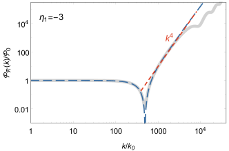
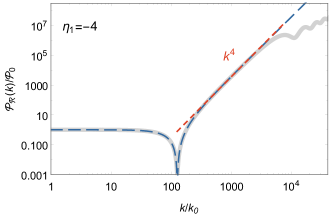
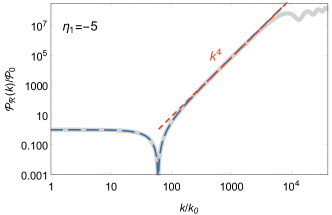
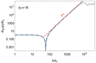
Figure 14: The power spectrums for different constant values of $\eta_{1}$. The gray-solid and blue-dashed lines represent the numerical and approximate results, respectively.

IV conclusions

The generation of a significant amount of primordial black holes requires a sufficiently large power spectrum of the curvature perturbations of the order of about $\mathcal{O}(10^{-2})$ at the scales smaller than the CMB one. There are two natural ways to amplify the curvature perturbations. One is to reduce the rolling speed of the inflaton and the other to suppress the sound speed $c_{s}$ of the curvature perturbations. In the ultraslow-roll inflation scenario, it has been found that the power spectrum of the curvature perturbations has the $k^{4}$ growth. In this paper, we use the improved junction conditions to find that the power spectrum of the curvature perturbation has a $k^{2}$ growth when the speed of sound decreases suddenly. Furthermore, by investigating the evolution of the power spectrum in the inflation model, which can realize decrease of both the sound speed and the rolling speed of the inflaton, we find that the power spectrum at the large scales is nearly scale invariant to satisfy the constraint from the CMB observations, and at the same time it will be enhanced at the small scales to achieve an abundant formation of primordial black holes. In the cases that the change of the slow-roll parameter $\eta$ precedes that of the sound speed $c_{s}$, the power spectrum of the curvature perturbations only has a $k^{4}$ growth. While if $\eta$ and $c_{s}$ changes simultaneously or the change of $c_{s}$ precedes that of $\eta$, the power spectrum can possess a $k^{6}$ growth under certain conditions, which is the steepest growth of the power spectrum reported analytically so far. In the multifield inflation, numerical results show that the growth larger than $k^{6}$ is possible due to the violent tachyonic instability Braglia2020 ; Palma2020 ; Fumagalli2023 ; Braglia2021 ; Braglia2023 .