Capacity Bounds for Hyperbolic Neural Network Representations of Latent Tree Structures

Abstract

We study the representation capacity of deep hyperbolic neural networks (HNNs) with a ReLU activation function. We establish the first proof that HNNs can $\varepsilon$-isometrically embed any finite weighted tree into a hyperbolic space of dimension $d$ at least equal to $2$ with prescribed sectional curvature $\kappa<0$, for any $\varepsilon>1$ (where $\varepsilon=1$ being optimal). We establish rigorous upper bounds for the network complexity on an HNN implementing the embedding. We find that the network complexity of HNN implementing the graph representation is independent of the representation fidelity/distortion. We contrast this result against our lower bounds on distortion which any ReLU multi-layer perceptron (MLP) must exert when embedding a tree with $L>2^{d}$ leaves into a $d$-dimensional Euclidean space, which we show at least $\Omega(L^{1/d})$; independently of the depth, width, and (possibly discontinuous) activation function defining the MLP.

Keywords: Generalization Bounds, Graph Neural Networks, Digital Hardware, Discrete Geometry, Metric Embeddings, Discrete Optimal Transport, Concentration of Measure.

MSC (2022): 68T07, 30L05, 68R12, 05C05.

1 Introduction

Trees are one of the most important hierarchical data structures in computer science, whose structure can be exploited to yield highly efficient algorithms. For example, leveraging the tree’s hierarchical structure to maximize parameter search efficiency, as in branch-and-bound algorithms Land and Doig (2010) or depth-first searches Korf (1985). Consequentially, algorithms designed for trees and algorithms which map more general structures into trees, e.g. Fuchs et al. (1980), have become a cornerstone of computer science and its related areas. Nevertheless, it is known that the flat Euclidean geometry of $\mathbb{R}^{d}$ is fundamentally different from the expansive geometry of trees which makes them difficult to embed into low dimensional Euclidean space with low distortion Bourgain (1986); Matoušek (1999); Gupta (2000). This high distortion can be problematic for downstream tasks relying on Euclidean representations of such trees. This fundamental impasse in representing large trees with Euclidean space has sparked the search for non-Euclidean representation spaces whose geometry is tree-like, thus allowing for low-dimensional representation of arbitrary trees. One such family of representation spaces are the hyperbolic spaces $\mathbb{H}^{d}$, $d\geq 2$, which have recently gained traction in machine learning.

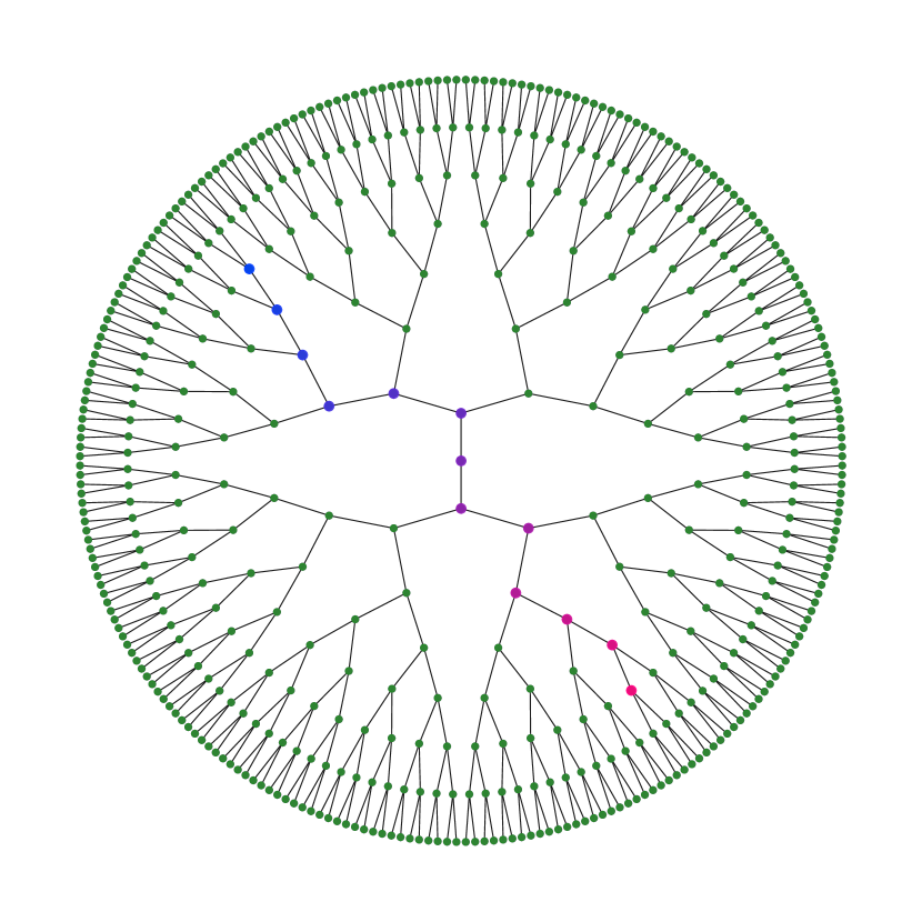
(a) Binary Tree (green) with a coloured minimal length curve in blue-red.

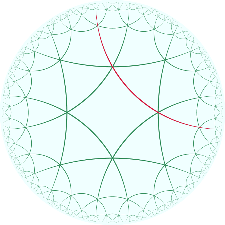
(b) The two-dimensional hyperbolic space $\mathbb{H}^{2}$ with minimal length curves in red.

Figure 1.1: Minimal length curves in the hyperbolic space(right) expand outwards exponentially quickly just as the number of nodes double exponentially rapidly in a tree (right) as one travels away from the origin/root.

Leveraging hyperbolic data representations with a (latent) tree-like structure has proven significantly more effective than their traditional Euclidean counterparts. Machine learning examples include learning linguistic hierarchies Nikiel (1989), natural language processing Ganea et al. (2018a); Zhu et al. (2020b), recommender systems Vinh Tran et al. (2020); Skopek et al. (2020), low-dimensional representations of large tree-like graphs Ganea et al. (2018b); Law and Stam (2020); Kochurov et al. (2020); Zhu et al. (2020a); Bachmann et al. (2020); Sonthalia and Gilbert (2020), knowledge graph representations Chami et al. (2020), network science Papadopoulos et al. (2014); Keller-Ressel and Nargang (2020), communication Kleinberg (2007), deep reinforcement learning Cetin et al. (2023), and numerous other recent applications.

These results have motivated deep learning on hyperbolic spaces, of which the hyperbolic neural networks (HNNs) Ganea et al. (2018a), and their several variants Gulcehre et al. (2018); Chami et al. (2019); Shimizu et al. (2021); Zhang et al. (2021) have assumed the role of the flagship deep learning model. This has led HNNs to become integral in several deep learning-power hyperbolic learning algorithms and have also fuelled applications ranging from natural language processing Ganea et al. (2018a); Dhingra et al. (2018); Tay et al. (2018); Liu et al. (2019); Zhu et al. (2020b), to latent graph inference for downstream graph neural network (GNN) optimization Kazi et al. (2022); de Ocáriz Borde et al. (2022). Furthermore, the simple structure of HNNs makes them amenable to mathematical analysis, similarly to multi-layer perceptrons (MLPs) in classical deep learning. This has led to the establishment of their approximation capabilities in Kratsios and Bilokopytov (2020); Kratsios and Papon (2022).

The central motivation behind HNNs is that they are believed to be better suited to representing data with latent tree-like, or hierarchical, structure than their classical $\mathbb{R}^{n}$-valued counterparts; e.g. MLPs, CNNs, GNNs, or Transformers, since the geometry of hyperbolic space $\mathbb{H}^{d}$, $d\geq 2$, is most similar to the geometry of trees than classical Euclidean space, see Figure 1. These intuitions are often fueled by classical embedding results in computer science Sarkar (2011), metric embedding theory Bonk and Schramm (2000), and the undeniable success of countless algorithms leveraging hyperbolic geometry Papadopoulos et al. (2012, 2014); Nickel and Kiela (2017); Balazevic et al. (2019); Sonthalia and Gilbert (2020); Keller-Ressel and Nargang (2020) for representation learning. Nevertheless, the representation potential of HNNs, in representing data with latent hierarchies, currently only rests on strong experimental evidence, expert intuition rooted in deep results from hyperbolic geometry Gromov (1981, 1987); Bonk and Schramm (2000).

In this paper, we examine the problem of Euclidean-vs-hyperbolic representation learning when a latent hierarchy structures the data. We justify this common belief by first showing that HNNs can $\varepsilon$-isometrically embed any pointcloud with a latent weighted tree structure for any $\varepsilon>0$. In contrast, such an embedding cannot exist in any Euclidean space. We show that the HNNs implementing these $\varepsilon$-embeddings are relatively small by deriving upper bounds on their depth, width, and number of trainable parameters sufficient for achieving any desired representation capacity. We find that HNNs only require $\widetilde{\mathcal{O}}(N^{2})$ trainable parameters to embed any $N$-point pointcloud in $n$-dimensional Euclidean space, with a latent tree structure, into the $2$-dimensional hyperbolic plane.

We then return to the problem of Euclidean-vs-hyperbolic representation under a latent hierarchical structure, by proving that any MLP cannot faithfully embed them into a low-dimensional Euclidean space, thus proving that HNNs are superior to MLPs for representing tree-like structures. We do so by showing that any MLP, regardless of its depth, width, or number of trainable parameters, cannot embed a pointcloud with latent tree structure, with $L>2^{d}$ leaves, into the $d$-dimensional Euclidean space with distortion less than $\Omega(L^{1/d})$. We consider the distortion of an embedding as in the classical computer science literature, e.g. Linial et al. (1995); Bartal (1996); Gupta (2000); a formal definition will be given in the main text.

Outline

The rest of this paper is organized as follows. Section 2 introduces the necessary terminologies for hyperbolic neural networks, such as the geometry of hyperbolic spaces and the formal structure of HNNs. Section 3 formalizes latent tree structures and then numerically formalizes the representation learning problem.

Our main graph representation learning results are given in Section 4.2. In Section 4.1, we first derive lower bounds for the best possible distortion achievable by an MLP representation of a latent tree. We show that MLPs cannot embed any large tree in a small Euclidean space, irrespective of how many wide hidden layers the network uses and irrespective of which, possibly discontinuous, non-linearity is used to define the MLP. In Section 4.2, we show that HNNs can represent any pointcloud with a latent tree structure to arbitrary precision. Furthermore, the depth, width, and number of trainable parameters defining the HNN are independent of the representation fidelity/distortion. Our theory is validated experimentally in Section 4.3. The analysis and proofs of our main results are contained in Section 5. We draw our conclusions in Section 6.

2 The Hyperbolic Neural Network Model

Throughout this paper, we consider hyperbolic neural networks (HNNs) with the $\operatorname{ReLU}(t)\stackrel{{\scriptstyle\mbox{\tiny def.}}}{{=}}\max\{0,t\}$ (Rectified Linear Unit) activation function/non-linearity, mapping into hyperbolic representation spaces $\mathbb{H}^{d}_{\kappa}$. This section rigorously introduced the HNN architecture. This requires a brief overview of hyperbolic spaces, which we do now.

2.1 The Geometry of the Hyperbolic Spaces $\mathbb{H}^{d}_{\kappa}$

Fix a positive integer $d$ and a (sectional) curvature parameter $\kappa<0$. The (hyperboloid model for the real) hyperbolic $d$-space of constant sectional curvature $\kappa$, denoted by $\mathbb{H}^{d}_{\kappa}$, consists of all points $x\in\mathbb{R}^{1+d}$ satisfying

$$1+\sum_{i=1}^{d}\,x_{i}^{2}=x_{d+1}^{2}\mbox{ and }x_{d+1}>0$$

where the distance between any pair of point $x,y\in\mathbb{H}^{d}$ is given by

$$d_{\kappa}(x,y)\stackrel{{\scriptstyle\mbox{\tiny def.}}}{{=}}\frac{1}{\sqrt{|\kappa|}}\,\operatorname{cosh}\Big{(}x_{d+1}y_{d+1}-\sum_{i=1}^{d}\,x_{i}y_{i}\Big{)}.$$

It can be shown that $\mathbb{H}^{d}_{\kappa}$ is a simply connected smooth manifold (Bridson and Haefliger, 1999, pages 92-93) and that the metric $d_{\kappa}$ on any such $\mathbb{H}^{d}_{\kappa}$ measures the length of the shortest curve joining any two points on $\mathbb{H}^{d}_{\kappa}$ where length is quantified in the infinitesimal Riemannian sense (Bridson and Haefliger, 1999, Propositions 6.17 (1) and 6.18). This means that, by the Cartan-Hadamard Theorem (Jost, 2017, Corollary 6.9.1), for every $x\in\mathbb{H}^{d}_{\kappa}$ there is a map $\operatorname{exp}_{{x}}:T_{x}(\mathbb{H}^{d}_{\kappa})\cong\mathbb{R}^{d}\rightarrow\mathbb{H}^{d}_{\kappa}$ which puts $\mathbb{R}^{d}$ into bijection with $\mathbb{H}^{d}$ in a smooth manner with smooth inverse.

Remark 1

Often the metric $d_{\kappa}$ is not relevant for a given statement, and only the manifold structure of $\mathbb{H}^{d}_{\kappa}$ matters, or the choice of $\kappa$ is clear from the context. In these instances, we write $\mathbb{H}^{d}$ in place of $\mathbb{H}^{d}_{\kappa}$ to keep our notation light.

For any point $x\in\mathbb{R}^{d}$, we identify with the $d$-dimensional affine subspace $T_{x}(\mathbb{H}^{d})$ of $\mathbb{R}^{d+1}$ lying tangent to $\mathbb{H}^{d}$ at $x$. For any $x\in\mathbb{H}^{d}$, the tangent space $T_{x}(\mathbb{H}^{d})$ is the $d$-dimensional affine subspace of $\mathbb{R}^{d+1}$ consisting of all $y\in\mathbb{R}^{d+1}$ satisfying

$$y_{d+1}x_{d+1}=\sum_{i=1}^{d}\,y_{i}x_{i}.$$

The tangent space at $\boldsymbol{1}_{n}$ plays an especially important role since its elements can be conveniently identified with $\mathbb{R}^{d}$. This is because $x\in T_{{\boldsymbol{1}_{n}}}(\mathbb{H}^{n})$ only if it is of the form $x=(x_{1},\dots,x_{n},1)$, for some $x_{1},\dots,x_{n}\in\mathbb{R}$. Thus,

$$(x_{1},\dots,x_{n},1)\overset{\pi_{n}}{\rightarrow}(x_{1},\dots,x_{n})\mbox{ and }(x_{1},\dots,x_{n})\overset{\iota_{n}}{\rightarrow}(x_{1},\dots,x_{n},1)$$ (1)

identify $T_{{\boldsymbol{1}_{n}}}(\mathbb{H}^{n})$ with $\mathbb{R}^{n}$.

The map $\operatorname{exp}_{{x}}$ can be explicitly described as the map which sends any “initial velocity vector” $v\in\mathbb{R}^{d}$ lying tangent to $x\in\mathbb{H}^{d}$ to the unique point in $\mathbb{H}^{d}$ which one would arrive at by travelling optimally thereon. Here, optimally means along the unique minimal length curve in $\mathbb{H}^{d}_{-1}$, illustrated in Figure 1(b) . The (affine) tangent spaces $T_{x}(\mathbb{H}^{d})$ and $T_{y}(\mathbb{H}^{d})$ about any two points $x$ and $y$ in $\mathbb{H}^{d}$ are identified by “sliding” $T_{x}(\mathbb{H}^{d})$ towards $T_{y}(\mathbb{H}^{d})$ in parallel across the minimal unique length curve joining $x$ to $y$ in $\mathbb{H}^{d}$. This “sliding” operation, called parallel transport, is formalized by the linear isomorphism $P_{x\mapsto b}:T_{x}(\mathbb{H}^{n})\rightarrow T_{b}(\mathbb{H}^{n})$ given for any $u\in T_{x}(\mathbb{H}^{n})$ by

$$P_{x\mapsto b}:\,u\mapsto u-\frac{\langle\operatorname{log}_{{x}}({b}),u\rangle_{x}}{d_{-1}^{2}(x,b)}\,\big{(}\log_{x}(b)+\log_{b}(x)\big{)},$$ (2)

where the map $\operatorname{log}_{{x}}:\mathbb{R}^{d}\rightarrow\mathbb{H}^{d}$ is defined for any $y\in\mathbb{H}^{d}$ by

$$\operatorname{log}_{{x}}:y\mapsto\frac{d_{-1}(x,y)(y-\langle x|y\rangle_{M}x)}{\|y-\langle x|y\rangle_{M}x\|_{2}},$$

and where $\|\cdot\|_{2}$ is the usual Euclidean norm on $\mathbb{R}^{d+1}$. Typically parallel transport must be approximated numerically, e.g. Guigui and Pennec (2022), but this is not so for $\mathbb{H}^{d}_{-1}$.

The hyperbolic space is particularly convenient, amongst negatively curved Riemannian manifolds, since the map $\operatorname{exp}_{{x}}$ is available in closed-form. For any $x\in\mathbb{H}^{d}_{\kappa}$ and $v\in\mathbb{R}^{d}$, $\operatorname{exp}_{{x}}(v)$ is given by: $\operatorname{exp}_{{x}}(v)=x$ if $v=0$, otherwise

$$\operatorname{exp}_{{x}}:v\mapsto\operatorname{cosh}\big{(}\sqrt{\langle v|v\rangle_{M}}\big{)}+\operatorname{sinh}\big{(}\sqrt{\langle v|v\rangle_{M}}\big{)}\,\frac{v}{\langle v|v\rangle_{M}}$$

where $\langle u|v\rangle_{M}\stackrel{{\scriptstyle\mbox{\tiny def.}}}{{=}}-u_{d+1}v_{d+1}+\sum_{i=1}^{d}\,u_{i}v_{i}$ for any $u,v\in\mathbb{R}^{d}$; see (Bridson and Haefliger, 1999, page 94). Furthermore, the inverse of $\operatorname{exp}_{{x}}$ is $\operatorname{log}_{{x}}$.

We note that these operations are implemented in most standard geometric machine learning software, e.g. Boumal et al. (2014); Townsend et al. (2016); Miolane et al. (2020). Also, $\mathbb{H}_{\kappa}^{d}$ and $\mathbb{H}_{-1}^{d}$ are diffeomorphic by the Cartan-Hadamard Theorem (Jost, 2017, Corollary 6.9.1). Therefore, for all $\kappa<0$, it suffices to consider the “standard” exponential map $\operatorname{exp}_{{x}}$ in the particular case where $\kappa=-1$ to map encode in $\mathbb{R}^{d}$ into $\mathbb{H}^{d}$ and visa-versa via $\operatorname{log}_{{x}}$.

2.2 The Hyperbolic Neural Network Model

We now overview the hyperbolic neural network model studied in this paper. The considered HNN model contains the hyperbolic neural networks of Ganea et al. (2018a), from the deep approximation theory Kratsios and Papon (2022), and the latent graph inference de Ocáriz Borde et al. (2022) literatures as sub-models. The workflow of the hyperbolic neural network’s layer, by which it processes data on the hyperbolic space $\mathbb{H}^{n}$, is summarized in Figure 2.2.

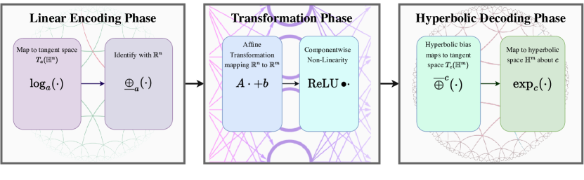
Figure 2.2: Workflow of an HNN layer: First inputs in a hyperbolic space $\mathbb{H}^{n}$ are mapped to a vector in $\mathbb{R}^{n}$ in the “encoding phase”. Next, they are transformed to “deep features” in $\mathbb{R}^{m}$ by a standard MLP layer in the “transformation phase”. Finally, the “hyperbolic decoding phase” applies a hyperbolic bias, at which point the “deep features with hyperbolic bias” are decoded, thus producing an output in the hyperbolic space $\mathbb{H}^{m}$.

HNNs function similarly to standard MLPs, which generate predictions from any input by sequentially applying affine maps interspersed with non-affine non-linearities, typically via component-wise activation functions. Instead of leveraging affine maps, which are otherwise suited to the vectorial geometry of $\mathbb{R}^{d}$, HNNs are built using analogues of the affine maps for Euclidean spaces, which are suited to the geometry of $\mathbb{H}^{2}$. Thus, the analogues of the linear layers with component-wise $\operatorname{ReLU}(t)\stackrel{{\scriptstyle\mbox{\tiny def.}}}{{=}}\max\{0,t\}$ activation function, mapping $\mathbb{H}^{n}$ to $\mathbb{H}^{m}$ for $n,m\in\mathbb{N}_{+}$, are thus given by

$$x\mapsto\operatorname{exp}_{{{\boldsymbol{1}}_{n}}}({\operatorname{ReLU}\bullet(A\operatorname{log}_{{{\boldsymbol{1}}_{m}}}(x))})$$ (3)

where $\bullet$ denotes component-wise composition and $A$ is an $m\times n$ matrix, and ${\boldsymbol{1}}_{n}\in\mathbb{H}^{n}$. Thus, as discussed in (Ganea et al., 2018a, Theorem 4 and Lemma 6), without the “hyperbolic bias” term, the elementary layers making up HNNs can be viewed as elementary MLP layers conjugated by the maps $\operatorname{exp}_{{{\boldsymbol{1}}_{n}}}$ and $\operatorname{log}_{{{\boldsymbol{1}}_{m}}}$. In this case, $\operatorname{exp}_{{{\boldsymbol{1}}_{n}}}$ and $\operatorname{log}_{{{\boldsymbol{1}}_{m}}}$ serve simply to respectively encode and decode the hyperbolic features into vectorial data, which can be processed by standard software.

The analogues of the addition of a bias term were initially formalized in Ganea et al. (2018a) using the so-called gyro-vector addition and multiplication operators; see Vermeer (2005), which roughly states that a bias $b\in\mathbb{H}^{n}$ can be added to any $x\in\mathbb{H}^{n}$ by “shifting by” $b$ along minimal length curves in $\mathbb{H}^{n}$ using $\operatorname{exp}_{{b}}$. Informally,

$$y\mapsto\operatorname{exp}_{{b}}({P_{{\boldsymbol{1}}_{n}\mapsto b}\circ\operatorname{log}_{{0}}({y})})$$ (4)

where $P_{{\boldsymbol{1}}_{n}\mapsto b}:T_{{\boldsymbol{1}}_{n}}(\mathbb{H}^{n})\rightarrow T_{b}(\mathbb{H}^{n})$ linearly identifies the tangent space at ${\boldsymbol{1}}_{n}\stackrel{{\scriptstyle\mbox{\tiny def.}}}{{=}}$ $(0,\dots,0,1)$ with that at $b$ by travelling along the unique minimal length curve in $\mathbb{H}^{n}_{-1}$, defined by $d_{-1}$, connecting ${\boldsymbol{1}}_{n}$ to $b$. The interpretation of (4) as the addition of a bias term dates back at least to early developments in geometric machine learning in Pennec (2006); Meyer et al. (2011); Fletcher (2013). The basic idea is that in the Euclidean space, the analogues of the $\operatorname{exp}_{{x}}$ and $\operatorname{log}_{{x}}$ are simply addition and subtraction, respectively.

Here, we consider a generalization of the elementary HNN layers of Ganea et al. (2018a), used in (Kratsios and Papon, 2022, Corollaries 23 and 24) to constructing universal deep learning models capable of approximating continuous functions between any two hyperbolic spaces. The key difference here is that they, and we, also allowed for a “Euclidean bias” to be added in together with the hyperbolic bias computed by (4). Similar HNN layers are also used in the contemporary latent graph inference literature de Ocáriz Borde et al. (2022); Kazi et al. (2022). Incorporating this Euclidean bias, with the elementary maps (4), the hyperbolic biases (3), and the formal identifications (1) we obtain our elementary hyperbolic layers $\mathcal{L}_{a,b,c,A}:\mathbb{H}^{n}\rightarrow\mathbb{H}^{m}$ maps given by

$$\mathcal{L}_{a,b,c,A}:x\mapsto\operatorname{exp}_{{c}}\biggl{(}\overline{\oplus}^{c}\Big{(}\operatorname{ReLU}\bullet\big{(}A\,\underline{\oplus}_{a}\circ\operatorname{log}_{{a}}({x})+b\big{)}\Big{)}\biggr{)}$$ (5)

where weight matrix $A$ is an $m\times n$ matrix, a Euclidean bias $b\in\mathbb{R}^{n}$, and the incorporation of hyperbolic biases $a\in\mathbb{H}^{n}$ and $b\in\mathbb{H}^{m}$ are defined by

$$\overline{\oplus}^{c}\stackrel{{\scriptstyle\mbox{\tiny def.}}}{{=}} P_{{\boldsymbol{1}_{m}\mapsto c}}\circ\iota_{m}:\mathbb{R}^{m}\rightarrow T_{c}(\mathbb{H}^{m})$$

$$\underline{\oplus}_{a}\stackrel{{\scriptstyle\mbox{\tiny def.}}}{{=}} \pi_{n}\circ P_{a\mapsto\boldsymbol{1}_{n}}:T_{a}(\mathbb{H}^{n})\rightarrow\mathbb{R}^{n}.$$

The number of trainable parameters defining any hyperbolic layer $\mathcal{L}_{a,b,c,A}$ is

$$\operatorname{Par}(\mathcal{L}_{a,b,c,A})\stackrel{{\scriptstyle\mbox{\tiny def.}}}{{=}}\|A\|_{0}+\|a\|_{0}+\|b\|_{0}+\|c\|_{0}$$ (6)

where $\|\cdot\|_{0}$ counts the number of non-zero entries in a matrix or vector.

We work with data represented as vectors in $\mathbb{R}^{n}$ with a latent tree structure. Similarly to de Ocáriz Borde et al. (2022); Kazi et al. (2022), these can be encoded as hyperbolic features, making them compatible with standard HNN pipelines, using $\operatorname{exp}_{{\boldsymbol{1}_{n}}}$ as a feature map. Any such feature map is regular in that it preserves the approximation capabilities of any downstream deep learning model, see (Kratsios and Bilokopytov, 2020, Corollary 3.16) for details.

Definition 2 (Hyperbolic Neural Networks)

Let $n,d\in\mathbb{N}_{+}$. A function $f:\mathbb{R}^{n}\rightarrow\mathbb{H}^{d}$ is called a hyperbolic neural network (HNN) if it admits the iterative representation: for any $x\in\mathbb{R}^{n}$

$$f(x) =\operatorname{exp}_{{c^{(I+1)}}}\Big{(}\overline{\oplus}^{c^{(I+1)}}\big{(}A^{(I+1)}\,(\underline{\oplus}_{c^{(I)}}\circ\operatorname{log}_{{c^{(I)}}}({x^{(I)}})+b^{(I+1)})\big{)}\Big{)}$$

$$x^{(i)} =\mathcal{L}_{c^{(i-1)},b^{(i)},c^{(i)},A^{(i)}}(x^{(i-1)})\qquad\qquad\qquad\qquad\qquad\qquad\mbox{for }i=1,\dots,I$$

$$x^{(0)} =\operatorname{exp}_{{c^{(0)}}}(\overline{\oplus}^{c^{(0)}}\,x)$$

where $I\in\mathbb{N}_{+}$, $n=d_{0},\dots,d_{I+2}=d\in\mathbb{N}_{+}$, and for $i=1,\dots,I+1$, $A^{(i)}$ is a $d_{i+1}\times d_{i}$ matrix, $b^{(i)}\in\mathbb{R}^{d_{i}}$, $c^{(i)}\in\mathbb{H}^{d_{i+1}}\subset\mathbb{R}^{d_{i+1}+1}$, and $c^{(0)}\in\mathbb{H}^{n}\subset\mathbb{R}^{n+1}$.

In the notation of Definition 2, the integer $I+1$ is called the depth of the HNN $f$ and the width of $f$ is $\max_{i=0,\dots,I+1}\,d_{i}$. Similarly to (6), the total number of trainable parameters defining the HNN $f$, denoted by $\operatorname{Par}(f)$, is tallied by

$$\operatorname{Par}(f)\stackrel{{\scriptstyle\mbox{\tiny def.}}}{{=}}\|c^{(0)}\|_{0}+\sum_{i=1}^{I+1}\,\|A^{(i)}\|_{0}+\|b^{(i)}\|_{0}+\|c^{(i)}\|_{0}.$$

Note that, since the hyperbolic bias $c^{(i)}$ is shared between any two subsequent layers, in the notation of (6) $\alpha=c^{(i-1)}$ and $c=c^{(i)}$ for any $i=1,\dots,I+1$, then we do not double count these parameters.

3 Representing Learning with Latent Tree Structures

We now formally define latent tree structures. These capture the actual hierarchical structures between points in a pointcloud. We then formalize what it means to represent those latent tree structures in an ideally low-dimensional representation space with little distortion. During this formalization process we will recall some key terminologies pertaining to trees.

3.1 Latent Tree Structure

We now formalize the notation of a latent tree structure between members of a pointclouds a vector space $\mathbb{R}^{n}$. We draw from ideas in clustering, where the relationship between pairs of points is not captured by reflected by their configuration in Euclidean space but rather through some unobservable latent distance/structure. Standard examples from the clustering literature include the Mahalanobis distance Xiang et al. (2008), the Minkowski distance or $\ell^{\infty}$ distances Singh et al. (2013), which are implemented in standard software Achtert et al. (2008); De Smedt and Daelemans (2012), and many others; e.g. Ye et al. (2017); Huang et al. (2023); Grande and Schaub (2023).

In the graph neural network literature, the relationship between pairs of points is quantified graphically. In the cases of latent trees, the relationships between points are induced by a weighted tree graph describing a simple relational structure present in the dataset. The presents of an edge between any two points indicated a direct relationship between two nodes, and the weight of any such edge quantifying the strength of the relationship between the two connected, and thus related, nodes. This relational structure can be interpreted as a latent hierarchy upon specifying a root node in the latent tree.

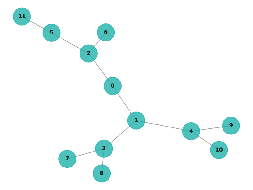
(a)

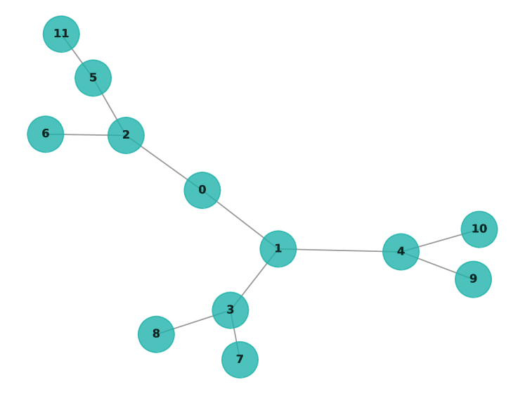
(b)

Figure 3.3: Figures 3(a) and 3(b) illustrate pointclouds in $\mathbb{R}^{2}$ with the same latent tree structure. Both of these trees seem different when comparing their structure using the Euclidean distances; however, instead, considering their latent tree structure reveals that they are identical as graphs. This illustrates how Euclidean geometry often fails to detect the true latent (relational) geometry describing the hierarchical structure between points in a pointcloud.

Let $n$ be a positive integer and $V$ be a non-empty finite subset of $\mathbb{R}^{n}$, called a pointcloud. Illustrated by Figure 3.3, a latent tree structure on $V$ is a triple $(V,\mathcal{E},W)$ of a collection $\mathcal{E}$ of pairs $\{u,v\}$, called edges, of $u,v\in V$ and an edge-weight map $\mathcal{W}:\mathcal{E}\rightarrow(0,\infty)$ satisfying the following property: For every distinct pair $u,v\in V$ there exists a unique sequence $u=u_{0},\dots,u_{i}=v$ of distinct nodes in $V$ such that the edges $\{u_{0},u_{1}\},\dots,\{u_{i-1},u_{i}\}$ belong to $\mathcal{E}$; called a path from $u$ to $v$. Thus, $\mathcal{T}=(V,\mathcal{E},\mathcal{W})$ is a finite weighted tree with positive edge weights.

Any latent tree structure $\mathcal{T}$ on $V$ induces a distance function, or metric, between the points of $V$. This distance function, denoted by $d_{\mathcal{T}}$, measures the length of the shortest path between pairs of points $u,v\in V$ and is defined by

$$d_{\mathcal{T}}(u,v)\stackrel{{\scriptstyle\mbox{\tiny def.}}}{{=}}\inf\,\sum_{j=0}^{i-1}\,\mathcal{W}\big{(}\{u_{j},u_{j+1}\}\big{)}$$

where the infimum is taken over all sequences of paths $\{u_{0},u_{1}\},\dots,\{u_{i-1},u_{i}\}$ from $u=u_{0}$ to $v=u_{i}$.

If the weight function $\mathcal{W}(\{u,v\})=1$ for any edges $\{u,v\}\in\mathcal{E}$, then $\mathcal{T}$ is called a combinatorial tree. In which case, the distance between any two nodes $u,v\in V$ simplifies to the usual shortest path distance on an unweighted graph

$$d_{\mathcal{T}}(u,v)=\inf\big{\{}i\,:\,\exists\,\{v,v_{1}\},\dots\{v_{i-1},u\}\in\mathcal{E}\big{\}}.$$ (7)

The degree of any point, or node/vertex, $v\in V$ is the number of edges emanating from $v$; i.e. the cardinality of $\{\{u,w\}\in\mathcal{E}:\,v\in\{u,w\}\}$. A node $v\in V$ is called a leaf of the tree $\mathcal{T}$ if it has degree $1$. E.g. in Figure 1(a), all peripheral green points are leaves of the binary tree.

3.2 Representations as Embeddings

As in Kratsios et al. (2023), a representation, or encoding, of latent tree structure on $V$ is simply a function $f:V\rightarrow\mathcal{R}$ into a space $\mathcal{R}$ equipped with a distance function $d_{\mathcal{R}}$, the pair $(\mathcal{R},d_{\mathcal{R}})$ of which is called a representation space. As in Giovanni et al. (2022) representation $f$ is considered “good” if it accurately preserves the geometry of the latent tree structure $\mathcal{T}$ on $V$.

Following the classical computer science literature, Linial et al. (1995); Bartal (1996); Rabinovich and Raz (1998); Arora et al. (2009); Magen (2002); STO (2005), this means that $f$ is injective, or $1$-$1$, and its neither shrinks nor stretches the distances between pairs of nodes $u,v\in V$ when compared by $d_{\mathcal{R}}$. For each $u,v\in V$ the following holds

$$\alpha\,d_{\mathcal{T}}(u,v)\leq d_{\mathcal{R}}\big{(}f(u),f(v)\big{)}\leq\beta\,d_{\mathcal{T}}(u,v)$$ (8)

where the constants $0<\alpha\leq\beta<\infty$ are defined by

$$\beta\stackrel{{\scriptstyle\mbox{\tiny def.}}}{{=}}\max_{\begin{subarray}{c}u,v\in V\\ u\neq v\end{subarray}}\,\frac{d_{\mathcal{R}}\big{(}f(u),f(v)\big{)}}{d_{V}(u,v)},\mbox{ and }\alpha\stackrel{{\scriptstyle\mbox{\tiny def.}}}{{=}}\min_{\begin{subarray}{c}u,v\in V\\ u\neq v\end{subarray}}\,\frac{d_{\mathcal{R}}\big{(}f(u),f(v)\big{)}}{d_{V}(u,v)}.$$

These constants quantify the maximal shrinking ($\alpha$) and stretching ($\beta$) which $f$ exerts on the geometry induced by the latent tree structure $\mathcal{T}$ on $V$, and Note that, since $V$ is finite, then $0<\alpha\leq\beta<\infty$ whenever $f$ is injective.

The total distortion with which $f$ perturbs the tree structure $\mathcal{T}$ on $V$ is, denoted by $\operatorname{dist}(f)$, and defined by

$$\operatorname{dist}(f)\stackrel{{\scriptstyle\mbox{\tiny def.}}}{{=}}\begin{cases}\frac{\beta}{\alpha}&\mbox{ : if $f$ is injective}\\ \infty&\mbox{ : otherwise}\end{cases}$$ (9)

We say that a tree $\mathcal{T}$ can be asymptotically isometrically represented in $\mathcal{R}$ if there is a sequence $(f_{n})_{n=1}^{\infty}$ of maps from $V$ to $\mathcal{R}$ whose distortion is asymptotically optimal distortion; i.e. $\lim\limits_{n\rightarrow\infty}\,\operatorname{dist}(f_{n})=1$. We note that a sequence of embeddings $f_{n}$ need not have a limiting function mapping $V$ to $\mathcal{R}$ even if its distortion converges to $1$; in particular, $(f_{n})_{n\in\mathbb{N}}$ need not converge to an isometry.

4 Graph Representation Learning Results

This section contains our main result, which establishes the main motivation behind HNNs, namely the belief that they represent trees to arbitrary precision in a two dimensional hyperbolic space.

4.1 Lower-Bounds on Distortion for MLP Embeddings of Latent Trees

The power of HNNs is best appreciated when juxtaposed against the lower bounds minimal distortion implementable by any MLP embedding any large tree into a low-dimensional Euclidean space. In particular, there cannot exist any MLP model, regardless of its depth, width, or (possibly discontinuous) choice of activation function, which can outperform the embedding of a sufficiently overparameterized HNN using only a two-dimensional representation space.

Theorem 4.1 (Lower-Bounds on the Distortion of Trees Embedded by MLPs)

Let $L,n,d\in\mathbb{N}_{+}$, and fix an activation function $\sigma:\mathbb{R}\rightarrow\mathbb{R}$. For any finite $V\subset\mathbb{R}^{n}$ with a latent combinatorial tree structure $\mathcal{T}=(V,\mathcal{E},\mathcal{W})$ having $L>2^{d}$ leaves and if $f:\mathbb{R}^{n}\rightarrow\mathbb{R}^{d}$ is an MLP with activation function $\sigma$, satisfying

$$\alpha\,d_{\mathcal{T}}(u,v)\leq\|f(u)-f(v)\|\leq\beta\,d_{\mathcal{T}}(u,v)$$

for all $u,v\in V$ and some $0<\alpha\leq\beta$ independent of $u$ and $v$ then, $f$ incurs a distortion $\operatorname{dist}(f)$ of at least

$$\operatorname{dist}(f)\geq\Omega(L^{1/d}).$$

The constant suppressed by $\Omega$, is independent of the depth, width, number of trainable parameters, and the activation function $\sigma$ defining the MLP.

Theorem 4.1 implies that if $V\subseteq\mathbb{R}^{n}$ is large enough and has a latent tree structure with $\Omega(4^{d^{2}})$ leaves then any MLP $f:\mathbb{R}^{n}\rightarrow\mathbb{R}^{d}$ cannot represent $(V,d_{\mathcal{T}})$ with a distortion of less than $\Omega(4^{d})$. Therefore, if $d$, $\#V$, and $L$ are large enough, any MLP must represent the latent tree structure on $V$ arbitrarily poorly. We point out that their MLP’s structure alone is not the cause of this limitation since we have not imposed any structural constraints on its depth, width, number of trainable parameters, or its activation function; instead, the incompatibility between the geometry of a tree and that of a Euclidean space, which no MLP can resolve.

4.2 Upper-Bounds on the Complexity of HNNs Embeddings of Latent Trees

Our main positive result shows that the HNN model 2 can represent any pointcloud with a latent tree structure into the hyperbolic space $\mathbb{H}_{\kappa}^{d}$ with an arbitrarily small distortion by a low-capacity HNN.

Theorem 4.2 (HNNs Can Asymptotically Isometrically Represent Latent Trees)

Fix $n,d,N\in\mathbb{N}_{+}$ with $d\geq 2$ and fix $\lambda>1$. For any $N$-point subset $V$ of $\mathbb{R}^{n}$ and any latent tree structure $\mathcal{T}=(V,\mathcal{E},\mathcal{W})$ on $V$ of degree at least $2$, there exists a curvature parameter $\kappa<0$ and an HNN $f:\mathbb{R}^{n}\rightarrow\mathbb{H}^{d}_{\kappa}$ such that

$$\frac{1}{\lambda}\,d_{\mathcal{T}}(u,v)\leq d_{\kappa}(f(u),f(v))\leq\lambda\,d_{\mathcal{T}}(u,v)$$

holds for each pair of $u,v\in V$. Moreover, the depth, width, and number of trainable parameters defining $f$ are independent of $\lambda$; recorded in Table 1.

Theorem 4.2 considers HNNs with the typical $\operatorname{ReLU}$ activation function. However, using an argument as in (Yarotsky, 2017, Proposition 1) the result can likely be extended to any other continuous piece-wise linear activation function with at least one piece/break, e.g $\operatorname{PReLU}$. Just as in (Yarotsky, 2017, Proposition 1), such modifications should only scale the network depth, width, and the number of its trainable parameters up by a constant factor depending only on the number of pieces of the chosen piece-wise linear activation function.

Since the size of the tree in Theorem 4.2 did not constrain the embedding quality of an HNN, we immediately deduce the following corollary which we juxtapose against Theorem 4.1.

Corollary 4.3 (HNNs Can Asymptotically Embed Large Trees)

Let $L,n,d\in\mathbb{N}_{+}$ with $d\geq 2$. For any finite $V\subset\mathbb{R}^{n}$ with a latent combinatorial tree structure $\mathcal{T}=(V,\mathcal{E},\mathcal{W})$ with $L>2^{d}$ leaves, and any $r>0$, there exists a curvature parameter $\kappa<0$ and an HNN $f:\mathbb{R}^{n}\rightarrow\mathbb{H}^{d}_{\kappa}$ satisfying

$$\operatorname{dist}(f)\leq\frac{1}{L^{r}}.$$

Table 1: Estimates on the Complexity of the HNN implementing the $N$-point memorization of the function $f^{\star}:\mathbb{R}^{n}\rightarrow\mathbb{H}^{d}$ in Lemma 5.1.

Complexity	Upper-Bound
Depth	$\mathcal{O}\left(N\left\{1+\sqrt{N\log{N}}\left[1+\frac{\log(2)}{\log(n)}\left(C_{n}+\frac{\log\left(N^{2}\operatorname{aspect}(V,\|\cdot\|_{2}\right)}{\log(2)}\right)_{+}\right]\right\}\right)$
Width	$n(N-1)+\max\{d,12\}$
N. Train. Par.	$\mathcal{O}\left(N\left(\frac{11}{4}\max\{n,d\}N^{2}-1\right)\left\{d+\sqrt{N\log{N}}\left[1+\frac{\log(2)}{\log(n)}\right.\right.\right.$
	$\left.\left.\times\left(C_{n}+\frac{\log\left(N^{2}\operatorname{aspect}(V,\|\cdot\|_{2}\right)}{\log(2)}\right)_{+}\right]\max\{d,12\}(1+\max\{d,12\})\right\}$
	$+\left.N\left\{1+\sqrt{N\log{N}}\left[1+\frac{\log(2)}{\log(n)}\left(C_{n}+\frac{\log\left(N^{2}\operatorname{aspect}(V,\|\cdot\|_{2}\right)}{\log(2)}\right)_{+}\right]\right\}\right)$

The “dimensional constant” is $0<C_{n}=\frac{2\log(5\sqrt{2\pi})+\frac{3}{2}\log n-\frac{1}{2}\log(n+1)}{2\log(2)}$.

4.3 Experimental Illustrations

To gauge the validity of our theoretical results, we conduct a performance analysis for tree embedding. We compare the performance of HNNs with that of MLPs through a sequence of synthetic graph embedding experiments. Our primary focus lies on binary, ternary, and random trees. For the sake of an equitable comparison, we contrast MLPs and HNNs employing an equal number of parameters. Specifically, all models incorporate 10 blocks of linear layers, accompanied by batch normalization and ReLU activations, featuring 100 nodes in each hidden layer. The training process spans 10 epochs for all models, employing a batch size of 100,000 and a learning rate of $10^{-2}$. The $x$ and $y$ coordinates of the graph nodes in $\mathbb{R}^{2}$ are fed into both the MLP and HNN networks, which are tasked to map them to a new embedding space. An algorithm is used to generate input coordinates, simulating a force-directed layout of the tree. In this simulation, edges are treated as springs, pulling nodes together, while nodes are treated as objects with repelling forces akin to an anti-gravity effect. This simulation iterates until the positions reach a state of equilibrium. The algorithm can be reproduced using the NetworkX library and the spring layout for the graph.

Counting the neighbourhood hops as in 7 defines the distance between nodes, resulting in a scalar value. The networks must discover a suitable representation to estimate this distance. We update the networks based on the MSE loss comparing the actual distance between nodes, $d_{true}$, to the predicted distance based on the network mappings, $d_{pred}$:

$$Loss=MSE(d_{true},d_{pred}).$$ (10)

In the case of the MLP the predicted distance is computed using:

$$d_{pred}=\|MLP(x_{1},y_{1})-MLP(x_{2},y_{2})\|_{2},$$ (11)

where $(x_{1},y_{1})$ and $(x_{2},y_{2})$ are the coordinates in $\mathbb{R}^{2}$ of a synthetically generated latent tree (which may be binary, ternary or random). For the HNN we use the loss function

$$d_{pred}=d_{-1}(HNN(x_{1},y_{1}),HNN(x_{2},y_{2})).$$ (12)

In the case of the HNN, we use the hyperboloid model, with an exponential map at the pole, to map the representations to hyperbolic space. In particular, we do not even require any hyperbolic biases to observe the gap in performance between the MLP and HNN models, which are trained to embed the latent trees by respectively optimizing the loss functions 11 and 12.

We conduct embedding experiments on graphs ranging from 1,000 to 4,000 nodes, and we assess the impact of employing various dimensions for the tree embedding spaces. Specifically, we explore dimensionalities multiples of 2, ranging from 2 to 8. In Figure 4.4, we can observe that HNNs consistently outperform MLPs at embedding trees, achieving a lower MSE error in all configurations.

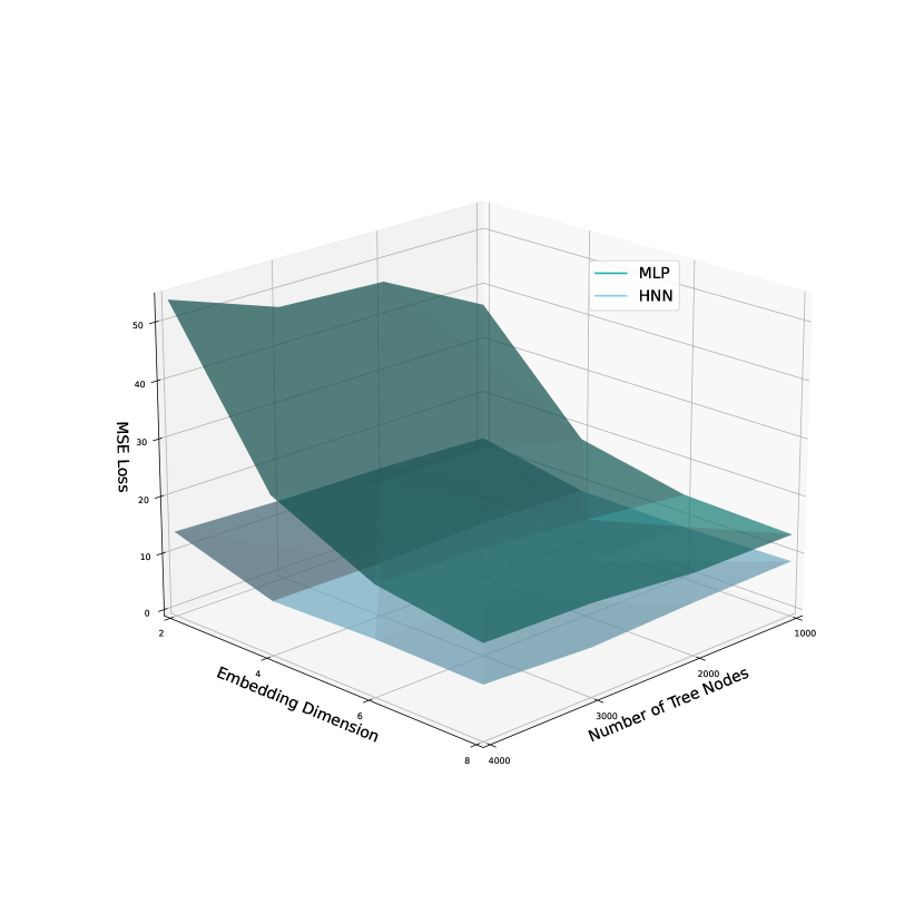
(a) Binary Tree

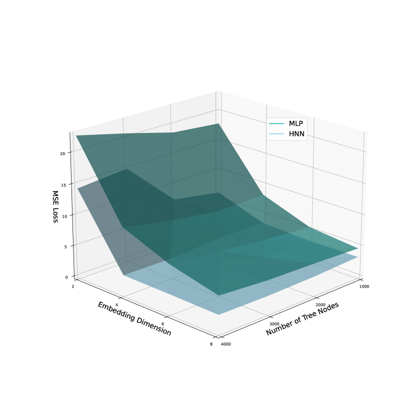
(b) Ternary Tree

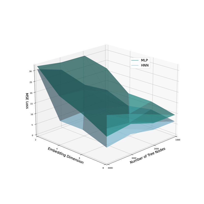
(c) Random Tree

Figure 4.4: Tree embedding error surfaces for different trees using MLPs and HNNs.

We now overview the derivation of our upper bounds on the embedding capabilities HNNs with $\operatorname{ReLU}$ activation function and our lower-bounds on MLPs with any activation function for pointclouds with latent tree structure.

5 Theoretical analysis

We first prove Theorem 4.1 which follows relatively quickly from the classical results of Matoušek (1999) and Gupta (2000) from the metric embedding theory and computer science literature. We then outline the proof of Theorem 4.2, which is much more involved, both technically and geometrically, the details of which are relegated to Section 5. Corollary 4.3 is directly deduced from Theorem 4.2.

5.1 Proof of the Lower-Bound - Theorem 4.1

We begin by discussing the proof of the lower-bound.

Proof [Proof of Theorem 4.1] Any MLP $f:\mathbb{R}^{n}\rightarrow\mathbb{R}^{d}$ with any activation function $\sigma:\mathbb{R}\rightarrow\mathbb{R}$ for which there exists constants $0<\alpha\leq\beta$ satisfying

$$\alpha\,d_{\mathcal{T}}(u,v)\leq\|f(u)-f(v)\|\leq\beta\,d_{\mathcal{T}}(u,v)$$

defines a bi-Lipschitz embedding of the tree-metric space $(V,d_{\mathcal{T}})$ into the $d$-dimensional Euclidean space.

Since $L>2^{d}$ then we may apply (Gupta, 2000, Proposition 5.1), which is a version of a negative result of Bourgain (1986) and of Matoušek (1999) for non-embeddability of large trees in Euclidean space for general trees. The result, namely (Gupta, 2000, Proposition 5.1), implies that any bi-Lipschitz embedding of $(V,d_{\mathcal{T}})$ into $(\mathbb{R}^{d},\|\cdot\|_{2})$ must incur a distortion no less than $\Omega(L^{1/d})$; in particular, this is the case for $f$. Therefore, $\frac{\beta}{\alpha}\geq\Omega(L^{1/d})$.  
The proof of the lower-bound shows that there cannot be any deep learning model which injectively maps $(V,d_{\mathcal{T}})$ into a $d$-dimensional Euclidean space with a distortion of less than $\Omega(L^{1/d})$.

5.2 Proof of Theorem 4.2

We showcase the three critical steps in deriving theorem 4.2. First, we show that HNNs can implement, i.e. memorize, arbitrary functions from any $\mathbb{R}^{n}$ to any $\mathbb{H}^{d}$, for arbitrary integer dimensions $n$ and $d$. Second, we construct a sequence of embeddings with, whose distortion asymptotically tends to $1$, in a sequence of hyperbolic spaces $(\mathbb{H}^{d}_{\kappa},d_{\kappa})$ of arbitrarily large sectional curvature $\kappa$. We then apply our memorization result to deduce that these “asymptotically isometric” embeddings can be implemented by HNNs, quantitatively.

The proofs of both main lemmata are relegated to Section 5.3.

Step 1 - Exhibiting a Memorizing HNN and Estimating its Capacity

We first need the following quantitative memorization guarantee for HNNs.

Lemma 5.1 (Upper-Bound on the Memory Capacity of an HNN)

Fix $N,n,d\in\mathbb{N}_{+}$. For any $N$-point subset $V\subset\mathbb{R}^{n}$ and any function $f^{\star}:\mathbb{R}^{n}\rightarrow\mathbb{H}^{d}$, there exists an HNN $f:\mathbb{R}^{n}\rightarrow\mathbb{H}^{d}$ satisfying

$$f(v)=f^{\star}(v)$$

for each $v\in V$. Moreover, the depth, width, and number of trainable parameters defining $f^{\star}$ are bounded-above in Table 1.

The capacity estimates for the HNNs constructed in Theorem 4.2 and its supporting Lemma 5.1 depend on the configuration of the pointcloud $V$ in $\mathbb{R}^{n}$ with respect to the Euclidean geometry of $\mathbb{R}^{n}$. The configuration is quantified by the ratio of the largest distance between distinct points over the smallest distance between distinct points, called the aspect ratio on (Kratsios et al., 2023, page 9), also called the separation condition in the MLP memorization literature; e.g. (Park et al., 2021, Definition 1).

$$\operatorname{aspect}(V)\stackrel{{\scriptstyle\mbox{\tiny def.}}}{{=}}\frac{\max_{x,\tilde{x}\in V}\|x-\tilde{x}\|_{2}}{\min_{x,\tilde{x}\in V;x\neq\tilde{x}}\|x-\tilde{x}\|_{2}}.$$

Variants of the aspect ratio have also appeared in computer science, e.g. (Goemans et al., 2001; Newman and Rabinovich, 2023) and the related metric embedding literature; e.g. (Krauthgamer et al., 2005).

Step 2 - Constructing An Asymptotically Optimal Embedding Into $\mathbb{H}^{2}_{\kappa}$

Lemma 5.2 (HNNs Universally Embed Trees Into Hyperbolic Spaces)

Fix $n,d,N\in\mathbb{N}_{+}$ with $d\geq 2$ and fix $\lambda>1$. For any $N$-point subset $V$ of $\mathbb{R}^{n}$ and any latent tree structure $\mathcal{T}=(V,\mathcal{E},\mathcal{W})$ on $V$ of degree at least $2$, there exists a map $f^{\star}:\mathbb{R}^{n}\rightarrow\mathbb{H}^{d}$ and a sectional curvature $\kappa<0$ satisfying

$$\frac{1}{\lambda}\,d_{\mathcal{T}}(u,v)<d_{\kappa}(f^{\star}(u),f^{\star}(v))<\lambda\,d_{\mathcal{T}}(u,v)$$ (13)

for each $u,v\in V$. Furthermore, $\kappa$ tends to $-\infty$ as $\lambda$ tends to $1$.

Step 3 - Memorizing the Embedding Into $\mathbb{H}^{d}_{\kappa}$ with an HNN

Proof [Proof of Theorem 4.2] Fix $n,d,N\in\mathbb{N}_{+}$ with $d\geq 2$ and $\lambda>1$. Let $V$ be an $N$-point subset of $\mathbb{R}^{n}$ and $\mathcal{T}=(V,\mathcal{E},\mathcal{W})$ be a latent tree structure on $V$ of degree at least $2$. By Lemma 5.2, there exists a $\kappa<0$ and a $\lambda$-isometric embedding $f^{\star}:(V,d_{\mathcal{T}})\rightarrow(\mathbb{H}_{\kappa}^{d},d_{\kappa})$; i.e. (13) holds.

Since $V$ is a non-empty finite subset of $\mathbb{R}^{n}$, we may apply Lemma 5.1 to infer that there exists an HNN $f:\mathbb{R}^{n}\rightarrow\mathbb{H}^{d}$ satisfying $f(v)=f^{\star}(v)$ for each $v\in V$. Furthermore, its depth, width, and the number of its trainable parameters is recorded in Table 1. This conclude our proof.  

Proof [Proof of Corollary 4.3] The the result follows upon taking $\lambda=L^{-r/2}$ in Theorem 4.2.  

5.3 Details on the Proof of the Upper-Bound In Theorem 4.2

We now provide the explicit derivations of all the above lemmata used to prove Theorem 4.2.

Proof [Proof of Lemma 5.1]
Overview: The proof of this lemma can be broken down into $4$ steps. First, we linearized the function $f^{\star}$ to be memorized by associating it to a function between Euclidean spaces. Next we memorize the transformed function in Euclidean using a MLP with $\operatorname{ReLU}$ activation function which we then transform to an $\mathbb{H}^{d}$-valued function which memorizes $f^{\star}$. We then show that this transformed MLP can be implemented by an HNN. Finally, we tally the parameters of this HNN representation of the transformed MLP.
Step 1 - Standardizing Inputs and Outputs of the Function to be Memorized
Fix any $y\in\mathbb{H}^{d}$. Since $\mathbb{H}_{\kappa}^{d}$ is a simply connected Riemannian manifold of non-positive curvature then the Cartan-Hadamard Theorem, as formulated in (Jost, 2017, Corollary 6.9.1), implies that the map $\operatorname{exp}_{{x}}:T_{x}(\mathbb{H}_{\kappa}^{d})\rightarrow\mathbb{H}_{\kappa}^{d}$ is global diffeomorphism. Therefore, the map $\operatorname{log}_{{x}}:\mathbb{H}_{\kappa}^{d}\rightarrow T_{x}(\mathbb{H}_{\kappa}^{d})$ is well-defined and a bijection. In particular, this is the case for $x={\boldsymbol{1}_{d}}$. Therefore, the map $\pi_{d}\circ\operatorname{log}_{{{\boldsymbol{1}_{d}}}}:\mathbb{H}^{d}\rightarrow\mathbb{R}^{d}$ is a bijection. Consider the map $\bar{f}:\mathbb{R}^{n}\rightarrow\mathbb{R}^{d}$ defined by

$$\bar{f}\stackrel{{\scriptstyle\mbox{\tiny def.}}}{{=}}\pi_{d}\circ\operatorname{log}_{{{\boldsymbol{1}_{d}}}}\circ f^{\star}.$$

Note that, since $\pi_{d}:T_{{\boldsymbol{1}_{d}}}(\mathbb{H}^{d})\rightarrow\mathbb{R}^{d}$ is a linear isomorphism it is a bijection and $\iota_{d}$ is its two-sided inverse. Therefore, the definition of $\bar{f}$ implies that

$$(\operatorname{exp}_{{1_{d}}}\circ\iota_{d})\circ\bar{f}=f^{\star}.$$ (14)

Step 2 - Memorizing the Standardized Function
Since $V\subseteq\mathbb{R}^{n}$ and $\bar{f}:\mathbb{R}^{n}\rightarrow\mathbb{R}^{d}$ then we may apply (Kratsios et al., 2023, Lemma 20) to deduce that there is an MLP (feedforward neural network) with $\operatorname{ReLU}$ activation function $\tilde{f}:\mathbb{R}^{n}\rightarrow\mathbb{R}^{d}$ that interpolates $\bar{f}$; i.e. there are positive integers $I,n=d_{0},\dots,d_{I+2}=d\in\mathbb{N}_{+}$, such that for each $i=1,\dots,I+1$ there is a $d_{i+1}\times d_{i}$ matrix $A^{(i)}$ and a vector $b^{(i)}\in\mathbb{R}^{d_{i+1}}$ implementing the representation

$$\tilde{f}(u) =A^{(I+1)}\,u^{(I)}+b^{(I+1)}$$ (15)

$$u^{(i)} \operatorname{ReLU}\bullet(A^{(i)}u^{(i-1)}+b^{(i)})$$

$$u^{(0)} =u$$

for each $v\in\mathbb{R}^{n}$, and satisfying the interpolation/memorization condition

$$\tilde{f}(v)=\bar{f}(v)$$ (16)

for each $v\in V$. Furthermore, its depth, width, and number of non-zero/trainable parameters are

1. The width of $\tilde{f}$ is $n(N-1)+\max\{d,12\}$,

2. The depth ($I$) of $\tilde{f}$ is

   $$\mathcal{O}\left(N\left\{1+\sqrt{N\log{N}}\left[1+\frac{\log(2)}{\log(n)}\left(C_{n}+\frac{\log\left(N^{2}\operatorname{aspect}(V,\|\cdot\|_{2}\right)}{\log(2)}\right)_{+}\right]\right\}\right),$$

3. The number of (non-zero) trainable parameters of $\tilde{f}$ is

   $$\mathcal{O}\left(N\left(\frac{11}{4}\max\{n,d\}N^{2}-1\right)\left\{d+\sqrt{N\log{N}}\left[1+\frac{\log(2)}{\log(n)}\right.\right.\right.$$

   $$\left.\left.\left.\times\left(C_{n}+\frac{\log\left(N^{2}\operatorname{aspect}(V,\|\cdot\|_{2}\right)}{\log(2)}\right)_{+}\right]\max\{d,12\}(1+\max\{d,12\})\right\}\right).$$

Comment: In the proof of the main result, the aspect ratio $\operatorname{aspect}(V)$ will not considered with respect to the shortest path distance $d_{\mathcal{T}}$ on $V$, given by its latent tree structure, but rather with respect to the Euclidean distance $\|\cdot\|_{2}$ on $\mathbb{R}^{n}$. This is because, the only role of the MLP $\tilde{f}$ is to interpolate pairs of points of the function $\bar{f}$ denoted between Euclidean spaces. The ability of an MLP to do so depends on how close those points are to one another in the Euclidean sense.

Combining (14) with (16), with the fact that $\operatorname{exp}_{{x}}\circ\iota_{d}$ is a bijection implies that the following

$$f^{\star}(v)= (\operatorname{exp}_{{1_{d}}}\circ\iota_{d})\circ\bar{f}(v)$$ (17)

$$= (\operatorname{exp}_{{1_{d}}}\circ\iota_{d})\circ\tilde{f}(v)$$

$$= (\operatorname{exp}_{{1_{d}}}\circ\iota_{d})\circ(\tilde{f}\circ\operatorname{log}_{{{\boldsymbol{1_{n}}}}})\circ\operatorname{exp}_{{\boldsymbol{1_{n}}}}(v)$$

holds for every $v\in V$. It remains to be shown that the function on the right-hand side of (17) can be implemented by an HNN.

Step 3 - Representing $\operatorname{exp}_{{1_{d}}}\circ\iota_{d}\circ\tilde{f}(x)$ as an HNN
For $i=0,\dots,I+1$ set $c^{(i)}\stackrel{{\scriptstyle\mbox{\tiny def.}}}{{=}}{\boldsymbol{1}_{d_{i}}}$. Observe that, for each $i=1,\dots,I$, $\operatorname{exp}_{{c^{(i)}}}\circ\operatorname{log}_{{c^{(i)}}}=1_{T_{c^{(i)}}(\mathbb{H}^{d_{i}})}$ and that the following holds

$$\underline{\oplus}_{c^{(i)}}\circ\overline{\oplus}^{c^{(i)}}= \pi_{d^{(i)}}\circ P_{c^{(i)}\mapsto{\boldsymbol{1}_{d_{i}}}}\circ P_{{\boldsymbol{1}_{d_{i}}}\mapsto c^{(i)}}\circ\iota_{d^{(i)}}$$

$$= \pi_{d^{(i)}}\circ P_{{\boldsymbol{1}_{d_{i}}}\mapsto{\boldsymbol{1}_{d_{i}}}}\circ P_{{\boldsymbol{1}_{d_{i}}}\mapsto{\boldsymbol{1}_{d_{i}}}}\circ\iota_{d^{(i)}}$$ (18)

$$= \pi_{d^{(i)}}\circ 1_{T_{\boldsymbol{1}_{d_{i}}}(\mathbb{H}^{d_{i}})}\circ 1_{T_{\boldsymbol{1}_{d_{i}}}(\mathbb{H}^{d_{i}})}\circ\iota_{d^{(i)}}$$ (19)

$$= \pi_{d^{(i)}}\circ\iota_{d^{(i)}}$$

$$= 1_{\mathbb{R}^{d_{i}}}.$$

where (18) follows from our definition of $c^{(i)}$ and (19) follows since parallel transport from $T_{{\boldsymbol{1}_{d_{i}}}}(\mathbb{H}^{d_{i}})$ to itself along the unique distance minimizing curve (geodesic) $\gamma:[0,1]\rightarrow\mathbb{H}^{d_{i}}$ emanating from and terminating at ${\boldsymbol{1}_{d_{i}}}$; namely, $\gamma(t)={\boldsymbol{1}_{d_{i}}}$ for all $0\leq t\leq 1$. Therefore, any HNN with representation of an HNN in Definition 2, with these specifications of $c^{(0)}$, $\dots$, $c^{(I+1)}$ can be represented as

$$(\operatorname{exp}_{{1_{d}}}\circ\iota_{d})\circ(g\circ\operatorname{log}_{{{\boldsymbol{1_{n}}}}})\circ\operatorname{exp}_{{\boldsymbol{1_{n}}}}$$

where the map $g:\mathbb{R}^{n}\rightarrow\mathbb{R}^{d}$ is an MLP with ReLU activation function; i.e. it can be represented as

$$g(u) =\tilde{A}^{(I+1)}\,(u^{(I)}+\tilde{b}^{(\tilde{I}+1)})$$ (20)

$$u^{(i)} \operatorname{ReLU}\bullet\big{(}\tilde{A}^{(i)}+\tilde{b}^{(i)}\big{)}$$

$$u^{(0)} =u$$

for some integers $\tilde{I},n=d_{0},\dots,d_{I+2}=d\in\mathbb{N}_{+}$, $\tilde{d}_{i+1}\times\tilde{d}_{i}$ matrices $\tilde{A}^{(i)}$ and a vectors $\tilde{b}^{(i)}\in\mathbb{R}^{\tilde{d}_{i+1}}$. Setting $g\stackrel{{\scriptstyle\mbox{\tiny def.}}}{{=}}\tilde{f}$, implies that the map $(\operatorname{exp}_{{x}}\circ\iota_{d})\circ(\tilde{f}\circ\operatorname{exp}_{{\boldsymbol{1_{n}}}})\circ\operatorname{log}_{{{\boldsymbol{1_{n}}}}}$ in (17) defines an HNN.

Step 4 - Tallying Trainable Parameters
By construction the depth and width of $f$ respectively equal to the depth and width of $\tilde{f}$. The number of parameters defining $f$ equal to the number of parameters defining $\tilde{f}$ plus $I+1$, since $\|c^{(i)}\|_{0}=1$ for each $i=0,\dots,I+1$.  

Our proof of Lemma 5.2 relies on some concepts from metric geometry, which we now gather here, before deriving the result.

A Geometric realization of a (positively) weighted graph $G$ can be seen as the metric space obtained by gluing together real intervals of lengths equal to corresponding weights at corresponding endpoints, according to the pattern of $G$, with the shortest path distance. Following (Das et al., 2017, Definition 3.1.1), this is formalized as the following metric space.

Definition 3 (Geometric Realization Of A Weighted Tree)

A geometric realization of a weighted tree $\mathcal{T}=(V,\mathcal{E},\mathcal{W})$ is the metric space $(X_{\mathcal{T}},d_{X_{\mathcal{T}}})$ whose pointset $X_{\mathcal{T}}=V\cup\big{(}\bigcup_{\{u,v\}\in\mathcal{E}}\,(\{(u,v)\}\times[0,W(u,v)])\big{)}/\sim$, where $\sim$ denotes the quotient defined by following identifications

$$v \sim((v,u),0)\quad\mbox{ for all }\{u,v\}\in\mathcal{E}$$

$$((v,u),t) \sim((u,v),W(\{u,v\})-t)\quad\mbox{ for all }\{u,v\}\in\mathcal{E}\mbox{ and all }t\in[0,W(\{u,v\})]$$

and with metric $d_{X_{\mathcal{T}}}$ on $X_{\mathcal{T}}$ maps any pair of (equivalence classes) $((u_{0},u_{0}),t)$ and $((v_{0},v_{1}),s)$ in $X_{\mathcal{T}}$ to the non-negative number

$$\min_{i,j\in\{0,1\}}\,|t-iW(u_{0},u_{1})|+d_{\mathcal{T}}(u_{i},v_{j})+|s-jW(v_{0},v_{1})|.$$

We call a metric space a simplicial tree if it is essentially the same as a tree whose edges are finite closed real intervals, with the shortest path distance. Simplicial trees are a special case of the following broader class of well-studied metric spaces, which we introduce to synchronize with the metric geometry literature, since it formulated many results using this broader class.

Definition 4 ($\mathbb{R}$-Tree)

A metric space $(X,d)$ is called an $\mathbb{R}$-tree if $X$ is connected and for all $x,y,z,w\in X$,

$$(x,y)_{w}\geq\min\{(x,z)_{w},(z,y)_{w}\}$$

where $(x,y)_{w}$ denotes the Gromov product

$$(x,y)_{w}=\frac{1}{2}[d(x,w)+d(w,y)-d(x,y)].$$

Definition 5 (Valency)

The valency of the geometric realization of a metric space $X$ at a point $x$ is defined as the cardinality of the set of connected components of $X\backslash\{x\}$.

Proof [Proof of Lemma 5.2]
Overview: The proof of this lemma can be broken down into $3$ steps. First, we isometrically embed the tree into an $\mathbb{R}$-tree thus representing our discrete space as a more tractable connected (uniquely) geodesic metric space. This $\mathbb{R}$-tree is then isometrically embedded into a canonical $\mathbb{R}$-tree whose structure is regular and for which embeddings are exhibited more easily. Next, we “asymptotically embed’ this regular $\mathbb{R}$-tree into the boundary of the hyperbolic space, upon perturbing the embedding and adjusting the curvature of the hyperbolic space. We deduce the lemma upon composing all three embeddings.
Step 1 - Isometric Embedding of $(V,d_{\mathcal{T}})$ Into an $\mathbb{R}$-Tree

If $V$ has only one point, then the result is trivial. Therefore, we will always assume that $V$ has at least two points.
For each vertex $v\in V$, pick a different $w^{v}\in V$ such that $\{v,w^{v}\}\in\mathcal{E}$ and $W(v,w^{v})\geq W(v,u)$ for all $\{u,v\}\in\mathcal{E}$; i.e. $w^{v}$ is adjacent to $v$ in the weighted graph $\mathcal{T}=(V,\mathcal{E},\mathcal{W})$. Consider the map $\varphi_{1}:V\rightarrow X_{\mathcal{T}}$ defined for any vertex $v\in V$ by

$$\varphi_{1}:v\mapsto((v,w^{v}),0).$$

By definition $(X_{\mathcal{T}},d_{X_{\mathcal{T}}})$ is a simplicial tree and therefore by (Das et al., 2017, Corollary 3.1.13) it is an $\mathbb{R}$-tree. In every $\mathbb{R}$-tree there is a unique shortest path (geodesic) connecting any pair of points. This is because, by (Das et al., 2017, Observation 3.2.6), all $\mathbb{R}$-trees satisfy the $\operatorname{CAT}(-1)$ condition, as defined in (Bridson and Haefliger, 1999, Definition II.1.1), and in any metric spaces satisfying the $\operatorname{CAT}(-1)$ there is exactly one shortest path connecting every pair of points by (Bridson and Haefliger, 1999, Chapter II.1 - Proposition 1.4 (1)). Moreover, (Chiswell, 2001, Chapter 3 - Lemma 1.4) implies that if $x=x_{0},\dots,x_{N}=y$ are (distinct) points in an $\mathbb{R}$-tree, for some $N\in\mathbb{N}$, such as $(X_{\mathcal{T}},d_{X_{\mathcal{T}}})$, for lying on the geodesic (minimal length path) joining $x$ to $y$ then

$$d_{X_{\mathcal{T}}}(x,y)=\sum_{i=0}^{N-1}\,d_{X_{\mathcal{T}}}(x_{i},x_{i+1}).$$ (21)

Since $\mathcal{T}=(V,\mathcal{E},\mathcal{W})$ is a weighted tree, there is exactly one path joining any two nodes in a tree comprised of distinct points (a so-called reduced path in $\mathcal{T}$), independently of the weighting function $\mathcal{W}$, see e.g. (Chiswell, 2001, Chapter 2 - Lemma 1.4). Therefore, for any $v,u\in V$ there exist one such unique finite sequence $u=u_{1},\dots,u_{N}=v$ of distinct points (whenever $u\neq v$ with the case where $u=v$ being trivial). By definition of $\varphi_{1}$ and the above remarks on $(X_{\mathcal{T}},d_{X_{\mathcal{T}}})$ being uniquely geodesic, we have that there exists exactly one geodesic (minimal length curve) $\gamma:[0,1]\rightarrow X_{\mathcal{T}}$ satisfying

$$\gamma(t_{i})=\varphi(u_{i})$$

for some distinct “times” $0=t_{0}<\dots<t_{N}=1$ with constant speed. Therefore, (21) implies that

$$d_{X_{\mathcal{T}}}(\varphi(u),\varphi(v))=\sum_{i=0}^{N-1}\,d_{X_{\mathcal{T}}}(\varphi(u_{i}),\varphi(u_{i+1})).$$ (22)

Since, for $i=0,\dots,N-1$, $u_{i}$ and $u_{i+1}$ are adjacent in $\mathcal{T}$, meaning that $\{u_{i},u_{i+1}\}\in\mathcal{E}$, then $d_{X_{\mathcal{T}}}(\varphi(u_{i}),\varphi(u_{i+1}))$ reduces to

$$d_{X_{\mathcal{T}}}(\varphi(u_{i}),\varphi(u_{i+1}))= \underset{k=0,1,\,j=0,1}{\min}\,\big{|}0-kW(u_{i},w^{u_{i}})\big{|}$$ (23)

$$+d_{\mathcal{T}}(w_{k},v_{j})$$

$$+\big{|}0-jW(u_{i+1},w^{u_{i+1}})\big{|}$$

$$= \underset{k=0,1,\,j=0,1}{\min}\,\big{|}0-0W(u_{i},w^{u_{i}})\big{|}$$

$$+W(u_{i},u_{i+1})$$ (24)

$$+\big{|}0-0W(u_{i+1},w^{u_{i+1}})\big{|}$$

$$= W(u_{i},u_{i+1}),$$ (25)

where $w_{0}=u_{i}$, $w_{1}=w^{u_{i}}$, $v_{0}=u_{i+1}$, $v_{1}=w^{u_{i+1}}$ and (24) holds by definition of $w^{u_{i}}$ and $w^{u_{i+1}}$ together with the fact that $\{u_{i},u_{i+1}\}\in\mathcal{E}$ which implies that $\{u_{i},u_{i+1}\}$ is a geodesic in $(V,d_{\mathcal{T}})$. Combining the computation in (23)-(25) with (22) yields

$$d_{X_{\mathcal{T}}}(\varphi(u),\varphi(v))=\sum_{i=0}^{N-1}\,W(u_{i},u_{i+1})=d_{\mathcal{T}}(u,v),$$ (26)

where the right-hand side of (26) holds since $(\{u_{i},u_{i+1}\})_{i=0}^{N-1}$ was the unique path in $\mathcal{T}$ of distinct point from $u$ to $v$ and by definition of the shortest path distance in a graph. Consequentially, (26) shows that $\varphi_{1}$ is an isometric embedding of $(V,d_{\mathcal{T}})$ into $(X_{\mathcal{T}},d_{X_{\mathcal{T}}})$.

Step 2 - Embedding $(X_{\mathcal{T}},d_{X_{\mathcal{T}}})$ Into A Universal $\mathbb{R}$-Tree
Since $(X_{\mathcal{T}},d_{X_{\mathcal{T}}})$ has valency at-most $1\leq\mu=\operatorname{deg}(\mathcal{T})<\#\mathbb{N}<2^{\aleph_{0}}$, then (Dyubina and Polterovich, 2001, Theorem 1.2.3 (i)) implies that there exists an $\mathbb{R}$-tree $(A_{\mu},d_{A_{\mu}})$ of valency at-most $\mu$ and an isometric embedding $\varphi_{2}:(X_{\mathcal{T}},d_{X_{\mathcal{T}}})\rightarrow(A_{\mu},d_{A_{\mu}})$.

Step 3 - The Universal $\mathbb{R}$-Tree At $\infty$ In the Hyperbolic Space $(\mathbb{H}_{-1}^{d},d_{-1})$.
By (Bridson and Haefliger, 1999, Proposition 6.17) the hyperbolic spaces $(\mathbb{H}^{d}_{-1},d_{-1})$ have the structure of a simply connected and geodesically complete Riemannian manifold and by the computations on (Jost, 2017, pages 276-277) it has constant negative sectional curvature equal to $-1$. Now, since $\mu<2^{\aleph_{0}}$ then the just-discussed properties of $(\mathbb{H}^{d}_{-1},d_{-1})$ guarantee that (Dyubina and Polterovich, 2001, Theorem 1.2.3 (i)).

Now (Dyubina and Polterovich, 2001, Theorem 1.2.3 (i)), together with (Dyubina and Polterovich, 2001, Definition 1.2.1), imply that the following holds: There is a diverging sequence $(\lambda_{n})_{n=0}^{\infty}$ of positive real numbers such that for every $x\in A_{\mu}$ there is a sequence $(x^{n})_{n=0}^{\infty}$ in $\mathbb{H}^{d}$ such that for every $\varepsilon>0$ there is an $n_{\varepsilon}\in\mathbb{N}_{+}$ such that for every integer $n\geq n_{\varepsilon}$ we have

$$\sup_{x,y\in A_{\mu}}\,\biggl{|}\frac{d_{-1}(x^{n},y^{n})}{\lambda_{n}}-d_{A_{\mu}}(x,y)\biggr{|}<\varepsilon/2.$$ (27)

In particular, (27) holds for all $x,y\in\varphi_{2}\circ\varphi_{1}(V)\subseteq A_{\mu}$. Since $V$ is finite, then so is $\varphi_{2}\circ\varphi_{1}(V)$ and since $\mathbb{H}^{d}$ is simply connected then for every $x\in\varphi_{2}\circ\varphi_{1}(V)$ there exists a point $\tilde{x}^{n_{\varepsilon}}$ for which $d_{-1}(x^{n_{\varepsilon}},\tilde{x}^{n_{\varepsilon}})<\varepsilon/4$ and such that $\{\tilde{x}^{n_{\varepsilon}}\}_{x\in\varphi_{2}\circ\varphi_{1}(V)}$ and $\varphi_{2}\circ\varphi_{1}(V)$ have equal numbers of points. Since $\varphi_{2}$ and $\varphi_{1}$ are isometric embeddings then they are injective; whence, $\{\tilde{x}^{n_{\varepsilon}}\}_{x\in\varphi_{2}\circ\varphi_{1}(V)}$ and $V$ have equal numbers of points. Define $\varphi_{3}:\varphi_{2}\circ\varphi_{1}(V)\rightarrow\mathbb{H}^{d}$ by $x\mapsto\tilde{x}^{n_{\varepsilon}}$, for each $x\in\varphi_{2}\circ\varphi_{1}(V)$.

Therefore, the map $\varphi_{3}:\varphi_{2}\circ\varphi_{1}(V)\rightarrow\mathbb{H}^{d}$ is injective and, by (27), it satisfies

$$\max_{x,y\in\varphi_{2}\circ\varphi_{1}(V)}\,\biggl{|}\frac{d_{-1}(\varphi_{3}(x),\varphi_{3}(y))}{\lambda_{n}}-d_{A_{\mu}}(x,y)\biggr{|}<\varepsilon.$$

Define the map $f^{\star}:\mathbb{R}^{n}\rightarrow\mathbb{H}^{d}$ as any extension of the map $\varphi_{3}\circ\varphi_{2}\circ\varphi_{1}:V\rightarrow\mathbb{H}^{d}$. Thus, $f^{\star}|_{V}=(\varphi_{3}\circ\varphi_{2}\circ\varphi_{1})|_{V}$ and therefore $f^{\star}$ satisfies the following

$$d_{\mathcal{T}}(u,v)-\varepsilon= d_{A_{\mu}}(\varphi_{2}\circ\varphi_{1}(u),\varphi_{2}\circ\varphi_{1}(v))-\varepsilon$$ (28)

$$< \frac{d_{-1}(f^{\star}(u),f^{\star}(v))}{\lambda_{n}}$$

$$< d_{A_{\mu}}(\varphi_{2}\circ\varphi_{1}(u),\varphi_{2}\circ\varphi_{1}(v))+\varepsilon$$

$$= d_{\mathcal{T}}(u,v)+\varepsilon$$ (29)

for each $u,v\in V$; where the equalities (28) and (29) held by virtues of $\varphi_{2}$ and $\varphi_{1}$ being isometries and since the compositions of isometries is itself an isometry.

Step 4 - Selecting The Correct Curvature on $\mathbb{H}^{d}_{\kappa}$ by Re-scaling The Metric $d_{-1}$.
Set $\kappa_{\varepsilon}\stackrel{{\scriptstyle\mbox{\tiny def.}}}{{=}}-\lambda_{n_{\varepsilon}}^{2}$. By definition of $d_{\kappa_{\varepsilon}}$, see (Bridson and Haefliger, 1999, Definition 2.10), the chain of inequalities in (28)-(29) imply that

$$d_{\mathcal{T}}(u,v)-\varepsilon<d_{\kappa_{\varepsilon}}(f^{\star}(u),f^{\star}(v))<d_{\mathcal{T}}(u,v)+\varepsilon.$$ (30)

Set $\delta\stackrel{{\scriptstyle\mbox{\tiny def.}}}{{=}}\min_{x,\tilde{x}\in V;x\neq\tilde{x}}d_{\mathcal{T}}(x,\tilde{x})>0$ since $V$ is finite. Note that for any $0<\varepsilon<\delta$, the distortion of $f^{\star}$ is at most

$$\max_{\begin{subarray}{c}x,\tilde{x}\in V\\ x\neq\tilde{x}\end{subarray}}\,\frac{d_{\mathcal{T}}(x,\tilde{x})+\varepsilon}{d_{\mathcal{T}}(x,\tilde{x})-\varepsilon}=\frac{\delta+\varepsilon}{\delta-\varepsilon}$$ (31)

and that the right-hand side of (31) tends to $1$ as $\varepsilon\rightarrow 0$. Thus, we may choose $\varepsilon>0$ small enough to ensure that (30) holds; relabelling $\kappa\stackrel{{\scriptstyle\mbox{\tiny def.}}}{{=}}\kappa_{\varepsilon}$ accordingly.  

6 Conclusion

We have established lower bounds on the smallest achievable distortion by any Multi-Layer Perceptron (MLP) embedding a large latent metric tree into a Euclidean space, as proven in Theorem 4.1. Our lower bound holds true independently of the depth, width, number of trainable parameters, and even the (possibly discontinuous) activation function used to define the MLP.

In contrast to this lower bound, we have demonstrated that Hyperbolic Neural Networks (HNNs) can effectively represent any latent tree in a $2$-dimensional hyperbolic space, with a trainable constant curvature parameter. Furthermore, we have derived upper bounds on the capacity of the HNNs implementing such an embedding and have shown that it depends at worst polynomially on the number of nodes in the graph.

To the best of the authors’ knowledge, this constitutes the initial proof that HNNs are well-suited for representing graph structures, while also being the first evidence that MLPs are not. Thus, our results provide mathematical support for the notion that HNNs possess a superior inductive bias for representation learning in data with latent hierarchies, thereby reinforcing a widespread belief in the field of geometric deep learning.

7 Acknowledgment and Funding

AK acknowledges financial support from the NSERC Discovery Grant No. RGPIN-2023-04482 and their McMaster Startup Funds. RH was funded by the James Steward Research Award and by AK’s McMaster Startup Funds. HSOB acknowledges financial support from the Oxford-Man Institute of Quantitative Finance for computing support The authors also would like to thank Paul McNicholas and A. Martina Neuman their for their helpful discussions.

References

- STO (2005) STOC05: Proceedings of the 37th Annual ACM Symposium on Theory of Computing, 2005. ACM Press, New York. ISBN 1-58113-960-8. Held in Baltimore, MD, May 22–24, 2005.
- Achtert et al. (2008) E. Achtert, H.-P. Kriegel, and A. Zimek. Elki: a software system for evaluation of subspace clustering algorithms. In Scientific and Statistical Database Management: 20th International Conference, SSDBM 2008, Hong Kong, China, July 9-11, 2008 Proceedings 20, pages 580–585. Springer, 2008.
- Arora et al. (2009) S. Arora, S. Rao, and U. Vazirani. Expander flows, geometric embeddings and graph partitioning. J. ACM, 56(2):Art. 5, 37, 2009. ISSN 0004-5411,1557-735X. doi: 10.1145/1502793.1502794. URL https://doi.org/10.1145/1502793.1502794.
- Bachmann et al. (2020) G. Bachmann, G. Bécigneul, and O. Ganea. Constant curvature graph convolutional networks. In International conference on machine learning, pages 486–496. PMLR, 2020.
- Balazevic et al. (2019) I. Balazevic, C. Allen, and T. Hospedales. Multi-relational poincaré graph embeddings. Advances in Neural Information Processing Systems, 32, 2019.
- Bartal (1996) Y. Bartal. Probabilistic approximation of metric spaces and its algorithmic applications. In 37th Annual Symposium on Foundations of Computer Science (Burlington, VT, 1996), pages 184–193. IEEE Comput. Soc. Press, Los Alamitos, CA, 1996. ISBN 0-8186-7594-2. doi: 10.1109/SFCS.1996.548477. URL https://doi.org/10.1109/SFCS.1996.548477.
- Bonk and Schramm (2000) M. Bonk and O. Schramm. Embeddings of Gromov hyperbolic spaces. Geom. Funct. Anal., 10(2):266–306, 2000. ISSN 1016-443X,1420-8970. doi: 10.1007/s000390050009. URL https://doi.org/10.1007/s000390050009.
- Boumal et al. (2014) N. Boumal, B. Mishra, P.-A. Absil, and R. Sepulchre. Manopt, a matlab toolbox for optimization on manifolds. The Journal of Machine Learning Research, 15(1):1455–1459, 2014.
- Bourgain (1986) J. Bourgain. The metrical interpretation of superreflexivity in Banach spaces. Israel J. Math., 56(2):222–230, 1986. ISSN 0021-2172. doi: 10.1007/BF02766125. URL https://doi.org/10.1007/BF02766125.
- Bridson and Haefliger (1999) M. R. Bridson and A. Haefliger. Metric spaces of non-positive curvature, volume 319 of Grundlehren der mathematischen Wissenschaften [Fundamental Principles of Mathematical Sciences]. Springer-Verlag, Berlin, 1999. ISBN 3-540-64324-9. doi: 10.1007/978-3-662-12494-9. URL https://doi.org/10.1007/978-3-662-12494-9.
- Cetin et al. (2023) E. Cetin, B. P. Chamberlain, M. M. Bronstein, and J. J. Hunt. Hyperbolic deep reinforcement learning. In The Eleventh International Conference on Learning Representations, 2023. URL https://openreview.net/forum?id=TfBHFLgv77.
- Chami et al. (2019) I. Chami, Z. Ying, C. Ré, and J. Leskovec. Hyperbolic graph convolutional neural networks. Advances in neural information processing systems (NeurIPS), 32, 2019.
- Chami et al. (2020) I. Chami, A. Wolf, D.-C. Juan, F. Sala, S. Ravi, and C. Ré. Low-dimensional hyperbolic knowledge graph embeddings. arXiv preprint arXiv:2005.00545, 2020.
- Chiswell (2001) I. Chiswell. Introduction to -trees. World Scientific Publishing Co., Inc., River Edge, NJ, 2001. ISBN 981-02-4386-3. doi: 10.1142/4495. URL https://doi.org/10.1142/4495.
- Das et al. (2017) T. Das, D. Simmons, and M. Urbański. Geometry and dynamics in Gromov hyperbolic metric spaces, volume 218. American Mathematical Soc., 2017.
- de Ocáriz Borde et al. (2022) H. S. de Ocáriz Borde, A. Kazi, F. Barbero, and P. Lio. Latent graph inference using product manifolds. In The Eleventh International Conference on Learning Representations, 2022.
- De Smedt and Daelemans (2012) T. De Smedt and W. Daelemans. Pattern for python. The Journal of Machine Learning Research, 13(1):2063–2067, 2012.
- Dhingra et al. (2018) B. Dhingra, C. J. Shallue, M. Norouzi, A. M. Dai, and G. E. Dahl. Embedding text in hyperbolic spaces. arXiv preprint arXiv:1806.04313, 2018.
- Dyubina and Polterovich (2001) A. Dyubina and I. Polterovich. Explicit constructions of universal -trees and asymptotic geometry of hyperbolic spaces. Bull. London Math. Soc., 33(6):727–734, 2001. ISSN 0024-6093,1469-2120. doi: 10.1112/S002460930100844X. URL https://doi.org/10.1112/S002460930100844X.
- Fletcher (2013) P. T. Fletcher. Geodesic regression and the theory of least squares on Riemannian manifolds. Int. J. Comput. Vis., 105(2):171–185, 2013. ISSN 0920-5691,1573-1405. doi: 10.1007/s11263-012-0591-y. URL https://doi.org/10.1007/s11263-012-0591-y.
- Fuchs et al. (1980) H. Fuchs, Z. M. Kedem, and B. F. Naylor. On visible surface generation by a priori tree structures. In Proceedings of the 7th annual conference on Computer graphics and interactive techniques, pages 124–133, 1980.
- Ganea et al. (2018a) O. Ganea, G. Bécigneul, and T. Hofmann. Hyperbolic neural networks. Advances in neural information processing systems, 31, 2018a.
- Ganea et al. (2018b) O. Ganea, G. Bécigneul, and T. Hofmann. Hyperbolic entailment cones for learning hierarchical embeddings. In International Conference on Machine Learning, pages 1646–1655. PMLR, 2018b.
- Giovanni et al. (2022) F. D. Giovanni, G. Luise, and M. M. Bronstein. Heterogeneous manifolds for curvature-aware graph embedding. In ICLR 2022 Workshop on Geometrical and Topological Representation Learning, 2022. URL https://openreview.net/forum?id=rtUxsN-kaxc.
- Goemans et al. (2001) M. Goemans, K. Jansen, J. D. P. Rolim, and L. Trevisan, editors. Approximation, randomization, and combinatorial optimization, volume 2129 of Lecture Notes in Computer Science, 2001. Springer-Verlag, Berlin. ISBN 3-540-42470-9. doi: 10.1007/3-540-44666-4. URL https://doi.org/10.1007/3-540-44666-4. Algorithms and techniques.
- Grande and Schaub (2023) V. P. Grande and M. T. Schaub. Topological point cloud clustering. 2023.
- Gromov (1981) M. Gromov. Hyperbolic manifolds (according to Thurston and Jørgensen). In Bourbaki Seminar, Vol. 1979/80, volume 842 of Lecture Notes in Math., pages 40–53. Springer, Berlin, 1981. ISBN 3-540-10292-2.
- Gromov (1987) M. Gromov. Hyperbolic groups. In Essays in group theory, volume 8 of Math. Sci. Res. Inst. Publ., pages 75–263. Springer, New York, 1987. ISBN 0-387-96618-8. doi: 10.1007/978-1-4613-9586-7“˙3. URL https://doi.org/10.1007/978-1-4613-9586-7_3.
- Guigui and Pennec (2022) N. Guigui and X. Pennec. Numerical accuracy of ladder schemes for parallel transport on manifolds. Found. Comput. Math., 22(3):757–790, 2022. ISSN 1615-3375,1615-3383. doi: 10.1007/s10208-021-09515-x. URL https://doi.org/10.1007/s10208-021-09515-x.
- Gulcehre et al. (2018) C. Gulcehre, M. Denil, M. Malinowski, A. Razavi, R. Pascanu, K. M. Hermann, P. Battaglia, V. Bapst, D. Raposo, A. Santoro, et al. Hyperbolic attention networks. arXiv preprint arXiv:1805.09786, 2018.
- Gupta (2000) A. Gupta. Embedding tree metrics into low-dimensional Euclidean spaces. Discrete Comput. Geom., 24(1):105–116, 2000.
- Huang et al. (2023) T. Huang, S. Cheng, S. Z. Li, and Z. Zhang. High-dimensional clustering onto hamiltonian cycle. arXiv preprint arXiv:2304.14531, 2023.
- Jost (2017) J. Jost. Riemannian geometry and geometric analysis. Universitext. Springer, Cham, seventh edition, 2017. ISBN 978-3-319-61859-3; 978-3-319-61860-9. doi: 10.1007/978-3-319-61860-9. URL https://doi.org/10.1007/978-3-319-61860-9.
- Kazi et al. (2022) A. Kazi, L. Cosmo, S.-A. Ahmadi, N. Navab, and M. M. Bronstein. Differentiable graph module (dgm) for graph convolutional networks. IEEE Transactions on Pattern Analysis and Machine Intelligence, 45(2):1606–1617, 2022.
- Keller-Ressel and Nargang (2020) M. Keller-Ressel and S. Nargang. Hydra: a method for strain-minimizing hyperbolic embedding of network-and distance-based data. Journal of Complex Networks, 8(1):cnaa002, 2020.
- Kleinberg (2007) R. Kleinberg. Geographic routing using hyperbolic space. In IEEE INFOCOM 2007-26th IEEE International Conference on Computer Communications, pages 1902–1909. IEEE, 2007.
- Kochurov et al. (2020) M. Kochurov, S. Ivanov, and E. Burnaev. Are hyperbolic representations in graphs created equal? arXiv preprint arXiv:2007.07698, 2020.
- Korf (1985) R. E. Korf. Depth-first iterative-deepening: An optimal admissible tree search. Artificial intelligence, 27(1):97–109, 1985.
- Kratsios and Bilokopytov (2020) A. Kratsios and I. Bilokopytov. Non-euclidean universal approximation. Advances in Neural Information Processing Systems, 33:10635–10646, 2020.
- Kratsios and Papon (2022) A. Kratsios and L. Papon. Universal approximation theorems for differentiable geometric deep learning. J. Mach. Learn. Res., 23:Paper No. [196], 73, 2022. ISSN 1532-4435,1533-7928.
- Kratsios et al. (2023) A. Kratsios, V. Debarnot, and I. Dokmanić. Small transformers compute universal metric embeddings. Journal of Machine Learning Research, 24(170):1–48, 2023. URL http://jmlr.org/papers/v24/22-1246.html.
- Krauthgamer et al. (2005) R. Krauthgamer, J. R. Lee, M. Mendel, and A. Naor. Measured descent: a new embedding method for finite metrics. Geom. Funct. Anal., 15(4):839–858, 2005.
- Land and Doig (2010) A. H. Land and A. G. Doig. An automatic method for solving discrete programming problems. Springer, 2010.
- Law and Stam (2020) M. Law and J. Stam. Ultrahyperbolic representation learning. Advances in neural information processing systems, 33:1668–1678, 2020.
- Linial et al. (1995) N. Linial, E. London, and Y. Rabinovich. The geometry of graphs and some of its algorithmic applications. Combinatorica, 15(2):215–245, 1995. ISSN 0209-9683. doi: 10.1007/BF01200757. URL https://doi.org/10.1007/BF01200757.
- Liu et al. (2019) Q. Liu, M. Nickel, and D. Kiela. Hyperbolic graph neural networks. Advances in neural information processing systems, 32, 2019.
- Magen (2002) A. Magen. Dimensionality reductions that preserve volumes and distance to affine spaces, and their algorithmic applications. In Randomization and approximation techniques in computer science, volume 2483 of Lecture Notes in Comput. Sci., pages 239–253. Springer, Berlin, 2002. ISBN 3-540-44147-6. doi: 10.1007/3-540-45726-7“˙19. URL https://doi.org/10.1007/3-540-45726-7_19.
- Matoušek (1999) J. Matoušek. On embedding trees into uniformly convex Banach spaces. Israel J. Math., 114:221–237, 1999. ISSN 0021-2172,1565-8511. doi: 10.1007/BF02785579. URL https://doi.org/10.1007/BF02785579.
- Mayer et al. (1992) J. C. Mayer, J. Nikiel, and L. G. Oversteegen. Universal spaces for -trees. Trans. Amer. Math. Soc., 334(1):411–432, 1992. ISSN 0002-9947,1088-6850. doi: 10.2307/2153989. URL https://doi.org/10.2307/2153989.
- Meyer et al. (2011) G. Meyer, S. Bonnabel, and R. Sepulchre. Regression on fixed-rank positive semidefinite matrices: A riemannian approach. Journal of Machine Learning Research, 12(18):593–625, 2011. URL http://jmlr.org/papers/v12/meyer11a.html.
- Miolane et al. (2020) N. Miolane, N. Guigui, A. Le Brigant, J. Mathe, B. Hou, Y. Thanwerdas, S. Heyder, O. Peltre, N. Koep, H. Zaatiti, et al. Geomstats: a python package for riemannian geometry in machine learning. The Journal of Machine Learning Research, 21(1):9203–9211, 2020.
- Newman and Rabinovich (2023) I. Newman and Y. Rabinovich. Online embedding of metrics. arXiv preprint arXiv:2303.15945, 2023.
- Nickel and Kiela (2017) M. Nickel and D. Kiela. Poincaré embeddings for learning hierarchical representations. Advances in neural information processing systems, 30, 2017.
- Nikiel (1989) J. Nikiel. Topologies on pseudo-trees and applications. Mem. Amer. Math. Soc., 82(416):vi+116, 1989. ISSN 0065-9266,1947-6221. doi: 10.1090/memo/0416. URL https://doi.org/10.1090/memo/0416.
- Papadopoulos et al. (2012) F. Papadopoulos, M. Kitsak, M. Á. Serrano, M. Boguná, and D. Krioukov. Popularity versus similarity in growing networks. Nature, 489(7417):537–540, 2012.
- Papadopoulos et al. (2014) F. Papadopoulos, C. Psomas, and D. Krioukov. Network mapping by replaying hyperbolic growth. IEEE/ACM Transactions on Networking, 23(1):198–211, 2014.
- Park et al. (2021) S. Park, J. Lee, C. Yun, and J. Shin. Provable memorization via deep neural networks using sub-linear parameters. Proceedings of Thirty Fourth Conference on Learning Theory, 134:3627–3661, 15–19 Aug 2021.
- Pennec (2006) X. Pennec. Intrinsic statistics on riemannian manifolds: Basic tools for geometric measurements. Journal of Mathematical Imaging and Vision, 25:127–154, 2006.
- Rabinovich and Raz (1998) Y. Rabinovich and R. Raz. Lower bounds on the distortion of embedding finite metric spaces in graphs. Discrete Comput. Geom., 19(1):79–94, 1998. ISSN 0179-5376,1432-0444. doi: 10.1007/PL00009336. URL https://doi.org/10.1007/PL00009336.
- Sarkar (2011) R. Sarkar. Low distortion delaunay embedding of trees in hyperbolic plane. In International symposium on graph drawing, pages 355–366. Springer, 2011.
- Shimizu et al. (2021) R. Shimizu, Y. Mukuta, and T. Harada. Hyperbolic neural networks++. In International Conference on Learning Representations, 2021. URL https://openreview.net/forum?id=Ec85b0tUwbA.
- Singh et al. (2013) A. Singh, A. Yadav, and A. Rana. K-means with three different distance metrics. International Journal of Computer Applications, 67(10), 2013.
- Skopek et al. (2020) O. Skopek, O.-E. Ganea, and G. Bécigneul. Mixed-curvature variational autoencoders. In 8th International Conference on Learning Representations (ICLR 2020)(virtual). International Conference on Learning Representations, 2020.
- Sonthalia and Gilbert (2020) R. Sonthalia and A. Gilbert. Tree! i am no tree! i am a low dimensional hyperbolic embedding. Advances in Neural Information Processing Systems, 33:845–856, 2020.
- Tay et al. (2018) Y. Tay, L. A. Tuan, and S. C. Hui. Hyperbolic representation learning for fast and efficient neural question answering. In Proceedings of the Eleventh ACM International Conference on Web Search and Data Mining, pages 583–591, 2018.
- Townsend et al. (2016) J. Townsend, N. Koep, and S. Weichwald. Pymanopt: a python toolbox for optimization on manifolds using automatic differentiation. J. Mach. Learn. Res., 17:Paper No. 137, 5, 2016. ISSN 1532-4435,1533-7928. doi: 10.1016/j.laa.2015.02.027. URL https://doi.org/10.1016/j.laa.2015.02.027.
- Vermeer (2005) J. Vermeer. A geometric interpretation of Ungar’s addition and of gyration in the hyperbolic plane. Topology Appl., 152(3):226–242, 2005. ISSN 0166-8641,1879-3207. doi: 10.1016/j.topol.2004.10.012. URL https://doi.org/10.1016/j.topol.2004.10.012.
- Vinh Tran et al. (2020) L. Vinh Tran, Y. Tay, S. Zhang, G. Cong, and X. Li. Hyperml: A boosting metric learning approach in hyperbolic space for recommender systems. In Proceedings of the 13th international conference on web search and data mining, pages 609–617, 2020.
- Xiang et al. (2008) S. Xiang, F. Nie, and C. Zhang. Learning a mahalanobis distance metric for data clustering and classification. Pattern recognition, 41(12):3600–3612, 2008.
- Yarotsky (2017) D. Yarotsky. Error bounds for approximations with deep relu networks. Neural Networks, 94:103–114, 2017.
- Ye et al. (2017) J. Ye, P. Wu, J. Z. Wang, and J. Li. Fast discrete distribution clustering using wasserstein barycenter with sparse support. IEEE Transactions on Signal Processing, 65(9):2317–2332, 2017.
- Zhang et al. (2021) Y. Zhang, X. Wang, C. Shi, X. Jiang, and Y. Ye. Hyperbolic graph attention network. IEEE Transactions on Big Data, 8(6):1690–1701, 2021.
- Zhu et al. (2020a) S. Zhu, S. Pan, C. Zhou, J. Wu, Y. Cao, and B. Wang. Graph geometry interaction learning. Advances in Neural Information Processing Systems, 33:7548–7558, 2020a.
- Zhu et al. (2020b) Y. Zhu, D. Zhou, J. Xiao, X. Jiang, X. Chen, and Q. Liu. Hypertext: Endowing fasttext with hyperbolic geometry. arXiv preprint arXiv:2010.16143, 2020b.