The Dichotomy Property in Stabilizability of $2\times 2$ Linear Hyperbolic Systems

Abstract.

This paper is devoted to discuss the stabilizability of a class of $2\times 2$ non-homogeneous hyperbolic systems. Motivated by the example in [5, Page 197], we analyze the influence of the interval length $L$ on stabilizability of the system. By spectral analysis, we prove that either the system is stabilizable for all $L>0$ or it possesses the dichotomy property: there exists a critical length $L_{c}>0$ such that the system is stabilizable for $L\in(0,L_{c})$ but unstabilizable for $L\in[L_{c},+\infty)$. In addition, for $L\in[L_{c},+\infty)$, we obtain that the system can reach equilibrium state in finite time by backstepping control combined with observer. Finally, we also provide some numerical simulations to confirm our developed analytical criteria.

1. Introduction and Main Result

Hyperbolic systems play a crucial role in representing physical phenomena and possess both theoretical and practical significance. Extensive research has focused on well-posedness and control problems, including the stability and stabilization of these systems. In particular, researchers have studied the exponential stability or stabilization of hyperbolic systems without source terms in both linear and nonlinear cases, under various boundary controls such as Proportional-Integral control and backstepping control [21]. Previous works by [6, 9, 10, 12, 23, 27] have also investigated this topic. However, most physical equations, such as the Saint-Venant equations (see Chapter 5 of [8]), Euler equations (see [15] or [20]), and Telegrapher equations, cannot neglect the source term. Therefore, it is crucial to investigate the dynamics of hyperbolic systems with source terms.

Two main approaches have been used to achieve asymptotic stability of hyperbolic systems: analyzing the evolution of the solution along characteristic curves, as extensively studied in previous works such as [1, 7, 22, 25, 26]; and relying on a Lyapunov function approach, as thoroughly researched in [8, 9, 10, 11, 14, 16, 18, 28, 29]. Both of these approaches are concerned with obtaining stability for the system.

Another strategy that has been studied is the Backstepping method, which aims to design a control law that achieves stabilization. The Backstepping method has been applied in [13, 21] and typically requires full-state feedback control. However, it is possible to achieve boundary state feedback through backstepping control by designing an appropriate observer, as demonstrated in [2, 3].

In [5, Page 197], Bastin and Coron mention that for some systems of balance laws, there is an intrinsic limit of stabilization under local boundary control. It is proved that the following system

$$\begin{cases}\partial_{t}y_{1}+\partial_{x}y_{1}+y_{2}=0,\quad&(t,x)\in(0,+\infty)\times(0,L),\\ \partial_{t}y_{2}-\partial_{x}y_{2}+y_{1}=0,\quad&(t,x)\in(0,+\infty)\times(0,L),\\ y_{2}(t,L)=y_{1}(t,L),\quad&t\in(0,+\infty),\\ y_{1}(t,0)=ky_{2}(t,0),\quad&t\in(0,+\infty).\end{cases}$$ (1.1)

cannot be stabilized for any $k\in\mathbb{R}$ if $L\in(\frac{\pi}{c},+\infty)$. On the other hand, the system (1.1) is stabilizable if $L\in(0,\frac{\pi}{2c})$ from [4]. However, there remains a gap on $L$ between the stabilizable and unstabilizable cases.

In [19], Gugat and Gerster analyze the limit of stabilizability for a network of hyperbolic systems. Remarkably, their results reveal that under certain conditions, the system may be inherently unstabilizable.

These results inspire us to investigate whether the stabilizability of the system (1.1) possesses the dichotomy property on $L$. Here, the dichotomy property on $L$ can be described as follows: there exists a critical value $L_{c}>0$ such that:

• While $L\geq L_{c}$, the system is not stabilizable, i.e. the system cannot be exponentially stable for any discussed control.

• While $0<L<L_{c}$, the system is stabilizable, i.e. there exists certain control such that the system is exponentially stable.

In this paper we discuss the boundary feedback stabilization of the following $2\times 2$ linear hyperbolic systems over a bounded interval $[0,L]$:

$$\begin{cases}\partial_{t}y_{1}+\partial_{x}y_{1}+ay_{2}=0,\quad&(t,x)\in(0,+\infty)\times(0,L),\\ \partial_{t}y_{2}-\lambda\partial_{x}y_{2}+by_{1}=0,\quad&(t,x)\in(0,+\infty)\times(0,L),\\ y_{2}(t,L)=y_{1}(t,L),\quad&t\in(0,+\infty),\\ y_{1}(t,0)=u(t),\quad&t\in(0,+\infty),\\ \big{(}y_{1}(0,x),y_{2}(0,x)\big{)}=\left(y_{1}^{0}(x),y_{2}^{0}(x)\right),\quad&x\in(0,L).\end{cases}$$ (1.2)

where $\lambda>0$ and $a,b\in\mathbb{R}$ are given constants, $y_{1}^{0},y_{2}^{0}\in L^{2}(0,L)$ are the initial data.

The boundary feedback law takes the proportional form

$$u(t)=ky_{2}(t,0),$$ (1.3)

where $k\in\mathbb{R}$ is the tuning parameter and $y_{2}(t,0)$ is the output measurement.

We are concerned about the exponential stability of the closed-loop system (1.2).

Definition 1.1.

The linear hyperbolic system (1.2) (1.3) is said to be $L^{2}$ exponentially stable if there exists $C>0$ and $\alpha>0$ such that, for every $(y_{1}^{0}(x),y_{2}^{0}(x))\in L^{2}(0,L)\times L^{2}(0,L)$ the solution to the system (1.2) (1.3) satisfies:

$$\Big{\|}\big{(}y_{1}(t,\cdot),y_{2}(t,\cdot)\big{)}\Big{\|}_{L^{2}(0,L)}\leq C{\rm e}^{-\alpha t}\big{\|}(y_{1}^{0},y_{2}^{0})\big{\|}_{L^{2}(0,L)},\ t\geq 0.$$ (1.4)

In this paper, we propose a method for finding the critical value $L_{c}$, given fixed parameters $a,b,\lambda$. Our approach is based on spectral analysis. For values of $|k|\geq 1$, we demonstrate that the closed-loop system (1.2) (1.3) is not exponentially stable by identifying unstable eigenvalues, specifically those located on the right half of the complex plane. To achieve this, we approximate the characteristic function at infinity and use Rouché’s Theorem to obtain the roots. In the case of $|k|<1$, we introduce the function $N_{a,b,\lambda}(k,L)$ to represent the degree of the characteristic function, see (3.16), on the right side of the complex plane. As stated in Lemma 3.2, $N_{a,b,\lambda}$ remains constant within each block that is separated by marginal curves determined by $\mathcal{A}_{a,b,\lambda}$. Furthermore, $N_{a,b,\lambda}\equiv 0$ within the block at the bottom. By applying Lemma 3.3, we show that $N_{a,b,\lambda}$ increases by 1 when $(k,L)$ moves from one block to another block above it. Therefore, we conclude that the stability region is the block at the bottom. Finally, we determine the critical value $L_{c}$ using the analytical results obtained from the marginal curves determined by $A_{a,b,\lambda}$.

Theorem 1.1.

Let $\lambda>0$ be fixed. Then, either the system (1.2) (1.3) is stabilizable for all $L>0$ or it possesses the dichotomy property. More precisely, the expression of $L_{c}$ in terms of $a,b\in\mathbb{R}$ is explicitly given as follows (see Figure 1.1) :

$$L_{c}=\begin{cases}\sqrt{\frac{\lambda}{ab}}\pi,\quad&\text{if}\ a>0,b>0.\\ \sqrt{\frac{\lambda}{ab}}\arccot(\frac{b-\lambda a}{2\sqrt{\lambda ab}}),\quad&\text{if}\ a<0,b<0.\\ \sqrt{\frac{-\lambda}{ab}}\coth^{-1}(\frac{b-\lambda a}{2\sqrt{-\lambda ab}}),\quad&\text{if}\ -\lambda a>b>0.\\ -\frac{2}{a},\quad&\text{if}\ b=0,a<0.\\ +\infty,\quad&\text{if else.}\end{cases}$$ (1.5)

Here $L_{c}:=+\infty$ means that the system is stabilizable for all $L>0$.

Figure 1.1: The expression of $L_{c}$

Remark 1.1.

By setting $\lambda=1$ and $a=b=c>0$ in Theorem 1.1, we obtain $L_{c}=\frac{\pi}{c}$. This implies that the system (1.1) is stabilizable for $L\in(0,\frac{\pi}{c})$, but not stabilizable for $L\in[\frac{\pi}{c},+\infty)$. The result presented in this paper bridges the gap between the stabilizable region $(0,\frac{\pi}{2c})$ (established in [4]) and the unstabilizable region $[\frac{\pi}{c},+\infty)$ (demonstrated in [5]) for the system (1.1).

Remark 1.2.

While $L$ is sufficiently small, we can establish a Lyapunov function to demonstrate that the system (1.2) (1.3) is exponentially stable. For instance, if $ab>0$, $|k|<\varepsilon<1$, we define

$$V(y_{1},y_{2})\triangleq\int_{0}^{L}\bigg{(}\frac{y_{1}^{2}(t,x)}{\eta(x)}+\frac{\eta(x)y_{2}^{2}(t,x)}{\lambda}\bigg{)}dx,$$

where $\eta(x)$ satisfies $\eta^{\prime}(x)=(1+\varepsilon)(|a|+\frac{|b|}{\lambda}\eta^{2})$, $\eta_{\varepsilon}(0)=\varepsilon$, i.e.

$$\eta(x)=\sqrt{\frac{\lambda a}{b}}\tan\big{(}\sqrt{\frac{ab}{\lambda}}(1+\varepsilon)x+\arctan\sqrt{\frac{b}{\lambda a}}\varepsilon\big{)}.$$

Therefore, if $L<L_{k}=\frac{1}{1+\varepsilon}\sqrt{\frac{\lambda}{ab}}\big{(}\arctan\sqrt{\frac{b}{\lambda a}}-\arctan\sqrt{\frac{b}{\lambda a}}\varepsilon\big{)}$, we verify that $V(y_{1},y_{2})$ is a Lyapunov function and the corresponding system is exponentially stable.

Remark 1.3.

The general hyperbolic system with the rightward speed $\lambda_{1}>0$ and leftward speed $\lambda_{2}>0$

$$\begin{cases}\partial_{t}y_{1}+\lambda_{1}\partial_{x}y_{1}+ay_{2}=0,\quad&(t,x)\in(0,+\infty)\times(0,L),\\ \partial_{t}y_{2}-\lambda_{2}\partial_{x}y_{2}+by_{1}=0,\quad&(t,x)\in(0,+\infty)\times(0,L),\\ y_{2}(t,L)=y_{1}(t,L),\quad&t\in(0,+\infty),\\ y_{1}(t,0)=ky_{2}(t,0),\quad&t\in(0,+\infty).\end{cases}$$ (1.6)

can be reduced, through a scaling of the space variable $x\rightarrow\lambda_{1}x$, to a system with rightward speed $1$ and leftward speed $\lambda_{1}>0$ in the form of (1.2). Thus, Theorem 1.1 can be extended to the general system (1.6).

According to Theorem 1.1, the proportional feedback control (1.3) cannot stabilize the system (1.2) for $L>L_{c}$. Therefore, an alternative control approach is worth exploring in this case. Building upon the works of Hu et al. [13, 21] and Holta et al. [2], we develop a Backstepping control combined with observer design that stabilizes the system even when $L\geq L_{c}$, and without the need to observe the full state. Notably, the proposed control law drives the system to its zero equilibrium in finite time. More details are presented in Section 5.

The main contribution of this paper can be summarized in three aspects: 1) we provide a complete characterization of the stabilizability of the hyperbolic system (1.2) under proportional feedback control (1.3) for all cases; 2) we show that the stabilizability of the system exhibits a dichotomy property on the interval $L$, indicating a clear boundary between the stabilizable and non-stabilizable regions; 3) we propose a new control method that combines backstepping control with observer design to stabilize the system when the proportional control fails.

The organization of this paper is as follows. In Section 2, we provide some preliminaries including Spectral Mapping Property and Implicit Function Theorem, which will be used in the following Sections. In Section 3, we provide the proof of Theorem 1.1. In Section 4, we provide some numerical simulations to confirm our developed analytical criteria in Section 3. In Section 5, We give a sketch of the construction of the Backstepping control with observer design for the case of $L\geq L_{c}$.

Notations. In this paper, we use standard notation and terminology in complex analysis and algebra. Specifically, $\mathbb{C}+$, $\mathbb{C}-$, and $\mathbb{C}_{0}$ denote the sets of complex numbers with positive real parts, negative real parts, and zero real parts, respectively. We use $\overline{\mathbb{C}+}$ to denote the set $\mathbb{C}_{+}\cup\mathbb{C}_{0}$. The sets of integers, positive integers, and non-negative integers are denoted by $\mathbb{Z}$, $\mathbb{N}^{*}$, and $\mathbb{N}$, respectively. The imaginary unit is denoted by $\rm i$ such that $\rm i=\sqrt{-1}$. For $\sigma\in\mathbb{C}$, we use ${\rm Re}\sigma$, ${\rm Im}\sigma$, ${\rm arg}\sigma$, and $|\sigma|$ to denote the real part, imaginary part, principal value of argument, and norm of $\sigma$, respectively. For an analytic function $f$, an open subset $\Omega\subseteq\mathbb{C}$ and $b\in\mathbb{C}$, ${\rm deg}(f,\Omega,b)$ denotes the number of roots of the equation $f(z)=b$, counted by multiplicty.

2. Preliminaries

Applying the results in Lichtner [24], we have the following lemmas:

Lemma 2.1.

Let $S(t)(t\geq 0)$ be the $C^{0}$ semigroup on $L^{2}(0,L)$ that corresponds to the solution map of (1.2) (1.3), and let $\mathscr{A}$ be the infinitesimal generator of the semigroup $S(t)(t\geq 0)$. Let us denote by $\sigma_{p}(\mathscr{A})$ and $\sigma(\mathscr{A})$ the point spectrum and the spectrum of $\mathscr{A}$, respectively. Then, $\sigma(\mathscr{A})=\sigma_{p}(\mathscr{A})$. Moreover, $\mathscr{A}$ has the Spectral Mapping Property (SMP), that is

$$\text{(SMP)}\quad\sigma({\rm e}^{\mathscr{A}t})\backslash\{0\}=\overline{{\rm e}^{\sigma(\mathscr{A})t}}\backslash\{0\},\quad\text{for}\quad t\geq 0.$$

Hence (SMP) contains spectrum determined growth

$$\omega(\mathscr{A})=s(\mathscr{A}),$$

with $\omega(\mathscr{A}):=\inf\{\omega\in\mathbb{R}\,|\,\exists\,M=M(\omega):\|S(t)\|\leq M{\rm e}^{\omega t},\forall\ t\geq 0\}$, $s(\mathscr{A}):=\sup\{\real(\mu)\,|\,\mu\in\sigma(\mathscr{A})\}$

From Lemma 2.1, we obtain the following proposition:

Proposition 2.1.

The system (1.2) (1.3) is not exponentially stable if and only if $s(\mathscr{A})\geq 0$.

We will apply the analytic implicit function theorem in the proof of Lemma 3.3. The Implicit Function Theorem from [17] is stated following:

Lemma 2.2.

Let $\mathcal{B}\subset C^{n}\times C^{m}$ be an open set, $f=(f_{1},...,f_{m}):\mathcal{B}\to C^{m}$ a holomorphic mapping, and $(z_{0},w_{0})\in\mathcal{B}$ a point with $f(z_{0},w_{0})=0$ and

$$\det(\frac{\partial f_{\mu}}{\partial z_{\mu}}(z_{0},w_{0})\Bigg{|}\begin{aligned} &\mu=1,...,m\\ &\nu=n+1,...,n+m\end{aligned})\neq 0.$$

Then there is an open neighborhood $U=U^{\prime}\times U^{\prime\prime}\subset\mathcal{B}$ and a holomorphic map $g:U^{\prime}\to U^{\prime\prime}$ such that

$$\{(z,w)\in U^{\prime}\times U^{\prime\prime}:f(z,w)=0\}=\{(z,g(z)):z\in U^{\prime}\}.$$

3. Proof of Theorem 1.1

In this section, we give the proof of Theorem 1.1. We first establish the characteristic equation.

Let $\sigma\in\mathbb{C}$ be the eigenvalue of the system, we look for a nontrivial solution $(y_{1},y_{2})^{\rm T}$ of the system with the form:

$$\begin{cases}y_{1}(t,x)={\rm e}^{\sigma t}f(x),\quad(t,x)\in[0,+\infty)\times(0,L),\\ y_{2}(t,x)={\rm e}^{\sigma t}g(x),\quad(t,x)\in[0,+\infty)\times(0,L).\end{cases}$$ (3.1)

$f(x),g(x)$ are the corresponding eigenfunctions of the $y_{1}(t,x),y_{2}(t,x)$. Such a $(y_{1},y_{2})^{\rm T}$ is a solution of the system if and only if

$$\sigma f+\partial_{x}f+ag=0,$$ (3.2)

$$\sigma g-\lambda\partial_{x}g+bf=0,$$ (3.3)

$$f(L)=g(L),$$ (3.4)

$$f(0)=kg(0).$$ (3.5)

From Eq.(3.2) and Eq.(3.3), we have:

$$\lambda\partial_{xx}f+(\lambda-1)\sigma\partial_{x}f+(ab-\sigma^{2})f=0.$$

We divide into two classes $\sigma^{2}\neq\frac{4\lambda ab}{(\lambda+1)^{2}}$ and $\sigma^{2}=\frac{4\lambda ab}{(\lambda+1)^{2}}$.

For the first case, $\sigma^{2}\neq\frac{4\lambda ab}{(\lambda+1)^{2}}$, thus all eigenvalues are single. We obtain

$$f={\rm e}^{\xi x}(A{\rm e}^{\eta x}+B{\rm e}^{-\eta x}),$$ (3.6)

$$g=-\frac{1}{a}{\rm e}^{\xi x}\big{(}A(\sigma+\xi+\eta){\rm e}^{\eta x}+B(\sigma+\xi-\eta){\rm e}^{-\eta x}\big{)},$$ (3.7)

where

$$\xi=\frac{-(\lambda-1)}{2\lambda}\sigma,\ \eta^{2}=\frac{(\lambda+1)^{2}\sigma^{2}-4\lambda ab}{4\lambda^{2}}\neq 0,\ A,B\in\mathbb{C}.$$

Eq.(3.4) and Eq.(3.5) yield

$$A\big{(}a+k(\sigma+\xi+\eta)\big{)}+B\big{(}a+k(\sigma+\xi-\eta)\big{)}=0,$$ (3.8)

$$A\big{(}a+\sigma+\xi+\eta\big{)}{\rm e}^{\eta L}+B\big{(}a+\sigma+\xi-\eta\big{)}{\rm e}^{-\eta L}=0.$$ (3.9)

By computing the characteristic determinant of Eq.(3.8) and Eq.(3.9), we obtain that there exists $(A,B)\in\mathbb{C}^{2}\backslash\{(0,0)\}$ such that Eq.(3.8) and Eq.(3.9) hold if and only if

$$(k-1)\cosh(\eta L)-\big{(}(k+1)\frac{\lambda+1}{2\lambda}\sigma+(\frac{kb}{\lambda}+a)\big{)}\frac{\sinh(\eta L)}{\eta}=0.$$ (3.10)

For the second case, $\sigma^{2}=\frac{4\lambda ab}{(\lambda+1)^{2}}$. In this case, we have

$$f={\rm e}^{\xi x}(Ax+B),$$ (3.11)

$$g=-\frac{1}{a}{\rm e}^{\xi x}\big{(}A(\xi+\sigma)x+(A+\xi B+\sigma B)\big{)}.$$ (3.12)

Then Eq.(3.4) and Eq.(3.5) yield

$$A\big{(}aL+\sigma L+\xi L\big{)}+B\big{(}a+\sigma+\xi\big{)}=0,$$ (3.13)

$$Ak+B\big{(}a+k\sigma+k\xi\big{)}=0.$$ (3.14)

By computing the characteristic determinant of Eq.(3.13), Eq.(3.14), we obtain that there exists $(A,B)\in\mathbb{C}^{2}\backslash\{(0,0)\}$ such that Eq.(3.13) Eq.(3.14) hold if and only if

$$(k-1)-(k\frac{\lambda+1}{2\lambda}\sigma+a\big{)}\big{(}1+\frac{(\lambda+1)\sigma}{2\lambda a}\big{)}L=0,$$ (3.15)

which can be included in Eq. (3.15) for $\eta=0$ if we define $\frac{\sinh(\eta L)}{\eta}\triangleq L$ for $\eta=0$.

Note that $\cosh(\eta L)$ and $\dfrac{\sinh(\eta L)}{\eta}$ are analytical functions with respect to $\eta^{2}$, which further implies that the left side of Eq. (3.10) is analytic with respect to $\sigma$. Denote by

$$F_{a,b,\lambda,k,L}(\sigma)\triangleq(k-1)\cosh(\eta L)-\big{[}(k+1)\frac{\lambda+1}{2\lambda}\sigma+(\frac{kb}{\lambda}+a)\big{]}\frac{\sinh(\eta L)}{\eta},$$ (3.16)

with

$$\eta^{2}=\frac{(\lambda+1)^{2}\sigma^{2}-4\lambda ab}{4\lambda^{2}},$$

and

$$\mathcal{U}_{F}\triangleq\Big{\{}\sigma\Big{|}F_{a,b,\lambda,k,L}(\sigma)=0\Big{\}}.$$

The set of the roots of $F_{a,b,\lambda,k,L}(\sigma)$ satisfy

$$\mathcal{U}_{F}=\sigma({\mathscr{A}})=\sigma_{p}({\mathscr{A}}).$$

By Lemma 2.1, we obtain that a sufficient and necessary condition for the stability of the system (1.2) (1.3):

$$\mathcal{U}_{F}\cap\mathbb{C}_{+}\cap\mathbb{C}_{0}=\emptyset.$$ (3.17)

Denote by

$$N_{a,b,\lambda}(k,L)\triangleq{\rm deg}(F_{a,b,\lambda,k,L}(\sigma),\mathbb{C}_{+},0).$$

Our goal is to establish the region for parameter $a,b,\lambda,k,L$ such that $N_{a,b,\lambda}(k,L)=0$. To acheive this, we fix $a,b,\lambda$ and figure out the stability region for $k,L$ on $\mathbb{R}\times[0,+\infty)$. We divide into two case $|k|\geq 1$ and $|k|<1$.

3.1. $|k|\geq 1$

Lemma 3.1.

For every $a,b,\lambda\in\mathbb{R}$ and $L>0$, if $|k|\geq 1$, the system (1.2)(1.3) is non-exponentially stable.

Proof of Lemma 3.1.

Obviously, by Proposition 2.1 we just need to prove

$\forall L\in\mathbb{R},|k|\geq 1$, the system (1.2) (1.3) has $s(\mathscr{A})\geq 0$.

We analyze the solution for the characteristic equation (3.10) in various cases:  
Case $k=1$

While $k=1$, Eq.(3.10) yields the following equation with $\eta^{2}=\frac{(\lambda+1)^{2}\sigma^{2}-4\lambda ab}{4\lambda^{2}}:$

$$\big{(}(\lambda+1)\sigma+(b+\lambda a)\big{)}({\rm e}^{2\eta L}-1)=0.$$ (3.18)

The solutions of Eq.(3.18) include

$$\sigma_{n}=\frac{2\lambda}{(\lambda+1)}\sqrt{\frac{ab}{\lambda}-\frac{n^{2}\pi^{2}}{L^{2}}}\quad(n\in\mathbb{N}),$$

which are located on the imagniary axis for sufficiently large $n\in\mathbb{N}^{*}$.

Case $k=-1$

While $k=-1$, Eq.(3.10) yields the following equation with $\eta^{2}=\frac{(\lambda+1)^{2}\sigma^{2}-4\lambda ab}{4\lambda^{2}}:$

$$-2\eta({\rm e}^{2\eta L}+1)=(a-\frac{b}{\lambda})({\rm e}^{2\eta L}-1).$$

Considering the solutions on the imaginary axis $\eta=\alpha{\rm i}(\alpha\neq 0,\alpha\in\mathbb{R})$, we obtain

$$\cot\alpha L=\frac{a-\frac{b}{\lambda}}{2}\alpha,$$

which has infinitely solutions. This implies that $F_{a,b,\lambda,k,L}(\sigma)$ has infinitely many roots on the imaginary axis.

Case $|k|>1$

Multiplying $2{\rm e}^{\eta L}$ by two sides of Eq.(3.10), we obtain:

$$H(\sigma)\triangleq(k-1)(1+{\rm e}^{-2Q(\sigma)L})-\bigg{[}(k+1)\frac{\lambda+1}{2\lambda}\frac{\sigma}{Q(\sigma)}+\frac{kb+\lambda a}{Q(\sigma)}\bigg{]}(1-{\rm e}^{-2Q(\sigma)L})=0,$$

where $Q(\sigma)$ denotes a single-valued branch that satisfied $4\lambda^{2}Q(\sigma)^{2}=(\lambda+1)^{2}\sigma^{2}-4\lambda ab$, and

$$\lim\limits_{|\sigma|\rightarrow+\infty}\frac{Q(\sigma)}{\sigma}=\frac{\lambda+1}{2\lambda}.$$

This enlightens us to estimate $H(\sigma)$ as

$$G(\sigma)\triangleq(k-1)(1+{\rm e}^{-\frac{(\lambda+1)\sigma}{\lambda}L})-(k+1)(1-{\rm e}^{-\frac{(\lambda+1)\sigma}{\lambda}L}),$$

with $|\sigma|\rightarrow+\infty$, which vanishes at infinitely many points in $\mathbb{C}_{+}$ reading

$$\ \sigma_{k,n}=\frac{\lambda}{(\lambda+1)L}(\ln|k|+2\hat{n}\pi i),\ \hat{n}=\begin{cases}n,\quad k\in(1,+\infty),\\ n+\frac{1}{2},\quad k\in(-\infty,-1).\end{cases}$$

Now we estimate $G(\sigma)-H(\sigma)$ as $|\sigma|\rightarrow+\infty,\sigma\in\mathbb{C}_{+}$.

$$G(\sigma)-H(\sigma)$$

$$= 2k\big{(}{\rm e}^{-\frac{(\lambda+1)\sigma}{\lambda}L}-{\rm e}^{-2Q(\sigma)L}\big{)}+\frac{kb+\lambda a}{Q(\sigma)}(1-{\rm e}^{-2Q(\sigma)L})+(k+1)\bigg{(}\frac{\lambda+1}{2\lambda}\frac{\sigma}{Q(\sigma)}-1\bigg{)}(1-{\rm e}^{-2Q(\sigma)L}).$$

Notice that:

$$\lim\limits_{|\sigma|\rightarrow+\infty,\sigma\in\mathbb{C}_{+}}\Big{|}2Q(\sigma)-\frac{(\lambda+1)\sigma}{\lambda}\Big{|}L=\Big{|}\frac{4ab}{2\lambda Q(\sigma)+(\lambda+1)\sigma}\Big{|}L=0.$$

We obtain

$$\limsup\limits_{|\sigma|\rightarrow+\infty,\sigma\in\mathbb{C}_{+}}\big{|}{\rm e}^{-\frac{(\lambda+1)\sigma}{\lambda}L}-{\rm e}^{-2Q(\sigma)L}\big{|}=\big{|}{\rm e}^{-\frac{(\lambda+1)\sigma}{\lambda}L}\big{|}\cdot\big{|}1-{\rm e}^{\big{(}-2Q(\sigma)+\frac{(\lambda+1)\sigma}{\lambda}\big{)}L}\big{|}=0.$$

Furthermore,

$$|{\rm e}^{-2Q(\sigma)L}|={\rm e}^{-2{\rm Re}(Q(\sigma))L}=({\rm e}^{-2{\rm Re}(\sigma)L})^{\frac{{\rm Re}(Q(\sigma))}{{\rm Re}(\sigma)}},$$

which implies that

$$\limsup\limits_{|\sigma|\rightarrow+\infty,\sigma\in\mathbb{C}_{+}}|{\rm e}^{-2Q(\sigma)L}|\leq 1.$$

Then we have

$$\lim\limits_{|\sigma|\rightarrow+\infty,\sigma\in\mathbb{C}_{+}}|G(\sigma)-H(\sigma)|=0.$$ (3.19)

We apply Rouché’s Theorem for holmotopic functions to show that $H(\sigma)$ has infinitely roots in $\mathbb{C}_{+}$.

At $\sigma_{k,n}$, let $\varepsilon>0$ small enough such that

$$\Omega^{\varepsilon}_{k,n}\triangleq\big{\{}\sigma\in\mathbb{C}\big{|}|G(\sigma)|<\varepsilon,|\sigma-\sigma_{k,n}|<1\big{\}}\subset\mathbb{C}_{+}.$$

Notice that $\Omega^{\varepsilon}_{k,n}$ is a bounded open set of $\mathbb{C}_{+}$ and $\deg(G(\sigma),\Omega^{\varepsilon}_{k,n},0)=1$.

If $\varepsilon>0$ is small enough, we have

$$\partial\Omega^{\varepsilon}_{k,n}\subset\big{\{}\sigma\in\mathbb{C}\big{|}|G(\sigma)|=\varepsilon\big{\}},\ \ \Omega^{\varepsilon}_{k,n}\subset\mathbb{C}_{+},\quad\forall n\in\mathbb{Z}.$$

For all $\sigma\in\partial\Omega^{\varepsilon}_{k,n}$, from Eq.(3.19), there exists $N>0$, such that for all $n>N$, we have

$$|G(\sigma)-H(\sigma)|<\varepsilon=|G(\sigma)|,\quad\forall\sigma\in\partial\Omega_{k,n}^{\varepsilon}.$$

Applying Rouché’s Theorem, we obtain

$$\deg(H(\sigma),\Omega^{\varepsilon}_{k,n},0)=\deg(G(\sigma),\Omega^{\varepsilon}_{k,n},0)=1,\quad\forall n>N.$$

Thus, there exists $N$ such that while $n>N$, $F(\sigma)$ vanishes at $\hat{\sigma}_{k,n}\in\Omega^{\varepsilon}_{k,n}\subset\mathbb{C}_{+}$. For $|k|>1$, the spectrum of the solution $s(\mathscr{A})$ satisfies $s(\mathscr{A})>0$.

These analysis for three cases complete the proof of Lemma 3.1. ∎

3.2. $|k|<1$

From Lemma 3.1, only we choose $|k|<1$ can the system be exponentially stable. We then prove the main theorem by spectral analysis.

Denote by

$$\mathcal{A}_{a,b,\lambda}\triangleq\big{\{}(k,L)||k|<1,L\geq 0,\ \text{there exists}\ \beta\in\mathbb{R}\ \text{such that}\ F_{a,b,\lambda,k,L}(\mathrm{i}\beta)=0\big{\}}.$$

Lemma 3.2.

For any continuous path $(k(t),L(t))_{t\in[0,1]}\subset(-1,1)\times[0,+\infty)$, if

$$\big{\{}(k(t),L(t))|t\in[0,1]\big{\}}\cap\mathcal{A}_{a,b,\lambda}=\emptyset,$$

then $N_{a,b,\lambda}(k(t),L(t))$ is a constant on $[0,1]$.

Proof of Lemma 3.2.

Since $k(t)$ is continuous with respect to $t$, there exists $\delta>0$ such that $|k(t)|<1-\delta$. First, we prove that for $L\geq 0$ and $|k|<1-\delta$, there exists $R>0$, such that

$$(\mathcal{U}_{F}\cap\mathbb{C}_{+})\subset\{\sigma||\sigma|\leq R\}.$$ (3.20)

Recall the roots of $F_{a,b,\lambda,k,L}(\sigma)$ satisfy

$$(k-1)(1+{\rm e}^{-2Q(\sigma)L})-\bigg{[}(k+1)\frac{\lambda+1}{2\lambda}\frac{\sigma}{Q(\sigma)}+\frac{(\frac{kb}{\lambda}+a)}{Q(\sigma)}\bigg{]}(1-{\rm e}^{-2Q(\sigma)L})=0.$$ (3.21)

Here $Q(\sigma)$ is the single-valued branch that satisfied $4\lambda^{2}Q(\sigma)^{2}=(\lambda+1)^{2}\sigma^{2}-4\lambda ab$, and

$$\lim\limits_{|\sigma|\rightarrow+\infty}\frac{\sigma}{Q(\sigma)}=\frac{2\lambda}{\lambda+1},\quad\lim\limits_{|\sigma|\rightarrow+\infty}|Q(\sigma)|=+\infty.$$ (3.22)

Eq.(3.21) is equivilent to

$$(k-1)(1+{\rm e}^{-2Q(\sigma)L})-(k+1)\frac{\lambda+1}{2\lambda}\frac{\sigma}{Q(\sigma)}(1-{\rm e}^{-2Q(\sigma)L})=\frac{(\frac{kb}{\lambda}+a)}{Q(\sigma)}(1-{\rm e}^{-2Q(\sigma)L}).$$ (3.23)

Note that

$$|{\rm e}^{-2Q(\sigma)L}|={\rm e}^{-2{{\rm Re}Q(\sigma)}L}=({\rm e}^{-2{\rm Re}\sigma L})^{\frac{{\rm Re}Q(\sigma)}{{\rm Re}\sigma}},$$

which implies that

$$\limsup_{|\sigma|\to+\infty,\sigma\in\cup\overline{\mathbb{C}_{+}}}|{\rm e}^{-2Q(\sigma)L}|\leq 1.$$

As $|\sigma|\to+\infty,\sigma\in\overline{\mathbb{C}_{+}}$, the right side of Eq.(3.23) can be estimated as

$$\lim\limits_{|\sigma|\to+\infty,\sigma\in\cup\overline{\mathbb{C}_{+}}}\frac{(\frac{kb}{\lambda}+a)}{Q(\sigma)}(1-{\rm e}^{-2Q(\sigma)L})=0.$$ (3.24)

The left side of Eq.(3.23) can be estimated as

$$\liminf_{|\sigma|\to+\infty,\sigma\in\cup\overline{\mathbb{C}_{+}}}\bigg{|}(k-1)(1+{\rm e}^{-2Q(\sigma)L})-(k+1)\frac{\lambda+1}{2\lambda}\frac{\sigma}{Q(\sigma)}(1-{\rm e}^{-2Q(\sigma)L})\bigg{|}$$ (3.25)

$$\geq \liminf_{|\sigma|\to+\infty,\sigma\in\cup\overline{\mathbb{C}_{+}}}\Big{|}(k-1)-(k+1)\frac{\lambda+1}{2\lambda}\frac{\sigma}{Q(\sigma)}\Big{|}-\Big{|}(k-1)+(k+1)\frac{\lambda+1}{2\lambda}\frac{\sigma}{Q(\sigma)}\Big{|}\cdot\Big{|}{\rm e}^{-2Q(\sigma)L}\Big{|}$$

$$\geq 2-2|k|\geq\delta.$$

The limit in Eq.(3.24) and Eq.(3.25) are taken uniformly with respect to $L\geq 0,|k|<1-\delta$. Therefore, there exists a sufficently large $R>0$ such that Eq.(3.21) has no roots located in $\sigma\in\overline{\mathbb{C}_{+}}\cap\{\sigma||\sigma|\geq R\}.$ Then we establish Eq.(3.20). Eq.(3.20) yields

$$N_{a,b,\lambda}(k(t),L(t))=\deg(F_{a,b,\lambda,k(t),L(t)}(\sigma),\mathbb{C}_{+},0)=\deg(F_{a,b,\lambda,k(t),L(t)}(\sigma),\mathbb{C}_{+}\cap\{\sigma||\sigma|<R\},0).$$

We denote the contour $C\triangleq\{R{\rm e}^{{\rm i}\theta}|\theta:-\frac{\pi}{2}\to\frac{\pi}{2}\}\cup\{\mathrm{i}\beta|\beta:R\to-R\}$. If $\{k(t),L(t)\}\cap\mathcal{A}_{a,b,\lambda}=\emptyset$, using argument principle, we obtain

$$N_{a,b,\lambda}(k(t),L(t))=\frac{1}{2\pi\mathrm{i}}\int_{C}\frac{F^{\prime}_{a,b,\lambda,k(t),L(t)}(\sigma)}{F_{a,b,\lambda,k(t),L(t)}(\sigma)}{\rm d}\sigma.$$ (3.26)

Since $F_{a,b,\lambda,k(t),L(t)}(\sigma)\neq 0$ on $C$, the right side of Eq.(3.26) is continuous with respect to $t$. Furthermore, since $N_{a,b,\lambda}(k(t),L(t))$ is an integer, we know that $N_{a,b,\lambda}(k(t),L(t))$ is a constant due to the discontiuity between two different integers. ∎

As shown in Fig. 1, $\mathcal{A}_{a,b,\lambda}$ divides the $k-L$ plane into several blocks.

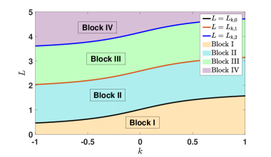
Fig. 1. $k-L$ plane is seperated by marginal curves determined by $\mathcal{A}_{a,b,\lambda}$ for different cases.

The calculation of $\mathcal{A}_{a,b,\lambda}$ is provided in Appendix A. It is worth noting that $N_{a,b,\lambda}$ is a constant within each block as per Lemma 3.2. Moreover, for $L=0$, we have $F_{a,b,\lambda,k,L}(\sigma)=k-1\neq 0$ for $k\in(-1,1)$, which implies that $N_{a,b,\lambda}(k,0)=0$. As a result, $N_{a,b,\lambda}({\rm Block~{}I})=0$, and the corresponding system (1.2) (1.3) with $(k,L)$ in Block I is exponentially stable.

We can further demonstrate that if a point $(k,L)$ moves from one block to a block above it, then $N_{a,b,\lambda}$ increases by $1$. Therefore, for any point $(k,L)$ in a block other than Block I, the system (1.2) (1.3) possesses at least one eigenvalue in $\overline{\mathbb{C}}_{+}$ and cannot be exponentially stable.

Lemma 3.3.

For $(k_{0},L_{0})\in\mathcal{A}_{a,b,\lambda}$, there exists $\varepsilon>0$, such that

$$N_{a,b,\lambda}(k_{0},L_{0}+\varepsilon)=N_{a,b,\lambda}(k_{0},L_{0}-\varepsilon)+1.$$

Proof of Lemma 3.3.

From Appendix A, if $(k_{0},L_{0})\in\mathcal{A}_{a,b,\lambda}$, we have:

$$F_{a,b,\lambda,k_{0},L_{0}}(0)=0,$$

with

$$F_{a,b,\lambda,k,L}(\sigma)=(k-1)\cosh(\eta L)-\big{[}(k+1)\frac{\lambda+1}{2\lambda}\sigma+(\frac{kb}{\lambda}+a)\big{]}\frac{\sinh(\eta L)}{\eta}.$$

Denote $\sigma_{0}=0$ and the corresponding $\eta$ is denoted by $\eta_{0}$, from Eq.(3.10),

$$\eta_{0}\coth(\eta_{0}L_{0})=\frac{(\frac{kb}{\lambda}+a)}{(k-1)}.$$ (3.27)

Denote

$$H_{a,b,\lambda,k}(\sigma,L)\triangleq(k-1)\cosh(\eta L)-\big{[}(k+1)\frac{\lambda+1}{2\lambda}\sigma+(\frac{kb}{\lambda}+a)\big{]}\frac{\sinh(\eta L)}{\eta},$$

with

$$\eta^{2}=\frac{(\lambda+1)^{2}\sigma^{2}-4\lambda ab}{4\lambda^{2}},$$

and

$$\widetilde{H}_{a,b,\lambda,k}(\eta,\sigma,L)\triangleq(k-1)\cosh(\eta L)-\big{[}(k+1)\frac{\lambda+1}{2\lambda}\sigma+(\frac{kb}{\lambda}+a)\big{]}\frac{\sinh(\eta L)}{\eta}.$$

• If $ab\neq 0$, $\eta_{0}\neq 0$, at point $(\sigma_{0},L_{0})$, we have

  $$\frac{\partial\eta}{\partial\sigma}\bigg{|}_{(\sigma,L)=(0,L_{0})}=\frac{(\lambda+1)^{2}}{4\lambda^{2}}\frac{\sigma}{\eta}=0.$$

  The partial diffierential derivative of $H_{a,b,\lambda,k}(\sigma,L)$ with respect to $\sigma$ is

  $$\frac{\partial H_{a,b,\lambda,k}}{\partial\sigma}\bigg{|}_{(\sigma,L)=(0,L_{0})}=\frac{\partial\widetilde{H}_{a,b,\lambda,k}}{\partial\eta}\cdot\frac{\partial\eta}{\partial\sigma}+\frac{\partial\widetilde{H}_{a,b,\lambda,k}}{\partial\sigma}=\frac{\partial\widetilde{H}_{a,b,\lambda,k}}{\partial\sigma}=-(k+1)\frac{\lambda+1}{2\lambda}\frac{\sinh(\eta_{0}L_{0})}{\eta_{0}}\neq 0.$$

  Notice $\eta_{0}$ is a pure imaginary number ($ab>0$) or a real number ($ab<0$), from Eq.(3.27), the partial diffierential derivative of $H_{a,b,\lambda,k}(\sigma,L)$ with respect to $L$ is:

  $$\frac{\partial H_{a,b,\lambda,k}}{\partial L}\bigg{|}_{(\sigma,L)=(0,L_{0})}= \bigg{[}(k-1)\sinh(\eta_{0}L_{0})-(\frac{kb}{\lambda}+a)\frac{\cosh(\eta_{0}L_{0})}{\eta_{0}}\bigg{]}\eta_{0}$$

  $$= \bigg{[}(k-1)\sinh(\eta_{0}L_{0})-(k-1)\frac{\cosh^{2}(\eta_{0}L_{0})}{\sinh(\eta_{0}L_{0})}\bigg{]}\eta_{0}$$

  $$= -\frac{(k-1)\eta_{0}}{\sinh(\eta_{0}L_{0})}.$$

  Using the Implicit Function Theorem 2.2, there exists an implicit function $\sigma(L)$ defined on $(L_{0}-\epsilon,L_{0}+\epsilon)$ for small sufficiently $\epsilon>0$ such that

  $$H_{a,b,\lambda,k}(\sigma(L),L)=0,\sigma(L_{0})=0,$$

  and $\sigma^{\prime}(L)=-\bigg{(}\frac{\partial H_{a,b,\lambda,k}}{\partial L}\bigg{)}/\bigg{(}\frac{\partial H_{a,b,\lambda,k}}{\partial\sigma}\bigg{)}$. More precisely,

  $$\sigma^{\prime}(L_{0})=\frac{-2\lambda(k-1)}{(\lambda+1)(k+1)}\cdot\frac{\eta_{0}^{2}}{\sinh^{2}(\eta_{0}L_{0})}>0.$$

  The last inequality is obtained by $\frac{\eta_{0}}{\sinh(\eta_{0}L_{0})}\in\mathbb{R}\backslash\{0\}$. Then we finish the proof with $ab\neq 0$.

• If $ab=0$, we have the following characteristic equation

  $$(k-1)\cosh(\eta L)-\big{(}(k+1)\frac{\lambda+1}{2\lambda}\sigma+(\frac{kb}{\lambda}+a)\big{)}\frac{\sinh(\eta L)}{\eta}=0,$$ (3.28)

  with $\eta=\frac{(\lambda+1)\sigma}{2\lambda}$.

  At point $(\sigma_{0},L_{0})$, we obtain

  $$(k-1)-(\frac{kb}{\lambda}+a)L_{0}=0.$$

  Moreover,

  $$\frac{\partial\eta}{\partial\sigma}|_{(\sigma,L)=(0,L_{0})}=\frac{\lambda+1}{2\lambda}.$$

  Since $\cosh(\eta L)$ and $\frac{\sinh(\eta L)}{\eta}$ are analytic functions with respect to $\eta^{2}$, we obtain

  $$\frac{\partial\widetilde{H}_{a,b,\lambda,k}}{\partial\eta}|_{(\eta,\sigma,L)=(0,0,L_{0})}=0.$$

  Thus,

  $$\frac{\partial H_{a,b,\lambda,k}}{\partial\sigma}|_{(\sigma,L)=(0,L_{0})}=\frac{\partial\widetilde{H}_{a,b,\lambda,k}}{\partial\eta}\cdot\frac{\partial\eta}{\partial\sigma}+\frac{\partial\widetilde{H}_{a,b,\lambda,k}}{\partial\sigma}$$

  $$= -(k+1)\frac{\lambda+1}{2\lambda}\frac{\sinh(\eta_{0}L_{0})}{\eta_{0}}=-(k+1)\frac{\lambda+1}{2\lambda}L_{0}\neq 0.$$

  The partial diffierential derivative of $H_{a,b,\lambda,k}(\sigma,L)$ with respect to $L$ is

  $$\frac{\partial H_{a,b,\lambda,k}}{\partial L}|_{(\sigma,L)=(0,L_{0})}=-(\frac{kb}{\lambda}+a).$$

  Using the Implicit Function Theorem 2.2, there exists an implicit function $\sigma(L)$ defined on $(L_{0}-\epsilon,L_{0}+\epsilon)$ for small sufficiently $\epsilon>0$ such that

  $$H_{a,b,\lambda,k}(\sigma(L),L)=0,\sigma(L_{0})=0,$$

  and $\sigma^{\prime}(L)=-\bigg{(}\frac{\partial H_{a,b,\lambda,k}}{\partial L}\bigg{)}/\bigg{(}\frac{\partial H_{a,b,\lambda,k}}{\partial\sigma}\bigg{)}$. More precisely,

  $$\sigma^{\prime}(L_{0})=-\frac{2\lambda(k-1)}{(\lambda+1)(k+1)L_{0}^{2}}>0.$$

  Then we finish the proof of $ab=0$.

∎

Proof of Theorem 1.1

Lemma 3.3 gives us a way to determine $N_{a,b,\lambda}$ for each block. For example, for the case $ab>0$, the $k-L$ plane is seperated into infinitely blocks by marginal curves determined by $\mathcal{A}_{a,b,\lambda}$ (see Fig. 2). Thus, we know that $N_{a,b,\lambda}({\rm Block~{}I})=0,\ N_{a,b,\lambda}({\rm Block~{}II})=1,\ N_{a,b,\lambda}({\rm Block~{}III})=2,\ N_{a,b,\lambda}({\rm Block~{}IV})=3$ and so on. For the case $a>0,b=0$, there are no marginal curves (See Fig. 2). Thus, we know that for all the point $(k,L)\in(-1,1)\times[0,+\infty)$, we have $N_{a,b,\lambda}(k,L)=0$.

Fig. 2. $k-L$ plane is seperated by marginal curves determined by $\mathcal{A}_{a,b,\lambda}$ for different cases.

Thus we know that the stability region is the block at the bottom which contains $\{(k,0)|k\in(-1,1)\}$. Denote $D(a,b,\lambda)$ is the block that contains $\{(k,0)|k\in(-1,1)\}$, we obtain

$$L_{c}(a,b,\lambda)=\max\{L|(k,L)\in D(a,b,\lambda)\}.$$

Moreover, if $\mathcal{A}_{a,b,\lambda}=\emptyset$, for any $L>0$, the corresponding system (1.2) (1.3) with $(k,L)$ is exponentially stable with $L_{c}\triangleq+\infty$ that is defined in Theorem 1.1. More precisely, from the calculation in Appendix A, we obtain

$$L_{c}=\begin{cases}\sqrt{\frac{\lambda}{ab}}\pi,\quad&\text{if}\ a>0,b>0.\\ \sqrt{\frac{\lambda}{ab}}\arccot(\frac{b-\lambda a}{2\sqrt{\lambda ab}}),\quad&\text{if}\ a<0,b<0.\\ \sqrt{\frac{-\lambda}{ab}}\coth^{-1}(\frac{b-\lambda a}{2\sqrt{-\lambda ab}}),\quad&\text{if}\ -\lambda a>b>0.\\ -\frac{2}{a},\quad&\text{if}\ b=0,a<0.\\ +\infty,\quad&\text{if else.}\end{cases}$$ (3.29)

4. Numerical Simulations

In this section we present some numerical simulations generated with MATLAB of upwind scheme with implicit methods for the system (1.2) (1.3). We adopt the finite difference method in both the time and the space domain, which can be written as follows. The grid size $N=100$ and the time step $\Delta t=2L/N$ are used.

$$\begin{cases}\frac{u_{j}^{n+1}-u_{j}^{n}}{\Delta t}+\frac{u_{j}^{n+1}-u_{j-1}^{n+1}}{\Delta x}+av_{j}^{n+1}=0,\quad&j=1,...,N;n=0,...,\frac{T}{\Delta t},\\ \frac{v_{j}^{n+1}-v_{j}^{n}}{\Delta t}-\lambda\frac{v_{j+1}^{n+1}-v_{j}^{n+1}}{\Delta x}+bu_{j}^{n+1}=0,\quad&j=0,...,N-1;n=0,...,\frac{T}{\Delta t},\\ u_{0}^{n}=kv_{0}^{n},\quad&n=0,...,\frac{T}{\Delta t},\\ u_{N}^{n}=v_{N}^{n},\quad&n=0,...,\frac{T}{\Delta t}.\par\end{cases}$$

Here $u_{j}^{n}$ and $v_{j}^{n}$ provide an approximation of $y_{1}(x_{j},t_{n})$ and $y_{2}(x_{j},t_{n})$, respectively. The initial conditions are chosen as

$$\begin{cases}y_{1}(0,x)=x+\sin^{2}x,\\ y_{2}(0,x)=\frac{L+\sin^{2}L}{L+L^{2}}(x^{2}+x).\end{cases}$$

Energy is measured in the $L_{2}$-norm for

$$E_{t}\triangleq\int_{0}^{L}[y_{1}(t,x)^{2}+y_{2}(t,x)^{2}]{\rm d}x.$$

We choose four triple $(a,b,\lambda)=(1,1,1),(-1,-2,1),(0,1,1),(-1,0,1)$. For each triple value of $(a,b,\lambda)$, we numerically implement system (1.2) for the parameter $(k,L)\in(-1,1)\times(0,3)$. As shown in Fig. 3, the analytical creteria for stability region established in Section 3 can be confirmed by our numerical simulations. Specially, for $a=-1,b=-2,\lambda=1,L=0.9$, Fig. 3 shows that the system will be stabilized only when the coupling gain $k\in(-1,k_{*})$ for $k_{*}\approx-0.23$. Numerical confirmation is shown in Fig. 4. For different values of coupling gain $k$, the energy converges or diverges exponentially with different rates.

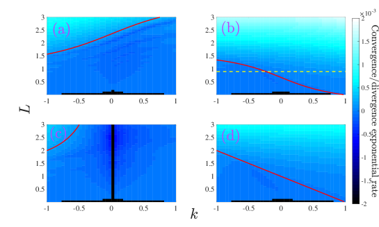
Fig. 3. Red curves are depicted by the analytical results according to Appendix.A, below which are the stability region for $k,L$. The colors represent the exponential rates of the convergence or divergence of the trajectory numerically generated by Eq.(1.2). The parameters are (a) $a=1,b=1,\lambda=1$ (b) $a=-1,b=-2,\lambda=1$ (c) $a=0,b=1,\lambda=1$ (d) $a=-1,b=0,\lambda=1$. Yellow dashed line in (b) represents $L=0.9$, which will be investigated more clearly in Fig. 4.

Fig. 4. For different values of coupling gain $k$, the energy $E_{t}$ converges or diverges exponentially with different rates. The parameters are $a=-1,b=-2,\lambda=1,L=0.9$.

5. Backstepping control

In this section, we want to use Backstepping method combined with the observer design to stabilize the system with the case that cannot be stabilized by the proportional feedback control. We first make a scaling of space variable $x\rightarrow L-x$, then the control could be on the right side and the boundary condition be on the left. Theorem 1.1 can apply to the following system:

$$\begin{cases}\partial_{t}y_{1}-\partial_{x}y_{1}+ay_{2}=0,\quad&(t,x)\in(0,+\infty)\times(0,L),\\ \partial_{t}y_{2}+\lambda\partial_{x}y_{2}+by_{1}=0,\quad&(t,x)\in(0,+\infty)\times(0,L),\\ y_{2}(t,0)=y_{1}(t,0),\quad&t\in(0,+\infty),\\ y_{1}(t,L)=U(t),\quad&t\in(0,+\infty).\end{cases}$$ (5.1)

The output is

$$Y(t)=y_{2}(t,L).$$ (5.2)

Applying the results in Anfinsen et al.[2], we design the following observer:

$$\begin{cases}\partial_{t}\hat{y}_{1}-\partial_{x}\hat{y}_{1}+a\hat{y}_{2}=\Gamma_{1}(x)(Y(t)-\hat{y}_{2}(t,L)),\quad(t,x)\in(0,+\infty)\times(0,L),\\ \partial_{t}\hat{y}_{2}+\lambda\partial_{x}\hat{y}_{2}+b\hat{y}_{1}=\Gamma_{2}(x)(Y(t)-\hat{y}_{2}(t,L)),\quad(t,x)\in(0,+\infty)\times(0,L),\\ \hat{y}_{2}(t,0)=\hat{y}_{1}(t,0),\quad t\in(0,+\infty),\\ \hat{y}_{1}(t,L)=U(t),\quad t\in(0,+\infty),\end{cases}$$ (5.3)

with $\Gamma_{1}(x),\Gamma_{2}(x)$ are injection gains to be designed.

We have the following proposition:

Proposition 5.1.

Suppose the system (5.1) and the observer (5.3) with $\lambda,a,b\in\mathbb{R}$, $T_{opt1}\triangleq\frac{(\lambda+1)}{\lambda}L$. There exists suitable injection designs $\Gamma_{1}(x),\Gamma_{2}(x)$ such that for all $t>T_{opt1}$, we have:

$$\begin{cases}y_{1}(t,{x})=\hat{y}_{1}(t,x),\quad(t,x)\in[T_{opt1},+\infty)\times[0,L],\\ y_{2}(t,{x})=\hat{y}_{2}(t,x),\quad(t,x)\in[T_{opt1},+\infty)\times[0,L].\end{cases}$$ (5.4)

Proof of Proposition 5.1.

The state estimation errors $\widetilde{y}_{1}\triangleq y_{1}-\hat{y}_{1},\widetilde{y}_{2}\triangleq y_{2}-\hat{y}_{2}$ satisfy the dynamics:

$$\begin{cases}\partial_{t}\widetilde{y}_{1}-\partial_{x}\widetilde{y}_{1}+a\widetilde{y}_{2}=-\Gamma_{1}(x)\widetilde{y}_{2}(L),\quad&(t,x)\in(0,+\infty)\times(0,L),\\ \partial_{t}\widetilde{y}_{2}+\lambda\partial_{x}\widetilde{y}_{2}+b\widetilde{y}_{1}=-\Gamma_{2}(x)\widetilde{y}_{2}(L),\quad&(t,x)\in(0,+\infty)\times(0,L),\\ \widetilde{y}_{2}(t,0)=\widetilde{y}_{1}(t,0),\quad&t\in(0,+\infty),\\ \widetilde{y}_{1}(t,L)=0,\quad&t\in(0,+\infty).\end{cases}$$ (5.5)

Design the backstepping transformation:

$$\begin{cases}\widetilde{y}_{1}(t,x)=\alpha(t,x)+\int_{x}^{L}P^{1}(x,\xi)\beta(t,\xi){\rm d}\xi,\\ \widetilde{y}_{2}(t,x)=\beta(t,x)+\int_{x}^{L}P^{2}(x,\xi)\beta(t,\xi){\rm d}\xi,\end{cases}$$ (5.6)

which makes system (5.5) become the target system as follows.

$$\begin{cases}\partial_{t}\alpha-\partial_{x}\alpha+\int_{x}^{L}Q^{1}(x,\xi)\alpha(\xi){\rm d}\xi=0,\quad&(t,x)\in(0,+\infty)\times(0,L),\\ \partial_{t}\beta+\lambda\partial_{x}\beta+\int_{x}^{L}Q^{2}(x,\xi)\alpha(\xi){\rm d}\xi+b\alpha=0,\quad&(t,x)\in(0,+\infty)\times(0,L),\\ \alpha(t,0)=\beta(t,0),\quad&t\in(0,+\infty),\\ \alpha(t,L)=0,\quad&t\in(0,+\infty).\end{cases}$$ (5.7)

The proof of existence of $Q^{1},Q^{2},P^{1},P^{2}$ can be found in [2, Section B]. The solution of target system (5.7) will vanish in finite time for $t>T_{opt1}$. If we denote by $\Gamma_{1}(x)\triangleq\lambda P^{1}(x,L),\Gamma_{2}(x)\triangleq\lambda P^{2}(x,L)$, by the transformation (5.6), we obtain that the solution $[\tilde{y_{1}},\tilde{y_{2}}]^{\rm T}$ of Eq.(5.5) will vanish when $t>T_{opt1}$. ∎

It follows from Proposition 5.1 that the right side of Eq.(5.3) vanishes when $t>T_{opt1}$, which makes it become a homogeneous linear hyperbolic system. By [21, Section 2.2, Section 2.3], we know that there exists an invertible backstepping transformation

$$\begin{cases}z(t,x)=\hat{y}_{1}(t,x)-\int_{0}^{x}[K^{11}(x,\xi)\hat{y}_{1}(t,\xi)+K^{12}(x,\xi)\hat{y}_{2}(t,\xi)]{\rm d}\xi,\\ w(t,x)=\hat{y}_{2}(t,x)-\int_{0}^{x}[K^{21}(x,\xi)\hat{y}_{1}(t,\xi)+K^{22}(x,\xi)\hat{y}_{2}(t,\xi)]{\rm d}\xi,\end{cases}$$ (5.8)

with its inverse transformation

$$\begin{cases}\hat{y}_{1}(t,x)=z(t,x)+\int_{0}^{x}[L^{11}(x,\xi)z(t,\xi)+L^{12}(x,\xi)w(t,\xi)]{\rm d}\xi,\\ \hat{y}_{2}(t,x)=w(t,x)+\int_{0}^{x}[L^{21}(x,\xi)z(t,\xi)+L^{22}(x,\xi)w(t,\xi)]{\rm d}\xi,\end{cases}$$ (5.9)

which transforms system (5.3) into the target system as follows.

$$\begin{cases}\partial_{t}z-\partial_{x}z=0,\quad&(t,x)\in(T_{opt1},+\infty)\times(0,L),\\ \partial_{t}w+\lambda\partial_{x}w=g(x)w(t,0),\quad&(t,x)\in(T_{opt1},+\infty)\times(0,L),\\ w(t,0)=z(t,0),\quad&t\in(T_{opt1},+\infty),\\ z(t,L)=0,\quad&t\in(T_{opt1},+\infty).\end{cases}$$ (5.10)

From transformation (5.9) evaluated at $x=L$, noting that $z(t,L)\equiv 0$, we obtain the following feedback control laws for the system (5.3)

$$U(t)\triangleq\int_{0}^{L}[L^{11}(L,\xi)z(t,\xi)+L^{12}(L,\xi)w(t,\xi)]{\rm d}\xi.$$

This yields that $\hat{y}_{1},\hat{y}_{2}$ vanishes in finite time $t\geq T_{opt}\triangleq T_{opt1}+T_{opt2}$ with $T_{opt1}=T_{opt2}=\dfrac{(\lambda+1)L}{\lambda}.$ Thus we get the main theorem in this section.

Theorem 5.1.

There exists a boundary feedback control law $U(t)$ for the system (5.1) with $\lambda,a,b\in\mathbb{R}$ such that, for every $Y_{0}\in L^{2}(0,L)$, the solution $Y\in C^{0}([0,+\infty);L^{2}(0,L))$ to (5.1) satisfies $Y(t)=0,\forall t\geq T_{opt},$ where $T_{opt}=\frac{2(\lambda+1)}{\lambda}L$.

Remark 5.1.

Proposition 5.1 and Theorem 5.1 have designed boundary feedback controls that stablize the cases which cannot be stabilized by the proportional boundary feedback control mentioned in Theorem 1.1.

Remark 5.2.

For the following system:

$$\begin{cases}\partial_{t}y_{1}-\lambda(x)\partial_{x}y_{1}+a(x)y_{2}=0,\quad&(t,x)\in(0,+\infty)\times(0,L),\\ \partial_{t}y_{2}+\mu(x)\partial_{x}y_{2}+b(x)y_{1}=0,\quad&(t,x)\in(0,+\infty)\times(0,L),\\ y_{2}(t,0)=y_{1}(t,0),\quad&t\in(0,+\infty),\\ y_{1}(t,L)=U(t),\quad&t\in(0,+\infty).\end{cases}$$ (5.11)

with $\lambda(x),\mu(x)\in C^{1}([0,L]),a(x),b(x)\in C^{0}([0,1])$ are known functions that satisfied $\lambda(x),\mu(x)>0$ and $k\in\mathbb{R}$.

The basic ideas of designing the observer in Proposition 5.1 and the backstepping control in Theorem 5.1 can be applied to this system. Therefore, the system could be stabilized to zero in finite time by a boundary control $U(t)$ depending on $y_{2}(\tau,L)(\tau\in(0,t))$.

Appendix A Calculation on $\mathcal{A}_{a,b,\lambda}$

Recall that the characteristic equation (3.10) is

$$(k-1)\cosh(\eta L)-\big{[}(k+1)\frac{\lambda+1}{2\lambda}\sigma+(\frac{kb}{\lambda}+a)\big{]}\frac{\sinh(\eta L)}{\eta}=0.$$

with

$$\eta^{2}=\frac{(\lambda+1)^{2}\sigma^{2}-4\lambda ab}{4\lambda^{2}}.$$

and the definition of $\mathcal{A}_{a,b,\lambda}$ is

$$\mathcal{A}_{a,b,\lambda}:=\big{\{}(k,L)||k|<1,L\geq 0,\ \text{there exists}\ \beta\in\mathbb{R}\ \text{such that}\ F_{a,b,\lambda,k,L}(\mathrm{i}\beta)=0\big{\}},$$

First, if $L=0$, we have $F_{a,b,\lambda,k,L}(\sigma)=k-1\neq 0$ for $k\in(-1,1)$, which means

$$(k,0)\not\in\mathcal{A}_{a,b,\lambda}.$$ (A.1)

We discuss $\mathcal{A}_{a,b,\lambda}$ with $(k,L)\in(-1,1)\times(0,+\infty)$. We first observe that if $\sigma=\mathrm{i}\beta$, we have

$$\eta^{2}\in\mathbb{R},\ \cosh(\eta L)\in\mathbb{R},\ \frac{\sinh(\eta L)}{\eta}\in\mathbb{R}.$$

Thus, the imaginary part of Eq.(3.10) is:

$$(k+1)\frac{\lambda+1}{2\lambda}\beta\frac{\sinh(\eta L)}{\eta}=0,$$ (A.2)

and the real part of Eq.(3.10) is:

$$(k-1)\cosh(\eta L)-(\frac{kb}{\lambda}+a)\frac{\sinh(\eta L)}{\eta}=0.$$ (A.3)

If $\frac{\sinh(\eta L)}{\eta}=0$ (motivated by Eq.(A.2)), the left side of Eq.(A.3) is $k-1\neq 0$, thus $\frac{\sinh(\eta L)}{\eta}\neq 0$.

From Eq.(A.2), we obtain

$$\beta=0.$$

Therefore,

$$\mathcal{A}_{a,b,\lambda}=\big{\{}(k,L)||k|<1,L>0,F_{a,b,\lambda,k,L}(0)=0\big{\}},$$

and the characteristic equation can be simplified:

$$(k-1)\cosh(\eta L)-(\frac{kb}{\lambda}+a)\frac{\sinh(\eta L)}{\eta}=0,$$ (A.4)

with

$$\eta^{2}=-\frac{ab}{\lambda}.$$

We now divide into three cases:

• $ab=0$, the corresponding $\eta=0$. Eq.(A.4) yields:

  $$(k-1)-(\frac{kb}{\lambda}+a)L=0.$$

  Define $L_{k}\triangleq\frac{k-1}{\frac{kb}{\lambda}+a}$, we obtain

  $$\mathcal{A}_{a,b,\lambda}=\begin{cases}\big{\{}(k,L_{k})|k\in(-1,0]\big{\}},\quad&\text{if}\ a=0,b>0.\\ \big{\{}(k,L_{k})|k\in[0,1)\big{\}},\quad&\text{if}\ a=0,b<0.\\ \emptyset,\quad&\text{if}\ a\geq 0,b=0.\\ \big{\{}(k,L_{k})|k\in(-1,1)\big{\}},\quad&\text{if}\ a<0,b=0.\end{cases}$$ (A.5)

  

  

  

  

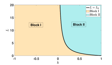
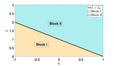
  Fig. 5. $k-L$ plane is seperated by marginal curves determined by $\mathcal{A}_{a,b,\lambda}$ for the case $ab=0$. Black marginal curves are determined by Eq.(A.5). The parameters are (a) $a=0,b=1,\lambda=1$,(b) $a=0,b=-1,\lambda=1$, (c) $a=-1,b=0,\lambda=1$, (d) $a=1,b=0,\lambda=1$.

  That is

  $$L_{c}=\begin{cases}+\infty,\quad&\text{if}\ a=0.\\ +\infty,\quad&\text{if}\ a\geq 0,b=0.\\ L_{-1}=-\frac{2}{a},\quad&\text{if}\ a<0,b=0.\end{cases}$$ (A.6)

• $ab>0$, Eq.(A.4) yields:

  $$(k-1)\cos(\sqrt{\frac{ab}{\lambda}})-(\frac{kb}{\lambda}+a)\frac{\sin(\sqrt{\frac{ab}{\lambda}})}{\sqrt{\frac{ab}{\lambda}}}=0.$$

  It can be written as

  $$\cot(\sqrt{\frac{ab}{\lambda}}L)=\frac{\frac{kb}{\lambda}+a}{(k-1)\sqrt{\frac{ab}{\lambda}}}.$$

  We define

  $$L_{k,n}\triangleq\sqrt{\frac{\lambda}{ab}}\bigg{(}\arccot\big(\frac{\frac{kb}{\lambda}+a}{(k-1)\sqrt{\frac{ab}{\lambda}}}\big{missing})+n\pi\bigg{)}\ (n\in\mathbb{N}).$$ (A.7)

  Then we obtain

  $$\mathcal{A}_{a,b,\lambda}=\big{\{}(k,L_{k,n})|k\in(-1,1)\big{\}}.$$

  

  

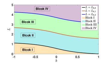
  Fig. 6. $k-L$ plane is seperated by marginal curves determined by $\mathcal{A}_{a,b,\lambda}$ for the case $ab>0$. Black marginal curves are determined by Eq.(A.7). The parameters are (a) $a=-1,b=-4,\lambda=1$,(b) $a=1,b=4,\lambda=1$.

  That is,

  $$L_{c}=\begin{cases}L_{1,0}=\sqrt{\frac{\lambda}{ab}}\pi,\quad&\text{if}\ a,b>0.\\ L_{-1,0}=\sqrt{\frac{\lambda}{ab}}\arccot(\frac{b-\lambda a}{2\sqrt{\lambda ab}}),\quad&\text{if}\ a,b<0.\end{cases}$$ (A.8)

• $ab<0$, Eq.(A.4) yields:

  $$\coth(\sqrt{-\frac{ab}{\lambda}}L)=\frac{\frac{kb}{\lambda}+a}{(k-1)\sqrt{-\frac{ab}{\lambda}}}.$$

  Only if $\frac{\frac{kb}{\lambda}+a}{(k-1)\sqrt{-\frac{ab}{\lambda}}}>1$ the marginal curves exists, which can be defined by

  $$L_{k}\triangleq\sqrt{-\frac{\lambda}{ab}}\coth^{-1}(\frac{\frac{kb}{\lambda}+a}{(k-1)\sqrt{-\frac{ab}{\lambda}}})>0.$$ (A.9)

  More precisely, let

  $$h(k)\triangleq\frac{\frac{kb}{\lambda}+a}{(k-1)\sqrt{-\frac{ab}{\lambda}}},$$

  which is continuous in $(k,L)\in(-1,1)\times(0,+\infty)$. Denote by

  $$k_{1}\triangleq\frac{-\lambda a-\sqrt{-\lambda ab}}{b-\sqrt{-\lambda ab}}=\sqrt{\dfrac{-\lambda a}{b}}{\rm Sgn}(a),$$

  with $h(k_{1})=1$.

  • $-\lambda a\geq b>0$, $h^{\prime}(k)>0$. The range of $h(k)$ is $(h(-1),+\infty)$ with $h(-1)>1$.

    $$\mathcal{A}_{a,b,\lambda}=\big{\{}(k,L_{k})|k\in(-1,1)\big{\}}.$$

  • $0>-\lambda a>b$, $h^{\prime}(k)>0$. The range of $h(k)$ is $(h(-1),+\infty)$ with $h(-1)<-1$.

    $$\mathcal{A}_{a,b,\lambda}=\big{\{}(k,L_{k})|k\in(k_{1},1)\big{\}}.$$

  • $b>-\lambda a>0$, $h^{\prime}(k)<0$. The range of $h(k)$ is $(-\infty,h(-1))$ with $h(-1)>1$.

    $$\mathcal{A}_{a,b,\lambda}=\big{\{}(k,L_{k})|k\in(-1,k_{1})\big{\}}.$$

  • $0>b\geq-\lambda a$, $h^{\prime}(k)<0$. The range of $h(k)$ is $(-\infty,h(-1))$ with $h(-1)<-1$. We obtain $L_{k}<0$ for $k\in(-1,1)$.

    $$\mathcal{A}_{a,b,\lambda}=\emptyset.$$

  

  

  

  

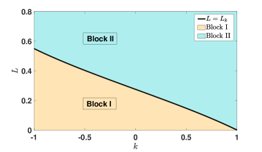
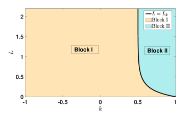
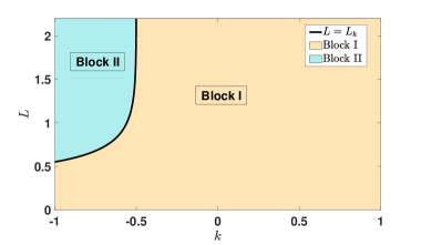
  Fig. 7. $k-L$ plane is seperated into several blocks by marginal curves determined by $\mathcal{A}_{a,b,\lambda}$ for the case $ab<0$. Black marginal curves are determined by Eq.(A.9). The parameters are (a) $a=-4,b=1,\lambda=1$,(b) $a=1,b=-4,\lambda=1$, (c) $a=-1,b=4,\lambda=1$, (d) $a=4,b=-1,\lambda=1$.

  It is not difficult to obtain while $ab<0$:

  $$L_{c}=\begin{cases}L_{-1}=\sqrt{-\frac{\lambda}{ab}}\coth^{-1}(\frac{b-\lambda a}{2\sqrt{-\lambda ab}}),\quad&\text{if}\ -\lambda a>b>0.\\ +\infty,\quad&\text{else}.\end{cases}$$

We finish the discuss on the set $\mathcal{A}_{a,b,\lambda}$.

References

[1]
Fabio Ancona and Andrea Marson.
Asymptotic stabilization of systems of conservation laws by controls
acting at a single boundary point.
In Control methods in PDE-dynamical systems, volume 426 of
Contemp. Math., pages 1–43. Amer. Math. Soc., Providence, RI, 2007.
[2]
Henrik Anfinsen and Ole Morten Aamo.
Adaptive stabilization of linear hyperbolic systems with
an unknown boundary parameter from collocated sensing and control.
IEEE Transactions on Automatic Control, 62(12):6237–6249,
2017.
[3]
Henrik Anfinsen and Ole Morten Aamo.
Adaptive control of linear hyperbolic systems.
Automatica J. IFAC, 87:69–82, 2018.
[4]
Georges Bastin and Jean-Michel Coron.
On boundary feedback stabilization of non-uniform linear
hyperbolic systems over a bounded interval.
Systems Control Lett., 60(11):900–906, 2011.
[5]
Georges Bastin and Jean-Michel Coron.
Stability and boundary stabilization of 1-D hyperbolic
systems, volume 88 of Progress in Nonlinear Differential Equations and
their Applications.
Birkhäuser/Springer, [Cham], 2016.
Subseries in Control.
[6]
Georges Bastin, Jean-Michel Coron, and Simona Oana Tamasoiu.
Stability of linear density-flow hyperbolic systems under PI
boundary control.
Automatica J. IFAC, 53:37–42, 2015.
[7]
Alberto Bressan and Giuseppe Maria Coclite.
On the boundary control of systems of conservation laws.
SIAM J. Control Optim., 41(2):607–622, 2002.
[8]
Jean-Michel Coron.
Control and nonlinearity, volume 136 of Mathematical
Surveys and Monographs.
American Mathematical Society, Providence, RI, 2007.
[9]
Jean-Michel Coron and Georges Bastin.
Dissipative boundary conditions for one-dimensional quasi-linear
hyperbolic systems: Lyapunov stability for the -norm.
SIAM J. Control Optim., 53(3):1464–1483, 2015.
[10]
Jean-Michel Coron, Georges Bastin, and Brigitte d’Andréa Novel.
Dissipative boundary conditions for one-dimensional nonlinear
hyperbolic systems.
SIAM J. Control Optim., 47(3):1460–1498, 2008.
[11]
Jean-Michel Coron, Brigitte d’Andréa Novel, and Georges Bastin.
A strict Lyapunov function for boundary control of hyperbolic
systems of conservation laws.
IEEE Trans. Automat. Control, 52(1):2–11, 2007.
[12]
Jean-Michel Coron, Sylvain Ervedoza, Shyam Sundar Ghoshal, Olivier Glass, and
Vincent Perrollaz.
Dissipative boundary conditions for hyperbolic systems
of conservation laws for entropy solutions in BV.
J. Differential Equations, 262(1):1–30, 2017.
[13]
Jean-Michel Coron, Long Hu, Guillaume Olive, and Peipei Shang.
Boundary stabilization in finite time of one-dimensional linear
hyperbolic balance laws with coefficients depending on time and space.
J. Differential Equations, 271:1109–1170, 2021.
[14]
Ababacar Diagne, Georges Bastin, and Jean-Michel Coron.
Lyapunov exponential stability of 1-D linear hyperbolic systems of
balance laws.
Automatica J. IFAC, 48(1):109–114, 2012.
[15]
Markus Dick, Martin Gugat, and Günter Leugering.
Classical solutions and feedback stabilization for the gas flow in a
sequence of pipes.
Netw. Heterog. Media, 5(4):691–709, 2010.
[16]
Markus Dick, Martin Gugat, and Günter Leugering.
A strict -Lyapunov function and feedback stabilization for
the isothermal Euler equations with friction.
Numer. Algebra Control Optim., 1(2):225–244, 2011.
[17]
Klaus Fritzsche and Hans Grauert.
From holomorphic functions to complex manifolds, volume 213 of
Graduate Texts in Mathematics.
Springer-Verlag, New York, 2002.
[18]
Martin Gugat and Markus Dick.
Time-delayed boundary feedback stabilization of the isothermal
Euler equations with friction.
Math. Control Relat. Fields, 1(4):469–491, 2011.
[19]
Martin Gugat and Stephan Gerster.
On the limits of stabilizability for networks of strings.
Systems Control Lett., 131:104494, 10, 2019.
[20]
Martin Gugat, Günter Leugering, and Ke Wang.
Neumann boundary feedback stabilization for a nonlinear wave
equation: a strict -Lyapunov function.
Math. Control Relat. Fields, 7(3):419–448, 2017.
[21]
Long Hu, Rafael Vazquez, Florent Di Meglio, and Miroslav Krstic.
Boundary exponential stabilization of 1-dimensional inhomogeneous
quasi-linear hyperbolic systems.
SIAM J. Control Optim., 57(2):963–998, 2019.
[22]
Tatsien Li.
Global classical solutions for quasilinear hyperbolic systems,
volume 32 of RAM: Research in Applied Mathematics.
Masson, Paris; John Wiley & Sons, Ltd., Chichester, 1994.
[23]
Tatsien Li, Bopeng Rao, and Zhiqiang Wang.
Exact boundary controllability and observability for first order
quasilinear hyperbolic systems with a kind of nonlocal boundary conditions.
Discrete Contin. Dyn. Syst., 28(1):243–257, 2010.
[24]
Mark Lichtner.
Spectral mapping theorem for linear hyperbolic systems.
Proc. Amer. Math. Soc., 136(6):2091–2101, 2008.
[25]
Vincent Perrollaz.
Exact controllability of scalar conservation laws with an additional
control in the context of entropy solutions.
SIAM J. Control Optim., 50(4):2025–2045, 2012.
[26]
Christophe Prieur, Joseph Winkin, and Georges Bastin.
Robust boundary control of systems of conservation laws.
Math. Control Signals Systems, 20(2):173–197, 2008.
[27]
M. Slemrod.
Boundary feedback stabilization for a quasilinear wave equation.
In Control theory for distributed parameter systems and
applications (Vorau, 1982), volume 54 of Lect. Notes Control Inf.
Sci., pages 221–237. Springer, Berlin, 1983.
[28]
Abdoua Tchousso, Thibaut Besson, and Cheng-Zhong Xu.
Exponential stability of distributed parameter systems governed by
symmetric hyperbolic partial differential equations using Lyapunov’s second
method.
ESAIM Control Optim. Calc. Var., 15(2):403–425, 2009.
[29]
Cheng-Zhong Xu and Gauthier Sallet.
Exponential stability and transfer functions of processes governed by
symmetric hyperbolic systems.
ESAIM Control Optim. Calc. Var., 7:421–442, 2002.