Absorption and stationary times for the $\Lambda$-Wright-Fisher process

Abstract.

We derive stationary and fixation times for the multi-type $\Lambda$–Wright-Fisher process with and without the classic linear drift that models mutations. Our method relies on a grand coupling of the process realized through the so-called lookdown-construction. A well-known process embedded in this construction is the fixation line. We generalise the process to our setup and make use of the associated explosion times to obtain a representation of the fixation and stationary times in terms of the waiting time in a coupon collector problem.

MSC 2020. Primary:  92D15, 60J25  Secondary:  60J27, 60J90, 60J95

Keywords. $\Lambda$-Fleming-Viot, Lookdown-construction, fixation time, Waiting time coupon collector problem, Fixation line, Strong stationary time

1. Introduction

Random fluctuations in the allele frequencies of a population due to allele-independent random events is a major driver for the loss of variability within populations. In this context, it is of importance in population genetics and evolutionary biology to estimate the time until a subset of the alleles go extinct. For very large, randomly reproducing populations consisting of individuals that carry one of $(d+1)$ types, the $(d+1)$-type $\Lambda$-Wright-Fisher process can serve as a formal mathematical modeling framework. It is a jump-diffusion process on the $d$-dimensional simplex. The only parameter is a measure $\Lambda$ on $[0,1]$ that codes the offspring sizes in reproduction events. Without any deterministic drift term, all but one type eventually die out. The first time there is only one type left is called the fixation time.

For the classic Wright-Fisher diffusion, which corresponds to $\Lambda=\delta_{0}$, explicit expressions for the mean fixation time were derived by [19] (see also [8, Ch. 8] for more context). Moreover, Littler derives an expression for the probability of extinction to occur in a given order. It is well-known that for many biological systems, general measures $\Lambda$ are a more reasonable model [9] (in particular, for many marine species). In this general case, there are some results that quantify the time to absorption in the case of two types, e.g. [4, Prop. 2.29], but they are far from explicit. The current manuscript tries to fill this gap. We formulate a probabilistic framework to address the questions of absorption time and extinction in a given order based on the lookdown-constructions of [7] and a new perspective on the fixation line(s) that generalises to the situation when mutations are present (both concept will be defined in the next section). The mean fixation time decomposes essentially into two random quantities. The first is the waiting time in a coupon collector problem with non-uniform collection probabilities. The second is the mean explosion time of a fixation line ([21, 14, 15, 16]). In the special case of $\Lambda$ being a $\mathrm{Beta}\ (2-\alpha,\alpha)$ distribution with $\alpha\in(1,2)$, that is, where

(1) $$\Lambda(\textnormal{d}x)=\mathrm{Beta}(2-\alpha,\alpha)(\textnormal{d}x):=\frac{x^{1-\alpha}(1-x)^{\alpha-1}}{\Gamma(2-\alpha)\Gamma(\alpha)}{\mathds{1}_{\{[0,1]\}}}(x)\textnormal{d}x,$$

we can build on previous work by [14] to obtain explicit closed-form expressions for the mean fixation time.

Mutations can maintain genetic variation in a population. It is then of interest to estimate the time it takes for a population to reach stationarity. To incorporate mutations into the Wright-Fisher modeling framework, the SDE characteristing the process is typically augmented by an inward-pointing deterministic linear drift term. The drift term is parametrised by $\theta\in\mathbb{R}_{+}$ and a vector ${\boldsymbol{\nu}}$ from the interior of the $d$-dimensional simplex. $\theta$ codes the total rate of mutation, and the $i$th component of ${\boldsymbol{\nu}}$ corresponds to the probability of a mutation leading to type $i$. In particular, the three parameters of the model with mutation are $\Lambda$, $\theta$, and ${\boldsymbol{\nu}}$. When $\theta>0$, all the types coexist and one can study stationary times. We introduce a modified version of the lookdown-construction that is well-suited to deal with these kind of questions. Our notion of fixation line also make sense in this setting and we can therefore use essentially the same techniques to study (strong) stationary times of the process.

Our main results and the underlying ideas are stated in Section 2. In Section 3 we prove the convergence of the finite lookdown-models to the $\Lambda$-Wright-Fisher process. Results about the fixation lines are proved in Section 4. In Section 5 we prove results related to the Beta-coalescent. Finally, Section 6 contains the proofs related to the fixation and stationary times.

1.1. Notation

For $d\in\mathbb{N}$, let $[d]\coloneqq\{1,\ldots,d\}$. Vectors and sequences are in boldface. Define

$$\Delta_{d}\coloneqq\left\{{\bf{x}}=({\bf{x}}({1}),{\bf{x}}({2}),\ldots,{\bf{x}}(d))\in[0,1]^{d}:\sum_{i=1}^{d}{\bf{x}}(i)\leq 1\right\}.$$

For ${\bf{x}}\in\Delta_{d}$, we set ${\bf{x}}({d+1})=1-\sum_{i=1}^{d}{\bf{x}}({i})$. For $k\in[d+1]$, let ${\bf{e}}_{{k}}\in\mathbb{R}^{d}$ be the $k$th unit vector with the convention ${\bf{e}}_{{d+1}}=(0,\ldots,0)$. Denote by $\mathcal{M}_{f}[0,1]$ the set of finite Borel measures on  $[0,1]$ and by $\mathcal{C}^{2}(\Delta_{d})$ the set of twice continuously differentiable functions on $\Delta_{d}$.

2. Main results

Let $d\in\mathbb{N}$, $\Lambda\in\mathcal{M}_{f}[0,1]$, $\theta\geq 0$, and ${\boldsymbol{\nu}}=({\boldsymbol{\nu}}(i))_{i\in[d]}\in\Delta_{d}$. The $(d+1)$-type $\Lambda$-Wright–Fisher process with parent-independent mutation parametrised by $\theta$ and ${\boldsymbol{\nu}}$ is the Markov process on $\Delta_{d}$ with generator $\mathcal{A}$ acting on $f\in\mathcal{C}^{2}(\Delta_{d})$ via

$$\mathcal{A}f({\bf{x}})=\mathcal{A}_{\mathrm{WF}}f({\bf{x}})+\mathcal{A}_{\Lambda}f({\bf{x}})+\mathcal{A}_{\theta}f({\bf{x}}),$$

with

(2) $$\mathcal{A}_{\mathrm{WF}}f({\bf{x}})\coloneqq \frac{\Lambda(\{0\})}{2}\sum_{i,j=1}^{d}{\bf{x}}({i})\Big{(}{\mathds{1}_{\{j\}}}(i)-{\bf{x}}({j})\Big{)}\frac{\partial^{2}f}{\partial{\bf{x}}({i})\partial{\bf{x}}({j})},$$

(3) $$\mathcal{A}_{\Lambda}f({\bf{x}})\coloneqq \int_{(0,1]\times[0,1]}\left[f\left((1-r){\bf{x}}+r\sum_{i=1}^{d+1}{\mathds{1}_{\{\mathsf{t}(u,{\bf{x}})=i\}}}{\bf{e}}_{{i}}\right)-f\big{(}{\bf{x}}\big{)}\right]\frac{\Lambda(\textnormal{d}r)}{r^{2}}\textnormal{d}u,$$

(4) $$\mathcal{A}_{\theta}f({\bf{x}})\coloneqq \theta\sum_{i=1}^{d}\left(\big{(}1-{\bf{x}}({i})\big{)}{\boldsymbol{\nu}}(i)-{\bf{x}}({i})\sum_{j=1,\,j\neq i}^{d+1}{\boldsymbol{\nu}}(j)\right)\frac{\partial f}{\partial{\bf{x}}({i})},$$

where $\mathsf{t}$ is the type function defined as

(5) $$\mathsf{t}:[0,1]\times\Delta_{\infty}\to[d+1],\ \quad\ (u,{\bf{x}})\mapsto\mathsf{t}(u,{\bf{x}}):=\min\left\{i\in[d+1]:\sum_{j=1}^{i}{\bf{x}}({j})>u\right\}.$$

It is well-known that there exist a solution to the martingale problem associated to $\mathcal{A}$ (e.g. [3, Lem. 4.5]). We write ${\bf{X}}^{{\bf{x}}}=\left({\bf{X}}^{{\bf{x}}}_{t}\right)_{t\geq 0}$ for a Markov process with generator $\mathcal{A}$ and ${\bf{X}}^{{\bf{x}}}_{0}={\bf{x}}$ a.s..

The process ${\bf{X}}^{{\bf{x}}}$ describes the type-frequency evolution of an infinite haploid population where individuals carry one of $(d+1)$ allelic types. For $i\in[d+1]$, the value ${\bf{X}}^{{\bf{x}}}_{t}(i)$ is the frequency of type $i$ at time $t$ with initial frequency ${\bf{x}}(i)$. The term (2) captures fluctuation in the frequencies due to (neutral) offspring events with small offspring sizes, $\Lambda(\{0\})$ parametrising the rate at which they occur. The generator part (3) models (neutral) offspring events with offspring size that are a fraction $r$ of the population, where $r$ is chosen according to $\sim r^{-2}\Lambda(\textnormal{d}r)$. The type producing the offspring is chosen uniformly from the current population. The term (4) models mutations. Each individuals independently mutates at rate $\theta$ with the resulting type being $i$ with probability ${\boldsymbol{\nu}}(i)$. Thus, types different from $i$ mutate to type $i$ at rate ${\boldsymbol{\nu}}(i)$, leading to an increase of type $i$. The type $i$ mutates to a different type at rate $\sum_{j=1}^{d+1}{\boldsymbol{\nu}}(j){\mathds{1}_{\{j\neq i\}}}$, leading to a decrease of type $i$.

Now, we are going to construct an infinite system of processes $\{{\bf{X}}^{{\bf{x}}}:{\bf{x}}\in\Delta_{d}\}$ all coupled via a modification of the so-called lookdown-construction [6]. To this end, let $(\Omega,\mathscr{F},\mathbb{P})$ be a probability space satisfying the usual conditions and carrying the independent Poisson random measures $\mathcal{N}$, $\mathcal{M}_{i}$ and $\mathcal{P}_{i,j}$ with $i<j$ and $i,j\in\mathbb{N}$, where $\mathcal{P}_{i,j}$ lives on $\mathbb{R}_{+}$ and has intensity $\Lambda(\{0\})\textnormal{d}t$, $\mathcal{N}$ is on $\mathbb{R}_{+}\times(0,1]\times[0,1]^{\mathbb{N}}$ with intensity $\textnormal{d}t\times r^{-2}\Lambda(\textnormal{d}r)\times(\textnormal{d}u)^{\infty}$ and $\mathcal{M}_{i}$ is on $\mathbb{R}_{+}\times[0,1]$ with intensity $\theta\textnormal{d}t\times\textnormal{d}u$. Let $\mathscr{F}_{t}=\sigma(\mathcal{P}_{i,j}(s),\mathcal{N}(s),\mathcal{M}_{i}(s):s\in[0,t],\ i<j\in\mathbb{N}).$

Before formally constructing the lookdown dynamic, we provide now an informal description, see also Figure 1. Consider a countable, infinite population of individuals with types from $[d+1]$ assigned independently according to ${\bf{x}}$. Each individual is uniquely placed on one integer, which we call its level. For a point mass $t$ of $\mathcal{P}_{i,j}$, at time $t$ mark the level $i$ and $j$. Similarly, for a point mass at $(t,r,{\bf{u}})$ of $\mathcal{N}$, at time $t$ mark level $i$ if ${\bf{u}}(i)\leq r$, for each $i\in\mathbb{N}$. In both cases, the individual on the smallest marked level places on all other marked levels (at time $t$) one offspring (each carrying the parental type). All individuals on the marked levels at time $t-$ move up as to make space for that offspring (since each level is occupied by exactly one individual, this means that all individuals above the individual with the second lowest mark move by at least one level). Finally, for a point $(t,u)$ of $\mathcal{M}_{i}$, the individuals on level $k\geq i$ at time $t-$ move to $k+1$, and a new individual with a type chosen according to ${\boldsymbol{\nu}}$ is inserted on level $i$.

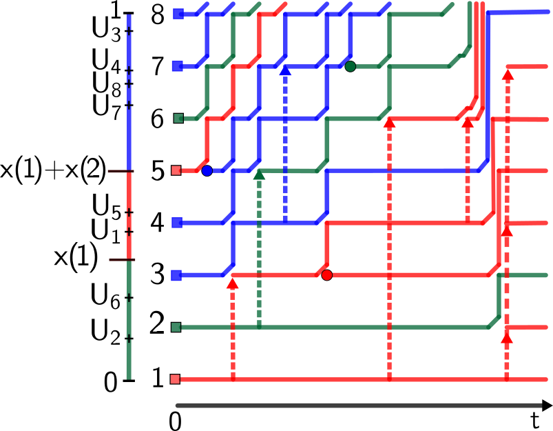
Figure 1. Green, red, and blue lines represent type $1$, type $2$, and type $3$, respectively. The dots represent the mutations.

Formally, let $({\bf{U}}(k))_{k\in\mathbb{N}}$ be a sequence of independent and identically distributed random variables on $[0,1]$ defined on the same probabilistic setup as the Poisson random measures (but independent from them). Fix ${\bf{x}}\in\Delta_{d}$. For each level $k\in\mathbb{N}$, we construct a piecewise constant function $\ell^{{\bf{x}}}_{\cdot}(k):\mathbb{R}_{+}\to[0,1]\times\Delta_{d}$ that codes the individual on level $k$ at time $t$ under initial type assignment ${\bf{x}}$. Set $\ell_{{0}}^{{{\bf{x}}}}\left({k}\right)=({\bf{U}}(k),{\bf{x}})$; that is, initially each individual is characterised by a number in $[0,1]$ and a probability vector of the initial distribution of types. Then an individual’s type can be evaluated via $\mathsf{t}(u,{\bf{x}})$ of (5). The dynamics on the first level is such that $\ell^{{\bf{x}}}(1)\coloneqq(\ell^{{\bf{x}}}_{t}(1))_{t\geq 0}$ only changes upon mutations, that is, if $(t,u)\in\mathcal{M}_{1}$, then set $\ell_{t}^{{\bf{x}}}(1)=(u,{\boldsymbol{\nu}})$ (otherwise nothing changes). Let $n>1$ and assume $\ell^{{\bf{x}}}(k)\coloneqq(\ell_{{t}}^{{{\bf{x}}}}\left({k}\right))_{t\geq 0}$ has been constructed for all $k\leq n-1$. Given $\{\ell^{{\bf{x}}}(k):\,k\leq n-1\}$, define $\ell_{{t}}^{{{\bf{x}}}}\left({n}\right)$ for $t>0$ as follows. In between points of the Poisson random measures, $\ell^{{\bf{x}}}(n)$ stays constant. At points of the Poisson random measures do the following:

• If $t\in\mathcal{P}_{i,j}$, set

  $$\ell_{{t}}^{{{\bf{x}}}}\left({n}\right)=\begin{cases}\ell_{{t-}}^{{{\bf{x}}}}\left({n}\right),&\text{if }n<j,\\ \ell_{{t-}}^{{{\bf{x}}}}\left({i}\right),&n=j,\\ \ell_{{t-}}^{{{\bf{x}}}}\left({n-1}\right),&n>j.\end{cases}$$

• If $(t,r,{\bf{u}})\in\mathcal{N}$, set

  $$\ell_{{t}}^{{{\bf{x}}}}\left({n}\right)=\begin{cases}\ell_{{t-}}^{{{\bf{x}}}}\left({n}\right),&\text{if }\lvert\{l\leq n:{\bf{u}}(l)\leq r\}\rvert=0,\\ \ell_{{t-}}^{{{\bf{x}}}}\left({n-\lvert\{l\leq n:\,{\bf{u}}(l)\leq r\}\rvert+1}\right),&\text{if }{\bf{u}}(n)>r\text{ and }\lvert\{l\leq n:{\bf{u}}(l)\leq r\}\rvert>0,\\ \ell_{{t-}}^{{{\bf{x}}}}\left({\min\{l:\,{\bf{u}}(l)\leq r\}}\right),&\text{if }{\bf{u}}(n)\leq r.\end{cases}$$

• If $(t,u)\in\mathcal{M}_{i}$, set

  $$\ell_{{t}}^{{{\bf{x}}}}\left({n}\right)=\begin{cases}\ell_{{t-}}^{{{\bf{x}}}}\left({n}\right),&\text{if }n<i,\\ (u,{\boldsymbol{\nu}}),&n=i,\\ \ell_{{t-}}^{{{\bf{x}}}}\left({n-1}\right),&n>i,\end{cases}$$

with ${\boldsymbol{\nu}}$ being the mutation vector. The type of the individual occupying level $n$ at time $t$ then is $\mathsf{t}(\ell_{{t}}^{{{\bf{x}}}}\left({n}\right))$, where ${\bf{x}}$ is the initial type distribution. For each $N\in\mathbb{N}$ and initial type distribution ${\bf{x}}\in\Delta_{d}$, the empirical distribution among the first $N$ levels at time $t\geq 0$ is ${\bf{X}}_{t}^{{\bf{x}},N}\in\Delta_{d}$ defined via

$${\bf{X}}^{{\bf{x}},N}_{t}(i)\coloneqq\frac{1}{N}\sum_{n=1}^{N}{\mathds{1}_{\{\mathsf{t}(\ell_{{t}}^{{{\bf{x}}}}\left({n}\right))=i\}}},\quad i\in[d+1].$$

Write ${\bf{X}}^{{\bf{x}},N}=\left({\bf{X}}_{t}^{{\bf{x}},N}\right)_{t\geq 0}$. Let $\mathcal{D}_{[0,\infty)}(\Delta_{d})$ be the càdlàg-functions with values in $\Delta_{d}$ and equip them with the topology induced by $\rho(f,g)\coloneqq\int_{0}^{\infty}e^{-t}\rVert f(t)-g(t)\lVert_{2}^{2}\,\textnormal{d}t$ for $f,g\in\mathcal{D}_{[0,\infty)}(\Delta_{d})$. The following result holds.

Theorem 1 (Convergence).

For all ${\bf{x}}\in\Delta_{d}$,

$${\bf{X}}^{{\bf{x}},N}\xRightarrow[N\to\infty]{(\rho)}{\bf{X}}^{\bf{x}},$$

where ${\bf{X}}^{\bf{x}}$ is the Markov process with generator $\mathcal{A}$ and ${\bf{X}}_{0}^{\bf{x}}={\bf{x}}$.

Theorem 1 is a special case of Birkner et al. [3, Thm. 1.1] for a finite set of types if $\theta=0$. If $\theta>0$, Birkner et al. [3, Thm. 1.1] does not apply because our mutation mechanism is implemented differently into the lookdown-construction. We provide a proof different from the one given in Birkner et al. [3, Thm. 1.1] in Section 3. Our proof makes use of moment duality.

Note that the processes $\{{\bf{X}}^{{\bf{x}}}:{\bf{x}}\in\Delta_{d}\}$ are constructed on one common probability space. We will estbalish that the construction possesses the following crucial feature: whenever two of these processes have the same value at the some time, their paths coalesce and their values agree from then onwards. To study their coalescence time, the following definition is crucial. It generalises the concept of a fixation line to lookdown models with mutation.

Definition 1 (Fixation line).

The fixation line of level $k\in\mathbb{N}_{0}$ is the process $F^{k}=(F^{k}_{t})_{t\geq 0}$ on $\mathbb{N}_{0}$ defined for $k\geq 1$

$$F_{t}^{k}=\max\left\{n\in\mathbb{N}:\ \forall 0<m\leq n,\ \mathsf{t}(\ell_{{t}}^{{{\bf{x}}}}\left({m}\right))\text{ is measurable w.r.t. }\mathscr{F}_{t}\vee\sigma({\bf{U}}(j):1\leq j\leq k)\right\},$$

with the convention that $\max\emptyset=0$ and

$$F_{t}^{0}=\max\left\{n\in\mathbb{N}:\ \forall 0<m\leq n,\ \mathsf{t}(\ell_{{t}}^{{{\bf{x}}}}\left({m}\right))\text{ is measurable w.r.t. }\mathscr{F}_{t}\right\}.$$

In Layman’s terms: $F_{t}^{k}$ is the level at time $t$, such that the type on all levels $m\leq F_{t}^{k}$ at time $t$ can be determined by the information of the Poisson random measures (up to time $t$) and the outcome of ${\bf{U}}(1),\ldots,{\bf{U}}(k)$. When there are no mutations, then $F_{t}^{0}\equiv 0$ for all $t\geq 0$. See also Figure 2 for an illustration of the fixation lines embedded in Figure 1.

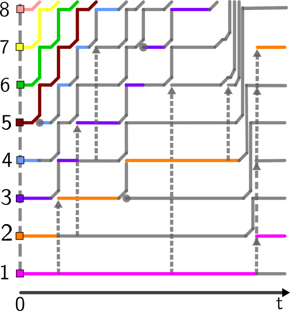
Figure 2. Each color corresponds to a different fixation line in the lookdown-construction of Figure 1.

Remark 1.

In the context of $\theta=0$, Hénard [14, Sect. 2.1] defined the $k$-th fixation line at time $t$ as the smallest level $\ell$ such that level $\ell+1$ carries (at time $t$) an offspring of the individual occupying level $k+1$ at time $0$. When $\theta=0$, his notion and ours are equivalent. See also Hénard [14, Sect. 1] for an overview of the notion of fixation line (this includes a discussion of [21] and [16, 15]).

The next proposition essentially follows from Hénard [14, Lem. 2.3], its proof is in Section 4.

Proposition 1 (Fixation line rates).

For each $k\in\mathbb{N}_{0}$, $F^{k}$ is a continuous-time Markov chain with $F^{k}_{0}=k$ that jumps from $n$ to $n+l$ at rate

$${\mathds{1}_{\{l=1\}}}\bigg{[}\Lambda(\{0\})\binom{n+1}{2}+\theta(n+1)\bigg{]}+\binom{n+l}{l+1}\int_{(0,1]}r^{l+1}(1-r)^{n}\frac{\Lambda(\textnormal{d}r)}{r^{2}},\qquad l\geq 1.$$

Observe that $\left\{F^{k}=(F^{k}_{t})_{t\geq 0}:\,k\in\mathbb{N}\right\}$ are also coupled on a common probability space.

Definition 2 (Explosion time).

For each $k,n\in\mathbb{N}_{0}$ with $n\geq k$, the generalized right inverse of $F^{k}$ is defined as $I^{k}(n)\coloneqq\inf\{t\geq 0:F_{t}^{k}\geq n\}$. Moreover, the explosion time of $F^{k}$ is

$$I^{k}(\infty)\coloneqq\inf\{t\geq 0:\,F_{t}^{k}=\infty\},$$

where $\inf\emptyset=\infty$.

From now on, we impose conditions so that for every $k\in\mathbb{N}$, $I^{k}(\infty)<\infty$ a.s.. This is equivalent to

(6) the associated $$\Lambda$$-coalescent comes down from infinity.

See for example, Herriger and Möhle [13, Thm. 2.4] or Schweinsberg [23] for verifiable conditions which ensure that the associated $\Lambda$-coalescent comes down from infinity.

Example 1 (Coming down from infinity).

  

1. If there is a Kingman-component, i.e. $\Lambda(\{0\})>0$, then, the associated $\Lambda$-coalescent comes down from infinity, see e.g. Berestycki [2, Thm. 2.1].

2. If $\Lambda$ has $\mathrm{Beta}\ (2-\alpha,\alpha)$-distribution with $\alpha\in(1,2)$. i.e. is given by (1), then the associated coalescent comes down from infinity, see e.g. Berestycki [2, Cor. 3.2].

For every $j\in\mathbb{N}$, denote by $p_{t}^{j}$ the proportion of the population at time $t$ that descend from the individual on level $j$ at time $0$, i.e.

$$p_{t}^{j}\coloneqq\lim_{N\to\infty}\frac{1}{N}\sum_{k=1}^{N}{\mathds{1}_{\{\ell_{{t}}^{{{\bf{x}}}}\left({k}\right)=({\bf{U}}(j),{\bf{x}})\}}},\qquad t\geq 0.$$

Since the random variables $\{{\bf{U}}(i),i\geq\mathbb{N}\}$ are independent and Uniform$[0,1]$, we have $({\bf{U}}(i),{\bf{x}})\neq({\bf{U}}(j),{\bf{x}})$ for all $i\neq j$ almost surely. Condition (6) ensures that for each $j\leq k+1$, the value $p_{t}^{j}$ is strictly positive for $t<I^{k}(\infty)$. The next lemma makes this precise, its proof is in Section 4.

Lemma 1.

If condition (6) holds, then almost surely for all $k\in\mathbb{N}$, we have that $p_{t}^{j}>0$ for all $j\leq k+1$ and $t\in[0,I^{k}(\infty))$. Additionally, $p_{t}^{j}=0$ for all $j\geq k+1$ and $t\geq I^{k}(\infty).$

For two initial type frequency distributions ${\bf{x}},{\bf{y}}\in\Delta_{d}$, there will be a first level for which the types at time $0$ differ. More precisely, let $D_{{\bf{x}},{\bf{y}}}\coloneqq\min\{i:\mathsf{t}({\bf{U}}(i),{\bf{x}})\neq\mathsf{t}({\bf{U}}(i),{\bf{y}})\}$, i.e. the first level under which the initial type assignment under ${\bf{x}}$ and ${\bf{y}}$ disagrees.

Theorem 2 (Coalescence times).

If condition (6) holds, then, almost surely, for all ${\bf{x}},{\bf{y}}\in\Delta_{d}$, the coalescence time of the processes with paths started at ${\bf{x}}$ and ${\bf{y}}$, is given by

$$T_{\mathrm{coal}}^{{\bf{x}},{\bf{y}}}\coloneqq\inf\left\{t\geq 0:{\bf{X}}_{t}^{{\bf{x}}}={\bf{X}}_{t}^{{\bf{y}}}\right\}=I^{D_{{\bf{x}},{\bf{y}}}-1}(\infty).$$

Because the proof idea plays a crucial role in all subsequent results, we provide it here.

Proof of Theorem 2.

The main idea is that the type of the individual occupying level $D_{{\bf{x}},{\bf{y}}}$ at time $0$ differs under ${\bf{x}}$ and ${\bf{y}}$, whereas individuals on the first $D_{{\bf{x}},{\bf{y}}}-1$ levels have the same type under ${\bf{x}}$ and ${\bf{y}}$. Distinguish $t\geq I^{D_{{\bf{x}},{\bf{y}}}-1}(\infty)$ and $t<I^{D_{{\bf{x}},{\bf{y}}}-1}(\infty)$. In the former case, by Lemma 1, $p_{t}^{j}=0$ for all $j\geq D_{{\bf{x}},{\bf{y}}}$ and thus ${\bf{X}}_{t}^{{\bf{x}}}={\bf{X}}_{t}^{{\bf{y}}}$. For the latter case, assume $\mathsf{t}(U_{D_{{\bf{x}},{\bf{y}}}},{\bf{x}})=v$ and $\mathsf{t}(U_{D_{{\bf{x}},{\bf{y}}}},{\bf{y}})=w$ for $v\neq w$. We will show that ${\bf{X}}_{t}^{{\bf{x}}}(1)+\cdots+{\bf{X}}_{t}^{{\bf{x}}}(v)\neq{\bf{X}}_{t}^{{\bf{y}}}(1)+\cdots+{\bf{X}}_{t}^{{\bf{y}}}(v)$, which implies ${\bf{X}}_{t}^{{\bf{x}}}\neq{\bf{X}}_{t}^{{\bf{y}}}$. Without loss of generality, assume $v<w$. We then have $\sum_{i=1}^{v-1}{\bf{x}}(i)\leq U_{D_{{\bf{x}},{\bf{y}}}}<\sum_{i=1}^{v}{\bf{x}}(i)$ and $\sum_{i=1}^{v-1}{\bf{y}}(i)\leq\sum_{i=1}^{v}{\bf{y}}(i)\leq\sum_{i=1}^{w-1}{\bf{y}}(i)\leq U_{D_{{\bf{x}},{\bf{y}}}}<\sum_{i=1}^{v}{\bf{y}}(i)$. In particular, for all $u\in[0,1]$, if $\mathsf{t}(u,{\bf{y}})\leq v$, then also $\mathsf{t}(u,{\bf{x}})\leq v$. Because in our setting the $\Lambda$-coalescent comes down from infinity, $\xi_{t}\coloneqq\max\{k\in\mathbb{N}:p_{t}^{k}>0\}<\infty$ for any $t>0$ a.s. Thus,

$${\bf{X}}_{t}^{{\bf{x}}}(1)+\ldots+{\bf{X}}_{t}^{{\bf{x}}}(v) =\frac{1}{\xi_{t}}\sum_{i=1}^{\xi_{t}}{\mathds{1}_{\{\{\mathsf{t}(U_{i},{\bf{x}})\leq v\}\}}}p_{t}^{i}$$

$$=\frac{1}{\xi_{t}}\sum_{i=1}^{\xi_{t}}{\mathds{1}_{\{\{\mathsf{t}(U_{i},{\bf{x}})\leq v\}\}}}({\mathds{1}_{\{\{\mathsf{t}(U_{i},{\bf{y}})\leq v\}\}}}+{\mathds{1}_{\{\{\mathsf{t}(U_{i},{\bf{y}})>v\}\}}})p_{t}^{i}$$

$$\geq{\bf{X}}_{t}^{{\bf{y}}}(1)+\ldots+{\bf{X}}_{t}^{{\bf{y}}}(v)+\frac{1}{\xi_{t}}p_{t}^{D_{{\bf{x}},{\bf{y}}}}>{\bf{X}}_{t}^{{\bf{y}}}(1)+\ldots+{\bf{X}}_{t}^{{\bf{y}}}(v),$$

where in the last step we used that by Lemma 1, $p_{t}^{j}>0$ for all $j\leq D_{{\bf{x}},{\bf{y}}}$ and $t<I^{D_{{\bf{x}},{\bf{y}}}-1}(\infty)$. This completes the proof. ∎

Remark 2 (A comb-like metric).

Note that the previous result yields a random metric on $\Delta_{d}$. To this end, given ${\bf{U}}=({\bf{U}}(i))_{i\in\mathbb{N}}$ on $[0,1]^{\infty}$, define $d_{{\bf{U}}}({\bf{x}},{\bf{y}})\coloneqq I^{D_{{\bf{x}},{\bf{y}}}-1}(\infty)$ for ${\bf{x}},{\bf{y}}\in\Delta_{d}$. This defines a metric on $\Delta_{d}$ (even an ultrametric, i.e. $d_{{\bf{U}}}({\bf{x}},{\bf{z}})\leq\max\{d_{{\bf{U}}}({\bf{x}},{\bf{z}}),d_{{\bf{U}}}({\bf{z}},{\bf{y}})\})$. In the two types case $d=1$, there seems to be a relation to the comb metric [17, Prop. 3.1]. A comb is a function $f:[0,\infty)\to[0,\infty)$ such that for any $\varepsilon>0$, $\{f\geq\varepsilon\}$ is a finite set. The corresponding comb metric $d_{f}(x,y)\coloneqq\sup_{z\in(x\wedge y,x\vee y)}f(z)$ defines a ultrametric distance on $\{f=0\}$. The function given by $C(x)=\sum_{j\geq 1}I^{j}(\infty){\mathds{1}_{\{{\bf{U}}(i)\}}}(x)$ is a comb (since, because of (6), there are only finitely many $j$ such that $I^{j}(\infty)>\varepsilon$ a.s., see proof of Theorem 2). In particular, for $x,y\in[0,1]$, $d_{C}(x,y)=d_{{\bf{U}}}(x,y)$. Note that if $(I^{j}(\infty))_{j\in\mathbb{N}}$ were independent (which they are not!), $d_{{\bf{U}}}(x,y)$ would be the Kingman comb defined in Lambert and Schertzer [17, Prop. 3.1].

Theorem 2 has a couple of useful consequences for deducing explicit, computable expressions for fixation and stationary times.

2.1. Fixation times

Throughout this subsection, we assume $\theta=0$, i.e. there are no mutations. We start out with presenting the consequences of Theorem 2 for fixation times. The following corollary is an immediate consequence of the theorem and we therefore state it without proof.

Corollary 1 (Fixation time).

Assume $\theta=0$. If condition (6) holds, then almost surely, for all ${\bf{x}}\in\Delta_{d}$,

$$\inf\{t\geq 0:\,{\bf{X}}_{t}^{{\bf{x}}}={\bf{e}}_{{k}}\}=\begin{cases}I^{D_{{\bf{x}},{\bf{e}}_{{k}}}-1}(\infty),&\text{if}\ \ \mathsf{t}({\bf{U}}(1),{\bf{x}})=k,\\ \infty,&\text{else.}\end{cases}$$

As a first example where the construction can be exploited is concerned with the probability for types to disappear in a given sequence. To this end, define for $k\in[d+1]$,

$$T_{\mathrm{lost},k}^{{\bf{x}}}\coloneqq\inf\{t\geq 0:{\bf{X}}_{t}^{{\bf{x}}}(k)=0\}\quad\text{and}\quad T_{\mathrm{fix},k}^{{\bf{x}}}\coloneqq\min_{\begin{subarray}{c}J\subset[d+1]\\ k+\lvert J|=d+1\end{subarray}}\max_{j\in J}T_{\mathrm{lost},j}^{{\bf{x}}},$$

i.e. the time where type $k$ disappears from the population and the first time that there are only $k$ types in the population, respectively. Let us recall from Gonzalez Casanova and Smadi [12, Prop. 3.4] that alleles are lost successively and so $T_{\mathrm{fix},k}^{{\bf{x}}}$ is indeed well-defined.

Proposition 2 (Order of disappearance).

Assume $\theta=0$ and condition (6) holds. Fix $i_{1},\ldots,i_{d+1}\in[d+1]$ all distinct. Then,

$$\mathbb{P}(T_{\mathrm{lost},{i_{d+1}}}^{{\bf{x}}}<\cdots<T_{\mathrm{lost},{i_{1}}}^{{\bf{x}}})=\prod_{k=1}^{d+1}\frac{{\bf{x}}(i_{k})}{\sum_{l=k}^{d+1}{\bf{x}}(i_{l})}.$$

The previous proposition implies that the probability for a given disappearance sequence depends only on the initial frequencies, and it is independent of the measure $\Lambda$. Proposition 2 is proved in Section 6.1. The following corollary follows immediately from the preceding proposition and is therefore stated without proof.

Corollary 2 (First type to disappear).

Assume $\theta=0$ and condition (6) holds. For $\eta\in[d+1]$,

$$\mathbb{P}\Big{(}\mathrm{argmin}_{k\in[d+1]}\{T_{\mathrm{lost},k}^{{\bf{x}}}\}=\eta\Big{)}=\sum_{\begin{subarray}{c}1\leq i_{1},\ldots,i_{d}\leq d+1\\ \forall\,k\in[d]:\,i_{k}\neq\eta\\ i_{j}\neq i_{l}\end{subarray}}\,\prod_{k=1}^{d}\frac{{\bf{x}}(i_{k})}{1-\sum_{l=1}^{k-1}{\bf{x}}(i_{l})}$$

This is again independent of $\Lambda$ and just depends on the initial frequencies. For example, if $d=3$, the probability that first type $3$ disappears from the population is ${\bf{x}}(1){\bf{x}}(2)((1-{\bf{x}}(1))^{-1}+(1-{\bf{x}}(2))^{-1})$, which is a well-known result if $\Lambda=\delta_{0}$ (see e.g. [8, Thm. 8.1]).

For $k\in[d+1]$, define the first level at time $0$ that is occupied by type-$k$ as

(7) $$\mathfrak{m}^{{\bf{x}}}_{k}\coloneqq\min\{i:\mathsf{t}({\bf{U}}(i),{\bf{x}})=k\}.$$

The first time at which there are only $k$ types in the population is closely related to the explosion time of the fixation line. Define for $k\in[d+1]$ and ${\bf{x}}\in\Delta_{d}$,

$$V_{k}^{{\bf{x}}}=\min\left\{p:\exists J\subseteq[d+1]\text{ with }\lvert J\rvert=k\text{ s.t. }\forall j\in J:\,\mathfrak{m}^{{\bf{x}}}_{j}<p,\,\min_{i\in[d+1]\setminus J}\mathfrak{m}^{{\bf{x}}}_{i}=p\right\},$$

the first level at time $0$ such that below this level there are exactly $k$ types and on that level there is a type that does not belong to these $k$ types. Equivalently, $V_{k}^{{\bf{x}}}$ is the first level at time $0$ such that a $(k+1)$th type appears for the first time. The following Proposition is proved in Section 6.1.

Theorem 3 (Correspondence between fixation and explosion time).

Assume $\theta=0$ and condition (6) holds. Let $k\in[d+1]$ and ${\bf{x}}\in\Delta_{d}$. Then, almost surely,

$$T_{\mathrm{fix},k}^{{\bf{x}}}=I^{V_{k}^{{\bf{x}}}-1}(\infty).$$

Explicit expressions for the explosion time of the fixation line are known for some important cases like the Wright-Fisher diffusion or $\mathrm{Beta}$-coalescents. Moreover, the distribution of $V_{k}^{{\bf{x}}}$ can be derived by comparison with a coupon collector problem with non-uniform collection probabilities. This allows us to obtain explicit expressions for the mean fixation time.

Theorem 4 (First time exactly $k$ types are alive).

  

1. Wright-Fisher diffusion. Assume $\theta=0$ and $\Lambda=\Lambda(\{0\})\delta_{0}$. Then

   $$\mathbb{E}\left[T_{\mathrm{fix},k}^{{\bf{x}}}\right]=-\frac{2}{\Lambda(\{0\})}\sum_{\ell=1}^{k}(-1)^{k-\ell}\binom{d-\ell}{k-\ell}\sum_{1\leq i_{1}<\cdots<i_{\ell}\leq d+1}\left(1-\sum_{j=1}^{\ell}{\bf{x}}(i_{j})\right)\log\left(1-\sum_{j=1}^{\ell}{\bf{x}}(i_{j})\right).$$

2. Beta-coalescent. Assume $\theta=0$ and $\Lambda$ is as in (1) with $\alpha\in(1,2)$. Then

   $$\begin{split}\mathbb{E}\left[T_{\mathrm{fix},k}^{{\bf{x}}}\right]=&\alpha(\alpha-1)\sum_{\ell=1}^{k}(-1)^{k-\ell}\left\{\binom{d-\ell}{k-\ell}\sum_{1\leq i_{1}<\cdots<i_{\ell}\leq d+1}\left(1-\sum_{j=1}^{\ell}{\bf{x}}(i_{j})\right)\left(\sum_{j=1}^{\ell}{\bf{x}}(i_{j})\right)\right.\\ &\cdot\left.\int_{(0,1)}\frac{y(1-y)^{-1}}{\left(1-y\sum_{j=1}^{\ell}{\bf{x}}(i_{j})\right)\left((1-y)^{1-\alpha}-1\right)}\textnormal{d}y\right\}.\end{split}$$

In particular, we recover the well-known mean fixation time formula of the Wright–Fisher diffusion, i.e. for $\Lambda=\delta_{0}$ and $k=1$,

(8) $$\mathbb{E}\left[T_{\mathrm{fix},1}^{{\bf{x}}}\right]=-2\sum_{k=1}^{d+1}\left(1-{\bf{x}}(k)\right)\log\Big{(}1-{\bf{x}}(k)\Big{)}.$$

Littler [19] (see also [8, Ch. 8.1.1]) derived (8) by methods from diffusion theory. Our proof uses elementary probabilistic arguments and it is in Section 6.1. Figure 3 illustrates Theorem 4 by plotting the mean fixation times in the case $d=2$ and $k=1$ for different choices of $\Lambda$.

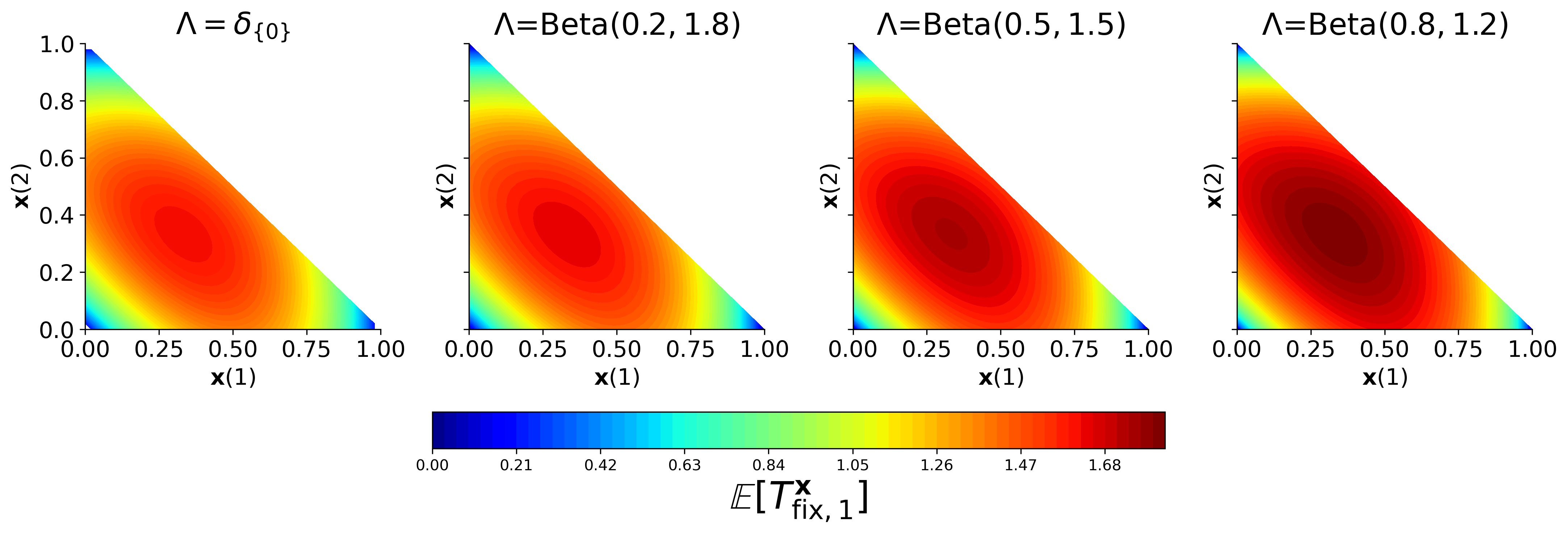
Figure 3. Mean fixation time for $3$ types with initial value ${\bf{x}}(1)$, ${\bf{x}}(2)$, and ${\bf{x}}(3)=1-{\bf{x}}(2)-{\bf{x}}(3)$. From left to right, $\Lambda$ is $\delta_{0}$ and $\mathrm{Beta}(2-\alpha,\alpha)$ for $\alpha=1.8$, $\alpha=1.5$, and $\alpha=1.2$. The darker the colour at ${\bf{x}}$, the larger the mean fixation time when the system is initialised at ${\bf{x}}$. As the parameter $\alpha$ increases, the mean fixation time increases for any ${\bf{x}}\in\Delta_{d}$.

Proposition 3.

Assume $\theta=0$ and $\Lambda=\delta_{0}$. For any $t\in\mathbb{R}$ and $k\in[d+1]$,

$$\mathbb{E}\left[e^{itT_{\mathrm{fix},k}^{{\bf{x}}}}\right]=\sum_{\ell=1}^{k}(-1)^{k-\ell}\binom{d-\ell}{k-\ell}\sum_{1\leq i_{1}<\ldots<i_{\ell}\leq d+1}\Bigg{(}1-{\sum_{j=1}^{\ell}}{\bf{x}}(i_{j})\Bigg{)}\sum_{p=1}^{\infty}\Bigg{(}\sum_{j=1}^{\ell}{\bf{x}}(i_{j})\Bigg{)}^{p}\prod_{r=p}^{\infty}\Big{(}1-\frac{2it}{(r+1)r}\Big{)}^{-1}.$$

The proof of Proposition 3 is in Section 6.1.

2.2. Stationary times

Assume $\theta>0$ and ${\boldsymbol{\nu}}$ is in the interior of $\Delta_{d}$. Here, the notion of a strong stationary time will be useful. This special stopping time was introduced by [5] for Markov chains and has been proven to be a useful tool in the study of stationary times. The tail distribution of the smallest among these times is the separation distance of the chain to the stationary distribution. Recently, there has been increased interest in extending this tool to more general Markov processes [10, 20]. The following definition is adapted from [20]. Consider an ergodic Markov process $X=(X_{t})_{t\geq 0}$ constructed on some probability space $(\Omega,\mathcal{G},P,(\mathcal{G}_{t})_{t\geq 0})$ with invariant distribution $\pi$. A $\mathcal{G}$-stopping time $T$ taking values in $[0,\infty)$ is said to be strong (for $X$) if $T$ and $X_{T}$ are independent. It is said to be a strong stationary time (for $X$) if furthermore $X_{T}$ is distributed according to $\pi$.

Theorem 5 ((Strong) stationary time).

Assume $\theta>0$ and condition (6) holds. $I^{0}(\infty)$ is a stationary time for ${\bf{X}}^{\bf{x}}$ for all ${\bf{x}}\in\Delta_{d}$. Moreover, if $\Lambda=\Lambda(\{0\})\delta_{0}$, then $I^{0}(\infty)$ is a strong stationary time.

The proof of Theorem 5 can be found in Section 6.2. The following corollary is a straightforward consequence of Theorem 5 and the form of the transition rates of the fixation line stated in Proposition 1. Its proof is in Section 6.2.

Corollary 3 (Mean strong stationary time for Wright–Fisher diffusion).

Assume $\theta>0$ and $\Lambda=\Lambda(\{0\})\delta_{0}$. Then the strong stationary time $I^{0}(\infty)$ has the same distribution as $\sum_{j=0}^{\infty}E_{j}$, where $(E_{j})_{j\in\mathbb{N}}$ are independent exponential random variables with $E_{j}$ having parameter $\left(\Lambda(\{0\})\binom{j+1}{2}+(j+1)\theta\right)$. In particular,

$$\mathbb{E}\left[I^{0}(\infty)\right]=\sum_{j=0}^{\infty}\frac{1}{j+1}\frac{1}{\theta+\Lambda(\{0\})j/2}=\frac{\psi\left(2\theta/\Lambda(\{0\})\right)+\gamma}{\theta-\Lambda(\{0\})/2},$$

where $\psi$ is the so-called digamma function and $\gamma$ is the Euler-Mascheroni constant.

3. Convergence of $N$-lookdown type-frequency process to $\Lambda$-Wright–Fisher process

Recall that we equip $\mathcal{D}_{[0,\infty)}(\Delta_{d})$ with the topology induced by $\rho(f,g)=\int_{0}^{\infty}e^{-t}\rVert f(t)-g(t)\lVert_{2}^{2}\,\textnormal{d}t$ for $f,g\in\mathcal{D}_{[0,\infty)}(\Delta_{d})$. The main work of this subsection will be to prove the following lemma.

Lemma 2.

For all ${\bf{x}}\in\Delta_{d}$ and $t\geq 0$, $\mathbb{E}\left[\lVert{\bf{X}}_{t}^{{\bf{x}},N}-{\bf{X}}_{t}^{{\bf{x}}}\rVert_{2}^{2}\right]\xrightarrow{N\to\infty}0$.

We postpone the proof of the lemma and use it now to prove the convergence result.

Proof of Theorem 1.

Fix ${\bf{x}}\in\Delta_{d}$ and $\varepsilon>0$. Then using Markov inequality, Fubini, Lemma 2 and the Dominated Convergence Theorem with the integrable function $2e^{-t}$, we obtain

$$\mathbb{P}\left(\rho({\bf{X}}^{{\bf{x}},N},{\bf{X}}^{{\bf{x}}})>\varepsilon\right)\leq\frac{1}{\varepsilon}\mathbb{E}\left[\rho({\bf{X}}^{{\bf{x}},N},{\bf{X}}^{{\bf{x}}})\right]=\frac{1}{\varepsilon}\int_{0}^{\infty}e^{-t}\mathbb{E}\left[\lVert{\bf{X}}_{t}^{{\bf{x}},N}-{\bf{X}}_{t}^{{\bf{x}}}\rVert_{2}^{2}\right]\textnormal{d}t\xrightarrow{N\to\infty}0.$$

∎

It remains to prove Lemma 2. To this end, we will employ duality. We identify the moment dual of the process described by (2)–(4); and we use it to characterise $\lim_{N\to\infty}{\bf{X}}^{{\bf{x}},N}$. To formally introduce the dual process, we start with its state space $\mathbb{N}_{0,\dagger}^{d}\coloneqq\mathbb{N}_{0}^{d}\cup{\dagger}$, where $\dagger$ is a cemetery state. Define the function $H:\Delta_{d}\times\mathbb{N}_{0,\dagger}^{d}\to[0,1]$ as

(9) $$H({\bf{x}},{\bf{n}})={\bf{x}}^{{\bf{n}}}:=\prod_{k=1}^{d}{\bf{x}}(k)^{{\bf{n}}(k)},\qquad\qquad\mbox{for }{\bf{x}}\in\Delta_{d}\mbox{ and }{\bf{n}}\neq\dagger,$$

and $H({\bf{x}},\dagger)={\bf{x}}^{\dagger}\coloneqq 0$. To start out, we prove the following lemma.

Lemma 3.

For all ${\bf{x}}\in\Delta_{d}$, ${\bf{n}}\in\mathbb{N}_{0,\dagger}^{d}$ and $t\geq 0$,

(10) $$\mathbb{E}[({\bf{X}}_{t}^{{\bf{x}},N})^{{\bf{n}}}]\xrightarrow{N\to\infty}\mathbb{P}\bigg{(}\bigcap_{\begin{subarray}{c}k\in[d]\\ {\bf{n}}(k)>0\end{subarray}}^{d}\Big{\{}\mathsf{t}\left(\ell_{{t}}^{{{\bf{x}}}}\left({1+\sum_{r=1}^{k-1}{\bf{n}}(r)}\right)\right)=\cdots=\mathsf{t}\left(\ell_{{t}}^{{{\bf{x}}}}\left({\sum_{r=1}^{k}{\bf{n}}(r)}\right)\right)=k\Big{\}}\bigg{)}.$$

Proof.

Fix ${\bf{x}}\in\Delta_{d}$, ${\bf{n}}\in\mathbb{N}_{0}^{d}$, $N\geq\lvert{\bf{n}}\rvert$ and $t\geq 0$. Using the definition of ${\bf{X}}_{t}^{{\bf{x}},N}$ and the multinomial theorem,

$$\mathbb{E}\left[\prod_{k=1}^{d}({\bf{X}}_{t}^{{\bf{x}},N}(k))^{{\bf{n}}(k)}\right]$$

$$=\frac{1}{N^{\lvert{\bf{n}}\rvert}}\mathbb{E}\Bigg{[}\prod_{k=1}^{d}\sum_{\begin{subarray}{c}i_{1}^{k}+\cdots+i_{N}^{k}={\bf{n}}(k)\\ i_{1}^{k},\ldots,i_{N}^{k}\geq 0\end{subarray}}\binom{{\bf{n}}(k)}{i_{1}^{k},\ldots,i_{N}^{k}}\prod_{j=1}^{N}{\mathds{1}_{\{\mathsf{t}(\ell_{{t}}^{{{\bf{x}}}}\left({j}\right))=k\}}}^{i_{j}^{k}}\Bigg{]}$$

(11) $$=\frac{1}{N^{\lvert{\bf{n}}\rvert}}\sum_{\ell=0}^{\lvert{\bf{n}}\rvert}\mathbb{E}\bigg{[}\prod_{k=1}^{d}\sum_{\begin{subarray}{c}i_{1}^{k}+\cdots+i_{N}^{k}={\bf{n}}(k)\\ i_{1}^{k},\ldots,i_{N}^{k}\geq 0\end{subarray}}{\mathds{1}_{\{\lvert\{(j,k):i^{k}_{j}\geq 2\}\rvert=\ell\}}}\binom{{\bf{n}}(k)}{i_{1}^{k},\ldots,i_{N}^{k}}\prod_{j=1}^{N}{\mathds{1}_{\{\mathsf{t}(\ell_{{t}}^{{{\bf{x}}}}\left({j}\right))=k\}}}^{i_{j}^{k}}\bigg{]},$$

where $\binom{{\bf{n}}(k)}{i_{1}^{k},\ldots,i_{N}^{k}}={\bf{n}}(k)!/(i_{1}^{k}!\cdots i_{N}^{k}!)$. Now, the general idea is to show that the terms with $\ell\geq 1$ vanish as $N\to\infty$, and the term for $\ell=0$ converges to the probability on the right-hand side of (10). Fist, consider the term associated to $\ell=0$ and note that in this case $i_{j}^{k}\in\{0,1\}$ so that the term reduces to

(12) $$\frac{1}{N^{\lvert{\bf{n}}\rvert}}\mathbb{E}\bigg{[}\prod_{k=1}^{d}\sum_{\begin{subarray}{c}i_{1}^{k}+\cdots+i_{N}^{k}={\bf{n}}(k)\\ i_{1}^{k},\ldots,i_{N}^{k}\in\{0,1\}\end{subarray}}{\bf{n}}(k)!\prod_{j=1}^{N}{\mathds{1}_{\{\mathsf{t}(\ell_{{t}}^{{{\bf{x}}}}\left({j}\right))=k\}}}^{i_{j}^{k}}\bigg{]}$$

For a positive contribution it is necessary that if $i_{j}^{k}=1$, then $i_{j}^{l}=0$ for $l\neq k$. Since $\lvert\{i_{j}^{k}:i_{j}^{k}=1\}\rvert=\lvert{\bf{n}}\rvert$, we first select from $N$ lines $\lvert{\bf{n}}\rvert$ distinct lines. Next, we partition the $\lvert{\bf{n}}\rvert$ lines into ${\bf{n}}(k)$ lines of type $k$ for each $k$. Write $p_{l}^{k}$ for the level of the $l$th line of type $k$, $l\in{\bf{n}}(k)$, $k\in[d]$. Thus, using also exchangeability, we rewrite (12) as

$$\frac{{\bf{n}}(1)!\cdots{\bf{n}}(d)!}{N^{\lvert{\bf{n}}\rvert}}\mathbb{E}\bigg{[}\sum_{\begin{subarray}{c}p_{1}^{k},\ldots,p_{{\bf{n}}(k)}^{k}\in[N]\\ k\in[d],p_{l}^{k}\text{ all distinct}\end{subarray}}\prod_{r=1}^{d}\Big{(}{\mathds{1}_{\{\mathsf{t}(\ell_{{t}}^{{{\bf{x}}}}\left({p_{1}^{r}}\right))=r\}}}\cdots{\mathds{1}_{\{\mathsf{t}(\ell_{{t}}^{{{\bf{x}}}}\left({p_{{\bf{n}}(r)}^{r}}\right))=r\}}}\Big{)}\bigg{]}$$

$$=\frac{{\bf{n}}(1)!\cdots{\bf{n}}(d)!}{N^{\lvert{\bf{n}}\rvert}}\binom{N}{\lvert{\bf{n}}\rvert}\binom{\lvert{\bf{n}}\rvert}{{\bf{n}}(1),\ldots,{\bf{n}}(d)}\mathbb{P}\bigg{(}\bigcap_{\begin{subarray}{c}k\in[d]\\ {\bf{n}}(k)>0\end{subarray}}\Big{\{}\mathsf{t}\left(\ell_{{t}}^{{{\bf{x}}}}\left({p_{1}^{k}}\right)\right)=\cdots=\mathsf{t}\left(\ell_{{t}}^{{{\bf{x}}}}\left({p_{{\bf{n}}(k)}^{k}}\right)\right)=k\Big{\}}\bigg{)}$$

$$=\frac{N\cdots(N-\lvert{\bf{n}}\rvert+1)}{N^{\lvert{\bf{n}}\rvert}}\mathbb{P}\bigg{(}\bigcap_{\begin{subarray}{c}k\in[d]\\ {\bf{n}}(k)>0\end{subarray}}\Big{\{}\mathsf{t}\left(\ell_{{t}}^{{{\bf{x}}}}\left({1+\sum_{r=1}^{k-1}{\bf{n}}(r)}\right)\right)=\cdots=\mathsf{t}\left(\ell_{{t}}^{{{\bf{x}}}}\left({\sum_{r=1}^{k}{\bf{n}}(r)}\right)\right)=k\Big{\}}\bigg{)},$$

which converges to the right-hand side of (10) as $N\to\infty$.

Next, we show that the terms in (11) corresponding to $\ell>0$ vanish as $N\to\infty$. To this end, fix some $\ell\geq 1$ and consider the corresponding summand in (11). Also here, for a positive contribution it is necessary that if $i_{j}^{k}>0$, then $i_{j}^{l}=0$ for $l\neq k$. In particular, we first need to select among $N$ lines $\lvert{\bf{n}}\rvert$ lines, with each line $j$ having $i_{j}^{k}\geq 1$ for some $k$. But in contrast to $\ell=0$, some lines can be chosen twice and so the number of distinct lines is $\lvert{\bf{n}}^{\star}|<\lvert{\bf{n}}\rvert$ for some ${\bf{n}}^{\star}\in\mathbb{N}_{0}^{d}$. In particular, a term with positive contribution has now ${\bf{n}}^{\star}(k)$ lines of type $k$ where ${\bf{n}}^{\star}(k)\leq{\bf{n}}(k)$ and the inequality is strict for at least one $k$. Thus, we can upper bound the term in (11) corresponding to $\ell$ by

$$\frac{{\bf{n}}(1)!\cdots{\bf{n}}(d)!}{N^{\lvert{\bf{n}}\rvert}}\mathbb{E}\bigg{[}\sum_{\begin{subarray}{c}p_{1}^{k}+\cdots+p_{{\bf{n}}^{\star}(k)}^{k}\in[N]\\ k\in[d],p_{l}^{k}\text{ all distinct}\end{subarray}}\prod_{r=1}^{d}\Big{(}{\mathds{1}_{\{\mathsf{t}(\ell_{{t}}^{{{\bf{x}}}}\left({p_{1}^{r}}\right))=r\}}}\cdots{\mathds{1}_{\{\mathsf{t}(\ell_{{t}}^{{{\bf{x}}}}\left({p_{{\bf{n}}^{\star}(r)}^{r}}\right))=r\}}}\Big{)}\bigg{]}$$

$$\leq\frac{{\bf{n}}(1)!\cdots{\bf{n}}(d)!}{N^{\lvert{\bf{n}}\rvert}}\binom{N}{\lvert{\bf{n}}^{\star}\rvert}\binom{\lvert{\bf{n}}^{\star}\rvert}{{\bf{n}}^{\star}(1),\ldots,{\bf{n}}^{\star}(d)}\leq\frac{N-\lvert{\bf{n}}^{\star}\rvert+1}{N^{\lvert{\bf{n}}\rvert}},$$

which converges to $0$ because $\lvert{\bf{n}}^{\star}\rvert<\lvert{\bf{n}}\rvert$. This completes the proof.

∎

To motivate the dual process, we are going to work in the lookdown-construction. Fix ${\bf{x}}\in\Delta_{d}$, ${\bf{n}}\in\mathbb{N}_{0}^{d}$ and $t\geq 0$. Let ${\bf{A}}_{0}^{({\bf{n}})}(i)={\bf{n}}(i)$ and if ${\bf{n}}(i)>0$, call the lines that occupy at time $t$ level $1+\sum_{j=1}^{i-1}{\bf{n}}(j)$ up to level $\sum_{j=1}^{i}{\bf{n}}(j)$ the ancestral lines of type $i$ at time $t$ (if ${\bf{n}}(i)=0$ there are no ancestral lines of type $i$ at time $t$). For $r\in[0,t]$, set ${\bf{A}}_{r}^{({\bf{n}})}(i)$ to be the number of ancestral lines at time $t-r$ of the lines of type $i$ at time $t$. The corresponding lines will be called ancestral lines of type $i$ (at time $t-r$). If at time $t-r$, ancestral lines of type $i$ and $j$ for $i\neq j$ coalesce, we set ${\bf{A}}^{({\bf{n}})}_{s}$ to $\dagger$ for all $s>r$. Similarly, if one of the ancestral lines of type $i$ originates from $\mathcal{M}_{j}$, $j\neq i$, send ${\bf{A}}_{s}^{({\bf{n}})}$ to $\dagger$ for all $s>r$. But if one of the ancestral lines of type $i$ originates from $\mathcal{M}_{i}$, remove the ancestral line (the number of ancestral lines of type $i$ is reduced by one).

Define

$$\lambda_{n,k}\coloneqq\int_{(0,1]}r^{k-2}(1-r)^{n-k}\Lambda(\textnormal{d}r),\qquad 2\leq k\leq n.$$

Motivated by the above discussion, let now ${\bf{A}}^{({\bf{n}})}=({\bf{A}}_{r}^{({\bf{n}})})_{r\geq 0}$ be the process started at ${\bf{n}}$ and with infinitesimal generator $\mathcal{L}=\mathcal{L}_{\mathrm{WF}}+\mathcal{L}_{\Lambda}+\mathcal{L}_{\theta}$ that acts on $g\in\mathcal{B}(\mathbb{N}_{0,\dagger}^{d})$ via

$$\mathcal{L}_{\mathrm{WF}}g({\bf{n}}) =\Lambda(\{0\})\sum_{i=1}^{d}\left({\bf{n}}(i)({\bf{n}}(i)-1)[g({\bf{n}}-{\bf{e}}_{{i}})-g({\bf{n}})]+\sum_{\begin{subarray}{c}j=1\\ j\neq i\end{subarray}}^{d}{\bf{n}}(i){\bf{n}}(j)[g(\dagger)-g({\bf{n}})]\right),$$

$$\mathcal{L}_{\Lambda}g({\bf{n}}) =\sum_{i=1}^{d}\sum_{k=2}^{{\bf{n}}(i)}\binom{{\bf{n}}(i)}{k}\lambda_{\lvert{\bf{n}}\rvert,k}[g({\bf{n}}-(k-1){\bf{e}}_{{i}})-g({\bf{n}})]$$

$$\quad+\int_{(0,1]}\left(1-(1-r)^{\lvert{\bf{n}}\rvert}-\sum_{i=1}^{d}\sum_{k=1}^{{\bf{n}}(i)}\binom{{\bf{n}}(i)}{k}(1-r)^{\lvert{\bf{n}}\rvert-k}r^{k}\right)\frac{\Lambda(\textnormal{d}r)}{r^{2}}[g(\dagger)-g({\bf{n}})],$$

$$\mathcal{L}_{\theta}g({\bf{n}}) =\theta\sum_{i=1}^{d}{\bf{n}}(i)\left({\boldsymbol{\nu}}(i)[g({\bf{n}}-{\bf{e}}_{{i}})-g({\bf{n}})]+\sum_{\begin{subarray}{c}j=1\\ j\neq i\end{subarray}}^{d}{\boldsymbol{\nu}}(j)[g(\dagger)-g({\bf{n}})]\right).$$

with $\mathcal{L}_{\mathrm{WF}}g(\dagger)=\mathcal{L}_{\Lambda}g(\dagger)=\mathcal{L}_{\theta}g(\dagger)=0$.

Remark 3.

Note that for $\mathcal{L}_{\Lambda}$, the rate at which a transition to $\dagger$ occurs can be rewritten as

$$\int_{(0,1]}\Big{(}1-(1-r)^{\lvert{\bf{n}}\rvert}-\lvert{\bf{n}}\rvert(1-r)^{\lvert{\bf{n}}\rvert-1}r-\sum_{i=1}^{d}\sum_{k=2}^{{\bf{n}}(i)}\binom{{\bf{n}}(i)}{k}(1-r)^{\lvert{\bf{n}}\rvert-k}r^{k}\Big{)}\frac{\Lambda(\textnormal{d}r)}{r^{2}},$$

which we indeed recognise as the rate at which at least two lines are selected to coalesce and not all the coalescing lines are of the same type.

Recall the definition of $H$ in (9).

Theorem 6 (Moment duality).

Let ${\bf{X}}$ be the process generated by (2)–(4). Then, for all ${\bf{x}}\in\Delta_{d}$ and all ${\bf{n}}\in\mathbb{N}_{0,\dagger}^{d}$, we have

$$\mathbb{E}[H({\bf{X}}_{t}^{{\bf{x}}},{\bf{n}})]=\mathbb{E}[H({\bf{x}},{\bf{A}}_{t}^{({\bf{n}})})].$$

Proof.

Recall the definition of the generator $\mathcal{A}$ of ${\bf{X}}^{{\bf{x}}}$ from (2)–(4). We have to show that

(13) $$\mathcal{A}H({\bf{x}},{\bf{n}})=\mathcal{L}H({\bf{x}},{\bf{n}})\qquad\mbox{for all }{\bf{x}},{\bf{n}}.$$

Since ${\bf{A}}^{({\bf{n}})}$ is a non-explosive Markov chain and ${\bf{X}}^{{\bf{x}}}$ is Feller, the theorem follows from Liggett [18, Thm. 3.42]. (To see the Feller property, recall that the one-dimensional projections are Feller, e.g. [4, Prop. B.5]. Checking the Feller property of ${\bf{X}}^{{\bf{x}}}$ is then a straightforward calculation). To show (13), we match the respective parts of the generators. Clearly,

(14) $$\frac{\partial}{\partial{\bf{x}}(i)}H({\bf{x}},{\bf{n}})={\bf{n}}(i)H({\bf{x}},{\bf{n}}-{\bf{e}}_{{i}})\quad\text{and}\quad\frac{\partial^{2}}{\partial{\bf{x}}(i)\partial{\bf{x}}(j)}H({\bf{x}},{\bf{n}})={\bf{n}}(i)({\bf{n}}(j)-{\mathds{1}_{\{i\}}}(j))H({\bf{x}},{\bf{n}}-{\bf{e}}_{{i}}-{\bf{e}}_{{j}}).$$

Using (14), we see that

$$\mathcal{A}_{\mathrm{WF}}H(\cdot,{\bf{n}})({\bf{x}}) =\Lambda(\{0\})\sum_{i=1}^{d}\Bigg{(}\binom{{\bf{n}}(i)}{2}[H({\bf{x}},{\bf{n}}-{\bf{e}}_{{i}})-H({\bf{x}},{\bf{n}})]-\sum_{\begin{subarray}{c}j=1\\ j\neq i\end{subarray}}^{d}{\bf{n}}(i){\bf{n}}(j)H({\bf{x}},{\bf{n}})\Bigg{)}$$

$$=\mathcal{L}_{\mathrm{WF}}H({\bf{x}},\cdot)({\bf{n}})$$

and

$$\mathcal{A}_{\theta}H(\cdot,{\bf{n}})({\bf{x}}) =\theta\sum_{i=1}^{d}{\bf{n}}(i)\Bigg{(}{\boldsymbol{\nu}}(i)[H({\bf{x}},{\bf{n}}-{\bf{e}}_{{i}})-H({\bf{x}},{\bf{n}})]+\sum_{j\neq i}{\boldsymbol{\nu}}(j)[H({\bf{x}},\dagger)-H({\bf{x}},{\bf{n}})]\Bigg{)}$$

$$=\mathcal{L}_{\theta}H({\bf{x}},\cdot)({\bf{n}}).$$

For the $\Lambda$-part, we also use the definition of $H$, but the computation is slightly more involved:

$$\mathcal{A}_{\Lambda}H(\cdot,{\bf{n}})({\bf{x}})= \int_{(0,1]}\Bigg{(}\sum_{i=1}^{d+1}H((1-r){\bf{x}}+r{\bf{e}}_{{i}},{\bf{n}})\Bigg{)}-H({\bf{x}},{\bf{n}})\frac{\Lambda(\textnormal{d}r)}{r^{2}}$$

$$= \int_{(0,1]}\Bigg{(}\Bigg{\{}\sum_{i=1}^{d}\Bigg{[}\sum_{k=0}^{{\bf{n}}(i)}\binom{{\bf{n}}(i)}{k}r^{k}{\bf{x}}(i)^{{\bf{n}}(i)-k+1}(1-r)^{\lvert{\bf{n}}\rvert-k}\prod_{\begin{subarray}{c}\ell=1\\ \ell\neq i\end{subarray}}^{d}{\bf{x}}(\ell)^{{\bf{n}}(\ell)}\Bigg{]}$$

$$+\bigg{(}1-\sum_{i=1}^{d}{\bf{x}}(i)\bigg{)}(1-r)^{|{\bf{n}}\rvert}{\bf{x}}^{{\bf{n}}}\Bigg{\}}-{\bf{x}}^{{\bf{n}}}\Bigg{)}\frac{\Lambda(\textnormal{d}r)}{r^{2}}$$

$$= \int_{(0,1]}\Bigg{(}\sum_{i=1}^{d}\Bigg{[}\sum_{k=1}^{{\bf{n}}(i)}\binom{{\bf{n}}(i)}{k}r^{k}{\bf{x}}(i)^{{\bf{n}}(i)-k+1}(1-r)^{\lvert{\bf{n}}\rvert-k}\prod_{\begin{subarray}{c}\ell=1\\ \ell\neq i\end{subarray}}^{d}{\bf{x}}(\ell)^{{\bf{n}}(\ell)}\Bigg{]}$$

$$-\Big{(}1-(1-r)^{\lvert{\bf{n}}\rvert}\Big{)}{\bf{x}}^{{\bf{n}}}\Bigg{)}\frac{\Lambda(\textnormal{d}r)}{r^{2}}$$

$$= \int_{(0,1]}\Bigg{(}\sum_{i=1}^{d}\Bigg{[}\sum_{k=2}^{{\bf{n}}(i)}\binom{{\bf{n}}(i)}{k}r^{k}{\bf{x}}(i)^{{\bf{n}}(i)-k+1}(1-r)^{\lvert{\bf{n}}\rvert-k}\prod_{\begin{subarray}{c}\ell=1\\ \ell\neq i\end{subarray}}^{d}{\bf{x}}(\ell)^{{\bf{n}}(\ell)}\Bigg{]}$$

$$-\Big{(}1-(1-r)^{\lvert{\bf{n}}\rvert}-\lvert{\bf{n}}\rvert r(1-r)^{\lvert{\bf{n}}\rvert-1}\Big{)}{\bf{x}}^{{\bf{n}}}\Bigg{)}\frac{\Lambda(\textnormal{d}r)}{r^{2}}$$

$$= \sum_{i=1}^{d}\sum_{k=2}^{{\bf{n}}(i)}\binom{{\bf{n}}(i)}{k}\lambda_{\lvert{\bf{n}}\rvert,k}\Big{[}H({\bf{x}},{\bf{n}}-(k-1){\bf{e}}_{{i}})-H({\bf{x}},{\bf{n}})\Big{]}+[H({\bf{x}},\dagger)-H({\bf{x}},{\bf{n}})]$$

$$\cdot\int_{(0,1]}\Bigg{(}1-(1-r)^{\lvert{\bf{n}}\rvert}-\lvert{\bf{n}}\rvert r(1-r)^{\lvert{\bf{n}}\rvert-1}-\sum_{i=1}^{d}\sum_{k=2}^{{\bf{n}}(i)}\binom{{\bf{n}}(i)}{k}r^{k}(1-r)^{\lvert{\bf{n}}\rvert-k}\Bigg{)}\frac{\Lambda(\textnormal{d}r)}{r^{2}}$$

$$= \mathcal{L}_{\Lambda}H({\bf{x}},\cdot)({\bf{n}}).$$

∎

We will use now the relation between the dual process and the process that tracks ancestral lines in the lookdown construction. Let ${\bf{n}}\in\mathbb{N}_{0}^{d}$ and at time $t$, select the first $\lvert{\bf{n}}\rvert$ lines in the $N$-lookdown (with $N\geq\lvert{\bf{n}}\rvert$). The probability that the first ${\bf{n}}(1)$ lines are of type $1$, the next ${\bf{n}}(2)$ lines are of type $2$, …, and the last ${\bf{n}}(d)$ lines are of type $d$ can be computed by following their ancestral lines backward in time, and then requiring that all ancestors of type-$i$ lines are of type $i$. The next lemma formalises this idea.

Lemma 4.

For all ${\bf{x}}\in\Delta_{d}$, ${\bf{n}}\in\mathbb{N}_{0}^{d}$ and $t\geq 0$,

(15) $$\mathbb{E}\left[{\bf{x}}^{{\bf{A}}_{t}^{({\bf{n}})}}\right]=\mathbb{P}\Big{(}\bigcap_{\begin{subarray}{c}k\in[d]\\ {\bf{n}}(k)>0\end{subarray}}^{d}\Big{\{}\mathsf{t}\left(\ell_{{t}}^{{{\bf{x}}}}\left({1+\sum_{r=1}^{k-1}{\bf{n}}(r)}\right)\right)=\cdots=\mathsf{t}\left(\ell_{{t}}^{{{\bf{x}}}}\left({\sum_{r=1}^{k}{\bf{n}}(r)}\right)\right)=k\Big{\}}\Big{)}.$$

Proof.

Fix ${\bf{x}}\in\Delta_{d}$, ${\bf{n}}\in\mathbb{N}_{0}^{d}$ and $t\geq 0$. From the interpretation of ${\bf{A}}$ in terms of ancestral lines, it can be shown via induction on the number of events in $[0,t]$ that

$$\bigcap_{\begin{subarray}{c}k\in[d]\\ {\bf{n}}(k)>0\end{subarray}}^{d}\Big{\{}\mathsf{t}\left(\ell_{{t}}^{{{\bf{x}}}}\left({1+\sum_{r=1}^{k-1}{\bf{n}}(r)}\right)\right)=\cdots=\mathsf{t}\left(\ell_{{t}}^{{{\bf{x}}}}\left({\sum_{r=1}^{k}{\bf{n}}(r)}\right)\right)=k\Big{\}}$$

is equivalent to

$$\bigcap_{\begin{subarray}{c}k\in[d]\\ {\bf{A}}_{t}(k)>0\end{subarray}}^{d}\Big{\{}\mathsf{t}\left(\ell_{{0}}^{{{\bf{x}}}}\left({1+\sum_{r=1}^{k-1}{\bf{A}}_{t}(r)}\right)\right)=\cdots=\mathsf{t}\left(\ell_{{0}}^{{{\bf{x}}}}\left({\sum_{r=1}^{k}{\bf{A}}_{t}(r)}\right)\right)=k\Big{\}},$$

with the convention that $\dagger+k=\dagger$ for any $k\in\mathbb{N}_{0}$. In particular, (15) follows

∎

Finally, we combine the previous lemmas to obtain that $\lim_{N\to\infty}{\bf{X}}^{{\bf{x}},N}$ has indeed generator $\mathcal{A}$.

Lemma 5.

For all ${\bf{x}}\in\Delta_{d}$ and $t\geq 0$, $\lim_{N\to\infty}{\bf{X}}_{t}^{{\bf{x}},N}$ has the same distribution as the process generated by $\mathcal{A}$ at time $t$ (recall its definition (2)–(4)). Moreover, for all $t\geq 0$, ${\bf{x}}\in\Delta_{d}$ and ${\bf{n}}\in\mathbb{N}_{0}^{d}$,

$$\mathbb{E}\left[({\bf{X}}_{t}^{{\bf{x}}})^{{\bf{n}}}\right]=\lim_{N\to\infty}\mathbb{E}\left[({\bf{X}}_{t}^{{\bf{x}},N})^{{\bf{n}}}\right].$$

Proof.

By the moment duality, Lemma 3, and Lemma 4,

$$\mathbb{E}\left[({\bf{X}}_{t}^{{\bf{x}}})^{{\bf{n}}}\right]=\mathbb{E}\left[{\bf{x}}^{{\bf{A}}^{({\bf{n}})}_{t}}\right]=\lim_{N\to\infty}\mathbb{E}\left[({\bf{X}}_{t}^{{\bf{x}},N})^{{\bf{n}}}\right].$$

∎

Proof of Lemma 2.

Since, $\mathbb{E}\left[\lVert{\bf{X}}_{t}^{{\bf{x}},N}-{\bf{X}}_{t}^{{\bf{x}}}\rVert^{2}\right]=\sum_{i=1}^{d}\mathbb{E}\left[\lvert{\bf{X}}_{t}^{{\bf{x}},N}(i)-{\bf{X}}_{t}^{{\bf{x}}}(i)\rvert^{2}\right]$, it is enough to prove that for all ${\bf{x}}\in\Delta_{d}$, $i\in[d]$, and $t\geq 0$,

$$\mathbb{E}\left[\lvert{\bf{X}}_{t}^{{\bf{x}},N}(i)-{\bf{X}}_{t}^{{\bf{x}}}(i)\rvert^{2}\right]\xrightarrow{N\to\infty}0.$$

To this end, we will show that for any $i\in[d]$, ${\bf{x}}\in\Delta_{d}$ and $N,M\in\mathbb{N}$ with $N\leq M$,

(16) $$\mathbb{E}\left[{\bf{X}}_{t}^{{\bf{x}},N}(i){\bf{X}}_{t}^{{\bf{x}},M}(i)\right]=\frac{1}{M}\mathbb{P}\left(\mathsf{t}(\ell_{{t}}^{{{\bf{x}}}}\left({1}\right))=i\right)+\left(1-\frac{1}{M}\right)\mathbb{P}\left(\mathsf{t}(\ell_{{t}}^{{{\bf{x}}}}\left({1}\right))=\mathsf{t}(\ell_{{t}}^{{{\bf{x}}}}\left({2}\right))=i\right).$$

Using Lemma 5 and (16), we obtain

$$\mathbb{E}\left[\lvert{\bf{X}}_{t}^{{\bf{x}},N}(i)-{\bf{X}}_{t}^{{\bf{x}}}(i)\rvert^{2}\right] =\lim_{M\to\infty}\mathbb{E}\left[{\bf{X}}_{t}^{{\bf{x}},N}(i)^{2}+{\bf{X}}_{t}^{{\bf{x}},M}(i)^{2}-2{\bf{X}}_{t}^{{\bf{x}},N}(i){\bf{X}}_{t}^{{\bf{x}},M}(i)\right]$$

$$=\frac{1}{N}\Big{(}\mathbb{P}\big{(}\mathsf{t}(\ell_{{t}}^{{{\bf{x}}}}\left({1}\right))=i\big{)}-\mathbb{P}\big{(}\mathsf{t}(\ell_{{t}}^{{{\bf{x}}}}\left({1}\right))=\mathsf{t}(\ell_{{t}}^{{{\bf{x}}}}\left({2}\right))=i\big{)}\Big{)}\xrightarrow{N\to\infty}0.$$

It remains to prove  (16). To this end, fix $i\in[d]$, ${\bf{x}}\in\Delta_{d}$ and $N,M\in\mathbb{N}$ with $M\geq N$. Using the definition of ${\bf{X}}_{t}^{{\bf{x}},N}$ and exchangeability

$$\mathbb{E}\left[({\bf{X}}_{t}^{{\bf{n}},N}(i))({\bf{X}}_{t}^{{\bf{n}},M}(i))\right] =\frac{1}{NM}\mathbb{E}\left[\left(\sum_{k=1}^{N}{\mathds{1}_{\{\mathsf{t}(\ell_{{t}}^{{{\bf{x}}}}\left({k}\right))=i\}}}\right)\left(\sum_{j=1}^{M}{\mathds{1}_{\{\mathsf{t}(\ell_{{t}}^{{{\bf{x}}}}\left({j}\right))=i\}}}\right)\right]$$

$$=\frac{1}{NM}\mathbb{E}\left[\sum_{k=1}^{N}{\mathds{1}_{\{\mathsf{t}(\ell_{{t}}^{{{\bf{x}}}}\left({k}\right))=i\}}}+\sum_{k=1}^{N}\sum_{\begin{subarray}{c}j=1\\ j\neq k\end{subarray}}^{M}{\mathds{1}_{\{\mathsf{t}(\ell_{{t}}^{{{\bf{x}}}}\left({k}\right))=i\}}}{\mathds{1}_{\{\mathsf{t}(\ell_{{t}}^{{{\bf{x}}}}\left({j}\right))=i\}}}\right]$$

$$=\frac{1}{M}\mathbb{P}\big{(}\mathsf{t}(\ell_{{t}}^{{{\bf{x}}}}\left({1}\right))=i\big{)}+\Big{(}1-\frac{1}{M}\Big{)}\mathbb{P}\big{(}\mathsf{t}(\ell_{{t}}^{{{\bf{x}}}}\left({1}\right))=\mathsf{t}(\ell_{{t}}^{{{\bf{x}}}}\left({2}\right))=i\big{)}.$$

This completes the proof. ∎

4. Proof of Proposition 1 and Lemma 1: rates of fixation line and type-frequencies before explosion

We first prove that the rates of the fixation line are as claimed.

Proof of Proposition 1.

Let $t\geq 0$, $k\in\mathbb{N}_{0}$, and assume $F_{t}^{k}=n$ for some $n\in\mathbb{N}$. By definition of the fixation line, for all $m\in[n]$, $\ell^{{\bf{x}}}_{t}(m)$ is measurable with respect to $\mathscr{F}_{t}\vee\sigma(({\bf{U}}(j))_{j=1}^{k}$. We distinguish according to which Poisson processes has the first jump after time $t$. If $\mathcal{P}_{i,j}$ has this first jump for $i\leq n$ and $j\leq n+1$, which occurs at rate $\Lambda(\{0\})\binom{n+1}{2}$, then $F^{k}$ jumps from $n$ to $n+1$. If $i>n$ or $j>n+1$, then $F^{k}$ does not change. If the first jump is by $\mathcal{N}$ with atom $(s,r,({\bf{u}}(1),{\bf{u}}(2),\ldots))$ such that $\min\{i:{\bf{u}}(i)\leq r\}\leq n$, then $F^{k}$ jumps from $n$ to $n+l$ if ${\bf{u}}(i)\leq r$ for exactly $l+1$ integers $i$ with $i\leq n+l$ and ${\bf{u}}(n+l+1)>r$. Such ${\bf{u}}$ has probability $r^{l+1}(1-r)^{n}$ for any each of these markings of levels; and there are $\binom{n+l}{l+1}$ such markings. Integrating with respect to $r^{-2}\Lambda(\textnormal{d}r)$ gives the rate. Finally, if for some $i\leq n+1$, $\mathcal{M}_{i}$ is the Poisson process with the first jump after time $t$, then $F^{k}$ jumps from $n$ to $n+1$. Summing over all $i$, this occurs at rate $(n+1)\theta$. Since the process is $F_{t}^{k}$ is piece-wise constant with exponential interarrival times, we can conclude that it is a continuous-time Markov chain. ∎

Proof of Lemma 1.

Fix $k\in\mathbb{N}$. If $t\geq I^{k}(\infty)$, for all $j\in\mathbb{N}$ either $\ell_{t}^{{\bf{x}}}(j)=({\bf{U}}(i),{\bf{x}})$ for some $i\in[k]$ or $\ell_{t}^{{\bf{x}}}(j)=(u,{\boldsymbol{\nu}})$ for some $u\notin\{{\bf{U}}(i):i\in\mathbb{N}\}$. In both cases, $p_{t}^{j}=0$ for all $j\geq k+1$ so that the second claim of the Lemma is proved.

For the first claim, fix $t<I^{k}(\infty)$. For simplicity, assume for now that $\theta=0$. Embedded in the lookdown-construction, there is a coalescent. with values in the partition of $\mathbb{N}$. Let $\{B_{1}(s),B_{2}(s),\ldots\}$ be the ordered blocks of the coalescent at time $s\in[0,t]$ such that $B_{i}(s)$ contains the smallest element not in $B_{1}(s)$ to $B_{i-1}(s)$. The coalescent starts at time $t$ with all singletons and runs backwards in time. So we have $\{B_{1}(t),B_{2}(t),\ldots\}=\{\{1\},\{2\},\{3\},\ldots\}$. Two blocks $B_{i}(s)$ and $B_{j}(s)$ coalesce at time $s\in[0,t]$ if $\mathcal{P}_{i,j}$ has a jump at time $s$ or if $\mathcal{N}$ has a jump with atom $(s,r,({\bf{u}}(1),{\bf{u}}(2),\ldots))$ such that ${\bf{u}}(i)\leq r$ and ${\bf{u}}(j)\leq r$. In this way, if the jump is due to $\mathcal{P}_{i,j}$, then $B_{k}(s-)=B_{k+1}(s)$ for all $k\geq j$, $B_{i}(s-)=B_{i}(s)\cup B_{j}(s)$, and the other blocks are unchanged. Similarly, if the jump is due to $\mathcal{N}$ with atom $(s,r,({\bf{u}}(1),{\bf{u}}(2),\ldots))$, then call $u_{\min}=\min\{l:\,{\bf{u}}(l)\leq r\}$ and set $B_{u_{\min}}(s-)=\bigcup_{l:{\bf{u}}(l)\leq r}B_{l}(s)$, $B_{i}(s-)=B_{i}(s)$ for all $i<u_{\min}$, and all other blocks are relabelled so that $B_{i}(s-)$ contains the smallest element not in $B_{1}(s-)$ to $B_{i-1}(s-)$. In particular, the resulting coalescent is a standard $\Lambda$-coalescent. Observe that $p_{s}^{j}=\lim_{N\to\infty}\frac{1}{N}\sum_{i=1}^{N}{\mathds{1}_{\{B_{i}(s)\subseteq B_{j}(0)\}}}$ for $s\in[0,t]$. In particular, $p_{t}^{j}=\lim_{N\to\infty}\frac{1}{N}\sum_{i=1}^{N}{\mathds{1}_{\{i\in B_{j}(0)\}}}$. Recall that for this $\Lambda$-coalescent to come down from infinity means that for every $s\in[0,t)$, there are only a finite number of blocks. Moreover, it is well-known that if a $\Lambda$-coalescent comes down from infinity, then its asymptotic frequencies are proper, that is, $\sum_{j=1}^{\infty}p_{t}^{j}=1$ almost surely [22, Thm 8]. Thus, we have $1=\sum_{j=1}^{\infty}p_{t}^{j}=\sum_{j=1}^{F}p_{t}^{j}$ for $F$ being the number of non-empty blocks. By exchangeability, this is only possible if $p_{t}^{j}>0$ for each $j\leq F$ almost surely. Since $t<I^{k}(\infty)$, $B_{j}(0)$ is non-empty for each $j\leq k+1$. This finishes the proof for $\theta=0$.

For $\theta>0$, we can use the theory of distinguished coalescents developed in [11]. A distinguished coalescent is a coalescent process with a distinguished block. Such a coalescent is embedded in the lookdown-construction if we add a $0$ level, and we prescribe that the $i$th block coalesces at time $s$ with the distinguished block if $\mathcal{M}_{i}$ has a jump at time $s$. (All other transitions are as before.) By Foucart [11, Rem. 3.1], all blocks different from the distinguished block have proper asymptotic frequencies in our context under condition (6). Moreover, this distinguished coalescent comes down from infinity under the same conditions as the one without the distinguished block [11, Thm. 4.1]. Thus, also in the case $\theta>0$, $p_{s}^{j}>0$ for any $j\leq k+1$ and $s\in(0,t]$. ∎

5. Some results for the Beta-coalescent

To prove the results about the absorption time of the $\mathrm{Beta}(2-\alpha,\alpha)$-coalescent with $\alpha\in(1,2)$ in Theorem 4, we need to recall and extend some results of [14]. Throughout $\theta=0$. For $k\in\mathbb{N}_{0}$, let $\mathcal{S}_{k}\coloneqq\left\{F^{k}_{t}:t\geq 0\right\}$, i.e. the range of the fixation line started at $k$. As a consequence of Hénard [14, Lem. 2.5], the law of $\left\{F^{k}(t)-k:t\geq 0\right\}$ is independent of $k$. We write $\mathcal{S}$ for a generic random set with this law. Then, we can denote by $\Lambda_{k+1}$ the rate at which a fixation line jumps from $k$ to a higher level. Hénard [14, Eq. (2.14)] shows that for the $\mathrm{Beta}(2-\alpha,\alpha)$-coalescent,

(17) $$\Lambda_{k+1}=\frac{1}{\alpha\Gamma(\alpha)}\frac{\Gamma(k+\alpha)}{\Gamma(k)},\qquad k\in\mathbb{N}.$$

Moreover, the set $\mathcal{S}$ is the range of a renewal process, and Hénard [14, Prop. 2.6] computes the generating function of the renewal measure to be

(18) $$\phi^{0}(s)\coloneqq\sum_{i\geq 0}P(i\in\mathcal{S})s^{i}=\frac{(\alpha-1)s}{(1-s)-(1-s)^{\alpha}},$$

for $\alpha\in(1,2)$. The following generalisation of Hénard [14, Prop. 3.1] will be useful. For every $j\in\mathbb{N}$, define

$$\phi^{j}(s)\coloneqq\sum_{i\geq j}\frac{P(i-j\in\mathcal{S})}{\Lambda_{i}}s^{i}.$$

Lemma 6.

Let $\Lambda$ be as in (1) with $\alpha\in(1,2)$.Then, for every $j\in\mathbb{N}$, we have

$$\phi^{j}(s)=s^{j}\alpha\int_{(0,1)}x^{j-2}(1-x)^{\alpha-1}\phi^{0}(xs)\textnormal{d}x.$$

Proof.

First note that because of (17) and the relationship between the Gamma function and the Beta function,

$$\Lambda_{k}^{-1}=\alpha\,\mathrm{Beta}(k-1,\alpha)=\alpha\int_{(0,1)}x^{k-2}(1-x)^{\alpha-1}\textnormal{d}x,$$

for $k\in\mathbb{N}$. Then, by Fubini, we compute

$$\phi^{j}(s) =\sum_{i\geq j}\frac{P(i-j\in\mathcal{S})}{\Lambda_{i}}s^{i}=s^{j}\sum_{i\geq 0}\frac{P(i\in\mathcal{S})}{\Lambda_{i+j}}s^{i}=s^{j}\alpha\int_{(0,1)}x^{j-2}(1-x)^{\alpha-1}\sum_{i\geq 0}P(i\in\mathcal{S})(xs)^{i}\textnormal{d}x.$$

The result holds by (18). ∎

The following Lemma generalises the expression for the mean explosion time for the first fixation line [14, Cor. 3.3] to the corresponding expression for the $k$th fixation line for any $k\geq 1$.

Lemma 7 (Mean explosion time of $k$th fixation line).

Let $\Lambda$ be as in (1) for $\alpha\in(1,2)$. For $k\in\mathbb{N}$,

$$\mathbb{E}\left[I^{k}(\infty)\right]=\alpha(\alpha-1)\int_{(0,1)}\frac{x^{k}(1-x)^{-1}}{(1-x)^{1-\alpha}-1}\textnormal{d}x.$$

Proof.

First note that for $i\geq k$,

$$\mathbb{E}\left[I^{k}(i)\right]-\mathbb{E}\left[I^{k}(i-1)\right]=\frac{\mathbb{P}(i-1\in\mathcal{S}_{k})}{\Lambda_{i}}=\frac{P(i-1-k\in\mathcal{S})}{\Lambda_{i}}.$$

Thus,

$$\mathbb{E}\left[I^{k}(\infty)\right] =\sum_{i\geq k+1}\left(\mathbb{E}\left[I^{k}(i)\right]-\mathbb{E}\left[I^{k}(i-1)\right]\right)=\sum_{i\geq k+1}\frac{P(i-k-1\in\mathcal{S})}{\Lambda_{i}}=\phi^{k+1}(1).$$

The result follows after combining Lemma 6 with (18). ∎

6. Hitting and stationary times

6.1. Mean fixation times proofs

Recall from Theorem 3 that $V_{k}^{{\bf{x}}}$ is the first level such that there are exactly $k$ types below $V_{k}^{{\bf{x}}}$ (that is, a new $(k+1)$th type is on level $V_{k}^{{\bf{x}}}$), if we assign the initial types according to ${{\bf{x}}}$.

Proof of Theorem 3.

For $k\in[d]$, set $J=\left\{r\in[d+1]:\mathsf{t}({\bf{U}}(i),{\bf{x}})=r\text{ for some }i\in[V_{k}^{{\bf{x}}}-1]\right\}$ (in particular $\lvert J\rvert=k$). By Lemma 1, for any $t<I^{V_{k}^{{\bf{x}}}-1}(\infty)$, $p^{i}_{t}>0$ for all $i\in[V_{k}^{{\bf{x}}}]$. Thus also ${\bf{X}}(i)>0$ for all $i\in J\cup\left\{\mathsf{t}(U_{V_{k}^{{\bf{x}}}},{\bf{x}})\right\}$. On the other hand, for $t=I^{V_{k}^{{\bf{x}}}-1}(\infty)$, $p^{j}_{t}=0$ for all $j\geq V_{k}^{{\bf{x}}}$ and $p^{i}_{t}>0$ for all $i\in[V_{k}^{{\bf{x}}}-1]$ because the explosion times are all distinct (which is a consequence of [12, Prop. 3.4]). Thus also, ${\bf{X}}(i)>0$ for all $i\in J$, but ${\bf{X}}(j)=0$ for all $j\notin J$. The claim follows because $V_{k}^{\bf{x}}$ is almost surely increasing in $k$. ∎

The following result provides the waiting time distribution of a discrete-time coupon collector problem with non-uniform collection probability. The result should be well-known, but for the lack of better reference, we state and prove it here.

Lemma 8 (Coupon collector waiting time distribution).

For all ${\bf{x}}\in\Delta_{d}$, $k\in[d+1]$ and $p\geq 2$,

$$\mathbb{P}(V_{k}^{{\bf{x}}}=p)=\sum_{\ell=1}^{k}(-1)^{k-\ell}\binom{d-\ell}{k-\ell}\sum_{1\leq i_{1}<\cdots<i_{\ell}\leq d+1}\Bigg{(}\sum_{j=1}^{\ell}{\bf{x}}(i_{j})\Bigg{)}^{p-1}\Bigg{(}1-\sum_{j=1}^{\ell}{\bf{x}}(i_{j})\Bigg{)}$$

Proof.

Fix $p\in\mathbb{N}$ and ${\bf{x}}\in\Delta_{d}$. Let $[d+1]^{p}$ be the possible configurations of the first $p$ levels. For $\ell\in[d+1]$, we say that ${\bf{c}}\in[d+1]^{p}$ lacks $\ell$ if for all $i\in[p]$, ${\bf{c}}(i)\neq\ell$. For $L\subseteq[d+1]$, set

$$f^{\neq,p}(L):=\sum_{{\bf{c}}\in[d+1]^{p}}{\mathds{1}_{\{{\bf{c}}\text{ lacks only all elements in }L\}}}\mathbb{P}(\forall i\in[p]:\mathsf{t}({\bf{U}}(i),{\bf{x}})={\bf{c}}(i))$$

(${\bf{c}}$ ’lacks only’ means it does not lack any other type) and let $f^{\ngeq,p}(L):=\sum_{I\supseteq L}f^{\neq,p}(I).$ In particular, $f^{\neq,p}(L)$ is the probability for a configuration of the first $p$ levels that lacks all and only the elements in $L$ (so it contains all elements in $L^{C}$), whereas $f^{\ngeq,p}(L)$ is the probability for the first $p$ levels to lack all elements in $L$ and possibly more (so it contains only elements in $L^{C}$, but not necessarily all of them). In particular, $f^{\ngeq,p}(L)=(1-\sum_{i\in L}{\bf{x}}(i))^{p}$. We want to use

$$\mathbb{P}(V_{k}^{{\bf{x}}}=p)=\sum_{\begin{subarray}{c}L\in[d+1]:\\ \lvert L\rvert\geq d+1-k\end{subarray}}\left(f^{\neq,p-1}(L)-f^{\neq,p}(L)\right).$$

For an explicit expression of $f^{\neq,p}(L)$, Stanley [24, Thm. 2.1.1] yields,

$$f^{\neq,p}(L)=\sum_{I\supseteq L}(-1)^{\lvert I|-\lvert L|}f^{\ngeq,p}(I).$$

Using this, we obtain for $r\in[k]\cup\{0\}$,

$$\sum_{\begin{subarray}{c}L\in[d+1]:\\ \lvert L\rvert=d+1-k+r\end{subarray}} \left(f^{\neq,p-1}(L)-f^{\neq,p}(L)\right)$$

$$= \sum_{\ell=0}^{k-r}\sum_{\begin{subarray}{c}L\in[d+1]:\\ \lvert L\rvert=d+1-k+r\end{subarray}}\sum_{\begin{subarray}{c}I\supseteq L\\ \lvert I\rvert-\lvert L\rvert=\ell\end{subarray}}(-1)^{\ell}\bigg{(}\sum_{i\in I^{C}}{\bf{x}}(i)\bigg{)}^{p-1}\bigg{(}1-\sum_{i\in I^{C}}{\bf{x}}(i)\bigg{)}$$

$$= \sum_{\ell=0}^{k-r}(-1)^{\ell}\binom{d+1-k+r+\ell}{\ell}\sum_{1\leq q_{1}<\cdots<q_{k-r-\ell}\leq d+1}\bigg{(}\sum_{i=1}^{k-r-\ell}{\bf{x}}(q_{i})\bigg{)}^{p-1}\bigg{(}1-\sum_{i=1}^{k-r-\ell}{\bf{x}}(q_{i})\bigg{)},$$

where the binomial coefficient counts the number of ways to build from $[d+1]\setminus\{q_{1},\ldots,q_{k-r-\ell}\}$ the sets $L$ and $I\setminus L$. Thus, setting $\ell=k-r-s$

$$\mathbb{P}(V_{k}^{{\bf{x}}}=p)= \sum_{r=0}^{k}\sum_{s=0}^{k-r}(-1)^{k-r-s}\binom{d+1-s}{k-r-s}\sum_{1\leq q_{1}<\cdots<q_{s}\leq d+1}\bigg{(}\sum_{i=1}^{s}{\bf{x}}(q_{i})\bigg{)}^{p-1}\bigg{(}1-\sum_{i=1}^{s}{\bf{x}}(q_{i})\bigg{)}$$

$$= \sum_{s=0}^{k}\sum_{r=0}^{k-s}(-1)^{k-r-s}\binom{d+1-s}{k-r-s}\sum_{1\leq q_{1}<\cdots<q_{s}\leq d+1}\bigg{(}\sum_{i=1}^{s}{\bf{x}}(q_{i})\bigg{)}^{p-1}\bigg{(}1-\sum_{i=1}^{s}{\bf{x}}(q_{i})\bigg{)}$$

$$= \sum_{s=0}^{k}(-1)^{k-r}\binom{d-s}{k-s}\sum_{1\leq q_{1}<\cdots<q_{s}\leq d+1}\bigg{(}\sum_{i=1}^{s}{\bf{x}}(q_{i})\bigg{)}^{p-1}\bigg{(}1-\sum_{i=1}^{s}{\bf{x}}(q_{i})\bigg{)},$$

where we used that for $k<n$, $\sum_{j=0}^{k}(-1)^{j}\binom{n}{j}=(-1)^{k}\binom{n-1}{k}$. This proves the claim. ∎

Lemma 9.

Assume $\Lambda=\Lambda(\{0\})\delta_{0}$. For $p\in\mathbb{N}$, let $E_{k}^{p}$ be the occupation time of level $k$ of the fixation line started at $p$. Then for $p\in\mathbb{N}$, $\{E_{k}^{p}:k\geq p\}$ are mutually independent and $I^{p}(\infty)=\sum_{k=p}^{\infty}E_{k}^{p}$ . In particular, $\mathbb{E}[I^{p}(\infty)]=\frac{2}{\Lambda(\{0\})p}$.

Proof.

The fixation line $F^{p}$ is a continuous-time Markov chain. Then, its occupation times are independent and $E^{k}$ is exponentially distributed with parameter $\Lambda(\{0\})\binom{k+1}{2}$. Then,

$$\mathbb{E}\left[I^{p}(\infty)\right]=\sum_{n=p}^{\infty}\mathbb{E}[E_{n}]=\frac{2}{\Lambda(\{0\})}\sum_{n=p}^{\infty}\left(\frac{1}{n}-\frac{1}{n+1}\right)=\frac{2}{\Lambda(\{0\})p}$$

∎

Proof of Proposition 2.

Fix ${\bf{x}}\in\Delta_{d}$ and recall the definition of $\mathfrak{m}^{{\bf{x}}}_{k}$ from (7). We claim that

$$T_{\mathrm{lost},{i_{d+1}}}^{{\bf{x}}}<\ldots<T_{\mathrm{lost},{i_{1}}}^{{\bf{x}}}\text{ if and only if }\mathfrak{m}^{{\bf{x}}}_{i_{1}}<\ldots<\mathfrak{m}^{{\bf{x}}}_{i_{d+1}}.$$

Assume the claim is true. Then, using also independence of $({\bf{U}}(k))_{k\in\mathbb{N}}$ and the expression for the geometric series, we obtain

$$\mathbb{P}(T_{\mathrm{lost},{i_{d+1}}}^{{\bf{x}}}<\ldots<T_{\mathrm{lost},{i_{1}}}^{{\bf{x}}})=\mathbb{P}(\mathfrak{m}^{{\bf{x}}}_{i_{1}}<\ldots<\mathfrak{m}^{{\bf{x}}}_{i_{d+1}})$$

$$=\sum_{n_{2},\ldots,n_{d+1}\geq 0}{\bf{x}}(i_{1})\prod_{k=2}^{d+1}\Big{\{}\Big{(}\sum_{l=1}^{k-1}{\bf{x}}(i_{l})\Big{)}^{n_{k}}{\bf{x}}(i_{k})\Big{\}}$$

$$={\bf{x}}(i_{1})\prod_{k=2}^{d+1}\frac{{\bf{x}}(i_{k})}{1-\sum_{l=1}^{k-1}{\bf{x}}(i_{l})}=\prod_{k=1}^{d+1}\frac{{\bf{x}}(i_{k})}{\sum_{l=k}^{d+1}{\bf{x}}(i_{l})}.$$

It remains to prove the claim. Assume that $\mathfrak{m}^{{\bf{x}}}_{k}>\mathfrak{m}^{{\bf{x}}}_{l}$ for some $k\neq l$. By Lemma 1, for any $t\in[I^{\mathfrak{m}^{{\bf{x}}}_{k}-1}(\infty),I^{\mathfrak{m}^{{\bf{x}}}_{l}-1}(\infty))$, we have $p_{t}^{\mathfrak{m}^{{\bf{x}}}_{l}}>0$, but $p_{t}^{j}=0$ for all $j\geq\mathfrak{m}^{{\bf{x}}}_{k}$. Thus,

$${\bf{X}}_{t}^{\bf{x}}(k)=\sum_{j=1}^{\mathfrak{m}^{{\bf{x}}}_{k}-1}p_{t}^{j}{\mathds{1}_{\{\mathsf{t}({\bf{U}}(j),{\bf{x}})=k\}}}=0\qquad\mbox{ and }\qquad{\bf{X}}_{t}^{\bf{x}}(l)>p_{t}^{\mathfrak{m}^{{\bf{x}}}_{l}}>0.$$

In particular, $T_{\mathrm{lost},{k}}^{{\bf{x}}}<T_{\mathrm{lost},{l}}^{{\bf{x}}}$. For the other direction, note that $\mathfrak{m}^{{\bf{x}}}_{k}\leq\mathfrak{m}^{{\bf{x}}}_{l}$ implies $\mathfrak{m}^{{\bf{x}}}_{k}<\mathfrak{m}^{{\bf{x}}}_{l}$, and thus by the previous computation $T_{\mathrm{lost},{k}}^{{\bf{x}}}>T_{\mathrm{lost},{l}}^{{\bf{x}}}$, which then implies $T_{\mathrm{lost},{k}}^{{\bf{x}}}\geq T_{\mathrm{lost},{l}}^{{\bf{x}}}$. This proves the other direction.

∎

Proof of Theorem 4.

Using Theorem 3, $\mathbb{E}[T_{\mathrm{fix},k}]=\sum_{p=2}^{\infty}\mathbb{E}[I^{p-1}(\infty)]\mathbb{P}(V_{k}^{{\bf{x}}}=p)$. The first result follows after combining Lemmas 8 and 9. More precisely, we have

$$\mathbb{E}[T_{\mathrm{fix},k}]=\sum_{p=2}^{\infty}\mathbb{E}[I^{p-1}(\infty)]\mathbb{P}(V_{k}^{{\bf{x}}}=p)$$

$$=\frac{2}{\Lambda(\{0\})}\sum_{r=1}^{k}(-1)^{k-r}\binom{d-r}{k-r}\sum_{1\leq c_{1}<\ldots<c_{r}\leq d+1}\Big{(}1-\sum_{i=1}^{r}{\bf{x}}(c_{i})\Big{)}\sum_{p=2}^{\infty}\frac{\Big{(}\sum_{i=1}^{r}{\bf{x}}(c_{i})\Big{)}^{p-1}}{p-1}$$

$$=-\frac{2}{\Lambda(\{0\})}\sum_{r=1}^{k}(-1)^{k-r}\binom{d-r}{k-r}\sum_{1\leq c_{1}<\ldots<c_{r}\leq d+1}\Big{(}1-\sum_{i=1}^{r}{\bf{x}}(c_{i})\Big{)}\log\Big{(}1-\sum_{i=1}^{r}{\bf{x}}(c_{i})\Big{)},$$

where we use that $-\log(1-a)=\sum_{p\geq 1}a^{p}/p$. For the second result, combine Lemmas 7 and 8 in a similar manner together with the expression for the geometric series to obtain

$$\mathbb{E}[T_{\mathrm{fix},k}]=\sum_{p=2}^{\infty}\mathbb{E}[I^{p-1}(\infty)]\mathbb{P}(V_{k}^{{\bf{x}}}=p)$$

$$=\sum_{r=1}^{k}(-1)^{k-r}\binom{d-r}{k-r}\sum_{1\leq c_{1}<\ldots<c_{r}\leq d+1}\Big{(}1-\sum_{i=1}^{r}{\bf{x}}(c_{i})\Big{)}\int_{(0,1)}\frac{\sum_{p=1}^{\infty}(y\sum_{i=1}^{r}{\bf{x}}(c_{i}))^{p}(1-y)^{-1}}{(1-y)^{1-\alpha}-1}\textnormal{d}y$$

$$=\sum_{r=1}^{k}(-1)^{k-r}\binom{d-r}{k-r}\sum_{1\leq c_{1}<\ldots<c_{r}\leq d+1}\Big{(}1-\sum_{i=1}^{r}{\bf{x}}(c_{i})\Big{)}\int_{(0,1)}\frac{y(1-y)^{-1}\sum_{i=1}^{r}{\bf{x}}(c_{i})}{(1-y\sum_{i=1}^{r}{\bf{x}}(c_{i}))((1-y)^{1-\alpha}-1)}\textnormal{d}y.$$

∎

Proof of Proposition 3.

We use Theorem 3, Lemma 9, and Lemma 8 to obtain

$$\mathbb{E}[e^{itT_{\mathrm{fix,k}}^{{\bf{x}}}}] =\sum_{p=2}^{\infty}\mathbb{P}(V_{k}^{\bf{x}}=p)\mathbb{E}[e^{itI^{p-1}(\infty)}]=\sum_{p=2}^{\infty}\mathbb{P}(V_{k}^{{\bf{x}}}=p)\prod_{r=p-1}^{\infty}\mathbb{E}[e^{itE_{r}}]$$

$$=\sum_{p=2}^{\infty}\mathbb{P}(V_{k}^{{\bf{x}}}=p)\prod_{r=p-1}^{\infty}\Big{(}1-\frac{2it}{\Lambda(\{0\})(r+1)r}\Big{)}^{-1}$$

$$=\sum_{\ell=1}^{k}(-1)^{k-\ell}\binom{d-\ell}{k-\ell}\sum_{1\leq i_{1}<\ldots<i_{\ell}=d+1}\Big{(}1-\sum_{j=1}^{\ell}{\bf{x}}(i_{\ell})\Big{)}\sum_{p=1}^{\infty}\Big{(}\sum_{j=1}^{\ell}{\bf{x}}(i_{\ell})\Big{)}^{p}\prod_{r=p}^{\infty}\Big{(}1-\frac{2it}{(r+1)r}\Big{)}^{-1},$$

where we use that $E_{r}\sim\mathrm{Exp}\left(\Lambda(\{0\})\binom{r+1}{2}\right)$. ∎

6.2. Stationary times proofs

Here we prove that the explosion time of the fixation line of level $0$ is a strong stationary time for ${\bf{X}}$. To this end, we require the following two lemmas. Throughout we assume $\theta>0$.

Lemma 10.

For all ${\bf{x}}\in\Delta_{d}$, $X_{I^{0}(\infty)}^{{\bf{x}}}$ is independent from ${\bf{x}}$.

Proof.

By Lemma 1, for every $j\geq 1$, and $t>I^{0}(\infty)$, $p^{j}_{t}=0$. Then, ${\bf{X}}_{t}^{{\bf{x}}}$ is independent from ${\bf{x}}$ for every $t>I^{0}(\infty)$. Finally, we use the right continuity of the process to get the result. ∎

Because of Lemma 10, we can (and will) write $\pi(\textnormal{d}{\bf{x}})\coloneqq\mathbb{P}\left({\bf{X}}_{I^{0}(\infty)}^{{\bf{y}}}\in\textnormal{d}{\bf{x}}\right)$ for an arbitrary ${\bf{y}}\in\Delta_{d}$.

Lemma 11.

For any ${\bf{x}}$, the distribution $\pi$ is stationary for ${\bf{X}}^{{\bf{x}}}$.

Proof.

Let ${\bf{x}}\in\Delta_{d}$ arbitrary. Using the definition of $\pi$, the Chapman-Kolmogorov property, and Lemma 10, we compute

$$\mathbb{P}\left({\bf{X}}_{t}^{\pi}\in\textnormal{d}{\bf{z}}\right) =\int_{{\bf{y}}\in\Delta_{d}}\mathbb{P}\left({\bf{X}}_{t}^{\bf{y}}\in\textnormal{d}{\bf{z}}\right)\pi(\textnormal{d}{\bf{y}})=\int_{{\bf{y}}\in\Delta_{d}}\mathbb{P}\left({\bf{X}}_{t}^{\bf{y}}\in\textnormal{d}{\bf{z}}\right)\mathbb{P}\left({\bf{X}}_{I^{0}(\infty)}^{{\bf{x}}}\in\textnormal{d}{\bf{y}}\right)$$

$$=\mathbb{P}\left({\bf{X}}_{t+I^{0}(\infty)}^{{\bf{x}}}\in\textnormal{d}{\bf{z}}\right)=\int_{{\bf{y}}\in\Delta_{d}}\mathbb{P}\left({\bf{X}}_{I^{0}(\infty)}^{{\bf{y}}}\in\textnormal{d}{\bf{z}}\right)\mathbb{P}\left({\bf{X}}_{t}^{\bf{x}}\in\textnormal{d}{\bf{y}}\right)$$

$$=\pi(\textnormal{d}{\bf{z}})\int_{{\bf{y}}\in\Delta_{d}}\mathbb{P}\left({\bf{X}}_{t}^{\bf{x}}\in\textnormal{d}{\bf{y}}\right)=\pi(\textnormal{d}{\bf{z}}).$$

∎

Lemma 12.

If $\Lambda=\Lambda(\{0\})\delta_{0}$, then ${\bf{X}}_{I^{0}(\infty)}^{{\bf{x}}}$ is independent of $I^{0}(\infty)$.

Proof.

Note that $I^{0}(\infty)=\sum_{i=0}^{\infty}E_{i}$, where $E_{i}$ is the occupation time of $F^{0}$ of level $i$. In particular, conditional on a visit of level $i$, $E_{i}\sim\mathrm{Exp}\left(\binom{i+1}{2}+(i+1)\theta\right)$. Because of the Poisson nature of the lookdown-construction and because $F^{0}$ is non-decreasing, the occupations times $E_{0},E_{1},\ldots$ are mutually independent. Define for $i\in\mathbb{N}_{0}$,

$$Y_{i}=\begin{cases}(j,k)\in\mathbb{N}^{2},&\text{if }E_{i}\text{ increases because of an arrival of }\mathcal{P}_{j,k},\\ (k,u)\in\mathbb{N}\times[0,1],&\text{if }E_{i}\text{ increases because of an arrival }(t,u)\text{ of }\mathcal{M}_{k}\text{ for some }t.\end{cases}$$

Then $Y_{0},Y_{1},\ldots$ and $E_{0},E_{1},\ldots$ are all mutually independent (one way to see this is via the colouring Theorem of Poisson processes). Moreover, ${\bf{X}}_{I^{0}(\infty)}^{{\bf{x}}}$ is a measurable function of $(Y_{i})_{i\in\mathbb{N}_{0}}$. In particular, it is independent of $E_{0},E_{1},\ldots$ and thus of $I^{0}(\infty)$. ∎

Remark 4.

If $\Lambda((0,1])$¿0, then $F^{0}$ does not necessarily visit every state. Thus, it is plausible that the explosion time is not independent from the type distribution at the time of explosion. However, we did not prove this.

Proof of Theorem 5.

$\pi$ is an invariant distribution by Lemma 11. Because of condition (6), $I^{0}(\infty)$ is almost surely finite. Moreover, $I^{0}(\infty)$ is a stopping time for the filtration generated by the Poissonian families that give rise to the lookdown-construction. Finally, for the Wright-Fisher diffusion, Lemma 12 implies that it is a strong time. ∎

Proof of Corollary 3.

For $i\in\mathbb{N}_{0}$, let $E_{i}\sim\mathrm{Exp}\left(\Lambda(\{0\})\binom{i+1}{2}+(i+1)\theta\right)$. By Proposition 1, when $\Lambda((0,1])=0$, the fixation line $F^{0}$ always jumps upwards by one and its waiting time in state $i$ has the same distribution has $E_{i}$. Therefore, $I^{0}(\infty)\stackrel{{\scriptstyle(d)}}{{=}}\sum_{i=0}^{\infty}E_{i}$ and

$$\mathbb{E}\left[I^{0}(\infty)\right]=\mathbb{E}\left[\sum_{i=0}^{\infty}E_{i}\right]=\sum_{i=0}^{\infty}\frac{1}{\Lambda(\{0\})\binom{i+1}{2}+(i+1)\theta}=\frac{2}{\Lambda(\{0\})}\sum_{i=1}^{\infty}\frac{1}{i\left(i+\frac{2\theta}{\Lambda(\{0\})}-1\right)}.$$

The result holds by using that $\sum_{i=1}^{\infty}\frac{a}{i(i+a)}=\psi(1+a)+\gamma$, see Abramowitz and Stegun [1, Eq. 6.3.16]. ∎

References

- Abramowitz and Stegun [1972] M. Abramowitz and I. A. Stegun. Handbook of mathematical functions with formulas, graphs, and mathematical tables. national bureau of standards applied mathematics series 55. tenth printing. 1972.
- Berestycki [2009] N. Berestycki. Recent progress in coalescent theory, volume 16 of Ensaios Matemáticos. Sociedade Brasileira de Matemática, Rio de Janeiro, 2009.
- Birkner et al. [2009] M. Birkner, J. Blath, M. Möhle, M. Steinrücken, and J. Tams. A modified lookdown construction for the Xi-Fleming-Viot process with mutation and populations with recurrent bottlenecks. ALEA Lat. Am. J. Probab. Math. Stat., 6:25–61, 2009. ISSN 1980-0436. URL alea.impa.br/articles/v6/06-02.pdf.
- Cordero et al. [2022] F. Cordero, S. Hummel, and E. Schertzer. General selection models: Bernstein duality and minimal ancestral structures. Ann. Appl. Probab., 32(3):1499 – 1556, 2022. doi: 10.1214/21-AAP1683. URL https://doi.org/10.1214/21-AAP1683.
- Diaconis and Fill [1990] P. Diaconis and J. A. Fill. Strong stationary times via a new form of duality. Ann. Probab., 18(4):1483–1522, 1990. ISSN 0091-1798. URL http://links.jstor.org/sici?sici=0091-1798(199010)18:4<1483:SSTVAN>2.0.CO;2-#&origin=MSN.
- Donnelly and Kurtz [1996] P. Donnelly and T. G. Kurtz. A countable representation of the Fleming-Viot measure-valued diffusion. Ann. Probab., 24(2):698–742, 1996. ISSN 0091-1798. doi: 10.1214/aop/1039639359. URL https://doi.org/10.1214/aop/1039639359.
- Donnelly and Kurtz [1999] P. Donnelly and T. G. Kurtz. Particle representations for measure-valued population models. Ann. Probab., 27:166–205, 1999.
- Durrett [2008] R. Durrett. Probability models for DNA sequence evolution. Probability and its Applications (New York). Springer, New York, second edition, 2008. ISBN 978-0-387-78168-6. doi: 10.1007/978-0-387-78168-6. URL https://doi.org/10.1007/978-0-387-78168-6.
- Eldon and Wakeley [2006] B. Eldon and J. Wakeley. Coalescent processes when the distribution of offspring number among individuals is highly skewed. Genetics, 172:2621–2633, 2006.
- Fill and Lyzinski [2016] J. A. Fill and V. Lyzinski. Strong stationary duality for diffusion processes. J. Theor. Probab., 29(4):1298–1338, 2016. ISSN 0894-9840. doi: 10.1007/s10959-015-0612-1. URL https://doi.org/10.1007/s10959-015-0612-1.
- Foucart [2011] C. Foucart. Distinguished exchangeable coalescents and generalized fleming-viot processes with immigration. Adv. Appl. Probab., 43(2):348–374, jun 2011. doi: 10.1239/aap/1308662483.
- Gonzalez Casanova and Smadi [2020] A. Gonzalez Casanova and C. Smadi. On -Fleming-Viot processes with general frequency-dependent selection. J. Appl. Probab., 57(4):1162–1197, 2020. ISSN 0021-9002,1475-6072. doi: 10.1017/jpr.2020.55. URL https://doi.org/10.1017/jpr.2020.55.
- Herriger and Möhle [2012] P. Herriger and M. Möhle. Conditions for exchangeable coalescents to come down from infinity. ALEA Lat. Am. J. Probab. Math. Stat, 9:637–665, 2012.
- Hénard [2015] O. Hénard. The fixation line in the -coalescent. Ann. Appl. Probab., 25:3007–3032, 2015.
- Labbé [2014a] C. Labbé. Genealogy of flows of continuous-state branching processes via flows of partitions and the Eve property. Ann. Inst. Henri Poincaré Probab. Stat., 50(3):732–769, 2014a. ISSN 0246-0203. doi: 10.1214/13-AIHP542. URL https://doi.org/10.1214/13-AIHP542.
- Labbé [2014b] C. Labbé. From flows of -Fleming-Viot processes to lookdown processes via flows of partitions. Electron. J. Probab., 19:no. 55, 49, 2014b. doi: 10.1214/EJP.v19-3192. URL https://doi.org/10.1214/EJP.v19-3192.
- Lambert and Schertzer [2019] A. Lambert and E. Schertzer. Recovering the Brownian coalescent point process from the Kingman coalescent by conditional sampling. Bernoulli, 25(1):148 – 173, 2019. doi: 10.3150/17-BEJ971.
- Liggett [2010] T. M. Liggett. Continuous Time Markov Processes: An Introduction. American Mathematical Society, Providence, RI, 2010.
- Littler [1975] R. A. Littler. Loss of variability at one locus in a finite population. Math. Biosci., 25(1-2):151–163, 1975. ISSN 0025-5564. doi: 10.1016/0025-5564(75)90058-9. URL https://doi.org/10.1016/0025-5564(75)90058-9.
- Miclo [2017] L. Miclo. Strong stationary times for one-dimensional diffusions. Ann. Inst. Henri Poincaré Probab. Stat., 53(2):957–996, 2017. ISSN 0246-0203. doi: 10.1214/16-AIHP745. URL https://doi.org/10.1214/16-AIHP745.
- Pfaffelhuber and Wakolbinger [2006] P. Pfaffelhuber and A. Wakolbinger. The process of most recent common ancestors in an evolving coalescent. Stochastic Process. Appl., 116(12):1836–1859, 2006. ISSN 0304-4149. doi: https://doi.org/10.1016/j.spa.2006.04.015. URL https://www.sciencedirect.com/science/article/pii/S0304414906000640.
- Pitman [1999] J. Pitman. Coalescents with multiple collisions. Ann. Probab., 27:1870–1902, 1999.
- Schweinsberg [2000] J. Schweinsberg. Coalescents with simultaneous multiple collisions. Electron. J. Probab., 5:no. 12, 50 pp., 2000.
- Stanley [2011] R. P. Stanley. Enumerative combinatorics volume 1 second edition. Cambridge studies in advanced mathematics, 2011.