Impact of Cavity on Molecular Ionization Spectra

Abstract

Ionization phenomena are widely studied for decades. With the advent of cavity technology, the question arises how the presence of quantum light affects the ionization of molecules. As the ionization spectrum is recorded from the ground state of the neutral molecule, it is usually possible to choose cavities which do not change the ground state of the target, but can have a significant impact on the ion and the ionization spectrum. Particularly interesting are cases where the produced ion exhibits conical intersections between its close-lying electronic states which is known to give rise to substantial nonadiabatic effects. We demonstrate by an explicit realistic example that vibrational modes not relevant in the absence of the cavity do play a decisive role when the molecule is in the cavity. In this example, dynamical symmetry breaking is responsible for the coupling between the ion and the cavity and the high spatial symmetry enables a control of their activity via the molecular orientation relative to the cavity field polarization. Significant impact on the spectrum by the cavity is found and shown to even substantially increase when less symmetric molecules are considered.

Molecular cavity quantum electrodynamics aims at studying and understanding the interaction of confined electromagnetic field modes with molecules. The coupling between photons and molecules gives rise to mixed light-matter states which are called polaritons carrying both photonic and molecular features. Since the pioneering experimental work of the Ebbesen group reported in 2012,[1] “molecular polaritonics” or “polaritonic chemistry” has become a rapidly emerging field of physics and chemistry opening up novel possibilities to manipulate material properties. An array of intriguing experimental and theoretical works have demonstrated that polaritonic states can dramatically alter physical and chemical properties of molecular systems.[2, 3, 4, 5, 6, 7, 8, 9, 10, 11, 12, 13, 14, 15, 16, 17, 18, 19, 20, 21, 22, 23, 24, 25, 26, 27, 28, 29, 30, 31, 32, 33, 34, 35, 36, 37, 38, 39, 40, 41, 42, 43, 44, 45, 46, 47, 48, 49, 50, 51, 52] Among other effects, strong coupling has been shown to influence chemical reactivity by enhancing or suppressing available mechanisms, [1, 53] and mediating new ones.[16] Strong coupling can also enhance charge and energy transfer [26], modify absorption spectra [9, 54, 20, 28] and give rise to strong nonadiabatic effects in molecules [9, 6, 7, 12, 25, 22, 21, 20, 28, 37, 31, 38, 40, 55] by providing ultrafast nonradiative decay channels.[11, 15, 13, 56]

Coupling between nuclear and electronic motions in polyatomic molecules induces nonadiabatic phenomena, such as conical intersections (CIs).[57, 58, 59, 60, 61, 62] CIs between electronic potential energy surfaces (PESs) result in remarkable changes in the dynamical, spectroscopic and topological properties of molecular systems. In addition, nonadiabatic effects can also be created by applying external classical or quantized electromagnetic fields.[63, 64, 4, 9, 6, 28] In such cases, the laser field or a confined mode of the cavity can couple molecular electronic states and light-induced conical intersections (LICIs) are formed. Nonadiabatic effects associated with LICIs are essentially identical to those associated with natural CIs.

In this work, we investigate the combined impact of natural and light-induced CIs on the ionization spectrum of a molecule in a cavity. Although natural and light-induced nonadiabatic phenomena [65, 12, 13, 56, 37, 6, 7, 25, 53, 21, 22, 17, 15, 38, 55] and their signatures in absorption spectra [9, 54, 31, 20, 28] have been examined in neutral molecules placed into a cavity, the ionization of molecules inside a cavity has remained unexplored. To fill this gap, we choose the butatriene (C₄H₄, abbreviated as BT) molecule as a showcase system. Since the low-energy (cavity-free) ionization spectrum of BT already exhibits a dramatic fingerprint of a natural CI,[66, 67] BT is a compelling candidate for the current study. In particular, a natural CI is formed between the electronic ground ($\textrm{X}~{}^{2}B_{2\textrm{g}}$) and first excited states ($\textrm{A}~{}^{2}B_{2\textrm{u}}$) of the BT cation (BT⁺). The CI is located in the vicinity of the Franck–Condon (FC) region of the neutral BT ground state and gives rise to an unexpected and well-separated band, termed the “mystery band” by experimentalists,[68] in the ionization spectrum. The origin of the mystery band was clarified in Ref. 66 where it was also concluded that a vibronic coupling model treating two vibrational modes is capable of accurately reproducing the low-energy experimental ionization spectrum. Later, an all-mode vibronic coupling model was developed and gave results essentially identical to the 2-mode model.[67]

Coupling to cavity leads to LICI formation and the ionization spectrum is shaped by the joint effect of natural and light-induced CIs. In sharp contrast to natural CIs, the position of the LICI and the light-induced nonadiabatic coupling strength can be controlled by the cavity frequency and coupling strength, respectively. This allows for a systematic control of light-induced nonadiabaticity including the competition between natural and light-induced CIs. The scenario of the current work is outlined as follows. BT is placed into a low-frequency cavity and ionized with a weak laser pulse. In neutral BT the ground and first excited electronic states are well separated energetically (approximately $5.7~{}\textrm{eV}$ at the FC point). Therefore, a low-frequency cavity mode tailored to bring the ground and first excited states of BT⁺ into resonance does not couple the neutral BT ground state to other states. However, resonant coupling of the X and A states of BT⁺ leads to the formation of LICIs. As a consequence, significant cavity-induced changes in the ionization spectrum, also affecting the mystery band, can be expected compared to the cavity-free case. We shall see that BT is particularly interesting for studying nonadiabatic effects. Due to symmetry ($D_{2\textrm{h}}$), the cavity does not couple at all to BT⁺ at the FC point. All couplings are induced dynamically by symmetry-breaking vibrational modes. The symmetry of BT also allows to control which kind of modes couple.

A molecule coupled to a single cavity mode is described by the Hamiltonian [69]

$$\hat{H}_{\textrm{cm}}=\hat{H}_{0}+\hbar\omega_{\textrm{cav}}\hat{a}^{\dagger}\hat{a}-g\hat{\vec{\mu}}\vec{e}(\hat{a}^{\dagger}+\hat{a})$$ (1)

where $\hat{H}_{0}$ is the molecular Hamiltonian, $\omega_{\textrm{cav}}$ denotes the angular frequency of the cavity mode, $\hat{a}^{\dagger}$ and $\hat{a}$ are creation and annihilation operators, $g$ refers to the coupling strength parameter, $\hat{\vec{\mu}}$ corresponds to the molecular electric dipole moment operator and $\vec{e}$ is the cavity field polarization vector.

Considering two electronic states (X and A) of BT⁺, the Hamiltonian of Eq. (1) takes the form

$$\hat{H}_{\textrm{cm}}=\begin{bmatrix}\hat{T}+V_{\textrm{X}}&V_{\textrm{XA}}&W_{\textrm{X}}^{(1)}&W_{\textrm{XA}}^{(1)}&\dots\\ V_{\textrm{XA}}&\hat{T}+V_{\textrm{A}}&W_{\textrm{XA}}^{(1)}&W_{\textrm{A}}^{(1)}&\dots\\ W_{\textrm{X}}^{(1)}&W_{\textrm{XA}}^{(1)}&\hat{T}+V_{\textrm{X}}+\hbar\omega_{\textrm{cav}}&V_{\textrm{XA}}&\dots\\ W_{\textrm{XA}}^{(1)}&W_{\textrm{A}}^{(1)}&V_{\textrm{XA}}&\hat{T}+V_{\textrm{A}}+\hbar\omega_{\textrm{cav}}&\dots\\ \vdots&\vdots&\vdots&\vdots&\ddots\end{bmatrix}$$ (2)

where $\hat{T}$ is the kinetic energy operator, $V_{\textrm{X}}$ and $V_{\textrm{A}}$ are the ground-state and excited-state PESs, and $V_{\textrm{XA}}$ describes the vibronic coupling between X and A in the diabatic representation. The cavity-molecule coupling is characterized by the terms $W_{\alpha}^{(n)}=-g\sqrt{n}\mu_{\alpha}$ with $\alpha=\textrm{X},\textrm{A}$ and $W_{\textrm{XA}}^{(n)}=-g\sqrt{n}\mu_{\textrm{XA}}$ where $n=0,1,2,\dots$ labels Fock states of the cavity mode. The permanent (PDM) and transition (TDM) dipole moment components along $\vec{e}$ are denoted by $\mu_{\alpha}$ ($\alpha=\textrm{X},\textrm{A}$) and $\mu_{\textrm{XA}}$, respectively. Polaritonic (adiabatic) PESs can be obtained by diagonalizing the potential energy part of $\hat{H}_{\textrm{cm}}$.

Vibronic coupling models have been extremely successful in describing ionization spectra.[57, 70] Accordingly, the potentials $V_{\textrm{X}}$, $V_{\textrm{A}}$ and $V_{\textrm{XA}}$, and in the present case also the terms $W_{\textrm{X}}^{(n)}$, $W_{\textrm{A}}^{(n)}$ and $W_{\textrm{XA}}^{(n)}$, are expanded around the FC point of $D_{2\textrm{h}}$ point-group symmetry. In the 2-mode vibronic coupling model of BT⁺,[57, 66, 67] the two electronic states are coupled by the torsional mode of $A_{\textrm{u}}$ symmetry (coupling mode) and the energy gap between them is tuned by the central C-C stretch mode of $A_{\textrm{g}}$ symmetry (tuning mode). Vibrational modes relevant for the current study are listed in Table 2 of the Supplemental Material and see Fig. 5 there for body-fixed axis definitions. The coupling ($\nu_{\textrm{c}}$) and tuning ($\nu_{\textrm{t}}$) modes correspond there to $\nu_{5}$ and $\nu_{14}$, respectively. As revealed by group-theoretical considerations, TDM and PDMs all vanish at the FC point for both the states X and A. Moreover, the TDM and PDMs remain zero upon moving away from the FC point along the coupling and tuning modes. In other words, the cavity does not couple to the molecule in the 2-mode model and in order to enable this coupling we incorporate two additional modes, one which produces a TDM ($\nu_{9}$) and one which produces PDMs ($\nu_{10}$) upon displacement from the FC point, breaking the $D_{2\textrm{h}}$ symmetry. We shall denote these modes by $\nu_{{}_{\textrm{TDM}}}$ and $\nu_{{}_{\textrm{PDM}}}$ and address the resulting model consisting of these modes necessary to couple the cavity and the molecule and the tuning and coupling modes necessary to describe the natural CI, as the 4-mode model. Finally, we mention that the TDM and PDMs have been calculated by ab initio methods and the potentials in Eq. (2) are taken from Ref. 67. Details concerning our computational model, technical aspects of the computations and group-theoretical derivations can be found in the Supplemental Material.

Fig. 1 shows the experimental [68] and calculated (2-mode) ionization spectra of BT. The two spectra show a nice agreement which validates the 2-mode model of Refs. 66 and 67. The equilibrium structure of BT, corresponding to the FC point, is also visible in Fig. 1.

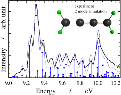
Figure 1: Experimental and calculated (2-mode model) ionization spectra of butatriene (BT), showing nice agreement. See the inset for the equilibrium structure of neutral BT, corresponding to the Franck–Condon point. The calculated spectral lines are convoluted with a Gaussian function of full width at half maximum of $0.05~{}\textrm{eV}$ to account for the experimental resolution.

Fig. 2 shows different PES cuts. It is clearly visible in panel a of Fig. 2 that the two-dimensional adiabatic (cavity-free) PESs of BT⁺ along normal coordinates $Q_{\textrm{t}}$ and $Q_{\textrm{c}}$ form a natural CI at $78447~{}\textrm{cm}^{-1}$ ($9.73~{}\textrm{eV}$) above the minimum of the BT ground state. Panel b of Fig. 2 provides one-dimensional BT⁺ PES cuts along $Q_{\textrm{t}}$ ($Q_{\textrm{c}}=Q_{{}_{\textrm{TDM}}}=Q_{{}_{\textrm{PDM}}}=0$). Besides $V_{\textrm{X}}$ and $V_{\textrm{A}}$ one can also see $V_{\textrm{X}}+\hbar\omega_{\textrm{cav}}$ and $V_{\textrm{A}}+\hbar\omega_{\textrm{cav}}$ in panel b, both shifted by the photon energy with $\omega_{\textrm{cav}}=645.02~{}\textrm{cm}^{-1}$. As indicated in panel b, the natural CI at $Q_{\textrm{t}}=-8.80~{}\sqrt{m_{\textrm{e}}}a_{0}$ (formed between $V_{\textrm{X}}$ and $V_{\textrm{A}}$) is adjacent to the LICI located at $Q_{\textrm{t}}=-7.04~{}\sqrt{m_{\textrm{e}}}a_{0}$ (between $V_{\textrm{X}}+\hbar\omega_{\textrm{cav}}$ and $V_{\textrm{A}}$) in this particular case.

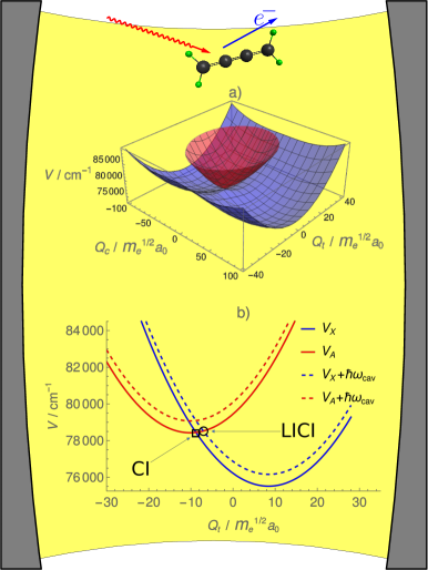
Figure 2: (a) Two-dimensional adiabatic (cavity-free) potential energy surfaces (PESs) of the butatriene cation (BT⁺) along the tuning ($Q_{\textrm{t}}$) and coupling ($Q_{\textrm{c}}$) modes. (b) One-dimensional PES cuts of BT⁺ along $Q_{\textrm{t}}$ with $Q_{\textrm{c}}=Q_{{}_{\textrm{TDM}}}=Q_{{}_{\textrm{PDM}}}=0$. $V_{\textrm{X}}$ and $V_{\textrm{A}}$ refer to the ground-state and excited-state PESs of BT⁺, while $V_{\textrm{X}}+\hbar\omega_{\textrm{cav}}$ and $V_{\textrm{A}}+\hbar\omega_{\textrm{cav}}$ are the same curves shifted by the photon energy with $\omega_{\textrm{cav}}=645.02~{}\textrm{cm}^{-1}$. Positions of the natural conical intersection (CI, between $V_{\textrm{X}}$ and $V_{\textrm{A}}$) and the light-induced conical intersection (LICI, between $V_{\textrm{X}}+\hbar\omega_{\textrm{cav}}$ and $V_{\textrm{A}}$) are explicitly marked in the figure.

The three panels of Fig. 3 show computed ionization spectra within the 4-mode model for $\omega_{\textrm{cav}}=645.02~{}\textrm{cm}^{-1}$ and $g=0.1~{}\textrm{au}$. The results for three different polarizations of the cavity field are depicted in red. For comparison, the ionization spectra of the 4-mode model, but without coupling to the cavity are also depicted in blue. The polarization in panel a is $\mathbf{e}=(0,1,0)$, i.e., along the $y$ axis. In this case, only the PDMs in the electronic states couple the molecule to the cavity and this takes place via the $\nu_{{}_{\textrm{PDM}}}$ mode. In panel b the polarization is along the $x$ axis, $\mathbf{e}=(1,0,0)$, and the coupling is by the $\nu_{{}_{\textrm{TDM}}}$ mode only. The orthogonality of the TDM to the PDMs allows us to control the cavity-induced effects by changing the field polarization and to study the impact of the individual modes on the spectrum. This has been another reason to choose BT as our object for investigation. The joint impact of the PDM and TDM modes can be studied by varying the polarization in the $xy$-plane, an example is shown in panel c for $\mathbf{e}=(1,1,0)/\sqrt{2}$. In each case, the system is initially assumed to be in the vibrational ground state of BT with zero photons in the cavity which corresponds to the lowest eigenstate of the coupled cavity-molecule system to a very good approximation.

As already stated, due to high symmetry, the original 2-mode vibrational model is insufficient to account for cavity-molecule interactions. However, by moving away from the FC point along modes $\nu_{{}_{\textrm{TDM}}}$ and $\nu_{{}_{\textrm{PDM}}}$ the TDM and PDM values are no longer zero and consequently, BT⁺ can interact with the cavity mode. More precisely, the coupling to the cavity is induced by dynamical symmetry breaking activated by the process of ionization in the cavity. The impact of the cavity on the ionization process is seen to strongly depend on the orientation of the molecule with respect to the field polarization. Accordingly, besides the original $\nu_{\textrm{c}}$ coupling and $\nu_{\textrm{t}}$ tuning modes (which span the cavity-free branching space), $\nu_{{}_{\textrm{PDM}}}$ (only PDM, panel a of Fig. 3), $\nu_{{}_{\textrm{TDM}}}$ (only TDM, panel b), or both $\nu_{{}_{\textrm{TDM}}}$ and $\nu_{{}_{\textrm{PDM}}}$ (panel c) come into play. It is conspicuous in Fig. 3 that the cavity-free (blue) and cavity (red) spectra can differ considerably from each other as seen in panels a (only PDM) and c. The impact of $\nu_{{}_{\textrm{TDM}}}$ (panel b) is found to be rather minor in BT⁺. These observations are attributed to the strong mixing by the PDMs of the vibrational levels of the surfaces originating from the solid and dashed blue curves and those originating from the respective red curves in Fig. 2. The resulting hybrid light-matter states are subject to the electronic mixing imposed by the natural CI and are, therefore, expected to strongly change the nonadiabatic effects found in the cavity-free case. Indeed, it is seen in panel a that intense lines in the cavity-free spectrum above about $9.55~{}\textrm{eV}$ (blue) are split into many lines of tiny intensities (red).

The energetic position of the natural CI is $9.55~{}\textrm{eV}$ above the zero-point energy of BT. Thus, following Ref. 57, the original cavity-free spectrum can be divided into adiabatic ($E<9.55~{}\textrm{eV}$) and nonadiabatic ($E>9.55~{}\textrm{eV}$) regions. It is apparent in Fig. 3 that the nonadiabatic region is significantly modified by the cavity, while the adiabatic region remains largely unaffected by cavity-molecule interactions (some levels do mix in, but their energy splittings are seen to be very small). This finding can be rationalized in the following way. Nonzero cavity-molecule couplings and cavity effects in the ionization spectrum can be ascribed to dynamical symmetry breaking induced by displacement along modes $\nu_{{}_{\textrm{TDM}}}$ and $\nu_{{}_{\textrm{PDM}}}$. Owing to the conditions required by the LICI formation (degenerate diabatic potentials and zero cavity-molecule couplings) the LICI is situated in the vicinity of the natural CI for $\omega_{\textrm{cav}}=645.02~{}\textrm{cm}^{-1}$ (see panel b of Fig. 2). As a result, the natural CI and the LICI start exerting their effects roughly above the same energy and imprint their signatures in the nonadiabatic region of the cavity-free ionization spectrum, including the mystery band which (itself) emerges due to natural nonadiabatic effects. Several additional ionization spectra have been computed, supporting our conclusions. Two of them are shown as examples in the Supplemental Material.

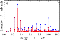
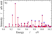
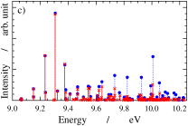
Figure 3: Cavity-free (blue, $\bullet$) and cavity (red, x) ionization spectra of butatriene with cavity parameters $\omega_{\textrm{cav}}=645.02~{}\textrm{cm}^{-1}$ and $g=0.1~{}\textrm{au}$. The field polarization vector is chosen in three different ways: $\mathbf{e}=(0,1,0)$ (panel a, only permanent dipole moments (PDMs)), $\mathbf{e}=(1,0,0)$ (panel b, only transition dipole moment (TDM)), and $\mathbf{e}=(1,1,0)/\sqrt{2}$ (panel c, both TDM and PDMs). Significant cavity-induced dynamical effects can be observed mainly in the nonadiabatic region (above $9.55~{}\textrm{eV}$) of the ionization spectrum.

We would like to point out that the natural CI appears again between the surfaces originating from the two dashed curves and the same holds for the LICI which appears again between the red dashed and the blue solid curves (see Fig. 2). This second “natural CI” is actually also a light-induced CI as it does not exist without the cavity. Owing to the low value of the cavity frequency employed, the nonadiabatic effects discussed above are due to all of these four conical intersections.

In contrast to BT⁺, many typical molecules possess nonzero TDM and/or PDM values at the FC point. In such cases, there is no need to dynamically break the symmetry of the molecule in order to achieve a strong impact of the cavity on the ionization spectrum. Consequently, the ionization spectrum is expected to show striking cavity-induced effects which one may call static effects, meaning that no dynamical symmetry breaking is involved. In order to demonstrate the emergence of static effects in the ionization spectrum, constant TDM (along the $x$ axis) and PDM (along the $y$ axis) values of $1.0~{}\textrm{au}$ are added artificially to the original 2-mode model of BT⁺. Fig. 4 presents cavity ionization spectra for the modified 2-mode model with cavity parameters $\omega_{\textrm{cav}}=645.02~{}\textrm{cm}^{-1}$ and $g=0.002~{}\textrm{au}$ (panel a), and $\omega_{\textrm{cav}}=3000.0~{}\textrm{cm}^{-1}$ and $g=0.01~{}\textrm{au}$ (panel b), both obtained with $\mathbf{e}=(1,1,0)/\sqrt{2}$ (both TDM and PDMs are included). As clearly visible in Fig. 4, cavity-induced effects are more pronounced than in Fig. 3 and they affect the entire energy range of the ionization spectra, including the adiabatic region. These observations are remarkable in light of the much lower coupling strengths $g=0.002~{}\textrm{au}$ and $g=0.01~{}\textrm{au}$ (used in Fig. 4) compared to $g=0.1~{}\textrm{au}$ (used in Fig. 3).

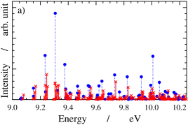
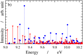
Figure 4: Cavity-free (blue, $\bullet$) and cavity (red, x) ionization spectra of butatriene with cavity parameters $\omega_{\textrm{cav}}=645.02~{}\textrm{cm}^{-1}$, $g=0.002~{}\textrm{au}$ (panel a), and $\omega_{\textrm{cav}}=3000.0~{}\textrm{cm}^{-1}$, $g=0.01~{}\textrm{au}$ (panel b). In this case, constant transition (TDM, along the $x$ axis) and permanent (PDM, along the $y$ axis) dipole moment values of $1.0~{}\textrm{au}$ are added to the 2-mode model. The field polarization is chosen as $\mathbf{e}=(1,1,0)/\sqrt{2}$ (both TDM and PDMs). Significant cavity-induced static effects can be observed in the entire spectral range.

This letter discusses the effect of cavity on molecular ionization spectra. To the best of our knowledge, this is the first study to explore striking cavity-induced effects in the low-energy ionization spectrum of molecules. The system of interest is the butatriene cation, BT⁺, which possesses a natural CI between its ground and first excited electronic states near the Franck–Condon (FC) region of the neutral molecule. The natural CI yields a well-separated band, termed the “mystery band”, in the cavity-free ionization spectrum. The 2-mode vibronic coupling model treating a coupling and a tuning vibrational mode has been shown to reproduce the cavity-free low-energy ionization spectrum with good accuracy.[67] However, the 2-mode model is incapable of describing cavity-molecule interactions as the transition (TDM) and permanent (PDM) dipole moments are identically zero at the FC point as well as in the subspace spanned by the coupling and tuning modes. In order to generate cavity-molecule interactions, one needs to break the symmetry of BT⁺ by making displacements along two additional modes to yield nonzero TDM and PDM values. This symmetry breaking takes place by the dynamics of the system after ionization and causes noticeable changes primarily in the nonadiabatic region of the ionization spectrum (that is, above the energetic position of the natural CI). This impact of the cavity on the nonadiabatic regime is explained by the proximity of the light-induced CI (LICI) to the natural CI. Our example, butatriene, has been chosen because of its high symmetry which allows for a transparent discussion of the emerging effects. However, it is often the case that molecules possess nonzero TDM and/or PDMs at the FC point. In this case static cavity-induced effects (involving no dynamical symmetry breaking) are expected to give rise to enormous changes in the entire range of the ionization spectrum. Such effects have been demonstrated for a modified 2-mode model with constant TDM and PDM functions.

Supplemental Material

I Description of the molecule and group-theoretical considerations

The planar equilibrium structure of butatriene (Franck–Condon (FC) point), shown in Fig. 5, is of $D_{2\textrm{h}}$ symmetry. The character table of the $D_{2\textrm{h}}$ point group is provided in Table 1. The two lowest electronic states X and A of the cation have $\Gamma_{\textrm{X}}=B_{2\textrm{g}}$ and $\Gamma_{\textrm{A}}=B_{2\textrm{u}}$ symmetries at the FC point, respectively. Following Ref. 67, the 18 vibrational modes of butatriene can be classified by $D_{2\textrm{h}}$ irreducible representations (irreps) as

$$\Gamma_{\textrm{vib}}=4A_{\textrm{g}}\oplus A_{\textrm{u}}\oplus 2B_{2\textrm{g}}\oplus 3B_{3\textrm{g}}\oplus 3B_{1\textrm{u}}\oplus 3B_{2\textrm{u}}\oplus 2B_{3\textrm{u}}.$$ (3)

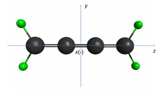
Figure 5: Equilibrium structure of the neutral butatriene (C₄H₄) molecule and definition of the body-fixed Cartesian axes. The minus sign indicates that the $x$ axis is directed inward.

Table 1: Character table of the $D_{2\textrm{h}}$ point group.

	$E$	$C_{2}(z)$	$C_{2}(y)$	$C_{2}(x)$	$i$	$\sigma(xy)$	$\sigma(xz)$	$\sigma(yz)$
$A_{\textrm{g}}$	1	1	1	1	1	1	1	1
$B_{1\textrm{g}}$	1	1	$-1$	$-1$	1	1	$-1$	$-1$
$B_{2\textrm{g}}$	1	$-1$	1	$-1$	1	$-1$	1	$-1$
$B_{3\textrm{g}}$	1	$-1$	$-1$	1	1	$-1$	$-1$	1
$A_{\textrm{u}}$	1	1	1	1	$-1$	$-1$	$-1$	$-1$
$B_{1\textrm{u}}$	1	1	$-1$	$-1$	$-1$	$-1$	1	1
$B_{2\textrm{u}}$	1	$-1$	1	$-1$	$-1$	1	$-1$	1
$B_{3\textrm{u}}$	1	$-1$	$-1$	1	$-1$	1	1	$-1$

Using the body-fixed axis definitions in Fig. 5, we get that the $x$, $y$ and $z$ coordinates transform according to the irreps

$$\Gamma_{x}=B_{3\textrm{u}}\qquad\Gamma_{y}=B_{2\textrm{u}}\qquad\Gamma_{z}=B_{1\textrm{u}}.$$ (4)

Since the direct product representations

$$\Gamma_{\textrm{X}}\otimes\Gamma_{x}\otimes\Gamma_{\textrm{A}}=B_{2\textrm{g}}\otimes B_{3\textrm{u}}\otimes B_{2\textrm{u}}=B_{3\textrm{g}}$$

$$\Gamma_{\textrm{X}}\otimes\Gamma_{y}\otimes\Gamma_{\textrm{A}}=B_{2\textrm{g}}\otimes B_{2\textrm{u}}\otimes B_{2\textrm{u}}=B_{2\textrm{g}}$$ (5)

$$\Gamma_{\textrm{X}}\otimes\Gamma_{z}\otimes\Gamma_{\textrm{A}}=B_{2\textrm{g}}\otimes B_{1\textrm{u}}\otimes B_{2\textrm{u}}=B_{1\textrm{g}}$$

do not contain the totally symmetric irrep $A_{\textrm{g}}$, all components of the transition dipole moment (TDM) between the $\textrm{X}~{}^{2}B_{2\textrm{g}}$ and $\textrm{A}~{}^{2}B_{2\textrm{u}}$ states vanish at the FC point. Using similar arguments one can easily show that the $\textrm{X}~{}^{2}B_{2\textrm{g}}$ and $\textrm{A}~{}^{2}B_{2\textrm{u}}$ permanent dipole moments (PDMs) are also zero at the FC point, for example, one gets

$$\Gamma_{\textrm{X}}\otimes\Gamma_{x}\otimes\Gamma_{\textrm{X}}=B_{2\textrm{g}}\otimes B_{3\textrm{u}}\otimes B_{2\textrm{g}}=B_{3\textrm{u}}$$

$$\Gamma_{\textrm{X}}\otimes\Gamma_{y}\otimes\Gamma_{\textrm{X}}=B_{2\textrm{g}}\otimes B_{2\textrm{u}}\otimes B_{2\textrm{g}}=B_{2\textrm{u}}$$ (6)

$$\Gamma_{\textrm{X}}\otimes\Gamma_{z}\otimes\Gamma_{\textrm{X}}=B_{2\textrm{g}}\otimes B_{1\textrm{u}}\otimes B_{2\textrm{g}}=B_{1\textrm{u}}$$

for the $\textrm{X}~{}^{2}B_{2\textrm{g}}$ state.

It is evident from Eq. (5) that displacement along a given $B_{3\textrm{g}}$ or $B_{2\textrm{g}}$ vibrational mode has to be made to produce nonzero TDM along the body-fixed $x$ and $y$ axes, respectively. Since according to Eq. (3) there is no $B_{1\textrm{g}}$ mode, simultaneous displacements along a $B_{3\textrm{g}}$ and a $B_{2\textrm{g}}$ mode are required to produce TDM along the body-fixed $z$ axis. Similar rules can be derived for PDM components along the same lines, namely, displacements along $B_{3\textrm{u}}$, $B_{2\textrm{u}}$ and $B_{1\textrm{u}}$ modes generate PDMs along the body-fixed $x$, $y$ and $z$ axes, respectively.

Finally, vibrational modes relevant for the current study are described in Table 2. As discussed in the next section, the modes $\nu_{14}$ and $\nu_{5}$ play the role of the tuning ($\nu_{\textrm{t}}$) and coupling ($\nu_{\textrm{c}}$) modes, respectively. In addition to $\nu_{\textrm{t}}$ and $\nu_{\textrm{c}}$, we choose modes $\nu_{9}$ ($\nu_{{}_{\textrm{TDM}}}$) and $\nu_{10}$ ($\nu_{{}_{\textrm{PDM}}}$) to generate TDM and PDMs along the $x$ and $y$ axes. This way, $\nu_{{}_{\textrm{TDM}}}$ and $\nu_{{}_{\textrm{PDM}}}$ give rise to cavity-molecule couplings upon displacement from the FC point.

Table 2: Experimental ($\omega_{\textrm{exp}}$) and calculated ($\omega_{\textrm{calc}}$, MP2/D95** level of theory) harmonic wavenumbers in units of $\textrm{cm}^{-1}$, symmetry labels ($D_{2\textrm{h}}$ point group) and qualitative descriptions of the vibrational modes relevant for the current study. Harmonic wavenumbers used in numerical computations are set in bold.

mode	symmetry	$\omega_{\textrm{exp}}~{}/~{}\textrm{cm}^{-1}$	$\omega_{\textrm{calc}}~{}/~{}\textrm{cm}^{-1}$	description
$\nu_{14}$	$A_{\textrm{g}}$	$\mathbf{2079.30}$	$2157.27$	C–C stretch (central)
$\nu_{5}$	$A_{\textrm{u}}$	$\mathbf{735.58}$	$777.57$	torsion
$\nu_{9}$	$B_{3\textrm{g}}$	$662.99$	$\mathbf{1014.34}$	CH2 rocking
$\nu_{10}$	$B_{2\textrm{u}}$	$\mathbf{1059.81}$	$1050.12$	CH2 rocking

II Description of the 2-mode vibronic coupling model

In this section the 2-mode vibronic coupling model is briefly summarized where vibrational modes $\nu_{5}$ and $\nu_{14}$ correspond to the coupling ($\nu_{\textrm{c}}$) and tuning ($\nu_{\textrm{t}}$) modes, respectively. The ground electronic state of the neutral molecule is described by the harmonic oscillator Hamiltonian

$$\hat{H}_{0}^{\textrm{neutral,2D}}=\hat{T}+V$$ (7)

with

$$\hat{T}=-\frac{1}{2}\sum_{i=\textrm{c},\textrm{t}}\frac{\partial^{2}}{\partial Q_{i}^{2}}$$ (8)

and

$$V=\frac{1}{2}\sum_{i=\textrm{c},\textrm{t}}\omega_{i}^{2}Q_{i}^{2}$$ (9)

where $Q_{\textrm{c}}$ and $Q_{\textrm{t}}$ refer to normal coordinated associated with the coupling and tuning modes, respectively and $\hbar$ is set to one. The ground (X) and first excited (A) electronic states are taken into account for the cation, which yields the diabatic Hamiltonian

$$\hat{H}_{0}^{\textrm{ion,2D}}=\begin{bmatrix}\hat{T}&0\\ 0&\hat{T}\end{bmatrix}+\begin{bmatrix}V_{\textrm{X}}&V_{\textrm{XA}}\\ V_{\textrm{XA}}&V_{\textrm{A}}\end{bmatrix}$$ (10)

with

$$V_{\textrm{X}}=\epsilon_{\textrm{X}}+\frac{1}{2}\sum_{i=\textrm{c},\textrm{t}}\omega_{i}^{2}Q_{i}^{2}+\kappa_{\textrm{X}}Q_{\textrm{t}},$$ (11)

$$V_{\textrm{A}}=\epsilon_{\textrm{A}}+\frac{1}{2}\sum_{i=\textrm{c},\textrm{t}}\omega_{i}^{2}Q_{i}^{2}+\kappa_{\textrm{A}}Q_{\textrm{t}}$$ (12)

and

$$V_{\textrm{XA}}=\lambda Q_{\textrm{c}}.$$ (13)

The model parameters ($\epsilon_{\textrm{X/A}}$, $\omega_{i}$, $\kappa_{\textrm{X/A}}$, $\lambda$) have been taken from Ref. 67.

Next, a numerical method is presented for solving the eigenproblem of $\hat{H}_{0}^{\textrm{ion,2D}}$. The eigenstates of $\hat{H}_{0}^{\textrm{ion,2D}}$ are expressed as two-component vectors, that is,

$$|\vec{\psi}(Q_{\textrm{c}},Q_{\textrm{t}})\rangle=\begin{bmatrix}|\psi_{\textrm{X}}(Q_{\textrm{c}},Q_{\textrm{t}})\rangle\\ |\psi_{\textrm{A}}(Q_{\textrm{c}},Q_{\textrm{t}})\rangle\end{bmatrix}$$ (14)

which is equivalent to the expansion $|\psi(Q_{\textrm{c}},Q_{\textrm{t}})\rangle=|\psi_{\textrm{X}}(Q_{\textrm{c}},Q_{\textrm{t}})\rangle|\textrm{X}\rangle+|\psi_{\textrm{A}}(Q_{\textrm{c}},Q_{\textrm{t}})\rangle|\textrm{A}\rangle$. Components of $|\vec{\psi}(Q_{\textrm{c}},Q_{\textrm{t}})\rangle$ can be expanded in a product basis of 1D harmonic-oscillator eigenfunctions of the neutral ground state,

$$|\psi_{\alpha}(Q_{\textrm{c}},Q_{\textrm{t}})\rangle=\sum_{v_{\textrm{c}},v_{\textrm{t}}}c^{\alpha}_{v_{\textrm{c}},v_{\textrm{t}}}|\varphi_{v_{\textrm{c}}}(Q_{\textrm{c}})\rangle|\varphi_{v_{\textrm{t}}}(Q_{\textrm{t}})\rangle$$ (15)

with $\alpha=\textrm{X},\textrm{A}$. Matrix elements of $\hat{H}_{0}^{\textrm{ion,2D}}$ in the basis defined in Eq. (15) read

$$\langle\varphi_{v^{\prime}_{\textrm{c}}}\varphi_{v^{\prime}_{\textrm{t}}}|\hat{T}+V_{\alpha}|\varphi_{v_{\textrm{c}}}\varphi_{v_{\textrm{t}}}\rangle=\left[\epsilon_{\alpha}+\omega_{\textrm{c}}\left(v_{\textrm{c}}+\frac{1}{2}\right)+\omega_{\textrm{t}}\left(v_{\textrm{t}}+\frac{1}{2}\right)\right]\delta_{v^{\prime}_{\textrm{c}},v_{\textrm{c}}}\delta_{v^{\prime}_{\textrm{t}},v_{\textrm{t}}}$$

$$+\kappa_{\alpha}\langle\varphi_{v^{\prime}_{\textrm{t}}}|Q_{\textrm{t}}|\varphi_{v_{\textrm{t}}}\rangle\delta_{v^{\prime}_{\textrm{c}},v_{\textrm{c}}}$$ (16)

for the diagonal blocks ($\alpha=\textrm{X},\textrm{A}$) and

$$\langle\varphi_{v^{\prime}_{\textrm{c}}}\varphi_{v^{\prime}_{\textrm{t}}}|V_{\textrm{XA}}|\varphi_{v_{\textrm{c}}}\varphi_{v_{\textrm{t}}}\rangle=\lambda\langle\varphi_{v^{\prime}_{\textrm{c}}}|Q_{\textrm{c}}|\varphi_{v_{\textrm{c}}}\rangle\delta_{v^{\prime}_{\textrm{t}},v_{\textrm{t}}}$$ (17)

for the offdiagonal block of $\hat{H}_{0}^{\textrm{ion,2D}}$. In Eq. (17), coordinate matrix elements for the coupling mode can be obtained as

$$\langle\varphi_{v^{\prime}_{\textrm{c}}}|Q_{\textrm{c}}|\varphi_{v_{\textrm{c}}}\rangle=\frac{1}{\sqrt{2\omega_{\textrm{c}}}}\left(\sqrt{v_{\textrm{c}}+1}\,\delta_{v^{\prime}_{\textrm{c}},v_{\textrm{c}+1}}+\sqrt{v_{\textrm{c}}}\,\delta_{v^{\prime}_{\textrm{c}},v_{\textrm{c}-1}}\right).$$ (18)

Coordinate matrix elements for the tuning mode in Eq. (16) can be expressed in the same fashion.

Finally, a brief description of the computation of the ionization spectrum is provided. The initial state is assumed to be the vibrational ground state of the neutral molecule in its electronic ground state,

$$|\psi_{\textrm{i}}(Q_{\textrm{c}},Q_{\textrm{t}})\rangle=|\varphi_{0}(Q_{\textrm{c}})\rangle|\varphi_{0}(Q_{\textrm{t}})\rangle$$ (19)

where the harmonic-oscillator approximation is applied, see Eq. (7). The final states correspond to eigenstates $|\vec{\psi}_{\textrm{f}}(Q_{\textrm{c}},Q_{\textrm{t}})\rangle$ of the cation defined in Eq. (14). Assuming that ionization probabilities of the neutral ground state are nuclear-position independent and equal for the cationic states X and A we get

$$A_{\textrm{if}}=\sum_{\alpha=\textrm{X},\textrm{A}}\langle\psi_{\textrm{i}}(Q_{\textrm{c}},Q_{\textrm{t}})|\psi_{\textrm{f},\alpha}(Q_{\textrm{c}},Q_{\textrm{t}})\rangle$$ (20)

for the transition amplitudes. Transition probabilities $I_{\textrm{if}}$ are proportional to transition wavenumbers $\omega_{\textrm{if}}$ and absolute squares of transition amplitudes $A_{\textrm{if}}$, that is, $I_{\textrm{if}}\propto\omega_{\textrm{if}}|A_{\textrm{if}}|^{2}$.

III Description of the 4-mode model for the coupled cavity-molecule system

The Hamiltonian of the cation coupled to a single cavity mode has the form

$$\hat{H}_{\textrm{cm}}=\hat{H}_{0}^{\textrm{ion}}+\hbar\omega_{\textrm{cav}}\hat{a}^{\dagger}\hat{a}-g\hat{\vec{\mu}}\vec{e}(\hat{a}^{\dagger}+\hat{a})$$ (21)

which, taking into account the two lowest electronic states (X and A), can be recast as

where $\omega_{\textrm{cav}}$, $g$, $\hat{\vec{\mu}}$ and $\vec{e}$ are the cavity angular frequency, coupling strength parameter, electric dipole moment of the molecule and polarization vector of the cavity field, respectively, while $\hat{a}^{\dagger}$ and $\hat{a}$ denote creation and annihilation operators of the cavity mode. In addition, PDM and TDM components along $\vec{e}$ are denoted by $\mu_{\alpha}$ ($\alpha=\textrm{X},\textrm{A}$) and $\mu_{\textrm{XA}}$, respectively.

In order to produce nonzero TDM and PDMs, $\hat{H}_{0}^{\textrm{ion,2D}}$ of Eq. (10) is supplemented with two additional vibrational modes, which yields

$$\hat{H}_{0}^{\textrm{ion}}=\begin{bmatrix}\hat{T}&0\\ 0&\hat{T}\end{bmatrix}+\begin{bmatrix}V_{\textrm{X}}&V_{\textrm{XA}}\\ V_{\textrm{XA}}&V_{\textrm{A}}\end{bmatrix}$$ (23)

with

$$\hat{T}=-\frac{1}{2}\sum_{\begin{subarray}{c}i=\textrm{c},\textrm{t},\\ \textrm{TDM},\textrm{PDM}\end{subarray}}\frac{\partial^{2}}{\partial Q_{i}^{2}},$$ (24)

$$V_{\textrm{X}}=\epsilon_{\textrm{X}}+\frac{1}{2}\sum_{\begin{subarray}{c}i=\textrm{c},\textrm{t},\\ \textrm{TDM},\textrm{PDM}\end{subarray}}\omega_{i}^{2}Q_{i}^{2}+\kappa_{\textrm{X}}Q_{\textrm{t}},$$ (25)

$$V_{\textrm{A}}=\epsilon_{\textrm{A}}+\frac{1}{2}\sum_{\begin{subarray}{c}i=\textrm{c},\textrm{t},\\ \textrm{TDM},\textrm{PDM}\end{subarray}}\omega_{i}^{2}Q_{i}^{2}+\kappa_{\textrm{A}}Q_{\textrm{t}}$$ (26)

and

$$V_{\textrm{XA}}=\lambda Q_{\textrm{c}}.$$ (27)

The group-theoretical analysis presented in Section I suggests that the PDM and TDM functions can be approximated by the expansions

$$\mu_{\textrm{X}}=\beta_{\textrm{X}}Q_{{}_{\textrm{PDM}}}$$

$$\mu_{\textrm{A}}=\beta_{\textrm{A}}Q_{{}_{\textrm{PDM}}}$$ (28)

$$\mu_{\textrm{XA}}=\gamma Q_{{}_{\textrm{TDM}}}$$

where $\beta_{\textrm{X}}$, $\beta_{\textrm{A}}$ and $\gamma$ are constants.

Eigenstates of the coupled cavity-molecule system are constructed as

$$|\vec{\Phi}_{k}\rangle=\begin{bmatrix}\sum_{\mathbf{v}}\sum_{n}b^{\textrm{X},k}_{\mathbf{v},n}|\mathbf{v}\rangle|n\rangle\\ \sum_{\mathbf{v}}\sum_{n}b^{\textrm{A},k}_{\mathbf{v},n}|\mathbf{v}\rangle|n\rangle\end{bmatrix}$$ (29)

where $|n\rangle$ refers to Fock states of the cavity mode and $|\mathbf{v}\rangle=|v_{\textrm{c}},v_{\textrm{t}},v_{{}_{\textrm{TDM}}},v_{{}_{\textrm{PDM}}}\rangle$ denotes four-dimensional harmonic-oscillator basis states. The matrix representation of $\hat{H}_{\textrm{cm}}$ (see Eq. (22)) is set up using the basis defined in Eq. (29) and the resulting Hamiltonian matrix is diagonalized with a sparse eigensolver. Regarding the ionization spectrum, the initial state is assumed to be the vibrational ground state of the neutral molecule in its electronic ground state with zero photons in the cavity, that is,

$$|\Phi_{0}\rangle=|\mathbf{0}\rangle|0\rangle.$$ (30)

With these quantities at hand transition amplitudes from $|\Phi_{0}\rangle$ to $|\vec{\Phi}_{k}\rangle$ (see Eq. (29)) are expressed as

$$A_{0k}= \sum_{\alpha=\textrm{X},\textrm{A}}\langle\Phi_{0}|\Phi_{k,\alpha}\rangle.$$ (31)

IV Technical details of the computations

IV.1 Ab initio calculations and model parameters

Following Ref. 67, the equilibrium geometry of neutral butatriene was optimized at the MP2/D95** level of theory with the Gaussian 16 program. Normal coordinates were constructed by diagonalizing the mass-weighted Cartesian Hessian and used in subsequent nuclear motion computations. Vibrational modes relevant for the current study are summarized in Table 2 where harmonic wavenumbers used in numerical computations are set in bold. Other model parameters, taken from Ref. 67, are as follows: $\epsilon_{\textrm{X}}=9.45~{}\textrm{eV}$, $\epsilon_{\textrm{A}}=9.85~{}\textrm{eV}$, $\kappa_{\textrm{X}}=-0.212~{}\textrm{eV}$, $\kappa_{\textrm{A}}=0.255~{}\textrm{eV}$ and $\lambda=0.318~{}\textrm{eV}$ ($\kappa_{\textrm{X}}$, $\kappa_{\textrm{A}}$ and $\lambda$ are consistent with dimensionless normal coordinates).

The electronic states X and A of the butatriene cation were obtained at the MRCI/cc-pVTZ level of theory. First, ROHF orbitals were calculated, then state-averaged CASSCF(5,4) computations were carried out using equal weights for the two cationic states with 11 closed-shell orbitals and 4 active orbitals. The final step involved the internally-contracted MRCI method implemented in the Molpro program (version 2020.2). Permanent and transition dipole moments, needed to construct the Hamiltonian of Eq. (22), were obtained at several different nuclear configurations.

IV.2 Diabatic representation of the permanent and transition dipole moment surfaces

As the system is described using the diabatic representation, we need to construct the diabatic PDM and TDM surfaces. This can be achieved by diagonalizing the diabatic potential energy matrix of Eq. (23) for each nuclear configuration,

$$\mathbf{U}^{\textrm{T}}\begin{bmatrix}V_{\textrm{X}}&V_{\textrm{XA}}\\ V_{\textrm{XA}}&V_{\textrm{A}}\end{bmatrix}\mathbf{U}=\begin{bmatrix}V_{\textrm{lower}}&0\\ 0&V_{\textrm{upper}}\end{bmatrix}$$ (32)

which results in the transformation matrix $\mathbf{U}$ and lower and upper adiabatic PESs ($V_{\textrm{lower}}$ and $V_{\textrm{upper}}$). Since ab initio calculations presented in the previous subsection yield PDM and TDM surfaces in the adiabatic representation, the transformation

$$\begin{bmatrix}\mu_{\textrm{X}}&\mu_{\textrm{XA}}\\ \mu_{\textrm{XA}}&\mu_{\textrm{A}}\end{bmatrix}=\mathbf{U}\begin{bmatrix}\mu^{\textrm{ad}}_{\textrm{X}}&\mu^{\textrm{ad}}_{\textrm{XA}}\\ \mu^{\textrm{ad}}_{\textrm{XA}}&\mu^{\textrm{ad}}_{\textrm{A}}\end{bmatrix}\mathbf{U}^{\textrm{T}}$$ (33)

is invoked to construct the diabatic PDM ($\mu_{\textrm{X}}$ and $\mu_{\textrm{A}}$) and TDM ($\mu_{\textrm{XA}}$) surfaces.

As already discussed in Section I, the diabatic PDM and TDM surfaces can be approximated by first-order Taylor expansion about the FC point,

$$\mu_{\textrm{X}}=\left(\frac{\partial\mu_{\textrm{X}}}{\partial Q_{{}_{\textrm{PDM}}}}\right)\bigg{|}_{\textrm{FC}}Q_{{}_{\textrm{PDM}}}=\beta_{\textrm{X}}Q_{{}_{\textrm{PDM}}}$$

$$\mu_{\textrm{A}}=\left(\frac{\partial\mu_{\textrm{A}}}{\partial Q_{{}_{\textrm{PDM}}}}\right)\bigg{|}_{\textrm{FC}}Q_{{}_{\textrm{PDM}}}=\beta_{\textrm{A}}Q_{{}_{\textrm{PDM}}}$$ (34)

$$\mu_{\textrm{XA}}=\left(\frac{\partial\mu_{\textrm{XA}}}{\partial Q_{{}_{\textrm{TDM}}}}\right)\bigg{|}_{\textrm{FC}}Q_{{}_{\textrm{TDM}}}=\gamma Q_{{}_{\textrm{TDM}}}$$

where PDM and TDM derivatives can be estimated by the method of finite differences. Since $\mathbf{U}$ equals the two-dimensional identity matrix in the close vicinity of the FC point, PDM and TDM derivatives in the adiabatic and diabatic representations coincide. Therefore, one can directly use dipole derivatives provided by ab initio calculations: $\beta_{\textrm{X}}=1.05\cdot 10^{-3}~{}\textrm{au}$, $\beta_{\textrm{A}}=-1.89\cdot 10^{-3}~{}\textrm{au}$ and $\gamma=-4.37\cdot 10^{-4}~{}\textrm{au}$, given in atomic units.

V Additional figures

Fig. 6 and Fig. 7 show 4-mode cavity-free (blue) and cavity (red) ionization spectra with $\omega_{\textrm{cav}}=645.02~{}\textrm{cm}^{-1}$ and $g=0.15~{}\textrm{au}$, and $\omega_{\textrm{cav}}=824.80~{}\textrm{cm}^{-1}$ $g=0.1~{}\textrm{au}$, respectively. In both cases, three panels of the figures correspond to the following three different cavity field polarizations (see Fig. 5 for the definition of body-fixed Cartesian axes): $\mathbf{e}=(0,1,0)$ (only PDMs), $\mathbf{e}=(1,0,0)$ (only TDM) and $\mathbf{e}=(1,1,0)/\sqrt{2}$ (both TDM and PDMs).

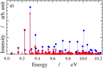
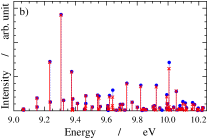
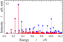
Figure 6: Cavity-free (blue) and cavity (red) ionization spectra of butatriene with cavity parameters $\omega_{\textrm{cav}}=645.02~{}\textrm{cm}^{-1}$ and $g=0.15~{}\textrm{au}$. The field polarization vector is chosen in three different ways: (a) $\mathbf{e}=(0,1,0)$ (only permanent dipole moments (PDMs)), (b) $\mathbf{e}=(1,0,0)$ (only transition dipole moment (TDM)), and (c) $\mathbf{e}=(1,1,0)/\sqrt{2}$ (both TDM and PDMs).

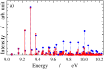
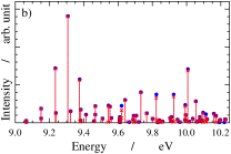
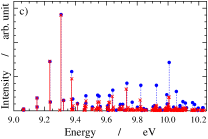
Figure 7: Cavity-free (blue) and cavity (red) ionization spectra of butatriene with cavity parameters $\omega_{\textrm{cav}}=824.80~{}\textrm{cm}^{-1}$ and $g=0.1~{}\textrm{au}$. The field polarization vector is chosen in three different ways: (a) $\mathbf{e}=(0,1,0)$ (only permanent dipole moments (PDMs)), (b) $\mathbf{e}=(1,0,0)$ (only transition dipole moment (TDM)), and (c) $\mathbf{e}=(1,1,0)/\sqrt{2}$ (both TDM and PDMs).