Tracing the assembly histories of galaxy clusters in the nearby universe

Abstract

We have compiled a sample of 67 nearby ($z<$ 0.15) clusters of galaxies, for which on average more than 150 spectroscopic members are available, and, by applying different methods to detect substructures in their galaxy distribution, we have studied their assembly history. Our analysis confirms that substructures are present in 70% of our sample, having a significant dynamical impact in 57% of them. A classification of the assembly state of the clusters based on the dynamical significance of their substructures is proposed. In 19% of our clusters, the originally identified brightest cluster galaxy is not the central gravitationally dominant galaxy (CDG), but turns out to be either the second-rank, or the dominant galaxy of a substructure (a SDG, in our classification), or even a “fossil” galaxy in the periphery of the cluster. Moreover, no correlation was found in general between the projected offset of the CDG from the X-ray peak and its peculiar velocity. The comparison of the CDGs properties with the assembly states and dynamical state of the intracluster media, especially the core cooling status, suggests a complex assembly history, with clear evidence of co-evolution of the CDG and its host cluster in the innermost regions.

Hemos recopilado una muestra de 67 cúmulos cercanos ($z<$ 0.15) de galaxias, para los cuales se dispone de un promedio de más de 150 miembros espectroscópicos, y, aplicando diferentes métodos para detectar subestructuras en su distribución de galaxias, hemos estudiado su historia de ensamblaje. Nuestro análisis confirma la presencia de subestructuras en el 70% de los cúmulos de nuestra muestra, teniendo un impacto dinámico significante en el 57% de ellos. Se propone una clasificación de los estados de ensamblaje de los cúmulos basada en la significancia dinámica de sus subestructuras. En el 19% de nuestros cúmulos, la galaxia más brillante identificada originalmente no es la galaxia gravitacionalmente dominante central (CDG), pero suele ser una segunda galaxia dominante, o la galaxia dominante de una subestructura (una SDG, en nuestra clasificación), o hasta una galaxia “fósil” en la periferia del cúmulo. Además, no se encontró correlación, en general, entre el desplazamiento proyectado de la CDG respecto al pico de emisión en rayos-X y su velocidad peculiar. La comparación de las propiedades de las CDGs con los estados de ensamblaje y estados dinámicos de los medios intracumulares especialmente el estado de enfriamiento del core, sugiere una historia de ensamblaje compleja, con clara evidencia de co-evolución de la CDG y su cúmulo huésped en las regiones más internas.

galaxies: clusters: BCGs galaxies: clusters: membership galaxies: clusters: substructures galaxies: groups: general

0.1 Introduction

According to the hierarchical structure formation paradigm, gravity brings together smaller mass systems into larger, more massive ones: in a sequential process, galaxies assemble in groups, and groups merge to form clusters, which, at the present epoch, have started to congregate over the largest scale appearing as superclusters. At each mass scale, the environment where the object (galaxy, group or cluster) forms influences how it grows and evolves, through complex physical processes that still need to be investigated further and clarified. This makes retracing the assembly histories of such objects/systems a difficult but paramount task.

The effects of the environment on galaxy formation and evolution have been extensively studied (e.g., Dressler, 1980; Caldwell et al., 1993; Poggianti et al., 2006), originally in terms of the cluster-field dichotomy. However, the discussion has recently taken a new turn after realizing that groups and clusters are part of the cosmic web, namely, the large-scale structure (LSS). Within this new paradigm, the global environment of galaxies has a foamy texture, a structure full of voids (e.g., Tempel et al., 2009; Varela et al., 2012; Einasto et al., 2014; Dupuy et al., 2019) that are encircled by a web of filaments (e.g., Porter et al., 2008; Poudel et al., 2017; Santiago-Bautista et al., 2020), where the bulk of the intergalactic gas is found (e.g., Fraser-McKelvie et al., 2011; Planck Collab., 2014; Reiprich et al., 2021), and connected through nodes, where the density of matter is highest. It is along the backbone of the filaments that groups of galaxies form, before migrating and merging within rich clusters of galaxies in the nodes.

Information about the fundamental properties of these structures and their member galaxies has also improved significantly thanks to many surveys: large-scale redshift surveys (e.g., Shectman et al., 1996; Da Costa et al., 1998; Falco et al., 1999; Cole et al., 2005; Jones et al., 2009; Baldry et al., 2010; Huchra et al., 2012; Albareti et al., 2017), optical CCD-based photometric surveys (e.g., Hambly et al., 2001a; Skrutskie et al., 2006; Aihara et al., 2011; Shanks et al., 2015; Dey, 2019; Chambers et al., 2019; Abbott et al., 2021), and interferometric radio surveys (e.g., Becker et al., 1995; Condon et al., 1998; Barnes et al., 2001; Lacy et al., 2020). These studies allowed various physical processes for the formation and evolution of galaxies to be identified, with efficiencies varying with the density of the environments of structures on different scales. Fundamentally, this has shown that understanding how galaxies form and evolve requires understanding how the structure and characteristics of their environments affect their intrinsic properties: their mass, morphology, star formation history and even BH formation and AGN activity.

However, this also implies being able to distinguish environmental effects from those related to secular evolution (the question of whether this is due to “nature or nurture”). A panoply of galaxy characteristics are used to achieve this goal, like their colors, their shapes, their orientations and spins, or equivalent parameters extracted from comparing their spectra with synthetic stellar population models. When studying groups and clusters, distinguishing between nature and nurture also necessitates recognizing the dynamical states of these systems, as reflected by the different distributions of galaxies, intergalactic gas (intracluster medium, ICM, or intragroup medium, IGM) and dark matter (the so-called halo-occupation problem). Reconciling all these different aspects is theoretically demanding and observationally expensive, which complicates the task of building a comprehensive model of their formation and evolution.

Usually, studies related to the structure and evolution of galaxy groups and clusters suffer from one or more of the following limitations: i) only projected positional data are used for substructure analyses (e.g., Lopes et al., 2006; Ramella et al., 2007; Wen & Han, 2013); ii) the use of photometric redshifts (e.g., Wen & Han, 2015; Bonjean et al., 2018) –clearly the estimation of redshifts using only photometry has improved a lot during recent years, but photometric redshifts still lack the accuracy to determine cluster membership and dynamical state in the way that is possible with spectroscopic redshifts–; iii) only a small number of member galaxies with spectroscopic redshifts are available (frequently affecting high-redshift cluster studies); iv) many spectroscopic redshifts are available but only for a small number of clusters (e.g., Tyler et al., 2014; Song et al., 2017; Liu et al., 2018); v) cluster samples that are biased in richness and mass, or focused on special aspects, like regularly shaped clusters, dominated by cD galaxies, showing strong X-ray emission or an ICM with strong Sunyaev-Zel’dovich (SZ) signal (e.g., Oegerle & Hill, 2001; Rumbaugh et al., 2018; Lopes et al., 2018). To palliate these limitations, we aim to build a database collecting information related to the environments of different structures in the nearby Universe (from groups to superclusters), that is as complete and homogeneous as possible. In this paper, we concentrate more specifically on defining a sample of galaxy clusters that have a large range of richness, to establish their dynamical and evolutionary states in order to trace their assembly histories.

For that we need to better investigate the importance of substructures and their dynamically dominant galaxies for the cluster evolution as a whole. We make a clear distinction here between the photometric ranking of member galaxies of a galaxy system (cluster or group), which has lead to the terms BCG (Brightest Cluster Galaxy) and BGG (Brightest Group Galaxy), and a ranking that takes into account their dynamical relevance and evolution. Because today we have enough information to study the assembly and evolution of galaxy clusters, this distinction becomes necessary. Thus, we define, for each cluster or group, a CDG (Central Dominant Galaxy), and one or more SDGs (Substructure/Sub-cluster/Satellite Dominant Galaxies) for each of the cluster substructures when they are present. The CDG and SDGs of a cluster are usually the brightest galaxies of this cluster, and we will retain the term BCGs to refer colectivelly to them. In other words, BCGs and BGGs are photometrically defined prior to a dynamical analysis, while CDGs and SDGs are a reclassification of the BCGs and BGGs according to their host sub-systems and dynamical importance.

Moreover, assuming that CDGs with a cD (or D) type morphology form by cannibalizing galaxies falling toward the center of the potential wells of the clusters (e.g., Coziol et al., 2009; Zhao et al., 2015), one would naturally expect their masses to show some specific relation with the masses of their parent structures, $M_{Cl}$–$M_{CDG}$ (e.g., Stott et al., 2010; Lavoie et al., 2016). In particular, we would expect CDGs in dynamically relaxed clusters to lie at the bottom of the potential wells of their systems. However, observations show that, for most of the clusters, the positions of many cDs are offset from the peak in X-ray emission, the latter assumed to settle more rapidly to the bottom of the potential well, or having high peculiar velocities within the cluster compared to the center of the radial velocity distribution (Coziol et al., 2009; Martel et al., 2014; Lauer et al., 2014). This points to most of the clusters being unrelaxed or maybe to the presence of some undetected projection effects.

Another difficulty lies in the cannibalism mechanism itself. How can mergers happen efficiently in a systems where the velocity dispersion of galaxies increases as they fall into deep potential wells (e.g., Merritt, 1985; Tonry, 1985; Mihos, 2004)? Alternatively, an important part of the formation of galaxies now in clusters could have happened in smaller-mass systems, like groups, where the velocity dispersion (and thus the amount of ICM) is smaller, the groups then merging to form or enrich more massive clusters. This phenomenon is known in literature as pre-processing (e.g., Caldwell et al., 1993; Caretta et al., 2008; Donnari et al., 2021).

Within the cosmic web paradigm, one needs to ponder how the constant feeding of clusters by the merging and accretion of groups forming in filaments tempered these expectations. For instance, assuming mergers take place regularly, substructures in the distribution of galaxies would be expected to be common at low redshifts. This would naturally explain the CDG–X-ray offsets, since the ICM having a higher impact parameter than galaxies would follow a different path towards virialization, reaching equilibrium more rapidly.

Common mergers of groups within a cluster would also be expected to disrupt the cool core (CC) of this system, making the CDG wobble around the distorted potential well, explaining its peculiar velocity (e.g., Harvey et al., 2017). This could also have an important impact on the formation of cD galaxies. In the evolution scenario proposed by Lavoie et al. (2016), for example, it is proposed that a CDG transforms into a cD by cannibalism only when, after a cluster-scale merger event, the most massive galaxies of the merging groups, displaced from their initial potential, migrate towards the potential center of the newly formed cluster; this temporary imbalance increases dynamical friction and thus favors cannibalism. Consequently, one would expect the magnitude gaps to increase between the CDG and its luminous neighbors, but not necessarily between the second and third-rank galaxies, due to their high velocity dispersion.

All these considerations suggest that, assuming that groups in filaments continuously merge to form clusters, several primeval group CDGs might appear among the BCGs of a cluster. Moreover, due to the different time-scales for the relaxation of such complex systems, we might also expect the galaxy distributions and characteristics to reflect some specific aspects of their merger processes. By compiling and studying a well characterized sample of galaxy clusters, therefore, it should be possible to distinguish different states of the merger process, and better document their assembly histories.

The sample we present in this article is an effort in this direction. It is composed of 67 optically selected Abell galaxy clusters that are nearby ($z<$ 0.15), and for which a large number (above 100) of spectroscopically confirmed potential members are available. This sample includes a fair distribution of all Bautz-Morgan (BM) type clusters and various levels of ICM X-ray properties (from luminous to under-luminous, AXU). The article is organized in the following way. In § 0.2, we present the data used in our study: we introduce the cluster and galaxy samples and describe the information retrieved from the photometric, astrometric and spectroscopic observations. In § 0.3, we describe the methods we used to characterize the galaxy systems and their structures: center and membership determination, characterization of dynamical parameters (like cluster redshift, velocity dispersion, richness, mass, gravitational binding, and CDG offsets and gaps), and optical substructuring analyses. Our results about the dynamical properties and level of substructuring, for the outer, inner and core regions of the systems, are discussed in § 0.4. This is followed by a brief summary and conclusions in § 0.5. For our analysis, we assume a standard $\Lambda$CDM cosmology, with $\Omega_{\Lambda}=0.7$, $\Omega_{\mathrm{M}}=0.3$ and H${}_{0}=$ 70 $h_{70}$ km s^-1 Mpc^-1.

0.2 Data

0.2.1 Cluster sample

To build our sample of galaxy clusters, we started with the compilation maintained by one of us (Andernach et al. 2005, see also Chow-Martínez et al. 2014), where we included clusters for which at least $N_{z}=100$ spectroscopic-redshifts from the literature were available. These are nearby, optically selected Abell-ACO (Abell et al., 1989) galaxy clusters, with richness varying from poor to rich, and located within the redshift range 0.005 $<z<$ 0.150. In each cluster, a galaxy is identified as potential member when its apparent position puts it inside a projected Abell radius, R_A = 2.14 $h_{70}^{-1}$ Mpc, and its radial velocity has a value within $\pm\ 2\,500$ km s^-1 of a preliminary estimate for the central velocity of the system. However, its final acceptance as member will depend on a more thorough analysis, which is explained in § 0.3.

Our cluster sample is presented in Table LABEL:T_Sample, together with some relevant data taken from the literature. The first seven columns reproduce the original ACO data for the clusters: the cluster ID (col. 1), its equatorial coordinates, RA and Dec, in J2000 (col. 2 and col. 3), its richness ($\cal{R}$ in col. 4), distance class ($\cal{D}$ in col. 5), BM-type (BM in col. 6; Bautz & Morgan, 1970) (we have converted the original scale I, II, III to 1, 3, 5 and intermediate types 2 and 4), and Rood-Sastry type when available (RS in col. 7; Rood & Sastry, 1971; Struble & Rood, 1982). The X-ray characteristics for each cluster are given in columns 8 to 14: alternative X-ray name when existent (col. 8), equatorial coordinates of the X-ray emission peak (centroid position; J2000 RA and Dec in col. 9 and col. 10), the X-ray luminosity inside $r_{500}$ (col. 11; this is the radius at which the mean interior overdensity is 500 times the critical density, $\rho_{c}$, at the respective redshift), $r_{500}$ itself (col. 12; mostly from Piffaretti et al., 2011), and the X-ray temperature as measured by Migkas et al. (2020) in col. 13, or by others as indicated in col. 14. Note that there are new temperatures for four clusters, based on XMM-Newton and Chandra, presented for the first time in this table (see Appendix 0.6). Finally, we list the membership of a cluster in a supercluster (col. 15), based on the Master SuperCluster Catalog (MSCC; Chow-Martínez et al., 2014), followed in col. 16 by an alternate or common name, when available, or the name of the pair when it is the case, and multiplicity, $m$, of the supercluster in col. 17, the multiplicity being the number of Abell clusters forming the supercluster.

This sample is well balanced in terms of BM types, covering all the possible different dynamical states: containing 17, 17, 9, 9 and 15 clusters, respectively with BM types 1 to 5. It also follows roughly the distribution of richness of ACO clusters, clearly favoring low richness systems, in accordance with the power-law mass distribution function for clusters: 20 are classified as $\cal{R}$ = 0 (poorest; 30-49 galaxies), 24 as $\cal{R}$ = 1 (50-79), 20 as $\cal{R}$ = 2 (80-129) but only 2 as $\cal{R}$ = 3 (130-199) and 1 as $\cal{R}\geq$ 4 (richest; more than 200 galaxies). However, due to the spectroscopic selection criterion, the distribution of Abell distance classes ($\cal{D}$ varying from 0 to 7) is not equally represented, favoring nearby clusters.

-1cm-1cm Table 1: Cluster sample. ACO data X-ray data LSS data ACO RA_ACO Dec_ACO $\cal{R}$ $\cal{D}$ BM RS Alt_Name RA_X Dec_X L₅₀₀ $r_{500}$ $k$T_X Ref. MSCC SC_Name $m$ [deg]_J2000 [deg]_J2000 [deg]_J2000 [deg]_J2000 [$10^{44}$ erg/s] [Mpc] [keV] (1) (2) (3) (4) (5) (6) (7) (8) (9) (10) (11) (12) (13) (14) (15) (16) (17) A2798 9.3916 $-$28.5417 1 5 2 – J0037.4-2831 9.3625 $-$28.5311 0.5455 0.7476 3.39 5 33 Scl(C) 24 A2801 9.6404 $-$29.0752 1 6 1 – 9.6346 $-$29.0789 3.20 2 33 Scl(C) 24 A2804 9.9149 $-$28.9088 1 5 2 – 9.9113 $-$28.8892 1.00 8 33 Scl(C) 24 A0085 10.4075 $-$9.3425 1 4 1 cD J0041.8-0918 10.4587 $-$9.3019 5.1001 1.2103 7.23 10 39 PisCet-N 11 A2811 10.5386 $-$28.5426 1 5 2 – J0042.1-2832 10.5363 $-$28.5358 2.7341 1.0355 5.89 10 33 Scl(C) 24 A0118 13.9329 $-$26.4127 1 5 5 I 33 Scl(NE) 24 A0119 14.0890 $-$1.2629 1 3 4 C J0056.3-0112 14.0762 $-$1.2167 1.4372 0.9413 5.82 10 45 - 4 A0122 14.3571 $-$26.2799 1 5 2 B J0057.4-2616 14.3529 $-$26.2806 0.8612 0.8165 3.70 11 33 Scl(NE) 24 A0133 15.6610 $-$21.7982 0 4 1 cD J0102.7-2152 15.6754 $-$21.8736 1.4602 0.9379 4.25 10 27 PisCet-C 9 A2870 16.9299 $-$46.9165 0 3 1 – 1.07 11 41 Phe 8 A2877 17.4554 $-$45.9006 0 2 1 C J0110.0-4555 17.5017 $-$45.9228 0.1815 0.6249 3.28 10 41 Phe 8 A3027 37.6300 $-$33.0953 0 4 5 – J0230.7-3305 37.6812 $-$33.0986 0.4186 0.7200 3.12 5 iso - 1 A0400 44.4107 6.0333 1 1 4 I J0257.6+0600 44.4121 6.0061 0.2211 0.6505 2.25 10 iso Southern GW 1 A0399 44.4851 13.0164 1 3 2 cD J0257.8+1302 44.4575 13.0492 3.5929 1.1169 6.69 10 108 +A0401 2 A0401 44.7373 13.5823 2 3 1 cD J0258.9+1334 44.7396 13.5794 6.0886 1.2421 7.06 10 108 +A0399 2 A3094 47.8608 $-$26.9289 2 4 2 – J0311.4-2653 47.8542 $-$26.8997 0.3343 0.6907 3.15 11 114 - 3 A3095 48.1094 $-$27.1464 0 4 2 – 114 - 3 A3104 48.5788 $-$45.4150 0 4 1 – J0314.3-4525 48.5825 $-$45.4242 1.0275 0.8662 3.56 10 115 HorRet-B 9 S0334 49.0794 $-$45.1168 0 4 3 – 115* HorRet-B 9 S0336 49.3815 $-$44.7012 0 4 3 – 115* HorRet-B 9 A3112 49.4845 $-$44.2349 2 4 1 cD J0317.9-4414 49.4937 $-$44.2389 3.8159 1.1288 5.49 10 115 HorRet-B 9 A0426 49.6517 41.5151 2 0 4 L J0319.7+4130 49.9467 41.5131 6.2174 1.2856 6.42 4 96 PerPis 3 S0373 54.6289 $-$35.4545 0 0 1 C J0338.4-3526 54.6163 $-$35.4483 0.0197 0.4017 1.56 4 iso Southern SC 1 A3158 55.7526 $-$53.6426 2 4 2 – J0342.8-5338 55.7246 $-$53.6353 2.7649 1.0667 5.42 10 117 HorRet-A 26 A0496 68.4045 $-$13.2462 1 3 1 cD J0433.6-1315 68.4100 $-$13.2592 1.8530 0.9974 4.64 10 iso - 1 A0539 79.1463 6.4540 1 2 5 F J0516.6+0626 79.1554 6.4378 0.5377 0.7773 3.04 4 iso - 1 A3391 96.5644 $-$53.6812 0 4 1 – J0626.3-5341 96.5950 $-$53.6956 1.1601 0.8978 5.89 10 160 - 3 A3395 96.8796 $-$54.3994 1 4 2 F J0627.2-5428 96.9000 $-$54.4463 1.3755 0.9298 5.10 7 160 - 3 A0576 110.3506 55.7389 1 2 5 I J0721.3+5547 110.3425 55.7864 0.7571 0.8291 4.27 10 iso - 1 A0634 123.6404 58.0479 0 3 5 F iso - 1 A0754 137.2086 $-$9.6366 2 3 2 cD J0909.1-0939 137.1978 $-$9.6412 3.8497 1.1439 8.93 9 198 +A0780 2 A1060 159.2137 $-$27.5265 1 0 5 C J1036.6-2731 159.1742 $-$27.5244 0.3114 0.7015 2.79 10 365 HyaCen 10 A1367 176.1231 19.8390 2 1 4 F J1144.6+1945 176.1521 19.7589 1.1046 0.9032 3.81 10 295 ComLeo 5 A3526 192.2157 $-$41.3058 0 0 2 F J1248.7-4118 192.1996 $-$41.3078 0.6937 0.8260 3.40 10 365 HyaCen 9 A3530 193.9037 $-$30.3540 0 4 2 – J1255.5-3019 193.8937 $-$30.3306 0.6805 0.8043 3.62 10 389 Shapley(W) 24 A1644 194.3115 $-$17.3535 1 4 3 cD J1257.1-1724 194.2904 $-$17.4003 1.8975 0.9944 5.25 10 370 +A1631 2 A3532 194.3299 $-$30.3702 0 4 4 C J1257.2-3022 194.3204 $-$30.3769 1.3233 0.9201 4.63 10 389 Shapley(W) 24 A1650 194.6926 $-$1.7530 2 5 2 cD J1258.6-0145 194.6712 $-$1.7569 3.4706 1.1015 5.72 10 376 SGW 6 A1651 194.8456 $-$4.1862 1 4 2 cD J1259.3-0411 194.8396 $-$4.1947 3.8536 1.1252 7.47 10 376 SGW 6 A1656 194.9530 27.9807 2 1 3 B J1259.7+2756 194.9296 27.9386 3.4556 1.1378 7.41 10 295 ComLeo 5 A3556 201.0260 $-$31.6605 0 4 1 – 200.9350 $-$31.8380 3.08 6 389 Shapley(C) 24 A1736 201.7173 $-$27.1093 0 2 5 I J1326.9-2710 201.7250 $-$27.1833 1.6675 0.9694 3.34 10 389 Shapley(N) 24 A3558 201.9782 $-$31.4922 4 3 1 – J1327.9-3130 201.9896 $-$31.5025 3.1385 1.1010 5.83 10 389 Shapley(C) 24 A3562 203.3825 $-$31.6729 2 3 1 – J1333.6-3139 203.4012 $-$31.6611 1.3458 0.9265 5.10 10 389 Shapley(C) 24 A1795 207.2522 26.5852 2 4 1 cD J1348.8+2635 207.2208 26.5956 5.4781 1.2236 6.42 10 414 Boo 24 A2029 227.7447 5.7617 2 4 1 cD J1510.9+0543 227.7292 5.7200 8.7267 1.3344 8.45 10 457 - 6 A2040 228.1884 7.4300 1 4 5 C 228.2113 7.4317 2.41 1 454 - 6 A2052 229.1896 7.0003 0 3 2 cD J1516.7+0701 229.1833 7.0186 1.4421 0.9465 2.88 10 458 Her-S 4 A2065 230.6776 27.7226 2 3 5 C J1522.4+2742 230.6104 27.7094 2.6279 1.0480 6.59 10 463 CrB 14 A2063 230.7578 8.6394 1 3 3 cD J1523.0+0836 230.7725 8.6025 1.1388 0.9020 3.34 10 458 Her-S 4 A2142 239.5672 27.2246 2 4 3 B J1558.3+2713 239.5858 27.2269 10.6761 1.3803 11.63 10 472 +A2148 2 A2147 240.5716 15.8954 1 1 5 F J1602.3+1601 240.5779 16.0200 1.3584 0.9351 4.26 10 474 Her-C 5 A2151 241.3125 17.7485 2 1 5 F J1604.5+1743 241.2863 17.7300 0.5088 0.7652 2.10 10 474 Her-C 5 A2152 241.3435 16.4486 1 1 5 F J1605.5+1626 241.3842 16.4419 0.1283 0.5783 2.41 6 474 Her-C 1 A2197 247.0436 40.9072 1 1 5 L J1627.6+4055 246.9175 40.9197 0.0674 0.5093 2.21 3 485 Her-N 4 A2199 247.1540 39.5243 2 1 1 cD J1628.6+3932 247.1583 39.5486 1.9007 1.0040 4.04 10 485 Her-N 4 A2204 248.1903 5.5785 3 5 3 C J1632.7+0534 248.1937 5.5706 13.6256 1.3998 10.24 10 out - - A2244 255.6834 34.0468 2 5 2 cD J1702.7+3403 255.6787 34.0619 4.0452 1.1295 5.99 10 492 - 3 A2256 255.9313 78.7174 2 3 4 B J1703.8+7838 255.9533 78.6444 3.5435 1.1224 8.23 10 495 - 3 A2255 258.1293 64.0926 2 3 4 C J1712.7+6403 258.1967 64.0614 2.9491 1.0678 7.01 10 iso NEP SC 1 A3716 312.8866 $-$52.7121 1 3 4 F 312.9873 $-$52.6301 2.19 11 309# - 3 S0906 313.1034 $-$51.9613 0 4 3 – 309# - 3 A4012 352.9398 $-$33.8239 0 6 4 – 584 - 3 A2634 354.5766 27.0270 1 1 3 cD J2338.4+2700 354.6071 27.0125 0.4414 0.7458 3.71 10 592 +A2666 2 A4038 356.9246 $-$28.1387 2 2 5 B J2347.7-2808 356.9300 $-$28.1414 1.0295 0.8863 2.84 10 595 +A4049 2 A4049 357.8971 $-$28.3718 0 3 5 – 595 +A4038 2 A2670 358.5571 $-$10.4190 3 4 2 cD J2354.2-1024 358.5560 $-$10.4130 1.3365 0.9113 4.45 10 iso - 1

Although we cannot claim completeness, this sample can be considered a fair representation of optically selected Abell clusters at low redshifts.

Most of these clusters (59 or 88%) are detected in X-rays. Fifty-three are included in the compilation of X-ray clusters by Piffaretti et al. (2011). The other six X-ray clusters in our sample, namely A0118, A2040, A2801, A2804, A3556 and A3716, were detected by previous surveys (respectively by Kowalski et al., 1984; Stewart et al., 1984; Obayashi et al., 1998; Sato et al., 2010; Ebeling et al., 1996, the last reference applying to the last two clusters). A3716 was also identified as a SZ source by the Planck satellite (Planck Collab., 2016), with which catalog we have 43 clusters (64%) in common. The range in temperature, $k$T_X, is also quite large, varying from 1 to 12 keV, which is typical of low-mass to relatively massive clusters. Only 8 clusters in our sample, namely A0634, A2870, A3095, A4012, A4049, S0334, S0336 and S0906, have not yet been detected in X-rays. These might be considered as “Abell X-ray Underluminous” Cluster candidates (AXUs, for short, e.g., Trejo-Alonso et al., 2014).

0.2.2 Spectroscopic data for member galaxies

From the information gathered in the compilation described by Andernach et al. (2005), we retrieved, for each galaxy, the celestial coordinates and line-of-sight (LOS) heliocentric radial velocity with their uncertainties. Due to the diversity of the sources, these data are not homogeneous. To assess this problem, we treated the different quality of redshift data by adopting distinct approaches: 1) eliminating data with large ($\geq$ 400 km s^-1) estimated uncertainties, 2) eliminating obvious outliers as described further below, 3) using the average of the radial velocities for every single galaxy, 4) taking advantage of the statistics to minimize the stochastic errors (for example, calculating mean velocities and velocity dispersion for the clusters).

For the celestial coordinates, we adopted the strategy of inspecting every close pair of entries with separations larger than 3 (they rarely exceed 30), tentatively associated to the same galaxy, directly on a DSS2 image (Digitized Sky Survey, STScI) using the Aladin interface (Bonnarel et al., 2000). Multiple redshift entries for the same galaxy are not uncommon and, once the multiple velocities for the same galaxy are judged consistent, we proceed to averaging the different measurements, taking great care in excluding outlier values (above 3 sigma, when there are at least three independent velocity measurements). After applying this process to each cluster, we obtained a list of potential member galaxies all with a single position, average LOS velocity and respective uncertainties (typically $\pm\ 0.5$” and $\pm\ 60$ km s^-1, respectively, per galaxy).

0.2.3 Astrometric and photometric data of galaxies

Although the galaxy coordinates, calculated as in the last paragraph, are precise enough, they are not homogeneous, combining more accurate positions with poorer ones. To calculate mean pairwise separations (see below), for example, we need to improve these positions. To this end, we cross-correlated the position of each galaxy in our lists with the positions in two astrometric and photometric catalogues covering the whole sky, SuperCOSMOS (Hambly et al., 2001a) and Two Micron All Sky Survey (2MASS; Skrutskie et al., 2006). SuperCOSMOS is a relatively deep optical survey, reaching b${}_{J}\sim$ 19.5 with acceptable levels for completeness, $>$ 95%, and contamination, $<$ 5% (Hambly et al., 2001b). Although it has good astrometry, with an uncertainty of order $\pm\ 0.25\arcsec$ (Hambly et al., 2001c), the typical uncertainty on the magnitudes is relatively large, $\pm\ 0.3$ mag (Hambly et al., 2001b), because it was obtained from the digitization of photographic sky survey plates. 2MASX (the catalogue of 2MASS eXtended sources), on the other hand, is a digital NIR survey reaching K${}_{s}\sim$ 13.5, with nominal levels of completeness and contamination respectively of $>$ 90% and $<$ 2%. Although the uncertainty in astrometry is about the same as in SuperCOSMOS (0.3, for extended sources), the quality of the magnitudes is better, with typical uncertainty $\pm\ 0.03$ (Jarrett et al., 2000). Also, since the NIR is less affected by dust extinction (e.g., Fitzpatrick, 1999), the K-correction is minimal (e.g., Fukugita et al., 1995; Chilingarian et al., 2010) compared to the optical. Particular care is devoted to the photometry of the brightest galaxies in 2MASS because the data come mostly from a special catalogue, the Large Galaxy Atlas (Jarrett et al., 2003), which is dedicated to galaxies that are more extended than 1.

The only drawback of 2MASS is the depth of the survey: at the magnitude limit K${}_{s}\sim 13.5$ the mean redshift of galaxies is $z\sim$ 0.08 (Jarrett, 2004). This implies that only a fraction (about 50%) of the galaxies, the brightest in our sample, have an entry in 2MASX. Another disadvantage is the limited capacity of 2MASS to separate galaxies that are very close in projection, which is the case of faint “dumbbell” CDGs/SDGs in our sample (although, this does not happen for galaxies in the Large Galaxy Atlas). SuperCOSMOS performs better in “deblending” galaxies, but then fails in accuracy determining their magnitudes once they are separated, their brightness being usually underestimated. Therefore, although we matched our data with the astrometric and photometric data in both catalogues, for the sake of homogeneity we used only 2MASS in the present paper. Absolute magnitudes for the BCGs were calculated after correcting for Galactic extinction, using the re-calibration done by Schlafly & Finkbeiner (2011) of the dust maps of Schlegel et al. (1998), and applying a K-correction as determined by Chilingarian et al. (2010).

0.3 Methods to characterize the galaxy systems and their structures

0.3.1 Central and Substructure Dominant Galaxies and the definition of the cluster center

In any cluster, group or substructure of galaxies we classify as SDG/CDG the galaxy that, being among the BCGs, occupies the most central position around the gravitational potential well of its (sub-)system. From a practical observational point of view, a CDG/SDG must be coincident or very close to the local surface density peak in the sky distribution of the member galaxies. This also implies that its position is expected to be located near the X-ray emission peak (c.f. § 0.4.4) when this emission is detected.

In each substructured cluster, we identify (based on criteria to be explained below) one substructure as the “main” (or gravitationally dominant) substructure and adopt its SDG as the CDG for the whole system. Also, as a general rule, we adopt the position of the CDG/SDG as the location of the dynamical center of the cluster/substructure.

In the literature, the physical characteristics of the BCG are usually used as a trade mark of its system. However, identifying which galaxy is the BCG obviously depends on which band-pass is used. For example, a very bright spiral galaxy, especially in a starburst phase, in the outskirts of a cluster, could easily be brighter in B or V than a giant and red elliptical near its center (e.g., NGC 1365 in Fornax/S0373). This is why we define our BCGs to be more luminous in K_s, which is a better proxy for the stellar mass of galaxies, and thus consistent with the idea that a CDG/SDG should also be the most massive galaxy of its cluster/substructure.

Adopting these definitions, in 81% of our cluster sample we found the CDG to be coincident with the original BCG, according to prescriptions given by, for example, Abell (or others like Bautz & Morgan, 1970; Rood & Sastry, 1971; Struble & Rood, 1982). However, in the remaining 19% of the clusters the BCG is not the CDG, for one of the following three reasons: i) the BCG is really a SDG, like in the case of Fornax (NGC 1316), forming 13% of our cluster sample (we classified them as “Fornax-like” clusters); ii) the BCG is located close to the center of the cluster (as confirmed by X-ray emission or based on other dynamical analyses) but is only slightly brighter than the real CDG, as in Coma (BCG: NGC 4889, CDG: NGC 4874), forming 4% of our sample (they are classified as “Coma-like” clusters); iii) the BCG is a giant elliptical galaxy located at the periphery of the cluster, forming 2% of our sample (we classify these galaxies as “fossil group candidates”, without, at this point, gathering more data to confirm this candidacy).

0.3.2 Cluster membership

When clusters are separated by less than 6 $h_{70}^{-1}$ Mpc on the sky, the areas subtended by their R_A overlap. There are 38 clusters in our sample for which this is the case. To separate the members (or populations) of these clusters, we first merged the lists of their potential member galaxies, eliminating the duplicated entries as assigned by different sources in the literature to the different systems. Then we proceed in separating the galaxies that are members of each cluster, by applying a method similar to the one described in § 0.3.4 for identifying substructures.

8

Table 2: Superposed clusters in our sample.

Projected information						Gravitational binding
Clusters	Sep.† [$h_{70}^{-1}$ Mpc]	$N_{z}$	$N_{g}$	$N_{c}$		Bound	Unbound
A0118–A0122	2.95	190	119	111		A0118-A0122
A0399–A0401	3.03	245	217	184		A0399-A0401
A1736A–A1736B#	0.83	464	219	215			A1736A, A1736B
A2052–A2063A	5.53	959	378	369		A2052-A2063A
A2147–A2151–A2152A	4.94,3.69	2096	936	880		A2147-A2151	A2152A
A2197–A2199	3.05	1684	815	774		A2197-A2199
A2798B–A2801–A2804–A2811B	4.36,2.40,5.32	424	381	342		A2798B-A2801-A2804	A2811B
A2870–A2877	1.92	428	237	174		A2877-A2870*
A3094A-A3095	1.52	253	170	154			A3094A, A3095♮
A3104–S0334–S0336–A3112B	2.96,2.23,3.85	563	268	221		S0336♮-A3112B-S0334♮-A3104
A3391–A3395	3.03	761	343	318			A3391, A3395
A3526A–A3526B#	0.29	1041	336	330			A3526A, A3526B
A3530–A3532	1.69	411	238	213		A3530-A3532
A3556–A3558–A3562	3.32,4.83	2057	863	800		A3556-A3558-A3562§
A3716–S0906	1.67	409	219	194			A3716, S0906♮
A4038A–A4049	2.09	816	247	237		A4038A-A4049*

[^†]: Projected separation between nearest clumps.
[^#]: Clusters slightly separated in projection and separable in redshift.
[$*$]: Clusters considered to be substructures.
[^♮]: Clusters that are possible satellite groups.
[^§]: A fourth non-Abell cluster was clearly identified within this system (AM 1328$-$313).

To double-check our results, we also applied to the superposed clusters a two-body Newtonian criterion for gravitationally bound systems (see Beers et al., 1982, and § 0.3.5). The results (bound vs. unbound) obtained by this process are in good agreement with previous results in the literature (Gregory & Thompson, 1984; Krempéc-Krygier et al., 2002; Pearson & Batuski, 2013; Yuan et al., 2005). It is worth noting that 4 of the 11 bound complexes in Table 2 are consistent with supercluster “cores” (Zúñiga et al., in preparation); those are: Her-C (MSCC 474), Scl (MSCC 033), HorRet-B (MSCC 115) and Shapley (MSCC 389). Among the other bound systems, three are typical pairs, A0399-A0401, A2052-A2063A and A3530-A3532, and four, A0122-A0118, A2199-A2197, A2877-A2870 and A4038A-A4049, are examples of a massive cluster (main cluster, first of the pair) linked by a filament made of various groups (secondary system; c.f. § 0.4.2).

After homogenizing the galaxy coordinates by applying the match with photometric data, and after defining the different centers and correcting for superposed clusters, we proceeded to check the membership of the galaxies in their respective clusters using a more robust approach. The principle is simple: considering that, in a gravitationally-bound system, the galaxies must have velocities that do not exceed the escape velocity, their distribution in a projected phase-space (PPS) diagram, formed by the LOS velocity as a function of projected cluster-centric distance, e.g., Fig. 1, must be enclosed within a trumpet-shaped curve, usually called “caustic”, as defined by the escape velocity (e.g., Regös & Geller, 1989; López-Gutiérrez et al., 2022). Details about the method for defining and fitting caustics are presented in Chow-Martínez (2019). In Fig. 1, all the galaxies falling outside the caustic for the cluster A0085 are discarded leaving only those that are considered as gravitationally bound.

Applying the caustics analysis, we found that on average 10% of the candidate member galaxies in each cluster, at least in relatively isolated systems, must be discarded. For the overlapping clusters above, these galaxies are usually bound to another cluster of the complex. Obviously, no single galaxy is assigned to more than one cluster.

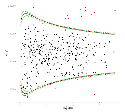
Figure 1: Example of applying the caustics method to the cluster A0085; the caustics are the black solid lines, while the red dashed lines indicate the rms of the fit and the green dashed lines the bootstrap uncertainty (1 000 simulations). Black points (that is, the ones within the caustics) are taken to be the bound members, while red points are discarded as cluster members.

0.3.3 Determination of cluster dynamical parameters

To establish the dynamical properties of each system, we first measure two robust kinematical parameters, known as the biweight central value, $C_{\mathrm{BI}}$, and scale, $S_{\mathrm{BI}}$ (Beers et al., 1990). Using these parameters, we calculate preliminary values for the systemic radial velocities, $v_{\rm c}$, and velocity dispersions, $\sigma_{\rm c}$, considering the $N_{c}$ members. Then we proceed by defining, for each cluster, a projected aperture on the sky consistent with the virial radius.

This implies first estimating $r_{200}$, the radius inside which the mean density of galaxies exceeds $200\times\rho_{c}$ at the redshift of the cluster. Following the prescription by Carlberg et al. (1997):

$$r_{200}=\frac{\sqrt{3}\;\sigma_{\mathrm{c}}}{10\,H(z)}$$ (1)

where $H(z)=H_{0}\sqrt{\Omega_{r}(1+z)^{4}+\Omega_{m}(1+z)^{3}+\Omega_{k}(1+z)^{2}+\Omega_{\Lambda}}$, assuming $\Omega_{r}$ (radiation) and $\Omega_{k}$ (curvature) are about zero. Since the virial radius depends on the redshift and cosmology (e.g., Bryan & Norman, 1998), a local value of $1.3\times r_{200}$, corresponding to about $r_{100}$, is usually adopted (e.g., Kopylova & Kopylov, 2018). Once the circular aperture corresponding to the virial radius is determined, we counted the number of galaxies inside it, $N_{a}$, and recalculated the systemic radial velocity, $v_{\mathrm{cl}}$, and its velocity dispersion, $\sigma_{\mathrm{cl}}$, using once again $C_{\mathrm{BI}}$ and $S_{\mathrm{BI}}$.

These $N_{a}$ galaxies are also used to calculate the projected radius, $R_{\mathrm{p}}$, equal to twice the harmonic mean projected separation, using the relation:

$$R_{\mathrm{p}}={N_{a}(N_{a}-1)}\left(\sum_{i<j}^{N_{a}}\frac{1}{|r_{ij}|}\right)^{-1}$$ (2)

where $r_{ij}$ is the pairwise projected separation between galaxies. Estimation of the virial mass, $M_{\mathrm{vir}}$, follows the relation:

$$M_{\mathrm{vir}}=\frac{\alpha\pi}{2G}\;\sigma_{\mathrm{cl}}^{2}\,R_{\mathrm{p}}$$ (3)

where the factor $\alpha$ quantifies the isotropy level of the system ($\alpha=3$ when complete isotropy is assumed), applied to $\sigma_{\mathrm{cl}}$, while the factor $\pi/2$ is applied to deproject $R_{\mathrm{p}}$ (Limber & Mathews, 1960). Finally, the virial radius is obtained using the relation:

$$R_{\mathrm{vir}}^{3}=\frac{3}{4\pi}\frac{M_{\mathrm{vir}}}{\rho_{\mathrm{vir}}}=\frac{\alpha\;\sigma_{\mathrm{cl}}^{2}\;R_{\mathrm{p}}}{18\pi\,H^{2}(z)}$$ (4)

where the virial density is defined as $\rho_{\mathrm{vir}}=18\pi^{2}(3H^{2}(z)/8\pi G)$.

0.3.4 Substructure analysis

Several tests, in different spatial dimensions, have been proposed for the detection of substructures in galaxy clusters based on optical data: in 1D, as applied to the redshifts (e.g., Bird & Beers et al., 1993; Hou et al., 2009), in 2D, as applied to galaxy projected celestial coordinates (e.g., Geller & Beers, 1982; Fitchett & Webster, 1987; West et al., 1988; Kriessler & Beers, 1997; Flin & Krywult, 2006), and in 3D, as applied to both redshifts and coordinates (e.g., Dressler & Shectman, 1988; Serna & Gerbal, 1996; Pisani, 1996; Einasto et al., 2010; Yu et al., 2015). However, not all these tests have the same efficiency. Through a study of 31 different tests, Pinkney et al. (1996) found the 3D test developed by Dressler & Shectman (1988, DS herafter) to be the most sensitive, concluding that, in general, the higher the dimension of a test, the more powerful it is in distinguishing substructures. This was confirmed subsequently by Einasto et al. (2012), who also showed that 3D tests are more robust than 2D tests, and 2D tests more robust than 1D tests. However, both groups recommended the application of more than one test.

Tests for detecting substructures using X-ray data have also been proposed (e.g., Mohr et al., 1993; Buote & Tsai, 1995; Andrade-Santos et al., 2012). However, because the tests are based on X-ray surface brightness, the detection of substructures is usually limited to the densest, most concentrated ($R<r_{500}$) regions of the clusters (e.g., Piffaretti & Valdarnini, 2008), which might complicate comparisons with substructures detected in the optical. In the study made by Lopes et al. (2018), for example, only $\sim$ 60% of the substructures detected in optical were also detected in X-ray, both inside $r_{500}$. They also found the fraction of substructures to increase with the aperture used, as well as with the mass of the cluster and its redshift (up to $z\sim$ 1; see also Jeltema et al., 2005). Although these trends are consistent with various levels of relaxation (for example, clusters being less relaxed in the past than now), establishing a firm connection as well as a time scale to reconstruct the assembly histories of clusters is not straightforward and needs independent confirmation.

In principle, this is what a study of the CDG dynamical characteristics can contribute. More specifically, the projected position offset of a CDG relative to the X-ray peak and its peculiar velocity relative to the centroid of the distribution of galaxy members are two parameters expected to be correlated with the level of relaxation of the clusters (e.g., Zhang et al., 2011; Lavoie et al., 2016; Lopes et al., 2018): the smaller the offset and peculiar velocity, the higher the level of relaxation. This assumes migration through dynamical friction of the CDG towards the center of the cluster is less rapid than that of the hot gas. Comparing these two parameters with the level of substructuring in clusters –the higher the number of substructures the lower the level of relaxation– should consequently complement our view about their assembly histories.

Thus, to reconstruct the assembly histories of the clusters in our sample, we will develop our study of substructures applying different tests, with different dimensions, in the optical, comparing with X-ray substructuring information and radio data from the literature whenever available, and each time comparing the results (as an independent test) with the dynamical characteristics of the CDGs in their respective clusters.

Radial velocity distributions (1D test):

We start by directly inspecting the LOS velocity distributions of galaxies within the clusters, comparing them with a Gaussian distribution. The physical motivation of this test is the following: as the system tends toward relaxation, the absolute values of skewness and excess kurtosis (with respect to the value of 3 for a Gaussian distribution) also tend to decrease. This is a straightforward test that is easy to quantify.

Adopting a level below 0.3 as an upper limit for relaxation, only 25% of the clusters in our sample present LOS velocity histograms consistent with a Gaussian. This indicates that as much as 75% of the clusters in our sample show a possible signal of being substructured, as disclosed, more specifically, by two or more noticeable peaks in the LOS velocity distribution or platykurtic kurtosis values.

Projected distribution of galaxies (2D-test):

The second test consists in tracing the isodensity contour map of the projected galaxy distribution in each cluster, where any galaxy density peak may be considered as a significant substructure (Geller & Beers, 1982) since only spectroscopically confirmed members were considered. The (probability) density maps were obtained using a bivariate adaptive kernel, fitted by the function:

$$G(x,y)=\frac{1}{2\pi\sigma_{x}\sigma_{y}\sqrt{1-\rho^{2}}}\exp{\left(-\frac{z}{2(1-\rho^{2})}\right)}$$ (5)

where $z$ (do not confuse with redshift) is equal to:

$$z\equiv\frac{(x-\mu_{x})^{2}}{\sigma_{x}^{2}}-\frac{2\rho(y-\mu_{y})(y-\mu_{y})}{\sigma_{x}\sigma_{y}}+\frac{(y-\mu_{y})^{2}}{\sigma_{y}^{2}}$$ (6)

and where, when the parameters $x,y$ are not strongly correlated, one can assume $\rho=0$.

In Fig. 2 the surface density map of the member galaxy distribution of the cluster A0085 is shown as example. In this figure, the isodensity contours are codified in colors, with a cross indicating the density peak. Also shown are the positions of the CDG (open square) and peak in X-ray ($\times$ symbol). Note that although the CDG is slightly off-centered from the distribution of the galaxies, its position is almost the same as the peak in X-ray. Despite the substructures, this looks like a relatively well evolved cluster.

As it is difficult to resume the information on substructure in a table we offer the isodentity maps of all of our clusters on an accompanying web site (www.astro.ugto.mx/recursos/HP_SCls/Top70.html).

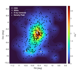
Figure 2: Example of an isodensity map for the cluster A0085. The isodensity levels are coded by colors, in units of the probability density to find spectroscopic member galaxies/deg² (mean probability density equals to 1). The position of the peak in density is indicated, as well as the position of the CDG, SDGs and X-ray centroid.

X-ray surface brightness maps (2D test):

X-ray surface brightness maps are constructed and used as a supplementary information for identifying the substructures. Apart from applying an algorithm to detect independently substructures in these data, we checked every substructure detected in the optical for its counterpart in X-rays. This made possible, for example, to find cases of multimodal main structures that would not be identifiable from the optical data alone.

Using the Aladin interface, we traced the X-ray surface brightness maps for all our clusters, overlaid in red contours on top of the respective DSS2 R-band image. The X-ray data come from ROSAT soft band (surface brightness in the 0.1–2.4 keV). It is worth to note that the all-sky sensitivity of ROSAT is limited to about 10^-13 erg s^-1 cm^-2 (e.g., Vikhlinin et al., 1998; Burenin et al., 2007). This is enough for detecting $k$T${}_{\mathrm{X}}\geq$ 1 keV clusters, but not enough for identifying substructures in the cooler ones. All these maps can also be examined in the webpage accompanying this article.

The example shown in Fig. 3 is once again for A0085. A smoothing parameter of 4 in ds9 was used. The lowest contour in X-ray was traced at the 3$\sigma$ level, followed by contours at levels of 6, 12, 24 and 48 $\sigma$. The cyan $\times$ symbol is the X-ray peak emission, the magenta square locates the CDG and the green circle corresponds to a 0.5 $h_{70}^{-1}$ Mpc radius around it. Usually, an optical image of size 30$\times$30 in the plane of the sky is sufficient to show the distribution of the X-ray emission. Comparing with Fig. 2, one can see that the detected gas in A0085 covers a smaller area (volume) than the distribution of the galaxies in the cluster and that the CDG is only slightly displaced from the X-ray peak.

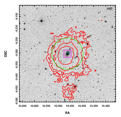
Figure 3: Example of an X-ray map (red contours over the DSS image), for the cluster A0085. The position of the X-ray peak is indicated (cyan ‘$\times$’ symbol), as well as the position of the CDG (magenta square). The green circle marks a 0.5 $h_{70}^{-1}$ Mpc radius around the CDG.

Dressler & Shectman test (3D-test):

The DS-test (Dressler & Shectman, 1988) is performed in two steps. The first step consists in calculating the $\delta_{i}$ parameter for each member galaxy:

$$\delta_{i}^{2}=\frac{N_{nn}+1}{\sigma_{\mathrm{c}}^{2}}[(\bar{v}_{local}-v_{\mathrm{c}})^{2}+(\sigma_{local}-\sigma_{\mathrm{c}})^{2}]$$ (7)

where $v_{\mathrm{c}}$ and $\sigma_{\mathrm{c}}$ are the cluster global parameters, while $\bar{v}_{local}$ and $\sigma_{local}$ are local parameters, calculated for the $N_{nn}=10$ nearest neighbors of each member galaxy (see Bravo-Alfaro et al., 2009, for a discussion of these local parameters and the number of nearest neighbors).

The second step consists in calculating, for each cluster, the parameter $\Delta=\sum\delta_{i}$ and comparing its value with a set of 1000 Monte Carlo simulations, obtaining the probability $p$ that a value $\Delta>\Delta_{observed}$ would have been obtained by chance. We, thus, calculate P${}_{\mathrm{sub}}=100*(1-p)$, which is the probability that the cluster is substructured. Based on this test, a cluster with P${}_{\mathrm{sub}}>$ 90% can be considered to be significantly substructured.

Because $\Delta$ tends to equal the number of galaxy members when the cluster is close to relaxation (e.g., Pinkney et al., 1996), we used the ratio $\Delta/N_{c}$ as an iterative parameter for the test. Note that, different from the traditional way substructures are identified by this test, we do not consider only specific concentrations of galaxies with high $\delta$ values in the projected distribution. Specifically, when $\Delta/N_{c}>$ 1.2, we analyse both the 3D distribution of galaxies in RA, Dec and $v_{local}$ and the respective 2D PPS diagram to identify, in the former, the volume separation surfaces between the substructures (e.g., López-Gutiérrez et al., 2022). In this pseudo-3D volume, substructure members are more smoothly distributed, defining a more isolated locus (local concentration) than in a RA-Dec-$z$-volume, while in the PPS they show the typical caustics-shape distribution. Therefore, after separating the substructures from the remaining main structure, we recalculate $\Delta/N_{c}$ to see whether it is below 1.2, and if not, iterate again to isolate new substructures.

Note that in applying this test there are cases for which it is not correct to assume there is only one main structure. This happens when there are two or more substructures that are comparable in mass, as well as being much more massive than all the other substructures in the cluster. These are examples of “bimodal” or “multi-modal” clusters.

The parameters calculated from the dynamical and substructure analyses are reported in Table 3. In col. 1, we give the updated cluster ID. Note that the entries in Table 3 slightly differ from those in Table LABEL:T_Sample. More specifically, the clusters A2870 and A4049 were determined (see § 0.3.2) to be part of other massive clusters, respectively A2877 and A4038A. On the other hand, two clusters had their well-known LOS components considered separately, A1736 becoming A1736A and A1736B, and A3526 becoming A3526A and A3526B. Consequently, although the number of entries in both tables are the same, 67 clusters, their identities are somewhat different. In Table 3, the equatorial coordinates of the corresponding CDGs (and by convention, cluster centers) are given in cols. 2 and 3, followed in col. 4 by their LOS velocities. Column 5 reports the number of candidate members after splitting up the intersecting neighbors, $N_{g}$, and col. 6, the number of galaxies, $N_{c}$, considered to be bound (included within the caustics) in each cluster. Other dynamical parameters are reported in col. 7 ($v_{\rm c}$), col. 8 ($\sigma_{\rm c}$), both for the $N_{c}$ members, col. 9 ($r_{200}$), col. 10 ($N_{a}$), col. 11 ($v_{\mathrm{cl}}$), col. 12 ($\sigma_{\mathrm{cl}}$), the last three for the members inside the circular aperture, col. 13 ($R_{\rm p}$), col. 14 ($R_{\mathrm{vir}}$) and col. 15 ($M_{\mathrm{vir}}$). Parameters associated to the substructure analyses are shown in columns 16 to 18: the skewness, the excess kurtosis, and P${}_{\mathrm{sub}}=100*(1-p)$, respectively.

Note that some clusters in our sample do not have their ICM emission centered on the main structure of their clusters, but on a substructure (A0754, A1736B and A2151). These are marked with a ’${}^{\cancel{x}}$’ in the first column of the Table 3.

0.3.5 Gravitational binding

For the 16 superposed clusters appearing in Table 2, as well as for the substructures reported in Table LABEL:T_ApB, we complemented our analysis by applying a test for gravitational binding. Since the evolutionary state of a system like a galaxy cluster is also related to its geometry in redshift space, any density enhancement present in real space will also appear as a density enhancement in redshift space: systems representing small overdensities, where the Hubble flow has not yet been significantly perturbed, appear essentially undistorted, while those that are clearly collapsing, the Hubble flow being slowed down, appear flattened along the LOS. On the other hand, systems that are close to virial equilibrium appear as particularly elongated condensations in redshift space, a phenomenon known in the literature as Fingers-of-God. Because of this effect, it is therefore possible to assess what is the global dynamical state of a galaxy system at the scale of a cluster by evaluating its distortions in redshift space.

As explained by Sargent & Turner (1977), this level of distortion can be determined, for a pair of objects (galaxies, groups or clusters), by determining the separation between the members of the pair and the angle $\chi$ between the separation vector and the plane of the sky. Such angle is measured as follows: let $\theta_{12}$ be the angular separation between the center of the two galaxies, $z_{1}$ and $z_{2}$ (with $z_{2}\geq z_{1}$) being their respective redshifts, then the physical distance ($d_{12}$) and projected separation ($\ell_{12}$) in the plane of the sky are given, respectively, by:

$$d_{12}=\frac{c}{H_{0}}\left[z_{1}^{2}+z_{2}^{2}-2z_{1}z_{2}\cos{\theta_{12}}\right]^{1/2}$$ (8)

and

$$\ell_{12}=\frac{c}{H_{0}}\left(z_{1}+z_{2}\right)\tan{\frac{\theta_{12}}{2}}$$ (9)

the angle $\chi$ between the separation vector being equal to:

$$\chi=\arctan\left[\frac{1}{2}\left(\frac{z_{2}}{z_{1}}-1\right)\cot{\frac{\theta_{12}}{2}}\right]$$ (10)

where $0\leq\chi\leq\pi/2$.

For a homogeneous spherical system following the expansion flow, $\langle\chi\rangle$ approaches the isotropic value of 32.7^∘; $\langle\chi\rangle$ tends to lower values for a collapsing (flattened) system and larger values for a virialized (elongated) one. Note, however, that for a non-spherical system, the geometrical elongation/flattening could dominate $\langle\chi\rangle$, masking their real dynamical state.

22

Table 3: Basic data on clusters of the sample.

IDa	RACDG	DecCDG	$v_{\mathrm{CDG}}$	$N_{g}$	$N_{c}$	$v_{c}$	$\sigma_{c}$	$r_{200}$	$N_{a}$	$v_{\mathrm{cl}}$	$\sigma_{\mathrm{cl}}$	$R_{\mathrm{p}}$	$R_{\mathrm{vir}}$	$M_{\mathrm{vir}}$	skew	kurt	Psub	$N_{\mathrm{sub}}$	$\cal{A}$	$r_{\mathrm{ox}}$	$v_{\mathrm{pec}}$
	[deg]J2000	[deg]J2000	[km/s]			[km/s]	[km/s]	[Mpc]b		[km/s]	[km/s]	[Mpc]b	[Mpc]b	[$M_{\odot}$]b			[%]	m,hs,ls		[kpc]b	[km/s]
(1)	(2)	(3)	(4)	(5)	(6)	(7)	(8)	(9)	(10)	(11)	(12)	(13)	(14)	(15)	(16)	(17)	(18)	(19)	(20)	(21)	(22)
A2798B	9.37734	-28.52947	33338	81	78	33604	697	1.353	60	33544	757	1.148	1.748	6.01	-0.313	-0.502	87.4	1,0,0	U	96.5	-185.3
A2801	9.62876	-29.08160	33660	50	45	33773	652	1.259	35	33640	699	1.553	1.833	6.94	-0.397	-0.024	15.5	1,0,0	U	42.4	18.0
A2804	9.90753	-28.90620	33546	88	80	33378	663	1.292	48	33669	516	1.277	1.403	3.11	-0.346	-0.982	97.6	2,0,0	M	126.3	-110.6
A0085A	10.46051	-9.30304	16613	368	352	16561	1011	2.027	321	16570	1045	2.030	2.668	20.20	-0.444	-0.118	99.9	1,2,3	S	8.2	32.2
A2811B	10.53717	-28.53577	32466	146	139	32354	831	1.625	103	32329	947	1.701	2.316	13.90	0.162	-0.042	94.3	1,0,2	S	5.5	123.7
A0118	13.74348	-26.37515	34068	119	80	34384	681	1.341	59	34287	689	1.206	1.667	5.23	0.349	-0.635	90.4	1,2,0	S		-212.7
A0119	14.06709	-1.25549	13323	339	333	13299	810	1.633	294	13301	853	1.430	2.082	9.51	-0.175	0.246	99.9	1,2,1	S	125.2	21.1
A0122	14.34534	-26.28134	33804	111	31	34076	659	1.265	28	34062	677	1.190	1.641	4.98	0.337	-0.266	46.8	1,0,0	U	50.6	-231.7
A0133A	15.67405	-21.88215	17048	137	132	16830	713	1.425	86	16838	778	1.320	1.899	7.30	0.077	-0.393	77.7	1,2,0	S	33.9	198.8
A2877-70	17.48166	-45.93122	7213	237	174	7034	652	1.326	112	7143	679	0.999	1.596	4.20	0.273	-0.398	100.0	1,2,0	S	27.8	68.4
A3027A	37.70600	-33.10375	23541	167	102	23429	668	1.335	82	23494	713	1.618	1.904	7.52	-0.278	-0.814	97.2	1,1,1	S	113.9	43.6
A0400	44.42316	6.02700	6789	115	61	6959	323	0.682	51	6947	343	0.635	0.870	0.68	0.100	-1.007	76.0	1,1,0	S	39.8	-154.4
A0399	44.47119	13.03080	21483	101	69	21138	957	1.894	69	21146	950	1.414	2.209	11.70	-0.225	-0.460	13.3	1,0,0	U	110.1	314.8
A0401	44.74091	13.58287	22297	116	115	22053	1028	2.036	114	22061	1026	1.574	2.407	15.10	0.263	-0.352	40.8	1,0,0	U	18.6	219.8
A3094A	47.85423	-26.93122	20552	126	114	20489	548	1.090	84	20539	637	1.305	1.648	4.83	0.628	0.243	88.3	1,0,0	U	148.3	12.2
A3095	48.11077	-27.14016	19314	44	40	19485	306	0.606	21	19557	327	0.664	0.845	0.65	-0.018	-0.932	10.5	1,0,0	L		-228.1
A3104	48.59055	-45.42024	21785	62	53	21777	413	0.823	28	21681	498	0.782	1.178	1.77	0.039	-0.106	39.5	1,2,0	S	34.4	97.0
S0334	49.08556	-45.12110	22401	22	27	22373	518	1.030	26	22363	534	0.811	1.249	2.11	0.449	1.037	27.4	1,0,0	L		35.4
A3112B	49.49025	-44.23821	22764	120	97	22631	672	1.337	74	22669	705	1.861	1.982	8.46	0.271	-0.572	99.9	1,1,0	S	13.2	88.3
S0336	49.45997	-44.80069	22849	54	44	23223	506	1.006	32	23186	538	1.140	1.405	3.02	0.178	-0.606	3.2	1,0,0	L		-312.8
A0426A	49.95042	41.51167	5231	360	314	5254	1030	2.104	314	5262	1029	1.395	2.359	13.50	0.030	-0.535	97.1	1,0,2	P	4.0	-30.5
S0373	54.62118	-35.45074	1452	272	229	1452	334	0.688	98	1461	390	0.308	0.749	0.430	-0.025	-0.428	100.0	1,2,1	S	1.7	-9.0
A3158	55.72063	-53.63130	17327	258	249	17764	1064	2.138	249	17735	1066	1.341	2.353	13.90	0.260	-0.478	49.6	1,2,2	S	19.1	-385.2
A0496	68.40767	-13.26196	9841	358	351	9892	688	1.395	279	9925	712	1.364	1.822	6.31	0.030	-0.535	99.9	1,1,0	S	8.5	-81.3
A0539	79.15555	6.44092	8257	143	132	8679	571	1.160	92	8631	698	0.882	1.557	3.92	-0.249	0.825	100.0	1,2,0	S	6.5	-363.5
A3391	96.58521	-53.69330	16361	119	100	16831	760	1.519	75	16776	817	1.270	1.936	7.74	0.159	-0.482	9.8	1,0,0	U	24.4	-393.0
A3395	96.90105	-54.44936	14571	224	218	14875	722	1.450	199	14878	746	1.264	1.823	6.42	-0.158	-0.494	100.0	2,2,1	M	10.9	-292.5
A0576	110.37600	55.76158	11435	238	220	11351	810	1.638	191	11350	866	1.633	2.202	11.20	0.031	-0.114	100.0	1,2,0	S	84.3	81.9
A0634	123.93686	58.32109	8029	140	132	8006	318	0.646	70	8037	395	0.792	1.029	1.13	0.057	-0.061	73.4	1,0,0	L		-7.8
A0754${}^{\cancel{x}}$	137.13495	-9.62974	16451	468	386	16246	757	1.520	333	16258	820	1.484	2.045	9.10	-0.024	0.373	100.0	2,2,2	M	239.1	183.1
A1060	159.17796	-27.52858	3808	382	380	3709	652	1.335	343	3694	678	0.951	1.574	3.99	0.122	-0.532	100.0	1,0,5	P	4.9	112.6
A1367	176.00905	19.94982	6260	339	286	6451	547	1.115	226	6444	597	1.157	1.539	3.76	-0.026	-0.629	100.0	2,0,2	M	366.0	-180.1
A3526A	192.20392	-41.31166	2948	235	235	3088	491	1.005	126	2993	564	0.836	1.335	2.43	-0.482	-0.191	100.0	1,0,3	P	3.8	-44.6
A3526B	192.51645	-41.38207	4593	101	95	4580	276	0.552	45	4636	317	0.480	0.754	0.44	0.300	-0.359	99.9	1,1,0	S		-42.3
A3530	193.90001	-30.34749	16187	126	110	16036	615	1.231	94	16064	631	1.272	1.632	4.63	0.305	-0.567	99.5	1,1,0	S	66.5	116.7
A1644	194.29825	-17.40957	14225	307	301	14085	987	1.989	288	14095	1008	1.507	2.365	14.00	-0.049	0.201	86.6	1,0,2	P	39.6	124.2
A3532	194.34134	-30.36348	16303	112	103	16753	423	0.849	58	16709	443	0.929	1.160	1.66	-0.130	-0.798	93.5	1,2,0	S	87.9	-384.6
A1650	194.67290	-1.76139	25328	220	192	25216	673	1.330	146	25249	723	1.581	1.903	7.55	0.188	0.016	2.1	1,0,0	U	27.3	72.9
A1651	194.84383	-4.19612	25622	221	191	25454	833	1.651	158	25453	876	1.782	2.250	12.50	0.132	-0.569	59.2	1,0,2	P	25.5	155.8
A1656	194.89879	27.95939	7157	969	969	6976	993	2.025	919	6997	995	1.734	2.474	15.70	-0.100	-0.018	100.0	1,1,8	S	57.9	156.4
A3556	201.02789	-31.66996	14406	102	102	14435	505	1.016	90	14436	520	1.048	1.347	2.59	0.354	-0.606	99.0	2,0,0	M	630.5	-28.6
A1736A	201.68378	-27.43940	10506	74	74	10363	417	0.840	36	10499	386	0.955	1.075	1.30	0.102	-0.997	100.0	1,3,0	S		6.8
A1736B${}^{\cancel{x}}$	201.86685	-27.32468	13574	145	141	13665	839	1.689	126	13678	844	1.355	2.029	8.82	0.022	-0.500	99.0	1,1,1	S	610.8	-99.5
A3558	201.98701	-31.49547	14073	548	548	14455	950	1.912	469	14476	955	1.893	2.460	15.80	-0.230	-0.478	100.0	1,0,1	P	25.0	-384.4
A3562	203.39474	-31.67227	14693	231	98	14541	564	1.138	82	14561	594	1.221	1.549	3.94	0.037	-0.634	43.6	1,0,0	U	42.6	125.9
A1795	207.21880	26.59301	18968	179	164	18893	764	1.525	154	18889	780	1.278	1.876	7.09	-0.049	0.210	98.3	1,0,0	U	13.8	74.3
A2029	227.73376	5.74491	23353	202	155	23052	934	1.850	155	23051	931	0.989	1.931	7.82	0.096	-0.791	92.8	1,0,0	U	132.8	280.4
A2040B	228.19781	7.43426	13713	153	150	13472	567	1.141	104	13527	627	1.327	1.653	4.77	0.312	0.026	97.8	1,1,0	S	43.3	178.0
A2052	229.18536	7.02167	10332	178	176	10295	581	1.179	120	10416	648	1.115	1.600	4.28	0.356	0.003	100.0	1,1,0	S	9.1	-81.2
A2065	230.62053	27.71228	21828	204	169	21889	1043	2.071	168	21878	1043	1.712	2.504	17.00	0.129	-0.720	99.0	1,0,0	U	47.1	-46.6
A2063A	230.77209	8.60918	10377	200	193	10312	667	1.350	142	10345	762	1.165	1.809	6.18	-0.069	-0.132	99.4	1,0,1	P	16.5	30.9
A2142	239.58345	27.23335	27254	232	191	26975	820	1.618	157	27036	828	1.767	2.157	11.10	-0.087	-0.276	66.7	1,0,1	P	41.0	200.0
A2147	240.57086	15.97451	10595	481	453	10929	918	1.858	397	10889	935	1.966	2.466	15.70	0.215	-0.286	100.0	2,2,0	M	119.9	-283.7
A2151${}^{\cancel{x}}$	241.28754	17.72997	9378	331	311	10906	743	1.502	276	10898	768	1.551	1.999	8.35	-0.064	-0.573	100.0	3,2,2	M	3.1	-1466.6
A2152	241.37175	16.43579	13268	124	116	13283	398	0.799	64	13266	406	1.038	1.139	1.56	0.934	0.724	98.6	2,0,0	M	42.1	1.9
A2197	246.92114	40.92690	9511	294	276	9108	546	1.109	185	9114	573	1.402	1.593	4.21	0.258	-0.797	100.0	3,0,1	M	16.9	385.3
A2199	247.15948	39.55138	9296	521	498	9089	753	1.529	459	9090	779	1.302	1.907	7.21	-0.055	-0.058	100.0	1,0,3	P	6.4	199.9
A2204A	248.19540	5.57583	45528	111	96	45274	760	1.456	38	45497	1101	1.838	2.588	20.30	0.669	0.092	95.5	1,2,0	S	52.1	26.9
A2244	255.67697	34.06010	29543	106	102	29811	1154	2.282	102	29778	1161	1.491	2.546	18.30	0.166	-0.851	63.8	1,0,0	U	15.2	-213.8
A2256	256.11352	78.64056	17778	295	280	17567	1222	2.449	280	17567	1222	1.514	2.683	20.60	0.009	-0.624	99.9	1,2,2	S	129.2	199.3
A2255	258.11981	64.06070	22068	189	181	24100	992	1.973	179	24126	1000	1.802	2.470	16.40	-0.316	-0.518	100.0	1,2,0	S	183.7	-1904.7
A3716	312.98715	-52.62983	14112	157	140	13517	746	1.501	123	13508	783	1.247	1.878	6.99	0.168	-0.915	88.8	2,0,1	M	0.9	578.0
S0906	313.18576	-52.02746	13947	62	54	14481	340	0.680	26	14446	440	0.824	1.113	1.46	0.002	0.014	57.4	1,0,0	L		-476.1
A4012A	352.96231	-34.05553	16241	93	85	16219	473	0.947	39	16249	575	1.043	1.436	3.15	-0.126	0.431	73.1	1,0,0	L		-7.6
A2634	354.62244	27.03130	9117	192	185	9262	695	1.409	166	9268	717	1.251	1.780	5.87	-0.274	-0.177	94.9	1,1,0	S	51.7	-146.5
A4038A-49	356.93768	-28.14070	8672	247	237	8799	683	1.385	180	8873	753	1.150	1.789	5.95	0.252	-0.017	100.0	1,2,0	S	14.4	-195.2
A2670	358.55713	-10.41900	23157	308	288	22791	909	1.805	251	22799	970	1.153	2.089	9.91	0.066	-0.258	100.0	1,0,0	U	31.7	332.7
aA capital letter after the ACO name indicates the line-of-sight component of the cluster (see Chow-Martínez et al., 2014). A ${}^{\cancel{x}}$ symbol indicates the cluster center is not at the X-peak substructure. bLongitud and mass parameters are also in units of $h_{70}$.

Assuming a symmetric geometry, on the other hand, the same angle $\chi$ can be used to test the Newtonian criterion for gravitational binding of two systems (Beers et al., 1982). This allows one to determine whether the pairs are either relaxed, collapsing or expanding, or not bound but simply close in space. Within the context of a two-body-problem, the orbits of the two galaxies or systems, with masses $M_{1}$ and $M_{2}$, are assumed to be linear, with no rotations or discontinuities around the center of mass. The projected separation between their centers would then be $R_{p}=R\cos{\chi}\,(=\ell_{12})$ and their relative velocity projected along LOS, $V_{r}=V\sin{\chi}$, where $R$ is the physical distance ($=d_{12}$) between them and $V$ is their relative velocity. Considering that the energy criterion for gravitational binding is, $\frac{1}{2}v_{esc}^{2}\leq\frac{GM}{R}$, where $v_{esc}$ is the escape velocity, we assume $V=v_{esc}$ and estimate the total mass to be $M=M_{1}+M_{2}$, yielding the condition for the pair to be bound:

$$V_{r}^{2}R_{p}\leq 2GM\sin^{2}{\chi}\cos{\chi}$$ (11)

Having evaluated these parameters for the 16 cases of superposed clusters in our sample, this is how we determined, as reported in Table 2, that 5 pairs and 2 clusters are only apparent superpositions.

0.3.6 CDG related parameters

CDG–X-ray offset:

The offsets for 52 of the 59 clusters detected in X-rays in our sample were calculated based on the coordinates of the peak emission in X-ray compiled by Piffaretti et al. (2011). However, for A2151 we did not use this source because the peak reported by these authors, although the brightest in this cluster, corresponds to the emission of a subcluster. Instead, we used the coordinates of the main structure as reported by Tiwari & Singh (2021). For 5 of the 6 remaining clusters, the coordinates for the X-ray peaks came from three different studies (Ebeling et al., 1996; Ledlow et al., 2003; Sato et al., 2010). This leaves one cluster, namely A0118, for which information is missing. The offsets, $r_{\mathrm{ox}}$, reported in col. 21 of Table 3, correspond to the angular separations transformed into the physical separations in kpc at the redshift of each cluster.

To compare these offsets with those reported in the literature, we also calculated the relative offsets, using the relation:

$$\Delta r_{\mathrm{ox}}=r_{\mathrm{ox}}/r_{500}$$ (12)

Note that since Piffaretti et al. (2011) is our only source for $r_{500}$, we only calculated $\Delta r_{\mathrm{ox}}$ for the 52 clusters in common with these authors (to be reported further in Table LABEL:T_Assembl).

Consistent with a typical cooling time of 4 Gyr (see Figure 2 in Zhang et al., 2011), a cluster with an offset $r_{\mathrm{ox}}<30\ h_{70}^{-1}$ kpc, equivalent to $\Delta r_{\mathrm{ox}}\lesssim 0.03$, can be considered to be relaxed. Compared with the literature, this relaxation threshold is between two previously proposed values: Lavoie et al. (2016) used $\Delta r_{\mathrm{ox}}=0.05$ and Lopes et al. (2018) used $\Delta r_{\mathrm{ox}}=0.01$.

Peculiar velocity:

We calculated the peculiar velocity of the CDGs using the formula (e.g., Coziol et al., 2009):

$$v_{\mathrm{pec}}=\frac{v_{\mathrm{CDG}}-v_{\mathrm{cl}}}{1+z_{\mathrm{cl}}}$$ (13)

We also calculated the respective relative peculiar velocity using the definition (e.g., Lauer et al., 2014):

$$\Delta v_{\mathrm{pec}}=|v_{\mathrm{pec}}|/\sigma_{\mathrm{cl}}$$ (14)

We report the values obtained for $v_{\mathrm{pec}}$ in col. 22 of Table 3, while $\Delta v_{\mathrm{pec}}$ will be reported in Table LABEL:T_Assembl. According to this parameter, we consider a system to be relaxed when $|v_{\mathrm{pec}}|<175$ km s^-1, which is equivalent to $\Delta v_{\mathrm{pec}}\lesssim 0.21$.

CDG luminosities:

As described in § 0.2.3, we used the K_s absolute magnitudes of the CDGs, M_Ks, as a proxy for their stellar masses. Comparison of these masses with the masses (or number of galaxies) of the substructure hosting the CDGs can yield important information about the assembly histories of the clusters. In particular, one could expect the most massive CDGs to be located in the most massive substructures, and these massive substructures to form the main subclusters of their respective clusters. The absolute magnitudes of the CDGs are reported further in Table LABEL:T_Assembl.

Magnitude gaps:

Another important parameter relating the assembly history of the CDG to its cluster is its magnitude gap: assuming a CDG grows in mass by cannibalizing its neighbors, its magnitude gap is expected to increase with time. For our sample, we have calculated two gaps: i) the difference in magnitude between the CDG and second-rank member, $\Delta m_{12}$, and ii) the difference in magnitude between the second and third-rank members, $\Delta m_{23}$.

Note that when a CDG differs from the original BCG of the cluster (which is the case for 19% of the clusters in our sample, see § 0.3.1), the identification of the second-rank galaxy varies with the type of cluster: for both the Fornax-like clusters and clusters with a fossil candidate in their outskirts, the second-rank galaxy is the second-rank of the main structure, while in Coma-like cluster the second-rank is the initial BCG, brighter than the CDG; this produces a negative $\Delta m_{12}$. The various gaps are also reported in Table LABEL:T_Assembl.

0.4 Properties and assembly histories of clusters

0.4.1 Global cluster properties

Using the optical data related to galaxy membership, we show in Fig. 4 the histograms characterizing the “global” properties of the clusters identified in Table 3. In the upper left panel, we show the distribution of $r_{200}$, which is commonly used as a reference radius. The median of 1.35 $h_{70}^{-1}$ Mpc, corresponding to only 63% of the R_A, implies the galaxy concentrations in our sample of clusters are relatively high. In the upper right panel, the two distributions for the number of galaxies within the caustic, $N_{c}$, and galaxies within virial aperture radius, $N_{a}$, confirm this trend, the medians amounting to 150 and 114 galaxies, respectively. In the lower left panel, the distribution of redshifts is found to be positively skewed, since the mode appears before the median at $z=0.054$. This shows that most of our clusters are nearby, and thus, assuming they formed in the distant past, had had enough time to virialize. Finally, in the lower right panel, the distribution for the velocity dispersion within $1.3\times r_{200}$ has a median value of 723 km s^-1, which is typical for Abell clusters.

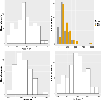
Figure 4: Global properties of the clusters as defined in Table 3: Upper left, estimated $r_{200}$ radii; upper right, number of galaxies within the caustics ($N_{c}$, orange) and within the virial radius ($N_{a}$, gray); lower left, redshifts; and lower right, velocity dispersions ($\sigma_{cl}$).

Based on the above distributions, we conclude that our sample is composed mostly of nearby, relatively rich clusters, where the concentrations of galaxy and velocity dispersion are remarkably high, justifying the assumption that those are systems that had had sufficient time to evolve internally and should then be expected to be close to virialization. Consistent with this assumption, the distribution of the virial masses in the right panel of Fig. 5 is found to be significantly negatively skewed, with a median 6.4 $\times 10^{14}$ $h_{70}^{-1}$ $M_{\odot}$. However, the distribution for the virial radii, in the left panel, does not follow this trend, spannig a relatively large range, with a median value of 1.82 $h_{70}^{-1}$ Mpc, corresponding to 0.85 times the R_A. This peculiarity may suggest that the clusters either have different assembly states or even different assembly histories.

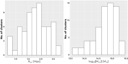
Figure 5: Distributions of virial radius (left panel) and virial mass (right panel).

Comparing our virial masses with those of the literature was not straightforward, since published estimates of these are rare. One suitable source is the GalWeight cluster catalog (GalWCat19; Abdullah et al., 2020), where the masses of 1 800 clusters were determined within three different projected radii: $r_{100}$, $r_{200}$ and $r_{500}$. There are 18 clusters in this catalog that are also in our sample, and we compare, in Fig. 6, their three different masses, $M_{100}$, $M_{200}$ and $M_{500}$ with our $M_{\mathrm{vir}}$ estimate. The three linear fits we obtained are relatively good, with comparable correlation coefficients R $\sim$ 0.83, 0.87 and 0.89, respectively. However, since our virial masses were estimated using a proxy for $r_{100}$ (cf. § 0.3.3), the comparison that counts for us is with $M_{100}$. In the lower panel, the fit shows our virial mass estimate to be in good agreement with those of GalWCat19 for $r_{100}$, the residuals being due probably to the different ways the membership of galaxies in each cluster was determined, and the mean redshifts of galaxies in our data compared to only SDSS redshifts in theirs.

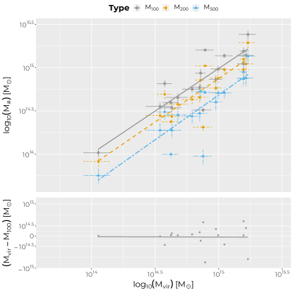
Figure 6: Comparison of our mass estimates with the virial masses in the GalWeight galaxy cluster catalog. Blue triangles, $M_{500}$, orange circles, $M_{200}$ and gray squares $M_{100}$. The three lines are linear fits to points with the same colors. In the lower panel, the residual corresponds to the comparison of our virial mass with $M_{100}$.

To disentangle the assembly history of these clusters, we discuss in the following sections the implications of various dynamical parameters and classifications obtained for three different internal regions within the clusters. The three regions are the following: i) the outer region, from $R_{\mathrm{vir}}$ down to $r_{500}$, as traced by the optical data on galaxy membership; ii) the inner region, inside $r_{500}$, as traced by X-ray emission; iii) and the innermost core, characterized by gas cooling and CDG properties. Typical radii for these regions are $R_{\mathrm{vir}}\sim 1.8\,h_{70}^{-1}$ Mpc, $r_{500}\sim 0.9\,h_{70}^{-1}$ Mpc and core radius ($r_{core}$) about 0.3 $h_{70}^{-1}$ Mpc (note that more specific values will be defined for the various radii as our analysis progresses).

0.4.2 Outer region

The assembly state of the outer region is characterized by the presence or absence of substructures (cf. § 0.3.4). According to the DS-test, the 43 clusters with P${}_{\mathrm{sub}}\geq$ 90% in col. 18 of Table 3 could be considered to have substructures. This represents 64% of our cluster sample. However, considering all the results for the different tests, substructures appear to be secure in only 39 of these clusters and probable, with P${}_{\mathrm{sub}}\lesssim$ 90%, in 8 further clusters. In total, the number of clusters with substructures in our sample could thus be as high as 70%. Consequently, since either fraction is relatively high, it seems safe to conclude that substructures are extremely common in nearby clusters.

Taken at face value, the presence of numerous clusters with substructures suggests that many of these systems did not yet reach equilibrium, and what we observe, consequently, are different phases of a still ongoing process. To better characterize these different phases, it seems therefore important to first classify all the substructures in terms of their dynamical significance. This implies determining the gravitational impact that a substructure, when present, has on the whole cluster.

As a first approximation, this gravitational impact can be estimated by comparing the relative richness, $N_{s}/N_{c}$, formed by the ratio of the number of galaxies in each substructure, $N_{s}$, to the total number of galaxies within the caustics, $N_{c}$. Using the numbers in Table LABEL:T_ApB of Appendix 0.7, we distinguish three levels of dynamical significance:

Main (m):

High relative richness, $N_{s}/N_{c}\geq 0.50$. This level characterizes the dynamically dominant substructures in any cluster. In the case of multi-modal clusters (for example, A2804), the sum of the membership ratios of the main modes is indeed larger than 0.50. In Table LABEL:T_ApB, the substructures with this level of significance are identified by appending the suffix m to their ID.

Highly significant (hs):

Intermediate relative richness, $0.05\leq N_{s}/N_{c}<0.50$. This level characterises substructures that are sufficiently massive to affect the dynamics of their host clusters. In Table LABEL:T_ApB the suffixes (n, s, e, w, c, or a combination thereof) are added to the ID of the substructures indicating its location relative to the main structure (North, South, East, West or central, respectively).

Low-significance (ls):

Low relative richness, $N_{s}/N_{c}<0.05$. These are low-mass clumps of galaxies, attached to a more massive host cluster, that do not affect its dynamics. They are not listed in Table LABEL:T_ApB.

It is worth to note that the m substructure in our sample with the lowest value of $N_{s}/N_{c}$ is A1736Am (0.581), while the hs substructure with the highest $N_{s}/N_{c}$ is A3027Acw (0.235). Thus, the cut in $N_{s}/N_{c}=0.5$ seems to be a good discriminator for this separation. The numbers of substructures with relative richness levels m, hs and ls are indicated in col. 19 of Table 3 using three numbers (m, hs, ls). For example, while A2798B and A2801 only have one main structure each, $N_{\mathrm{sub}}=(1,0,0)$, A2804, a bimodal cluster, has two, $N_{\mathrm{sub}}=(2,0,0)$. A more complex cluster is A0085A, which has one main structure, two hs and three ls substructures, $N_{\mathrm{sub}}=(1,2,3)$. A still more complex cluster is A2151, a trimodal cluster marked as $N_{\mathrm{sub}}=(3,2,2)$.

In col. 20 of Table 3 an extra parameter appears, $\cal{A}$, which is used to qualify the “assembly state” of a cluster based on its level of substructuring. This classification was inspired by the morphological classifications of ICM X-ray emission proposed in Buote & Tsai (1995) and Jones & Forman (1999). We distinguish five assembly states: high-mass, Unimodal clusters (U); Low-mass unimodal (L); Multi-modal (M); Primary (P) with only ls substructures attached to the m mode; and finally Substructured (S), formed by the m mode and at least one hs substructure.

The way we distinguish between U and L clusters depends on the mass criterion $3.5\times 10^{14}M_{\odot}$: U is more massive and L less massive or equal to this mass. In fact, the regular (unimodal) clusters may be either the “beginning” or the “end” of a merging process. They are the beginning if the poor clusters have had time to arrive close to relaxation, while in a relatively isolated environment. As the end, they are the final result of the virialization process of rich clusters. In fact there is no theoretical criterion justifying this distinction, and we chose pragmatically a threshold: the clusters for which we could see relatively relaxed X-ray isophotes were assumed to be close to virialization, while, in the abscence of X-ray emission (implying a less dense or colder ICM, undetectable with ROSAT sensitivity, for example), we assumed the other state.

To be classified as M, a cluster must be formed by two or more m modes, with comparable richness. Consequently, in M clusters the CDG of the cluster is ill-defined, since there are different SDGs competing for this position (one for each mode, at least). For practicality, we choose as the CDG the SDG of the most central mode (usually the richest in galaxies and/or brightest in X-ray). This convention allows us to define a central position for the cluster and serves as reference for the magnitude gaps. Of the ten M-type clusters identified in Table 3, three, namely A0754, A2147 and A2152, show multiplicity only in the optical, while four, A1367, A2151, A2197 and A2804, show multiplicity in both optical and X-rays, and three others, A3356, A3395 and A3716, only in X-rays.

Finally, S and P clusters have both only one main structure and some substructures: in an S cluster there are hs substructures and in a P cluster they are all ls.

Adopting the above definitions, we count 21% U, 13% P, 42% S, 15% M and 9% L clusters. In terms of masses, Table 4 shows that U and P clusters are more massive than S and M clusters, while L clusters are the least massive of all. Thus, poor L clumps could represent the building blocks of future ’massive’ clusters. Also, the distribution in radii presented in Table 4 reveals that the “size” of a cluster and, most specifically, its virial radius increases with its mass.

7 Cluster N $M_{\mathrm{vir}}$ $R_{\mathrm{vir}}$ $r_{200}$ $r_{500}$ $r_{core}$ class mean(median) mean(median) mean(median) mean(median) mean(median) [$10^{14}M_{\odot}$] [Mpc] [Mpc] [Mpc] [Mpc] U 14 9.2(7.7) 1.99(1.93) 1.60(1.52) 0.94(1.05) 0.32(0.31) P 9 9.6(11.1) 2.02(2.16) 1.61(1.62) 1.04(1.00) 0.32(0.34) S 28 8.1(6.3) 1.81(1.82) 1.38(1.39) 0.79(0.92) 0.29(0.29) M 10 6.2(6.4) 1.72(1.82) 1.32(1.45) 0.56(0.63) 0.27(0.29) L 6 1.9(2.1) 1.18(1.25) 0.82(0.95) - (-) 0.19(0.20)

Table 4: Typical parameters in different assembly class clusters

Although 70% of the clusters (M, S and P) show some evidence of substructuring, considering the significance in terms of relative richness and mass, only 57% (M and S) are expected to be dynamically affected by their substructures. This implies that at least 57% of the clusters in our sample have not yet reached virialization. This may be compared to previous numbers reported for local cluster samples, e.g. Lopes et al. (2018), who found that substructuring ranges between 37–75%, in 40 SZ-detected clusters, and between 32–65%, in 62 X-ray clusters (both samples taken from Andrade-Santos et al., 2017). As a whole, for 31 clusters in common with these authors, our results agree for 80% of them.

How does this classification of substructures fit the model of cluster formation? According to the hierarchical model, clusters form mainly by the mergers of groups of galaxies. Within this paradigm U-type clusters would be examples of systems that merged in the distant past and their virialization process would thus be well advanced. P-type clusters would also have formed in the past and represent cases that, being massive, have recently attracted small groups in their environment without an important change in their relaxation state. This reinforces the idea that the cluster formation process is continuous. Consequently, clusters with significant substructures (M and S) would be examples of relatively more recent mergers (which occurred in the last 1–2 Gyr; Lisker et al., 2018; Benavides et al., 2020; Haggar et al., 2023). Their differences are explained by the importance of the merger: in S-type clusters a massive clump is accreting smaller mass groups (minor mergers), while in M-type clusters the masses of the merging entities are comparable (major mergers). Since average masses of M-type clusters are smaller, they could represent the previous step of the formation of the massive main clumps of S-type clusters. By comparing the sum of the merging masses (main + substructures) with the total mass of the cluster, in S clusters the merging masses are 7% less massive than the cluster mass (median 10%), compared to 23% (median 30%) in M clusters. Obviously, M clusters must be relatively less relaxed than the S clusters.

The best examples of poor clusters might be the six L clusters. Indeed, the relatively low masses and small numbers of member galaxies in these systems make them comparable to groups. This might also explain why these poor clusters are not observed in X-ray: simply because they do not have sufficiently deep potential wells for infalling gas to heat up and emit detectable amounts of X-rays. This is the case of candidate AXU clusters like A0634 and A4012, for which confirmation should be obtained using eROSITA (Predehl et al., 2021). The four remaining L clusters also look like they could be either infalling or satellite groups of more massive clusters (see Table 2): these are the cases of S0334 related to A3104, S0336 related to A3112B, and possibly A3095 related to A3094A and S0906 related to A3716 (for which binding could not be established). Other infalling groups, composed by two clumps either and residing well inside the caustics of their main cluster are: A2870, related to A2877, and A4049, related to A4038. These cases would also be excellent candidates to search for evidence, in their galaxies’ properties, of pre-processing.

0.4.3 Inner region

The region inside $r_{500}$ is where the gas accumulates and gets very hot, emitting in X-rays. In our sample, only eight clusters are undetected in X-rays (Table LABEL:T_Sample). However, quantitative information on ICM evolution is scarce and restricted to two parameters: dynamical status of the cluster ICM (71% of X-ray detected clusters) and core cooling status (81%). In Table LABEL:T_Assembl the values for these parameters in clusters with different $\cal{A}$ classes are reported in cols. 2 and 4, respectively. In col. 2, the symbol ✓ indicates a relaxed status while an $\ast$ indicates a disturbed ICM. The main sources for this information were Parekh et al. (2015) and Laganá et al. (2019). In general, conclusions about the dynamical state of the inner region are confirmed by the different sources, except in four cases, the clusters A2029, A2052, A2063A and A2244, for which evidence of disturbance is still debated. In col. 3 of Table LABEL:T_Assembl we added information about the detected presence of radio halos and/or radio relics, mostly from Van Weeren et al. (2019), Knowles et al. (2022) and Botteon et al. (2022). For the 4 cases above, these data indicate disturbance for A2029, A2063A and A2244, and no information concerning diffuse radio emission for A2052. In general, the presence of radio halos and/or relics coincide with the disturbed status of the ICM X-ray data (except for two substructured clusters, A0133A and A1656).

Although the cooling state is related to the core of the clusters, we will discuss it here, together with the remaining X-ray information. In col. 4 of Table LABEL:T_Assembl, the core cooling status is codified as follows (see, for example, Käfer et al., 2019): strong-cool-cores (SCC), which have cooling times $t_{cool}<1$ Gyr and usually show a temperature drop towards the center and small core radii ($<$ 100 kpc; e.g., Ota et al., 2006); non-cool-cores (NCC), with $t_{cool}>7.7$ Gyr (see also Hudson et al., 2010), with flat central temperature profiles and large core radii; and weak-cool-cores (WCC), with intermediate characteristics (although sometimes also classified as cool-cores). In some clusters the index ’s’ is also added when “sloshing” (the presence of spiral-shaped central cold fronts) is observed. In terms of assembly state, clusters with SCC or WCC are expected to be closer to relaxation, that is, they had enough time to settle and radiatively cool. NCC clusters, on the other hand, are likely to be younger, or disturbed due to recent mergers, or even re-heated by AGN feedback. Finally, evidence of sloshing in these cores might suggest more recent accretion.

How do these classifications in X-ray fit our general interpretation based on the assembly classes, U, P, S and M? The best agreement is for the M class: 9 out of 9 clusters in Table LABEL:T_Assembl are considered disturbed according to the X-ray emission (col. 2), while 5 are NCC and 1 is WCC (col. 4) of a total of 6 with this information. Although the situation is more complex for the S and P clusters, the agreement is also relatively good. For the S-type clusters, 11 out of 17 are considered disturbed based on the X-ray distribution, while 11 are NCC, 4 are WCC and only 7 are SCC. However, considering the evidence of sloshing in five of the SCC, as much as 20 out of 22 S-type clusters could be considered to have a non-relaxed ICM. Note that the diagnostics based on X-ray distribution and core temperature differ in five cases, the ambiguity increasing for the WCC and SCC. This ambiguity appears clearer in the P-type clusters: although 7 out of 7 have non-relaxed ICM, 5 out of 9 are WCC and 4 are SCC with sloshing. Considering their particular assembly state histories –these are old and massive clusters accreting smaller mass systems– some level of ambiguity in the core cooling status might naturally be expected. The U class, however, is definitely the most surprising. Although we expect all of these clusters to be close to relaxation, based on the X-ray distribution, only 2 out of 9 seem to be, 5 are suggested to be disturbed and 2 are ambiguous. The core cooling states draw a similar complex picture: 4 are NCC (usually also disturbed), 5 are WCC (one with sloshing), and 2 are SCC (also one with sloshing). This is relatively unexpected, since most of our U-type clusters lying at low redshifts should have had time to reach relaxation through interactions.

However, the fact that very few clusters are classified as U, combined with the “unusual” characteristics of their inner regions compared to their outer region (absence of substructures), suggest that the process of virialization, even in the most evolved systems, does not depend solely on time but also on complex processes involved in their assembly history. Merging can happen anytime in the history of a cluster –possibly taking it out of a previous equilibrium situation. Also, merging of major and minor subclusters have different consequences, and the same applies to different ICM properties. Thus, different regions sampled by optical and X-ray observation may show distinct moments of this assembly history. In fact, this could explain the frequent disagreement between optical and X-ray results concerning the dynamical state of galaxy clusters.

0.4.4 Core region

In this innermost region, the most relevant feature is the CDG, and possibly other dominant galaxies. Consistent with its definition, the CDG position in a cluster is expected to indicate its dynamical center. This is also the expectation for the X-ray emission peak (or centroid), although the two components, galaxies and gas, may be subject to different levels of disturbance with respect to the global potential well, dominated by dark matter. This is why the dynamical status of the CDG, with respect to the gas distribution and to the radial velocity distribution of galaxies, is an important information to compare with the assembly status discussed above.

In the left panel of Fig. 7, the distribution of $\Delta r_{\mathrm{ox}}$ for the total sample is shown, with an assumed upper threshold for relaxed CDGs, $\Delta r_{\mathrm{ox}}=0.03$, marked as a yellow vertical line. We see that 55% of the clusters (29 out of 53) are well above the threshold. The median for $\Delta r_{\mathrm{ox}}$ is 0.04 or about $r_{\mathrm{ox}}=40h_{70}^{-1}$ kpc. This suggests that more than half of the clusters in our sample have a non-relaxed CDGs.

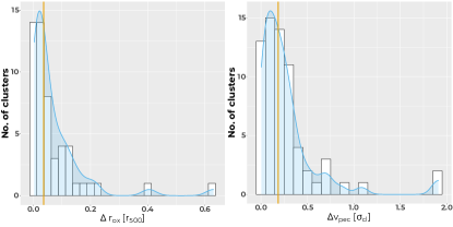
Figure 7: Left: Distribution of the relative projected positional offset of CDGs with respect to the X-ray peak ($\Delta r_{\mathrm{ox}}$). Right: distribution of the relative peculiar velocity of CDGs with respect to the cluster systemic velocity ($\Delta v_{\mathrm{pec}}$). The vertical yellow lines in the two panels are the thresholds separating relaxed form non-relaxed clusters.

In the right panel of Fig. 7, we trace the distribution for $\Delta v_{\mathrm{pec}}$. By definition of the CDG, in a dynamically relaxed system one would expect $\Delta v_{\mathrm{pec}}$ to tend to zero. However, assuming a typical upper threshold $\Delta v_{\mathrm{pec}}=$ 0.21, the percentage of clusters that have higher values is as high as 46% (31 out of 67). With a median $\Delta v_{\mathrm{pec}}=$ 0.185 $\sigma_{\mathrm{cl}}$, corresponding to a median $v_{\mathrm{pec}}$ of $\pm$ 147 km s^-1, once again it is clear that a high number of clusters cannot be assumed to have relaxed CDGs.

Codes for X-ray (inner region) and Offsets (core) are: [✓] Relaxed; [$\ast$] Disturbed; [$-$] No Data. References for ICM dynamical states are: Schuecker et al. (2001); Rines et al. (2001); Parekh et al. (2015); Vikhlinin et al. (2009); Ichinohe et al. (2019); Laganá et al. (2019); Tiwari & Singh (2021).

Codes for diffuse radio emission are: mini Radio-Halo [mH], Radio-Halo [H], Radio-Relic (shock) [R] and both halo and relic [HR].

Codes for cooling status of the core are: Strong cool-core [S], Weak-cool-core [W], Non-cool-core [N]; [s] indicates cold gas sloshing (cold gas front) is detected. References for core cooling status are: White (2001); Finoguenov et al. (2001); Chen et al. (2007); Sato et al. (2010); Lakhchaura & Singh (2014); Lovisari et al. (2015); Käfer et al. (2019).

Codes are: [u] unique CDG (choice of CDG is obvious, $\Delta m_{12}>0.5$); [b] binary central dominant BCGs (CDG is the most central or brightest), may also be a “Coma-like” system (BCG is brighter than CDG); [db] CDG is dumbell type; [far] binary dominant BCGs, but 2^nd-rank is far out of core radius; [m] multiple central dominant BCGs (3 or more BCGs inside 0.5 magnitud range); [n] weakly dominant CDG (giant elliptical); [fos] fossil group candidate BCG; [BSp] there is a bright spiral among the BCGs.

Table 5: Assembly state of the clusters.

IDcl	Innera	Radiob	CCc	$\Delta r_{\mathrm{ox}}$	$\Delta v_{\mathrm{pec}}$	Offsetsa	$\Delta m_{12}$	$\Delta r_{12}$	$\Delta m_{23}$	$\Delta r_{13}$	Commentsd
(1)	(2)	(3)	(4)	(5)	(6)	(7)	(8)	(9)	(10)	(11)	(12)
					U
A0122	$-$	$-$	$-$	0.062	0.342	$\ast$	0.000	0.01	1.618	0.41	b(db)
A0399	$\ast$	R	N	0.099	0.331	$\ast$	0.916	0.37	0.433	0.65	u
A0401	$\ast$	R	N	0.015	0.214	$\ast$	1.056	1.08	0.133	0.74	u
A1650	✓	$-$	W	0.025	0.100	✓	0.512	1.06	0.082	1.07	u
A1795	✓	mH?	S	0.011	0.095	✓	0.636	0.91	0.015	0.96	u
A2029	✓/$\ast$	mH	S,s	0.100	0.301	$\ast$	1.954	0.22	0.161	0.93	u
A2065	$\ast$	H?	W	0.045	0.044	$\ast$	0.000	0.02	0.054	0.09	m(db),For
A2244	$\ast$/✓	H	W	0.013	0.184	✓	1.025	1.11	0.186	0.92	u
A2670	$-$	$-$	W	0.035	0.342	$\ast$	1.131	0.71	0.183	0.93	u
A2798B	$-$	R	$-$	0.129	0.244	$\ast$	0.000	0.34	0.172	0.35	m(db)
A2801	$-$	$-$	N		0.025	$\ast$	1.125	0.39	0.080	0.60	u
A3094A	$-$	$-$	$-$	0.215	0.019	$\ast$	0.855	0.23	0.546	0.88	u
A3391	$\ast$	$-$	N	0.027	0.481	$\ast$	0.000	0.02	1.502	0.87	b(db)
A3562	$\ast$	H	W,s	0.046	0.211	$\ast$	0.330	1.07	0.795	0.45	u
					P
A0426A	$\ast$	mH	S,s	0.003	0.029	✓	0.436	0.11	0.407	0.07	b
A1060	$-$	$-$	W/S	0.007	0.166	✓	0.230	0.03	0.005	0.46	b,BSp
A1644	$\ast$	$-$	S,s	0.040	0.123	$\ast$	1.186	0.67	0.295	0.67	u
A1651	$\ast$	$-$	W	0.023	0.177	✓	1.128	0.58	0.097	0.35	u
A2063A	$\ast$/✓	R	W	0.018	0.040	✓	0.870	1.03	0.014	1.44	u
A2142	$\ast$	mH	W,s	0.030	0.241	$\ast$	0.295	0.17	-0.075	0.61	b
A2199	$\ast$	$-$	S,s	0.006	0.256	$\ast$	1.271	1.14	0.179	0.55	u
A3526A	$-$	$-$	S,s	0.005	0.078	✓	1.223	0.74	0.015	0.82	u
A3558	$\ast$	H	W,s	0.023	0.402	$\ast$	0.801	0.49	0.273	0.15	u
					L
A0634	$-$	$-$	$-$		0.019	✓	0.332	0.29	0.214	0.75	n
A3095	$-$	$-$	$-$		0.697	$\ast$	0.405	0.39	0.428	0.37	n
A4012A	$-$	$-$	$-$		0.013	✓	1.947	0.93	0.018	0.27	u
S0334	$-$	$-$	$-$		0.066	✓	0.359	0.04	0.587	0.10	n,For,BSp
S0336	$-$	$-$	$-$		0.581	$\ast$	0.514	0.38	0.352	0.23	n,Sp
S0906	$-$	$-$	$-$		1.082	$\ast$	0.732	0.20	0.367	0.47	u,BSp
					S
A0085A	$\ast$	R	S	0.007	0.031	✓	1.532	0.54	0.059	0.49	u
A0118	$-$	$-$	$-$		0.313	$\ast$	-0.228	0.12	0.467	0.49	b,For
A0119	$\ast$	$-$	N	0.133	0.024	$\ast$	0.532	0.13	0.194	0.75	u
A0133A	✓	R	S,s	0.036	0.255	$\ast$	1.506	0.17	0.036	1.23	u,For
A0400	$\ast$	$-$	N	0.061	0.450	$\ast$	0.000	0.01	1.175	0.10	b(db)
A0496	$\ast$	$-$	S,s	0.009	0.114	✓	1.126	0.85	0.087	0.90	u
A0539	$-$	$-$	N	0.008	0.520	$\ast$	0.000	0.01	0.404	0.28	m(db)
A0576	$\ast$	$-$	W	0.102	0.094	$\ast$	0.000	0.02	1.088	0.14	b(db)
A1656	✓	HR	N	0.051	0.157	$\ast$	-0.534	0.20	1.117	0.70	b,BSp
A1736A	$-$	$-$	$-$		0.017	✓	0.142	0.73	0.798	1.16	b(far)
A1736B	$\ast$	$-$	N	0.630	0.117	$\ast$	0.916	0.98	0.369	0.48	u
A2040B	$-$	$-$	$-$		0.283	$\ast$	0.727	0.51	0.080	0.40	u,For
A2052	$\ast$/✓	$-$	S,s	0.010	0.125	✓	0.928	0.92	0.072	0.22	u
A2204A	✓	mH	S,s	0.037	0.024	$\ast$	0.000	0.57	0.646	0.37	m(db)
A2255	$\ast$	HR	N	0.172	1.904	$\ast$	0.122	0.08	0.006	0.60	m
A2256	$\ast$	HR	N	0.115	0.163	$\ast$	0.107	0.18	0.000	0.07	m(db)
A2634	✓	$-$	W	0.069	0.204	$\ast$	0.102	0.79	0.914	0.55	u
A2811B	$-$	H	N	0.005	0.130	✓	0.828	1.00	0.049	1.09	u
A2877-70	$-$	$-$	W	0.044	0.100	✓	1.231	0.59	0.125	0.37	u
A3027A	$-$	$-$	$-$	0.158	0.061	$\ast$	-0.146	0.57	0.977	0.70	b(far),For
A3104	$-$	$-$	$-$	0.040	0.195	$\ast$	0.927	0.48	0.049	0.28	u
A3112B	✓	$-$	S	0.012	0.125	✓	1.070	0.91	0.646	0.74	u
A3158	$\ast$	$-$	N	0.018	0.361	$\ast$	0.268	0.08	0.755	0.18	b
A3526B	$-$	$-$	$-$		0.133	✓	0.450	0.73	1.099	0.74	u
A3530	$-$	$-$	N	0.083	0.185	$\ast$	1.002	0.06	0.798	0.89	b
A3532	✓	$-$	N	0.096	0.867	$\ast$	0.000	0.07	0.952	0.49	b(db)
A4038A-49	$\ast$	R	W	0.016	0.259	$\ast$	0.141	0.14	0.443	0.13	b,For
S0373	$-$	$-$	S,s	0.004	0.022	✓	0.159	0.43	0.306	0.06	u,For,BSp
					M
A0754	$\ast$	HR	N	0.209	0.223	$\ast$	0.933	0.42	0.139	0.41	u
A1367	$\ast$	R	N	0.405	0.301	$\ast$	0.511	0.66	0.030	0.86	b(far)
A2147	$\ast$	$-$	N	0.128	0.303	$\ast$	0.416	0.18	0.238	0.55	b,fos
A2151	$\ast$	$-$	$-$	0.005	1.910	$\ast$	-0.252	0.07	0.121	0.37	m,For
A2152A	$-$	$-$	$-$	0.073	0.004	$\ast$	0.408	0.76	0.541	0.80	n
A2197	$\ast$	$-$	W	0.033	0.672	$\ast$	0.823	1.07	0.409	0.95	u,For
A2804	$\ast$	$-$	N		0.214	$\ast$	0.051	0.50	0.165	0.65	b(far)
A3395	$\ast$	R	N	0.012	0.391	$\ast$	0.228	0.59	0.151	0.51	b(far)
A3556	$\ast$	$-$	$-$		0.054	$\ast$	0.339	0.75	0.315	0.23	b(far)
A3716	$\ast$	$-$	$-$		0.738	$\ast$	0.088	0.30	0.019	0.64	m

Note that, compared with the literature (e.g., Coziol et al., 2009; Lauer et al., 2014; Lopes et al., 2018), our median value for $\Delta v_{\mathrm{pec}}$ is relatively low. This is not due to a difference in sample but rather to a difference in the identification of the CDG. For example, in the cluster A2197, Lauer et al. (2014) assumed NGC 6173 is the BCG, instead of NGC 6160, which we identified as the real CDG. Since NGC 6173 turned out to be the SDG of a substructure of A2197 (A2197me in Appendix 0.7), its $v_{\mathrm{pec}}$ is naturally estimated to be higher than for NGC 6160. This emphasizes that a thorough analysis of the substructures in clusters is necessary to better determine the assembly state of the clusters. However, despite our careful analysis, the upgraded cluster peculiar velocities and velocity dispersion, we must still conclude that a significantly high number of nearby clusters do not have a relaxed core.

In fact, considering the clusters individually or in any of the assembly state class, we found no correlation between $\Delta r_{\mathrm{ox}}$ and $\Delta v_{\mathrm{pec}}$, as can be seen in Fig. 8 (compare, also, col. 21 with col. 22 of Table 3), a fact already noted in the literature (e.g., Lauer et al., 2014; De Propris et al., 2021). This advocates against the use of only one of these parameters as the proxy for the shift from the bottom of the cluster potential well, as proposed by, e.g., Lopes et al. (2018). In the present work we consider both together as indicators of the displacement of the CDG with respect to the bottom of the cluster potential well. Thus, we find that 70% of the clusters in our sample present significant disturbance in their mere core. The parameters $\Delta r_{\mathrm{ox}}$ and $\Delta v_{\mathrm{pec}}$ are reported respectively in cols. 5 and 6 of Table LABEL:T_Assembl. In col. 7, both offsets are used to classify the state of the CDG, adopting the same code as for col. 2, that is, the mark $\ast$ is assigned when any of them indicates dynamical disturbance.

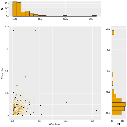
Figure 8: Distribution of offsets, parameterized.

To obtain a more comprehensive view of the impact of substructures, we show in Fig. 9 violin plots for $\Delta r_{\mathrm{ox}}$ and $\Delta v_{\mathrm{pec}}$, for each class of assembly state. In the upper left panel ($\Delta r_{\mathrm{ox}}$), the only trend visible is for the CDGs in the P class to lie below the threshold. This is confirmed for the pairs (U,P) and (P,S), a difference in the distribution being found using a Mann-Withney test at 95% CL, with $P=0.008$ and $P=0.025$, respectively. However, a Kruskal-Wallis test performed comparing the whole classes (with Dunn’s post-tests) found no statictically significant differences. Similarly, a Kruskal-Wallis test for $\Delta v_{\mathrm{pec}}$, in the upper right panel, is also negative, with $P=0.512$. Thus, we see no evidence for $\Delta r_{\mathrm{ox}}$ and $\Delta v_{\mathrm{pec}}$ to be related to the classes of assembly state.

Figure 9: Distributions of CDG parameters in different assembly classes (upper panel) and different core cooling status (lower panel): Left panels, $\Delta r_{ox}$, right panels, $\Delta v_{pec}$. In each graphic, the threshold for relaxation associated to the parameter is shown as a horizontal line.

In the lower panels of Fig. 9, we compare the distribution of $\Delta r_{\mathrm{ox}}$ (left) and $\Delta v_{\mathrm{pec}}$ (right) separating the clusters based on the core cooling status. Performing a Kruskal-Wallis test for $\Delta r_{\mathrm{ox}}$, we find a statistically significant difference between the NCC and SCC (with $P=0.011$) but not between NCC and WCC or WCC and SCC. However, for $\Delta v_{\mathrm{pec}}$ the difference is much more significant ($P\ll 0.0001$) between both NCC and SCC and NCC and SCC (but no difference between NCC and WCC as before). We find a 60% probability for WCC and NCC clusters to be associated with clusters that have both high $\Delta r_{\mathrm{ox}}$ and $\Delta v_{\mathrm{pec}}$, the trends being more obvious in S and M clusters than in U and P clusters. Considering that the latter two classes represent more massive clusters than the two former ones (cf. Table 4), the U and P clusters, consequently, are possibly slightly more relaxed than the S and M clusters. This is consistent with the complex assembly history of the clusters suggested by the assembly state classes. This correlation has already been pointed out in the literature: Zhang et al. (2011), for instance, found that the CDG–X-ray offset is related to the central cooling time of the clusters, for the HIFLUGCS X-ray flux limited galaxy cluster sample, suggesting that the system must be close to relaxed to have its cooling flow enhanced or a CC formed.

In general, the fact that the probability of association between the parameters related to the galaxies and gas in the core are not higher than 60% suggests that these two components most probably follow different paths towards equilibrium, the virialization time-scale, most specifically, being much smaller for the gas than for galaxies.

0.4.5 Results on the co-evolution of CDGs and clusters

The remaining columns in Table LABEL:T_Assembl are dedicated to report the evolutionary parameters for the CDGs: the magnitude gaps $\Delta m_{12}$ (col. 8) and $\Delta m_{23}$ (col. 10); the projected separation (clustercentric distance) of the 2^nd-rank, $\Delta r_{12}$, and 3^rd-rank, $\Delta r_{13}$ (cols. 9 and 11, respectively); and additional comments in column 12.

Using M_Ks as a proxy for the stellar mass of the CDG (e.g., Schneider, Gunn & Hoessel, 1983), we traced in the left panel of Fig. 10 its distribution for all the CDGs in our sample. A relatively good Gaussian fit suggests some level of similarity in the evolution of these CDGs. However, the distribution of the magnitude gaps, $\Delta m_{12}$, in the right panel of Fig. 10, is clearly bimodal, indicating different assembly histories for the CDGs themselves.

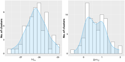
Figure 10: Distributions of CDGs properties: Left panel, CDG M_Ks, right panel, $\Delta m_{12}$.

This can also be appreciated in Fig. 11, which shows the distribution of absolute magnitudes for the CDGs and their respective second-rank galaxies as a function of the magnitude gaps $\Delta m_{12}$. As the gap increases, the luminosity of the CDG (its mass) grows almost linearly, while the luminosity of the second-rank galaxy slowly declines. Note that, due to our thorough analysis of substructures and definition of CDGs, it is not surprising that the change in mass we find is much faster than what was seen before (e.g., Smith et al., 2010). Although systems showing large magnitude gaps are consistent with a model where the CDG co-evolve with its cluster, the bimodality clearly suggests more complex assembly histories for the CDGs.

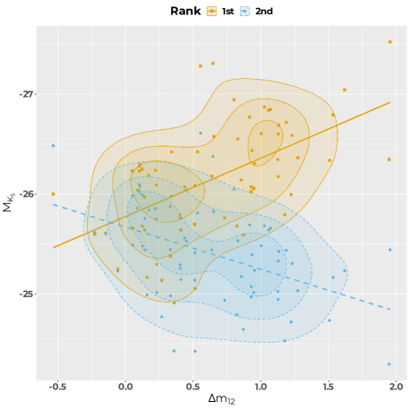
Figure 11: Distributions of absolute magnitudes for CDGs and 2^nd-rank galaxies as function of the magnitude gap.

To shed more light on the co-evolution of the CDGs and their clusters, we compare how the two magnitude gaps, $\Delta m_{12}$ and $\Delta m_{23}$, vary in the different assembly classes. This is done in the upper panels of Fig. 12. Although there is an apparent trend for U and P cluster to have higher magnitude gaps between the CDG and second-rank galaxy than for the S and M clusters, a Kruskal-Wallis test found no statistically significant difference ($P=0.190$). Similarly, a Kruskal-Wallis test found no statistically significant difference ($P=0.125$) for $\Delta m_{23}$.

Figure 12: Comparison of magnitude gaps in different assembly classes (upper panels and cooling states (lower panels).

In the lower panels of Fig. 12 we compare the two magnitude gaps for the different core cooling states. This time the Kruskal-Wallis test clearly identified a statistically significant difference for $\Delta m_{12}$, with $P=0.002$, between the pairs (NCC, SCC) and (WCC, SCC), but not for $\Delta m_{23}$. This is consistent with what we found before for $\Delta r_{\mathrm{ox}}$ and $\Delta v_{\mathrm{pec}}$. Consequenlty, despite the clear evidence of co-evolution of the clusters and their CDGs, especially in the core, the fact that the assembly state classes contain a mixture of core cooling states seems to confirm the complex assembly history of clusters in general.

0.5 Summary and conclusions

In this study we traced the assembly histories for a sample of 67 relatively rich (median $N_{c}=150$ spectroscopic members) and nearby ($z<0.15$) galaxy clusters, by classifying their level of substructuring in their outer regions (mostly beyond $r_{500}$) and estimating the dynamical impact of such subclumps on the host clusters. We also identified and characterized the dynamical properties of the CDGs of the clusters and compared them to the ICM equilibrium state, from X-ray literature data, mapped in the inner part and innermost core regions.

On the accompanying webpage, we offer the complete set of figures describing all clusters presented in this article: distribution of galaxies in each complex, system and significant substructure, projected number densities (like in Fig. 2), X-ray contour images (like in Fig. 3), CDG optical images, together with further information completing the data presented in the various tables included in the present article.

The following is a brief summary of our findings and conclusions:

• In 19% of the cluster in our sample, the classical BCG (directly identified from photometry) is not the CDG (gravitationally dominant galaxy). Among the discrepant cases we distinguish most specifically three different groups: binary central dominant galaxies with the second brightest as the CDG (Coma-like clusters), a BCG that is the SDG of a substructure (Fornax-like clusters), and clusters with a peripheric fossil candidate, where the BCG appears relatively isolated in the outskirt of the cluster.

• Using robust methods to determine cluster membership allowed us to more thoroughly determine the global dynamical parameters of the clusters: radial velocity of the system, velocity dispersion of galaxy members, virial mass and radius.

• Using different algorithms to detect substructures and estimate their gravitational impact on their host clusters, our analysis allowed us to determine that, although as many as 70% of nearby clusters show evidence of substructures, those dynamically significant only appear in 57% of the clusters.

• Based on the significance level of the impact of the substructure, we defined five classes of assembly states: high-mass, Unimodal (U); Low-mass unimodal (L); Multi-modal (M); Primary (P), with low-mass substructures attached to a main structure; and, finally, Substructured (S), formed by a main structure and high-mass substructures. We count 21% U, 13% P, 42% S, 15% M and 9% L clusters. In terms of masses, U and P clusters are more massive than S and M clusters, while L clusters are less massive, explaining why they are not detected in X-ray.

Our classification of clusters in terms of substructures seems consistent with a hierarchical model of formation, where clusters form by the mergers of groups of galaxies:

• U clusters are examples of massive systems that merged in the distant past and, consequently, their virialization process is well advanced.

• P clusters also formed in the past, and, because they are massive, they still accrete small groups from their environment.

• M and S clusters, which have significant substructures, are examples of relatively more recent mergers: in S clusters massive clumps are accreting smaller mass groups (minor mergers), while in M clusters the masses of the merging entities are comparable (major mergers).

• L clusters are the best examples of poor clusters in our sample: their masses and richness are comparable to those of massive groups, and, like the latter, are usually poor in gas. Their environment suggests some of them are either infalling or satellites of more massive clusters.

The classes can be interpreted as a “sequence” of different global assembly states possible for the clusters: they begin as a poor cluster (L) or a pile-up of small systems (M), then grow and pass to a state where a main structure starts to dominate (S), then become massive, although still accreting small groups (P), and finally become massive and regular/relaxed (U). Note that this is a snapshot of the assembly state, which can evolve in time: a U cluster can still accrete (becoming a P or S) or merge (becoming a M), for example. However, although there is a dispersion in masses, this dispersion is not that high. This is because the era of cluster evolution is relatively recent, and they did not have time to pass the process of a major merger much more than once or twice. Capturing smaller clumps (minor mergers), on the other hand, may have been frequent, but with smaller impact in their global masses. Also, the availability of new systems to be captured is decreasing with time because of the accelerated expansion of the Universe.

Our comparison of the properties of CDGs ($\Delta r_{\mathrm{ox}}$, $\Delta v_{\mathrm{pec}}$, $\Delta m_{12}$ and $\Delta m_{23}$) in the clusters with different assembly state classes and with the characteristics of the ICM in the inner region (different core cooling status) allows us to obtain a more precise view about the assembly process of the clusters.

• Considering the clusters individually or in any of the assembly states, we found no correlation between $\Delta r_{\mathrm{ox}}$ (CDG–X-ray offset) and $\Delta v_{\mathrm{pec}}$ (CDG peculiar velocity). We suggest the use of both together to characterize the dynamical state of the CDGs.

• We found a 60% probability for WCC and NCC clusters to be associated with clusters that have both high $\Delta r_{\mathrm{ox}}$ and $\Delta v_{\mathrm{pec}}$, the trends being more obvious in more massive clusters. Considering the difference in masses, this suggests U and P clusters are more relaxed than S and M clusters.

• Comparing how the two magnitude gaps, $\Delta m_{12}$ and $\Delta m_{23}$, vary in the different assembly states, we found only an apparent trend for U and P cluster to have higher magnitude gaps between the CDG and second-rank galaxy than the S and M clusters, while no trend is visible for $\Delta m_{23}$.

• However, we also found a significant difference for $\Delta m_{12}$, the gap being smaller in NCC and WCC than in SCC, while no difference is detected for $\Delta m_{23}$.

We conclude that, despite of clear evidence of co-evolution of the clusters and their CDGs, especially considering the gas in the core, the fact that the assembly state classes contain a mixture of core cooling states seems to confirm a complex assembly history of clusters. In general, the two baryonic components of clusters, galaxies and gas, probably follow different paths towards equilibrium, the relaxation time-scale, most specifically, being much smaller for the gas than for the galaxies. This difference implies that, even in the most evolved systems, the virialization and evolution of the CDG are complex processes that do not depend solely on time but also on the frequency and impact of mergers, cooling and heating of the ICM by shocks and feedback, cannibalism, pre-processing, among others. How much of this evolution is due to pre-processing in the initial groups, however, is still an open question.

0.6 New temperature measurements

We estimated the temperature for seven galaxy clusters of our sample using data from both XMM-Newton and Chandra (Table 6), four of which are previously unreported in the literature. This section briefly discusses the procedure for spectral fitting and computing temperatures.

7

Table 6: X-ray data for the targeted galaxy clusters.

Cluster	$z_{spec}$	X-ray peak	Telescope	Observation	Date of Observation	Exposure time
ID		$\alpha_{J2000},\delta_{J2000}$		ID		(ks)
(1)	(2)	(3)	(4)	(5)	(6)	(7)
A0122	0.113	00 57 24.7, -26 16 50	XMM	0504160101	2007 Dec 3	56.92
A2811	0.108	00 42 08.7, -28 32 09	XMM	0404520101	2006 Nov 28	25.91
A2870	0.024	01 07 43.2, -46 54 59	XMM	0205470301	2004 May 15	11.91
A0399	0.072	02 57 56.4, 13 00 59	Chandra	3230	2002 Nov 18	49.28
A3094	0.068	03 11 25.0, -26 53 59	Chandra	5799	2005 Nov 28	40.15
A3716	0.046	20 51 16.7, -52 41 43	Chandra	15133, 15583	2012 Dec 24/20	14.77, 16.08
A4038	0.028	23 47 43.2, -28 08 29	Chandra	4992	2004 Jun 28	33.97
1X-ray data obtained from XMM-Newton (http://nxsa.esac.esa.int/nxsa-web/) and Chandra (https://chandra.harvard.edu/). Columns: (1) Cluster ID; (2) spectroscopic redshift coming from NED (http://ned.ipac.caltech.edu); (3) Optical RA, Dec (J2000.0); (4) Telescope; (5) Observation ID; (6) Date of Observation; and (7) Exposure Time.

The data from XMM-Newton were reduced using the XMM-Newton Science Analysis Software (SAS), version 14.0.0. The raw data, downloaded in the form of observation data files (ODF), were processed in the following steps: i) Generation of calibrated event lists for the EPIC (MOS1, MOS2, and PN) cameras using the latest calibration data; this step was done using the SAS packages cifbuild, odfingest, epchain, and emchain. ii) Creation of the background light curves to identify time intervals with poor quality data, and filtering of the EPIC event lists to exclude periods of high background flaring and bad events. iii) Creation of a sky image of the filtered data set; these steps were performed using SAS packages evselect, tabgtigen, and xmm_select.

Finally, we extracted the spectra from the source and background using the task especget from SAS. This task produced two sets of files called the response matrix files (redistribution matrix file, RMF, and ancillary response file, ARF). Similarly, the Chandra data were obtained from the Chandra Data Archive (CDA) and operated by the Chandra Interactive Analysis of Observations CIAO, version 4.6.1, with calibration database version 4.6.1. In addition, the CIAO tool chandra_repro was applied to perform initial processing and obtain a new event file. These files are used for spectral fittings.

0.6.1 Spectral model fitting:

We extracted the spectra within a fixed radius of 0.5 $h_{70}^{-1}$ Mpc and excluded the point sources from this region. In some cases, the object was not centered on the observed field, such that we had to reduce the size of the extraction circle (see Table 7). The spectra from both, XMM-Newton and Chandra, were fitted using XSPEC spectral fitting software, version 12.5.1 (Arnaud, 1996). The photon counts of each cluster spectrum were grouped into bins with at least one count per bin. The spectral model was fitted to the data using the Ftools task grppha. The Galactic HI column (nH) was derived from the HI map from the Leiden/Argentine/Bonn (LAB) survey (Kalberla et al., 2005). This parameter was fixed while fitting the X-ray spectrum. The redshift of the spectral model was fixed to the cluster spectroscopic redshift coming from the NED database. Finally, we employed a fitting model to multiply a TBABS absorption model (Wilms et al., 2000) and a single-temperature optically thin thermal plasma component (the MEKAL code in XSPEC terminology, Mewe et al., 1986) to model the X-ray emission from ICM plasma.

4 Cluster Projected radius Physical radius $k$T_X (armin) (Mpc) (keV) (1) (2) (3) (4) A0122 4.0 0.5 3.70 $\pm$ 0.07 A2811 4.2 0.5 5.04 $\pm$ 0.05 A2870 8.6 0.25 1.07 $\pm$ 0.07 A0399 6.0 0.5 6.49 $\pm$ 0.27 A3094 6.4 0.5 3.15 $\pm$ 0.48 A3716N 4.6 0.25 2.19 $\pm$ 0.26 A3716S 4.6 0.25 3.65 $\pm$ 0.27 A4038 7.4 0.25 3.15 $\pm$ 0.05 1Columns: (1) Cluster ID; (2) radius used to extract spectra, (3) relative physical radius covered in the plan of sky, (4) estimated temperature from Model TBabs*mekal.

Table 7: Estimated X-ray temperatures for the targeted galaxy clusters.

0.7 List of m and hs substructures for P, S and M clusters.

Table 8: Substructures detected in the clusters of our sample. SDG: Substructure Dominant Galaxy

IDsub	RASDG	DecSDG	SDG	$N_{s}$	$v_{s}$	$\sigma_{s}$	$r_{200}$	$N_{\mathrm{a}}$	$v_{\mathrm{sub}}$	$\sigma_{\mathrm{sub}}$	$R_{\mathrm{p}}$	$R_{\mathrm{vir}}$	$M_{\mathrm{vir}}$
(1)	(2)	(3)	(4)	(5)	(6)	(7)	(8)	(9)	(10)	(11)	(12)	(13)	(14)
A2804mw	9.907535	$-$28.906199	6dF J0039377-285422	48	33790	323	0.631	27	33836	404	0.842	1.036	1.256
A2804me	10.008486	$-$28.902040	GALEX J004002.00-285407.9	32	32688	380	0.743	6	32268	314	0.540	0.757	0.487
A085Acw	10.376354	$-$9.262768	KAZ 364	22	14352	473	0.954	20	14414	482	0.529	1.019	1.121
A085Am	10.460515	$-$9.303040	MCG -02-02-086	272	16745	799	1.603	218	16738	852	1.813	2.242	12.000
A085Ase	10.792272	$-$9.861486	GIN 011	25	15083	272	0.547	15	15132	271	0.515	0.687	0.345
A2811Bm	10.537175	$-$28.535772	2MASX J00420892-2832087	123	32345	891	1.745	107	32340	947	1.766	2.345	14.500
A0118m	13.743478	$-$26.375153	2MASX J00545843-2622305	51	34586	702	1.369	46	34470	728	1.666	1.925	8.056
A0118c	13.874743	$-$26.396147	SARS 013.26663-26.66683	14	33958	338	0.660	13	33996	368	0.329	0.712	0.407
A0118e	13.958530	$-$26.365671	SARS 013.35062-26.63606	15	34171	584	1.139	15	34171	584	0.381	1.017	1.189
A0119m	14.067088	$-$1.255492	UGC 00579	277	13276	876	1.768	266	13281	893	1.302	2.080	9.488
A0119n	14.258582	$-$0.875172	UGC 00588	25	13402	450	0.909	23	13417	456	0.626	1.040	1.187
A0119ne	14.365250	$-$0.471357	GIN 021	23	13197	422	0.852	17	13188	461	0.651	1.062	1.263
A0133Anw	15.008555	$-$21.488472	ESO 541-G007	13	16585	474	0.951	13	16585	474	1.113	1.289	2.283
A0133Am	15.674046	$-$21.882154	ESO 541-G013	109	16762	723	1.453	87	16833	774	1.340	1.901	7.333
A0133Ane	15.999613	$-$21.372469	ESO 541-G016	10	17550	154	0.308	2	17436	205	0.698	0.630	0.267
A2870w	16.226784	$-$46.999523	2MASX J01045442-4659582	27	6396	329	0.672	24	6418	336	0.787	0.923	0.812
A2870e	16.927452	$-$46.907574	IC 1625	23	6919	235	0.480	17	6964	239	0.455	0.611	0.237
A2877m	17.481663	$-$45.931217	IC 1633	124	7231	647	1.318	99	7169	676	0.856	1.511	3.574
A3027Acw	37.482681	$-$33.177345	GALEX J022955.81-331036.6	24	23769	406	0.806	21	23821	423	1.054	1.164	1.721
A3027Am	37.706005	$-$33.103752	2dFGRS S518Z162	73	23283	697	1.384	63	23318	731	1.363	1.828	6.653
A0400m	44.423164	6.026997	NGC 1128	51	7011	336	0.684	42	7027	347	0.561	0.841	0.616
A0400ne	44.587616	6.095203	CGCG 415-046	10	6769	73	0.149	3	6768	94	0.228	0.260	0.018
A3104m	48.590549	$-$45.420238	LCRS B031238.4-453620	38	21784	446	0.887	28	21736	511	0.785	1.201	1.874
A3104e	49.033882	$-$45.391937	2MFGC 02678	10	21609	271	0.541	9	21589	278	0.698	0.769	0.493
A3104se	49.237873	$-$45.540817	LCRS B031514.7-454323	5	22160	125	0.248	2	22128	53	0.152	0.152	0.004
A3112Bn	49.472656	$-$44.041534	2MASX J03175343-4402295	7	23838	303	0.601	7	23838	303	0.718	0.819	0.601
A3112Bm	49.490250	$-$44.238213	ESO 248-G006	90	22549	596	1.185	56	22526	595	1.637	1.695	5.283
A0426Am	49.950980	41.511680	NGC 1275	297	5289	1023	2.092	296	5295	1024	1.322	2.309	12.700
S0373sw	50.674120	$-$37.208200	NGC 1316	20	1705	200	0.410	16	1728	230	0.238	0.484	0.115
S0373n	52.081950	$-$31.068180	NGC 1340	23	1283	249	0.513	16	1248	229	0.624	0.664	0.298
S0373m	54.621180	$-$35.450740	NGC 1399	178	1454	343	0.705	98	1458	390	0.307	0.748	0.427
A3158nw	55.549149	$-$53.390938	2MASX J03421179-5323273	16	18631	207	0.414	6	18711	104	0.541	0.367	0.053
A3158m	55.720634	$-$53.631302	ESO 156-G008 NED01	190	17373	1077	2.161	190	17373	1077	1.193	2.279	12.600
A3158cs	55.873669	$-$53.692135	2MASX J03432968-5341316	20	18594	287	0.575	15	18603	334	0.616	0.836	0.628
A0496nw	67.818871	$-$12.455068	IC 0377	36	9376	452	0.917	33	9384	468	0.943	1.219	1.890
A0496m	68.407669	$-$13.261956	MCG -02-12-039	315	9957	682	1.383	272	9933	715	1.330	1.812	6.210
A0539m	79.155548	6.440917	UGC 03274 NED05	110	8649	637	1.295	100	8645	674	0.982	1.576	4.073
A0539se	79.819481	5.757124	2MASX J05191667+0545256	15	8735	200	0.407	9	8777	243	0.646	0.694	0.348
A0539e	80.000107	6.680067	CGCG 421-028	7	8902	118	0.240	2	8809	69	0.428	0.261	0.018
A3395nw	96.518044	$-$54.029495	LEDA 423636	35	14534	614	1.238	34	14514	613	0.670	1.295	2.299
A3395m	96.901047	$-$54.449364	ESO 161-G008	166	14980	740	1.491	161	14995	746	1.032	1.703	5.241
A3395se	97.606720	$-$54.762615	ESO 161-IG012 NED01	13	14587	398	0.801	13	14587	398	0.544	0.905	0.786
A0576sw	108.784760	55.419525	CGCG 261-039	16	11328	305	0.618	5	11213	108	1.023	0.471	0.110
A0576m	110.375999	55.761581	CGCG 261-056 NED02	191	11359	861	1.743	183	11351	878	1.563	2.189	11.000
A0576ne	110.941490	56.581875	2MFGC 05892	13	11483	421	0.851	9	11474	231	1.051	0.787	0.512
A0754nw	136.941254	$-$9.392439	2MASX J09074590-0923327	24	16494	303	0.609	15	16487	295	0.615	0.770	0.488
A0754s	137.009079	$-$9.993835	2MASX J09080217-0959378	30	15827	541	1.088	30	15827	541	0.595	1.144	1.592
A0754mw	137.134949	$-$9.629739	2MASX J09083238-0937470	193	16168	820	1.647	173	16182	880	0.981	1.867	6.931
A0754me	137.330139	$-$9.699759	2MASX J09091923-0941591	118	16438	776	1.559	116	16450	782	0.881	1.665	4.922
A1060m	159.177963	$-$27.528584	NGC 3311	343	3698	676	1.385	323	3701	694	0.884	1.560	3.886
A1367mnw	176.009048	19.949820	NGC 3842	152	6546	512	1.045	122	6532	556	0.818	1.308	2.313
A1367mse	176.270782	19.606382	NGC 3862	117	6330	599	1.222	109	6309	608	0.882	1.424	2.979
A3526Am	192.203918	$-$41.311665	NGC 4696	210	3061	510	1.045	124	2991	569	0.817	1.332	2.414
A3526Bm	192.516449	$-$41.382072	NGC 4709	90	4563	276	0.566	47	4634	317	0.501	0.764	0.459
A3530m	193.900009	$-$30.347490	ESO 443-G011	101	16087	611	1.227	88	16105	633	1.195	1.601	4.367
A3530s1	193.929596	$-$30.718328	2MASX J12554310-3043059	9	15480	246	0.495	7	15509	256	0.511	0.660	0.306
A3532s2	193.980011	$-$30.721376	2MASX J12555520-3043169	7	16945	198	0.398	5	16878	163	0.574	0.506	0.139
A3532n	194.253647	$-$29.951527	2MASX J12570087-2957054	16	17021	279	0.561	9	17062	342	0.717	0.894	0.765
A3532m	194.341339	$-$30.363482	PKS 1254-30	80	16671	427	0.857	57	16700	443	0.908	1.151	1.628
A1644m	194.298248	$-$17.409575	2MASX J12571157-1724344	288	14077	1011	2.039	283	14088	1018	1.473	2.363	13.900
A1651m	194.843826	$-$4.196117	2MASX J12592251-0411460	177	25463	862	1.707	160	25465	877	1.808	2.262	12.700
A1656sw	194.351242	27.497778	NGC 4839	54	7412	404	0.822	54	7412	404	0.540	0.918	0.803
A1656m	194.898788	27.959389	NGC 4874	828	6921	1046	2.132	813	6927	1039	1.611	2.487	15.900
A3526Be	196.608917	$-$40.414490	ESO 323-G077	5	4615	101	0.208	4	4656	113	0.255	0.308	0.030
A3556m	201.027893	$-$31.669956	ESO 444-G025	102	14424	504	1.016	90	14436	520	1.047	1.346	2.586
A1736Anw	201.544220	$-$26.826834	6dF J1326106-264937	14	9974	158	0.321	6	9976	148	0.208	0.342	0.042
A1736Am	201.683777	$-$27.439398	ESO 509-G008	43	10500	271	0.549	18	10481	311	0.517	0.759	0.457
A1736Acn	201.898788	$-$27.042744	ESO 509-G016	8	10977	168	0.340	7	11059	186	0.449	0.512	0.141
A1736Ase	202.062210	$-$27.976803	MCG -05-32-027	9	9862	140	0.283	2	9850	23	0.172	0.091	0.001
A1736Bcn	201.703033	$-$27.143835	ESO 509-G009	28	14064	568	1.145	28	14064	568	0.505	1.120	1.488
A1736Bm	201.866852	$-$27.324682	IC 4252	107	13600	866	1.748	97	13572	878	1.372	2.092	9.668
A3558m	201.987015	$-$31.495474	ESO 444-G046	525	14408	953	1.920	448	14419	961	1.850	2.452	15.600
A2040Bsw	227.880768	7.251906	CGCG 049-033	14	13399	164	0.331	8	13330	211	0.649	0.631	0.265
A2040Bm	228.197815	7.434258	UGC 09767	136	13491	600	1.210	97	13584	663	1.309	1.708	5.263
A2052nw	228.094116	7.727029	CGCG 049-041	18	9881	253	0.514	8	9934	309	1.054	0.958	0.918
A2052m	229.185364	7.021667	UGC 09799	158	10355	588	1.192	120	10416	648	1.115	1.599	4.276
A2063Am	230.772095	8.609181	CGCG 077-097	189	10312	672	1.364	145	10347	758	1.196	1.818	6.284
A2142m	239.583450	27.233349	2MASX J15582002+2714000	182	27031	827	1.634	155	27046	830	1.745	2.152	11.000
A2147ms	240.570862	15.974513	UGC 10143	185	10706	854	1.732	178	10706	867	1.181	1.979	8.111
A2147mn	240.582687	16.346182	UGC 10144	210	11039	950	1.925	200	11030	964	1.479	2.288	12.600
A2147s	240.981934	14.902552	IC 1168	27	10564	467	0.946	15	10686	557	0.651	1.208	1.846
A2147se	241.606033	15.685868	UGC 10201	31	11740	489	0.989	31	11740	489	0.755	1.162	1.648
A2151sw	240.883575	17.198523	NGC 6034	32	10351	438	0.889	30	10348	434	0.552	0.968	0.950
A2151mw	241.148987	17.721445	NGC 6041	63	11006	871	1.764	63	11006	871	1.083	1.927	7.498
A2151mc	241.287537	17.729971	NGC 6047	92	10436	652	1.323	89	10434	663	0.645	1.353	2.589
A2151mn	241.566620	18.249800	NGC 6061	77	11186	341	0.691	57	11229	359	0.801	0.965	0.942
A2151e	241.663986	17.761154	IC 1194	22	11632	452	0.915	22	11632	452	0.371	0.870	0.692
A2152mnw	241.360168	16.442734	2MASX J16052644+1626338	56	13504	478	0.964	39	13480	466	0.857	1.172	1.698
A2152mse	241.371750	16.435793	UGC 10187 NED2	60	13126	255	0.514	19	13203	296	0.586	0.763	0.469
A2197mw	246.293030	40.892746	NGC 6146	67	8900	343	0.697	47	8870	331	0.782	0.909	0.782
A2197mc	246.921143	40.926899	NGC 6160	111	9575	463	0.939	64	9574	541	0.958	1.348	2.558
A2197me	247.436890	40.811710	NGC 6173	92	8786	395	0.802	68	8774	380	0.709	0.965	0.934
A2199m	247.159485	39.551380	NGC 6166	461	9086	785	1.595	441	9083	795	1.244	1.903	7.175
A2204Aw	247.792801	5.530654	2MASX J16311027+0531503	7	45236	371	0.710	7	45236	371	0.571	0.849	0.718
A2204An	248.111099	5.839127	2MASX J16322666+0550208	8	44975	264	0.507	4	45025	237	0.120	0.375	0.062
A2204Am	248.195404	5.575833	VLSS J1632.7+0534	77	45378	856	1.639	42	45406	1062	1.985	2.595	20.500
A2256cf	255.294220	78.726463	2MASX J17011061+7843352	27	17181	719	1.444	27	17181	720	0.599	1.384	2.832
A2256cb	255.700409	78.740837	2MASX J17024809+7844270	16	19704	250	0.500	12	19718	209	0.453	0.552	0.182
A2256m	256.113525	78.640564	UGC 10726	231	17530	1168	2.341	231	17530	1167	1.427	2.552	17.800
A2255sw	257.713409	63.853771	2MASX J17105121+6351135	12	24487	383	0.760	9	24556	442	0.567	0.974	1.011
A2255m	258.119812	64.060699	ZwCl 1710.4+6401A	155	24063	1072	2.128	154	24050	1069	1.564	2.465	16.300
A2255e	258.788116	64.048248	2MASX J17150914+6402536	14	24244	287	0.569	6	24078	206	0.599	0.597	0.232
A3716m	312.987152	$-$52.629829	ESO 187-G026	140	13509	744	1.501	123	13508	783	1.246	1.877	6.986
A2634sw	354.218323	26.509964	UGC 12708	13	9490	272	0.552	11	9434	268	0.646	0.741	0.425
A2634m	354.622437	27.031303	NGC 7720	172	9243	716	1.454	160	9235	736	1.217	1.796	6.031
A4038Am	356.937683	$-$28.140705	IC 5358	196	8872	725	1.474	166	8910	773	1.056	1.769	5.765
A4049s	357.903015	$-$28.365068	IC 5362	23	8307	270	0.549	23	8307	270	0.639	0.742	0.424
A4049n	357.976715	$-$27.929789	MCG -05-56-025	18	8809	88	0.180	6	8837	67	0.159	0.184	0.007

References

- Abbott et al. (2021) Abbott, T. M. C.; Adamów, M.; Aguena, M.; Allam, S.; Amon, A.; Annis, J.; et al. 2021, ApJS, 255:20
- Abdullah et al. (2020) Abdullah, M. H.; Wilson, G.; Klypin, A.; Old, L.; Praton, E; & Ali, G. B. 2020, ApJS, 246:2
- Abell et al. (1989) Abell, G. O.; Corwin Jr., H. G.; & Olowin, R. P. 1989, ApJS, 70, 1
- Ahn et al. (2012) Ahn, C. P.; Alexandroff, R.; Allende-Prieto, C.; Anderson, S. F.; Anderton, T.; Andrews, B. H.; et al. 2012, ApJS, 203:21
- Aihara et al. (2011) Aihara, H.; Allende-Prieto, C.; An, D.; Anderson, S. F.; Aubourg, É.; Balbinot, E.; et al. 2011, ApJS, 193:29
- Albareti et al. (2017) Albareti, F. D.; Allende-Prieto, C.; Almeida, A.; Anders, F.; Anderson, S.; Andrews, B. H.; et al. 2017, ApJS, 233:25
- Andernach et al. (2005) Andernach, H.; Tago, E; Einasto, M.; Einasto, J.; & Jaaniste, J. 2005, ASPC, 329, 283, eds. A.P. Fairall, P. Woudt, San Francisco: Astronomical Society of the Pacific
- Andrade-Santos et al. (2012) Andrade-Santos, F.; Lima-Neto, G. B.; & Laganá, T. F. 2012, ApJ, 746:139
- Andrade-Santos et al. (2017) Andrade-Santos, F.; Jones, C.; Forman, W. R.; et al. 2017, ApJ, 843:76
- Arnaud (1996) Arnaud, K. A. 1996, in Astronomical Society of the Pacific Conference Series, vol. 101, Astronomical Data Analysis Software and Systems V, ed. G.H. Jacoby & J. Barnes, 17.
- Baldry et al. (2010) Baldry, I. K.; Robotham, A. S. G.; Hill, D. T.; Driver, S. P.; Liske, J.; Norberg, P.; et al. 2010, MNRAS, 404, 86
- Barnes et al. (2001) Barnes, D. G.; Staveley-Smith, L.; de Blok, W. J. G.; Oosterloo, T.; Stewart, I. M.; Wright, A. E.; et al. 2001, MNRAS, 322, 486
- Bautz & Morgan (1970) Bautz, L. P.; & Morgan, W. W. 1970, ApJ, 162, L149
- Becker et al. (1995) Becker, R. H.; White, R. L.; & Helfand, D. J. 1995, ApJ, 450, 559
- Beers et al. (1982) Beers, T. C.; Geller, M. J.; & Huchra, J. P. 1982, ApJ, 257, 23
- Beers et al. (1990) Beers, T. C.; Flynn, K.; & Gebhardt, K. 1990, AJ, 100, 32
- Beers et al. (1992) Beers, T. C.; Gebhardt, K.; Huchra, J. P.; Forman, W.; Jones, C.; & Bothun, G. D. 1992, ApJ, 400, 410
- Benavides et al. (2020) Benavides, J. A.; Sales, L. V.; & Abadi, M. G. 2020, MNRAS, 498, 3852
- Bird & Beers et al. (1993) Bird, C. M.; & Beers, T. C. 1993, AJ, 105(4), 1596
- Bonjean et al. (2018) Bonjean, V.; Aghanim, N.; Salomé, P.; Douspis, M.; & Beelen, A. 2018, A&A, 609, A49
- Bonnarel et al. (2000) Bonnarel, F.; Fernique, P.; Bienaymé, O.; Egret, D.; Genova, F.; Louys, M.; Ochsenbein, F.; Wenger, M.; & Bartlett, J. G. 2000, A&A, 143, 33
- Botteon et al. (2022) Botteon, A.; Shimwell, T. W.; Cassano, R.; Cuciti, V.; Zhang, X.; Bruno, L.; et al. 2022, A&A, 660, A78
- Bravo-Alfaro et al. (2009) Bravo-Alfaro, H.; Caretta, C. A.; Lobo, C.; Durret, F.; & Scott, T. 2009, A&A, 495, 379
- Bryan & Norman (1998) Bryan, G. L.; & Norman, M. L. 1998, ApJ, 495, 80
- Buote & Tsai (1995) Buote, D. A.; & Tsai, J. C. 1995, ApJ, 452, 522
- Burenin et al. (2007) Burenin, R.A.; Vikhlinin, A.; Hornstrup, A.; Ebeling, H.; Quintana, H.; & Mescheryakov, A 2007, ApJS, 172, 561
- Caldwell et al. (1993) Caldwell, N.; Rose, J. A.; Sharples, R. M.; Ellis, R. S.; & Bower, R. G. 1993, AJ, 106, 473
- Caretta et al. (2008) Caretta, C. A.; Islas-Islas, J. M.; Torres-Papaqui, J. P.; Coziol, R.; Bravo-Alfaro, H.; & Andernach, H. 2008, Mem.S.A.It. 79, 1201
- Carlberg et al. (1997) Carlberg, R. G.; Yee, H. K. C; & Ellingson, E. 1997, ApJ, 478, 462
- Chambers et al. (2019) Chambers, K. C.; Magnier, E. A.; Metcalfe, N.; Flewelling, H. A.; Huber, M. E.; Waters, C. Z.; et al. 2019, eprint arXiv:1612.05560
- Chen et al. (2007) Chen, Y.; Reiprich, T.H.; Böhringer, H.; Ikebe, Y.; & Zhang, Y.-Y. 2007, A&A, 466, 805
- Chilingarian et al. (2010) Chilingarian, I. V.; Melchior, A. -L.; & Zolotukhin, I. Y. 2010, MNRAS, 405, 1409
- Chow-Martínez et al. (2014) Chow-Martínez, M.; Andernach, H.; Caretta, C. A.; & Trejo-Alonso, J. J. 2014, MNRAS, 445, 4073
- Chow-Martínez (2019) Chow-Martínez, M. 2019, PhD Thesis, Univ. Guanajuato, Mexico
- Cole et al. (2005) Cole, S.; Percival, W. J.; Peacock, J. A.; Norberg, P.; Baugh, C. M.; Frenk, C. S.; et al. 2005, MNRAS, 362, 505
- Condon et al. (1998) Condon, J. J.; Cotton, W. D.; Greisen, E. W.; Yin, Q. F.; Perley, R. A.; Taylor, G. B.; & Broderick, J. J. 1998, AJ, 115, 1693
- Coziol et al. (2009) Coziol, R.; Andernach, H.; Caretta, C. A.; Alamo-Martínez, K. A.; & Tago, E. 2009, AJ, 137, 4795
- Cruddace et al. (2002) Cruddace, R.; Voges, W.; Böhringer, H.; Collins, C. A.; Romer, A. K.; MacGillivray, H.; Yentis, D.; Schuecker, P.; Ebeling, H.; & De Grandi, S. 2002, ApJS, 140, 239
- Da Costa et al. (1998) Da Costa, L. N.; Willmer, C. N. A.; Pellegrini, P. S.; Chaves, O. L.; Rité, C.; Maia, M. A. G.; Geller, M. J.; Latham, D. W.; Kurtz, M. J.; Huchra, J. P.; Ramella, M.; Fairall, A. P.; Smith, C.; & Lípari, S. 1998, AJ, 116, 1
- De Propris et al. (2021) De Propris, R.; West, M. J.; Andrade-Santos, F.; Ragone-Figueroa, C.; Rasia, E.; Forman, W.; Jones, C.; Kipper, R.; Borgani, S.; García-Lambas, D.; Romashkova, E. A.; & Patra, K. C. 2021, MNRAS, 500, 310
- Dey (2019) Dey, A.; Schlegel, D. J.; Lang, D.; Blum, R.; Burleigh, K.; Fan, X.; et al. 2019, AJ, 157, id.168
- Donnari et al. (2021) Donnari, M.; Pillepich, A.; Joshi, G. D.; Nelson, D.; Genel, S.; Marinacci, F.; Rodriguez-Gomez, V.; Pakmor, R.; Torrey, P.; Vogelsberger, M.; & Hernquist, L. 2021, MNRAS, 500, 4004
- Dressler (1980) Dressler,A. 1980, ApJ, 236, 351
- Dressler & Shectman (1988) Dressler, A.; & Shectman, S. A. 1988, AJ, 95, 985
- Dupuy et al. (2019) Dupuy, A.; Courtois, H. M.; Dupont, F.; Denis, F.; Graziani, R.; Copin, Y.; Pomarède, D.; Libeskind, N.; Carlesi, E.; Tully, B.; & Guinet, D. 2019, MNRAS, 489, L1
- Ebeling et al. (1996) Ebeling, H.; Voges, W.; Böhringer, H.; Edge, A. C.; Huchra, J. P.; & Briel, U. G. 1996, MNRAS, 281, 799
- Einasto et al. (2010) Einasto, M.; Tago, E.; Saar, E.; Nurmi, P.; Enkvist, I.; Einasto, P.; et al. 2010, A&A, 522, A92
- Einasto et al. (2012) Einasto, M.; Vennik, J.; Nurmi, P.; Tempel, E.; Ahvensalmi, A.; Tago, E.; Liivamägi, L. J.; Saar, E.; Heinämäki, P.; Einasto, J.; & Martínez, V. J. 2012, A&A, 540, A123
- Einasto et al. (2014) Einasto, M.; Lietzen, H.; Tempel, E.; Gramann, M.; Liivamägi, L. J.; & Einasto, J. 2014, A&A, 562, A87
- Falco et al. (1999) Falco, E. E.; Kurtz, M. J.; Geller, M. J.; Huchra, J. P.; Peters, J.; Berlind, P.; Mink, D. J.; Tokarz, S. P.; & Elwell, B. 1999, PASP, 111, 438
- Finoguenov et al. (2001) Finoguenov, A.; Arnaud, M.; & David, L. P. 2001, ApJ, 555, 191
- Fitchett & Webster (1987) Fitchett, M.; & Webster, R. 1987, ApJ, 317, 653
- Fitzpatrick (1999) Fitzpatrick, E. L. 1999, PASP, 111, 63
- Flin & Krywult (2006) Flin, P.; & Krywult, J. 2006, A&A, 450, 9
- Fraser-McKelvie et al. (2011) Fraser-McKelvie, A.; Pimbblet, K. A.; & Lazendic, J. S. 2011, MNRAS, 415, 1961
- Fukazawa et al. (2004) Fukazawa, Y.; Makishima, K.; & Ohashi, T. 2004, PASJ, 56, 965
- Fukugita et al. (1995) Fukugita, M.; Shimasaku, K.; & Ichikawa, T. 1995, PASP, 107, 945
- Geller & Beers (1982) Geller, M. J.; & Beers, T. C. 1982, PASP, 94, 421
- Gregory & Thompson (1984) Gregory, S. A.; & Thompson, L. A. 1984, ApJ, 286, 422
- Haggar et al. (2023) Haggar, R.; Kuchner, U.; Gray, M. E.; Pearce, F. R.; Knebe, A.; Yepes, G.; & Cui, W. 2023, MNRAS, 518, 1316
- Hambly et al. (2001a) Hambly, N. C.; MacGillivray, H. T.; Read, M. A.; Tritton, S. B.; Thomson, E. B.; Kelly, B. D.; Morgan, D. H.; Smith, R. E.; Driver, S. P.; Williamson, J.; Parker, Q. A.; Hawkins, M. R. S.; Williams, P. M.; & Lawrence, A. 2001a, MNRAS, 326, 1279
- Hambly et al. (2001b) Hambly, N. C.; Irwin, M. J.; & MacGillivray, H. T. 2001b, MNRAS, 326, 1295
- Hambly et al. (2001c) Hambly, N. C.; Davenhall, A. C.; Irwin, M. J.; & MacGillivray, H. T. 2001c, MNRAS, 326, 1315
- Harvey et al. (2017) Harvey, D.; Courbin, F.; Kneib, J. P.; & McCarthy, I. G. 2017, MNRAS, 472, 1972
- Hou et al. (2009) Hou, A.; Parker, L. C.; Harris, W. E.; & Willman, D. J. 2009, ApJ, 702, 1199
- Huchra et al. (2012) Huchra, J. P.; Macri, L. M.; Masters, K. L.; Jarrett, T. H.; Berlind, P.; Calkins, M.; et al. 2012, ApJS, 199:26
- Hudson et al. (2010) Hudson, D. S.; Mittal, R.; Reiprich, T.H.; Nulsen, J.; Andernach, H.; & Sarazin, C. L. 2010, A&A, 513, A37
- Ichinohe et al. (2019) Ichinohe, Y.; Simionescu, A.; Werner, N.; Fabian, A.C.; & Takahashi, T. 2019, MNRAS, 483, 1744
- Ikebe et al. (2002) Ikebe, Y.; Reiprich, T. H.; Böhringer, H.; Tanaka, Y.; & Kitayama, T. 2002, A&A, 383, 773
- Islas-Islas et al. (2015) Islas-Islas, J. M. 2015, PhD Thesis, Univ. Guanajuato, Mexico
- Jarrett et al. (2000) Jarrett, T. H.; Chester, T.; Cutri, R.; Schneider, S.; Skrutskie, M.; & Huchra, J. P. 2000, AJ, 119, 2498
- Jarrett et al. (2003) Jarrett, T. H.; Chester, T.; Cutri, R.; Schneider, S. E.; & Huchra, J. P. 2003, AJ, 125, 525.
- Jarrett (2004) Jarrett, T. H. 2004, PASA, 21, 396
- Jeltema et al. (2005) Jeltema, T. E.; Canizares, C. R.; Bautz, M. W.; & Buote, D. A. 2005, ApJ, 624, 606
- Jones & Forman (1999) Jones, C., & Forman, W. 1999, ApJ, 511, 65
- Jones et al. (2009) Jones, D. H.; Read, M. A.; Saunders, W.; Colless, M.; Jarrett, T.; Parker, Q. A.; et al. 2009, MNRAS, 399, 683
- Käfer et al. (2019) Käfer, F.; Finoguerov, A.; Eckert, D.; Sanders, J. S.; Reiprich, T. H.; & Nandra, K. 2019, A&A, 628, A43
- Kalberla et al. (2005) Kalberla, P. M. W.; Burton, W. B.; & Hartmann, D. 2005, A&A, 440, 775
- Knowles et al. (2022) Knowles, K.; Cotton, W. D.; Rudnick, L.; Camilo, F.; Goedhart, S.; Deane, R.; et al. 2022, A&A, 657, A56
- Kopylova & Kopylov (2018) Kopyova, F. G.; & Kopylov, A. I. 2018, Ap. Bull., 73(3), 267
- Kowalski et al. (1984) Kowalski, M. P.; Ulmer, M. P.; Cruddace, R. G.; & Wood, K. S. 1984, ApJS, 56, 403
- Krempéc-Krygier et al. (2002) Krempéc-Krygier, J.; Krygier, B.; & Krywult, J. 2002, Baltic Astr., 11, 269
- Kriessler & Beers (1997) Kriessler, J. R.; & Beers, T. C. 1997, AJ, 113, 80
- Lacy et al. (2020) Lacy, M.; Baum, S. A.; Chandler, C. J.; Chatterjee, S.; Clarke, T. E.; Deustua, S.; et al. 2020, PASP, 132, 5001
- Laganá et al. (2019) Laganá, T. F.; Durret, F.; & Lopes, P. A. A. 2019, MNRAS, 484, 2807
- Lakhchaura & Singh (2014) Lakhchaura K. & Singh K.P. 2014, AJ, 147:156
- Lauer et al. (2014) Lauer, T. R.; Postman, M.; Strauss, M. A.; Graves, G. J.; & Chisari, N. 2014, ApJ, 797:82
- Lavoie et al. (2016) Lavoie, S.; Willis, J. P.; Démoclès, J.; Eckert, D.; Gastaldello, F.; Smith, G. P.; et al. 2016, MNRAS, 462, 4141
- Ledlow et al. (2003) Ledlow, M. J.; Voges, W.; Owen, F. N.; & Burns, J. O. 2003, AJ, 126, 2740
- Li & Chen (2019) Li, Y.-T.,; & Chen, L.-W. 2019, MNRAS, 482, 4084
- Limber & Mathews (1960) Limber, D. N.; & Mathews, W. G. 1960, ApJ, 132, 286
- Lisker et al. (2018) Lisker, T.; Vijayaraghavan, R.; Janz, J.; Gallagher III, J. S.; Engler, C.; & Urich, L 2018, ApJ, 865:40
- Liu et al. (2018) Liu, A.; Yu, H.; Diaferio, A.; Tozzi, P.; Hwang, H. S.; & Umetsu K. 2018, ApJ, 863:102
- Lopes et al. (2006) Lopes, P. A. A.; De Carvalho, R. R.; Capelato, H. V.; Gal, R. R.; Djorgovski, S. G.; Brunner, R. J.; Odewahn, S. C.; & Mahabal A. A. 2006, ApJ, 648, 209
- Lopes et al. (2018) Lopes, P. A. A.; Trevisan, M.; Laganá, T. F.; Durret, F.; Ribeiro, A. L. B.; & Rembold, S. B. 2018, MNRAS, 478, 5473
- López-Gutiérrez et al. (2022) López-Gutiérrez, M. M.; Bravo-Alfaro, H.; van Gorkom, J. H.; Caretta, C. A.; Durret, F.; Núñez-Beltrán, L. M.; Jaffé, Y. L.; Hirschmann, M.; & Pérez-Millán, D. 2022, MNRAS, 517, 1218
- Lovisari et al. (2015) Lovisari, L.; Reiprich, T.H.; & Schellenberger, G. 2015, A&A, 573, A118
- Martel et al. (2014) Martel, H.; Robichaud, F.; & Barai, P. 2014, ApJ, 786:79
- McNamara et al. (1996) McNamara, B. R.; Wise, M.; Sarazin, C. L.; Jannuzi, B. T.; & Elston, R. 1996, ApJ, 466, L9
- Merritt (1985) Merritt, D. 1985, ApJ, 289, 18.
- Mewe et al. (1986) Mewe, R.; Lemen, J. R.; & Van den Oord, G. H. J. 1986, A&AS, 65, 511
- Migkas et al. (2020) Migkas, K.; Schellenberger, G.; Reiprich, T. H.; Pacaud, F.; Ramos-Ceja, M. E.; & Lovisari, L. 2020, A&A, 636, A15
- Mihos (2004) Mihos, J. C. 2004, in Clusters of Galaxies: Probes of Cosmological Structure and Galaxy Evolution, 277
- Mohr et al. (1993) Mohr, J. J.; Fabricant, D. G.; & Geller, M. J. 1993, ApJ, 413, 492
- Obayashi et al. (1998) Obayashi, H.; Makishima, K.; & Tamura, T. 1998, PASJ, 50, 537
- Oegerle & Hill (2001) Oegerle, W. R.; & Hill, J. M. 2001, AJ, 122, 2858
- Ota et al. (2006) Ota, N.; Kitayama, T.; Masai, K.; & Mitsuda, K. 2006, ApJ, 640, 673
- Parekh et al. (2015) Parekh, V.; van der Heyden, K.; Ferrari, C.; Angus, G.; & Holwerda, B. 2015, A&A, 575, A127
- Pearson & Batuski (2013) Pearson, D. W.; & Batuski, D. J. 2013, MNRAS, 436, 796
- Piffaretti & Valdarnini (2008) Piffaretti, R.; & Valdarnini, R. 2008, A&A, 491, 71
- Piffaretti et al. (2011) Piffaretti, R.; Arnaud, M.; Pratt, G. W.; Pointecouteau, E.; & Melin, J. -B. 2011, A&A, 534, A109
- Pinkney et al. (1996) Pinkney, J.; Roettiger, K.; Burns, J. O.; & Bird, C. M. 1996, ApJS, 104, 1
- Pisani (1996) Pisani, A. 1996, MNRAS, 278, 697
- Planck Collab. (2011) Planck Collaboration 2011, A&A, 536, A11
- Planck Collab. (2014) Planck Collaboration 2014, A&A, 571, A29
- Planck Collab. (2016) Planck Collaboration 2016, A&A, 594, A27
- Poggianti et al. (2006) Poggianti, B. M.; von der Linden, A.; De Lucia, G.; Desai, V.; Simard, L.; Halliday, C.; Aragón-Salamanca, A.; Bower, R.; Varela, J.; Best, P.; Clowe, D. I.; Dalcanton, J.; Jablonka, P.; Milvang-Jensen, B.; Pello, R.; Rudnick, G.; Saglia, R.; White, S. D. M.; & Zaritsky, D. 2006, ApJ, 642, 188
- Porter et al. (2008) Porter, S. C.; Raychaudhury, S.; Pimbblet, K. A.; & Drinkwater, M. J. 2008, MNRAS, 388, 1152
- Poudel et al. (2017) Poudel, A., Heinämäki, P.; Tempel, E.; Einasto, M.; Lietzen, H.; & Nurmi, P. 2017, A&A, 597, A86
- Predehl et al. (2021) Predehl, P.; Andritschke, R., Arefiev, V.; Babyshkin, V.; Batanov, O.; Becker, W.; et al. 2021, A&A, 647, A1
- Ramella et al. (2007) Ramella, M.; Biviano, A.; Pisani, A.; Varela, J.; Bettoni, D.; Couch, W. J.; D’Onofrio, M.; Dressler, A.; Fasano, G.; Kjørgaard, P.; Moles, M.; Pignatelli, E.; Poggianti, B. M. 2007, A&A, 470, 39
- Regös & Geller (1989) Regös, E.; & Geller, M. J. 1989, ApJ, 98, 755
- Reiprich et al. (2021) Reiprich, T. H.; Veronica, A.; Pacaud, F.; Ramos-Ceja, M. E.; Ota, N.; Sanders, J.; et al. 2021, A&A, 647, A2
- Rines et al. (2001) Rines, K.; Mahdavi, A.; Geller, M.J.; Diaferio, A.; Mohr, J.J.; & Wegner, G. 2001, ApJ, 555, 558
- Rood & Sastry (1971) Rood, H. J.; & Sastry, G. N. 1971, PASP, 83, 313
- Rumbaugh et al. (2018) Rumbaugh, N.; Lemaux, B. C.; Tomczak, A. R.; Shen, L.; Pelliccia, D.; Lubin, L. M.; Kocevski, D. D.; Wu, P. -F.; Gal, R. R.; Mei, S.; Fassnacht, C. D.; Squires, G. K. 2018, MNRAS, 478, 1403
- Santiago-Bautista et al. (2020) Santiago-Bautista, I.; Caretta, C. A.; Bravo-Alfaro, H.; Pointecouteau, E.; & Andernach, H. 2020, A&A, 637, A31
- Sargent & Turner (1977) Sargent, W. L. W.; & Turner, E. L. 1977, ApJ, 212, L3
- Sato et al. (2010) Sato, K.; Kelley, R. L.; Takei, Y.; Tamura, T.; Yamasaki, N. Y.; Ohashi, T.; Gupta, A.; & Galeazzi, M. 2010, PASJ, 62, 1423
- Schlafly & Finkbeiner (2011) Schlafly, E. F.; & Finkbeiner, D. P. 2011, ApJ, 737:103
- Schlegel et al. (1998) Schlegel, D. J.; Finkbeiner, D. P.; & Davis, M. 1998, ApJ, 500, 525
- Schneider, Gunn & Hoessel (1983) Schneider, D. P.; Gunn, J. E.; & Hoessel, J. G. 1983, ApJ, 264, 337
- Schuecker et al. (2001) Schuecker, P.; Böhringer, H.; Reiprich, T.H.; & Feretti, L. 2001, A&A, 378, 408
- Serna & Gerbal (1996) Serna, A.; & Gerbal, D. 1996, A&A, 309, 65
- Shanks et al. (2015) Shanks, T.; Metcalfe, N.; Chehade, B.; Findlay, J. R.; Irwin, M. J.; Gonzalez-Solares, E.; Lewis, J. R.; Kupcu-Yoldas, A.; Mann, R. G.; Read, M. A.; Sutorius, E. T. W.; & Voutsinas, S. 2015, MNRAS, 451, 4238
- Shectman et al. (1996) Shectman, S. A.; Landy, S. D.; Oemler, A.; Tucker, D. L.; Lin, H.; Kirshner, R. P.; & Schechter, P. L. 1996, ApJ, 470, 172
- Skrutskie et al. (2006) Skrutskie, M. F.; Cutri, R. M.; Stiening, R.; Weinberg, M. D.; Schneider, S.; Carpenter, J. M.; Beichman, C.; Capps, R.; Chester, T.; Elias, J.; Huchra, J.; Liebert, J.; Lonsdale, C.; Monet, D. G.; Price, S.; Seitzer, P.; Jarrett, T.; Kirkpatrick, J. D.; Gizis, J.; Howard, E.; Evans, T.; Fowler, J.; Fullmer, L.; Hurt, R.; Light, R.; Kopan, E. L.; Marsh, K. A.; McCallon, H. L.; Tam, R., Van Dyk, S.; & Wheelock, S. 2006, AJ, 131, 1163
- Smith et al. (2010) Smith, G. P.; Khosroshahi, H. G., Dariush, A.; Sanderson, A. J. R.; Ponman, T. J.; Stott, J. P.; Haines, C. P.; Egami, E.; & Stark, D. P. 2010, MNRAS, 409, 169
- Song et al. (2017) Song, H.; Hwang, H. S.; Park, C.; & Tamura, T. 2017, ApJ, 842:88
- Stewart et al. (1984) Stewart, G. C.; Fabian, A. C.; Jones, C.; & Forman, W. 1984, ApJ, 285, 1
- Stott et al. (2010) Stott, J. P.; Collins, C. A.; Sahlén, M.; Hilton, M.; Lloyd-Davies, E.; Capozzi, D.; et al. 2010, ApJ, 718, 23
- Struble & Rood (1982) Struble, M. F.; & Rood, H. J. 1982, AJ, 87, 7
- Tempel et al. (2009) Tempel, E.; Einasto, J.; Einasto, M.; Saar, E.; & Tago E. 2009, A&A, 495, 37
- Tiwari & Singh (2021) Tiwari, J.; & Singh, K. P. 2021, MNRAS, 500, 5524
- Tonry (1985) Tonry, J. L. 1985, AJ, 90, 2431
- Trejo-Alonso et al. (2014) Trejo-Alonso, J. J.; Caretta, C. A.; Laganá, T. F.; Sodré Jr., L.; Cypriano, E. S.; Lima Neto, G. B.; & Mendes de Oliveira, C. 2014, MNRAS, 441, 776
- Tyler et al. (2014) Tyler, K. D.; Bai, L.; & Rieke, G. H. 2014, ApJ, 794:31
- Van Weeren et al. (2019) Van Weeren, R. J.; de Gasperin, F.; Akamatsu, H.; Brüggen, M.; Feretti, L.; Kang, H.; Stroe, A.; & Zandanel, F. 2019, Space Sci. Rev. 2015:16
- Varela et al. (2012) Varela, J.; Betancort-Rijo, J.; Trujillo, I.; & Ricciardelli E. 2012, ApJ, 744:82
- Vikhlinin et al. (1998) Vikhlinin, A.; McNamara, B.R.; Forman, W.; Jones, C.; Quintana, H.; & Hornstrup, A. 1998, ApJ, 502, 558
- Vikhlinin et al. (2009) Vikhlinin, A.; Burenin, R. A.; Ebeling, H.; Forman, W. R.; Hornstrup, A.; Jones, C.; Kravtsov, A. V.; Murray, S. S.; Nagai, D.; Quintana, H.; & Voevodkin, A. 2009, ApJ, 692, 1033
- Wen & Han (2013) Wen, Z. L.; & Han, J. L. 2013, MNRAS, 436, 275
- Wen & Han (2015) Wen, Z. L.; & Han, J. L. 2015, ApJ, 807:178
- West et al. (1988) West, M. J.; Oemler-Jr., A.; & Dekel, A. 1988, ApJ, 327, 1
- White (2001) White, D.A. 2001, MNRAS, 312, 663
- Wilms et al. (2000) Wilms, J.; Allen, A.; & McCray, R. 2000, ApJ, 542, 914
- Yu et al. (2015) Yu, H.; Serra, A. L.; Diaferio, A.; & Baldi, M. 2015, ApJ, 810:37
- Yuan et al. (2005) Yuan, Q. -R.; Yan, P. -F.; Yang, Y. -B.; & Zhou, X. 2005, Chin. J. Astron. Astrophys. 5, 126
- Zhang et al. (2011) Zhang, Y. -Y.; Andernach, H.; Caretta, C. A.; Reiprich, T. H.; Böhringer, H.; Puchwein, E.; Sijacki, D.; & Girardi, M. 2011, A&A, 526, A105
- Zhao et al. (2015) Zhao, D.; Aragón-Salamanca, A.; & Conselice, C. J. 2015, MNRAS, 453, 4444