Testing gravity with gauge-invariant polarization states of gravitational waves

Abstract

The determination of the polarization modes of gravitational waves (GWs), and of their dispersion relations is decisive to scrutinize the viability of extended theories of gravity. A tool to investigate the polarization states of GWs is the Newman-Penrose (NP) formalism. However, if the speed of GWs is smaller than the speed of light, the number of NP variables is greater than the number of polarizations. To overpass this inconvenience we use the Bardeen formalism to describe the six possible polarization modes of GWs considering different general dispersion relations for the modes. The definition of a new gauge-invariant quantity enables an unambiguous description of the scalar longitudinal polarization mode. We apply the formalism to General Relativity, scalar-tensor theories, and $f(R)$-gravity. To obtain a bridge between theory and experiment, we derive an explicit relation between a physical observable (the derivative of the frequency shift of an electromagnetic signal) with the gauge-invariant variables. From this relation, we find an analytical formula for the Pulsar Timing rms response to each polarization mode. To estimate the sensitivity of a single Pulsar Timing we focus on the case of a dispersion relation of a massive particle. The sensitivity curves of the scalar longitudinal and vector polarization modes change significantly depending on the value of the effective mass. The detection (or absence of detection) of the polarization modes using the Pulsar Timing technique has decisive implications for alternative theories of gravity. Finally, the investigation of a cutoff frequency in the Pulsar Timing band can lead to a more stringent bound on the graviton mass than that presented by ground-based interferometers.

• August 2023

1 Introduction

The gravitational wave (GW) events detected so far by the Advanced LIGO and Advanced Virgo interferometers have shown their ability to impact our knowledge of physics and astrophysics. These observations offer a unique opportunity to test General Relativity (GR) in the dynamical regime.

All the extensions to Einstein’s theory predict modifications to the conventional GW signal due to one or more of three aspects, namely, changes in the waveform due to particularities in the generation mechanism, changes in the propagation due to new dispersion relations or differences in the interaction of the wave with the background geometry, and the number of independent polarization states of GWs.

Considering these effects, tests of gravity performed with the data of the three observing runs of Advanced LIGO and Advanced Virgo have shown that all the observed events are consistent with GR [1, 2, 3]. However, the planned increase in the sensitivity of the detectors, the new generations of interferometers, the pulsar timing technique and the future space-based GW detectors as LISA will be able to produce stringent tests to GR.

In the case of the polarization states of GWs, a detection indicating the presence of a polarization mode beyond the usual plus and cross polarizations would imply a violation of Einstein’s theory. In general, an alternative theory of gravity in four dimensions can predict up to six polarization modes of GWs, namely, two tensor, two vector, one scalar transversal, and one scalar longitudinal [4, 5].

To check the presence or absence of such modes in a specific theory it is appropriate to consider the evaluation of gauge invariant quantities to warrant that they are related to truly physical observables. The most common strategy is to use the Newman-Penrose (NP) formalism [4, 5]. Within the NP formalism, one can describe the irreducible parts of the Riemann tensor in the linearized regime. In such a framework, two real and two complex variables describe the polarization states of GWs in any four-dimensional metric theory of gravity. The NP formalism has been applied in the scope of several theories to reveal the polarization properties of GWs (see, e.g., [6, 7, 8, 9, 10, 11, 12, 13, 14, 15, 16, 17, 18, 19]).

In recent years, however, some criticisms have been raised in the literature regarding the use of the original NP formalism in theories that present one or more massive modes in the linearized regime [20, 21, 22, 23]. This is the case of a huge class of alternative theories, including the massive version of the Brans-Dicke theory [8], Horndeski theory [22] and $f(R)$-gravity [7, 12, 20]. The main criticism is related to the fact that if GWs travel at a speed different from the speed of light, then other NP quantities, beyond the original four, would be non-null. As a consequence, the original NP formalism would be incomplete and could result in misleading conclusions for some theories. Thus, to have a complete description of the polarizations one needs new NP variables in this case. In fact, to describe six polarizations there are not only four but nine variables representing fourteen components of the Riemann tensor [23]. Certainly, some variables could be more important than others depending on the dispersion relation and frequency.

However, there is a gauge-invariant alternate formalism to identify the polarization modes in a metric theory of gravity. It consists in decompose the metric into irreducible components according to their properties under spatial rotation [(3+1) decomposition] and then constructing gauge-invariant combinations of the metric perturbations. In the scope of cosmological perturbation theory such quantities are known as Bardeen variables [24, 25]. Recently, Wagle et al. [17] used these gauge-invariant variables to study the polarizations of GWs in the context of two theories, namely, the dynamical Chern-Simons gravity and the Einstein-dilaton-Gauss-Bonnet gravity. They have found that the NP formalism and the (3+1) decomposition lead to the same result in both cases. The formalism of Bardeen variables has the advantage that the same number of variables are applicable to describe the polarization modes of GWs to any frequency.

In the present work, we review the Bardeen formalism and show how it can be applied in the identification of the polarization modes of GWs for any metric theory of gravity. We show that different from the case of the NP quantities, we have six variables to describe six polarizations, i.e., the number of variables is not related to the dispersion relation of GWs. In order to describe the scalar longitudinal polarization mode we define a new gauge-invariant variable as a combination of the usual Bardeen scalar variables.

We also obtain the frequency shift of a light signal induced by GWs in terms of the Bardeen variables in such a way that the final result is valid for any dispersion relation. This frequency shift is the elementary observable of interferometric detectors and of the Pulsar Timing technique. Finally, we derive the sensitivity of a single Pulsar Timing for each polarization mode considering the dispersion relation of a massive particle.

The article is organized as follows. In Section (2) we give a short overview of the NP formalism. In Section (3) we describe the Bardeen formalism and show how it can be applied in the description of the polarization modes of GWs for any theory of gravity. We apply the formalism to the case of GR, scalar-tensor theories of gravity, and $f(R)$-gravity. The relation between the gauge-invariant variables and the one-way response to GWs, as well as the Pulsar Timing sensitivity, are obtained in Section (4). Finally, we conclude the article with Section (5). Throughout the article, we use the metric signature $(-,+,+,+)$ and units such that $c=\hbar=1$ unless otherwise mentioned.

2 An overview of the NP formalism

In the original NP formalism for the determination of polarization modes of GWs, Eardley et al. [4, 5] considered GWs propagating in the $+z$ direction at the speed of light and defined a null complex tetrad $(\mathbf{k,l,m,\bar{m}})$. This tetrad is related to the Cartesian tetrad $(\mathbf{e}_{t},\mathbf{e}_{x},\mathbf{e}_{y},\mathbf{e}_{z})$ by

$$\mathbf{k}=\frac{1}{\sqrt{2}}(\mathbf{e}_{t}+\mathbf{e}_{z}),$$ (1)

$$\mathbf{l}=\frac{1}{\sqrt{2}}(\mathbf{e}_{t}-\mathbf{e}_{z}),$$ (2)

$$\mathbf{m}=\frac{1}{\sqrt{2}}(\mathbf{e}_{x}+i\mathbf{e}_{y}),$$ (3)

$$\bar{\mathbf{m}}=\frac{1}{\sqrt{2}}(\mathbf{e}_{x}-i\mathbf{e}_{y}).$$ (4)

It is easy to verify that the tetrad vectors obey the relations:

$$-\mathbf{k}\cdot\mathbf{l}=\mathbf{m}\cdot\bar{\mathbf{m}}=1,$$ (5)

$$\mathbf{k}\cdot\mathbf{m}=\mathbf{k}\cdot\bar{\mathbf{m}}=\mathbf{l}\cdot\mathbf{m}=\mathbf{l}\cdot\bar{\mathbf{m}}=0.$$ (6)

To denote components of tensors with respect to the null tetrad basis we use Roman subscripts, that is, $P_{abc\dots}\equiv P_{\alpha\beta\gamma\dots}a^{\alpha}b^{\beta}c^{\gamma}\dots$, where $(a,b,c,\dots)$ run over $(\mathbf{k,l,m,\bar{m}})$ and $(\alpha,\beta,\gamma,\dots)$ run over $(t,x,y,z)$.

The Riemann curvature tensor $R_{\alpha\beta\gamma\delta}$ can be split into the irreducible parts: the Weyl tensor, the traceless Ricci tensor and the curvature scalar, whose tetrad components can be named, respectively as $\Psi_{A}$, $\Phi_{AB}$ and $\Lambda$ following the notation of Newman and Penrose [26, 27]. In general, in a four-dimensional space we have ten $\Psi$’s, nine $\Phi$’s and one $\Lambda$ which are all algebraically independent. However, when we restrict ourselves to null plane waves, we find that the differential and algebraic properties of $R_{\alpha\beta\gamma\delta}$ reduce the number of independent components to six. In the above tetrad, we can choose the following quantities to represent these components [4, 5]

$$\Psi_{2}=-\frac{1}{6}R_{lklk},$$ (7)

$$\Psi_{3}=-\frac{1}{2}R_{lkl\bar{k}},$$ (8)

$$\Psi_{4}=-R_{l\bar{m}l\bar{m}},$$ (9)

$$\Phi_{22}=-R_{lml\bar{m}}.$$ (10)

Notice that since $\Psi_{3}$ and $\Psi_{4}$ are complex, each represents two independent polarizations. For these six components, three are transverse to the direction of propagation, with two representing quadrupolar deformations [${\rm Re}(\Psi_{4})$ and ${\rm Im}(\Psi_{4})$] and one monopolar deformation ($\Phi_{22}$). Three modes are longitudinal, with one an axially symmetric stretching mode in the propagation direction ($\Psi_{2}$), and one quadrupolar mode in each one of the two orthogonal planes containing the propagation direction [${\rm Re}(\Psi_{3})$ and ${\rm Im}(\Psi_{3})$].

The above formalism is still accurate if the speed of GWs is close to the speed of light. In fact, corrections to the NP formalism are of the order $O(\epsilon\mathcal{R})$ to the case of a nearly null GW [28], where $\epsilon=(c/v_{\rm gw})^{2}-1$, $v_{\rm gw}$ is the speed of GWs and $\mathcal{R}$ is some component of the Riemann tensor. Therefore, considering the current upper bound for the graviton mass from the observations of binary black hole mergers ($m_{g}\leq 1.27\times 10^{-23}~{}{\rm eV}/c^{2}$) [3], we find $\epsilon\sim 10^{-21}$ for the frequency 0.1 kHz (considering the dispersion relation of a massive graviton). For the frequency of 1 mHz we obtain $\epsilon\sim 10^{-11}$. Thus, in these cases $O(\epsilon\mathcal{R})$ is several orders of magnitude smaller than the NP quantities for null waves [which are of the order $O(\mathcal{R})$ ]. We conclude that such corrections are undetectable in the frequency band of ground-based and space-based interferometers.

On the other hand, they can become important for lower frequencies. For instance, in the band of Pulsar Timing Arrays, we find $\epsilon\sim 1$ for the above mass of the graviton and considering frequencies of the order of nanohertz. To have a complete description of the polarizations one needs new NP variables in this case. Considering plane waves propagating at a speed $v_{\rm gw}$, Hyun et al. [23] have expressed the polarizations of GWs in terms of nine NP scalars, namely, $\Psi_{0}$, $\Psi_{1}$, $\Psi_{2}$, $\Psi_{3}$, $\Psi_{4}$, $\Phi_{00}$, $\Phi_{02}$, $\Phi_{22}$, $\Lambda$. Since $\Psi_{0}$, $\Psi_{1}$, $\Psi_{3}$, $\Psi_{4}$, $\Phi_{02}$ are complex, the nine scalars represent fourteen components of the Riemann curvature tensor needed to describe six polarization modes of GWs. To overpass this inconvenience one can use the formalism of Bardeen variables that we describe in the next section.

3 Describing the polarization states of GWs within the Bardeen framework

3.1 Helicity decomposition and gauge invariant perturbations

In this section, we introduce the helicity decomposition of the metric perturbation and define the gauge invariant variables that can be computed from them.

Let us start by expanding the metric around flat space $g_{\mu\nu}=\eta_{\mu\nu}+h_{\mu\nu}$ with $|h_{\mu\nu}|\ll 1$. The perturbation $h_{\mu\nu}$ can be decomposed considering the behavior of its components under spatial rotations as follows

$$h_{00}=2\psi,$$ (11)

$$h_{0i}=\beta_{i}+\partial_{i}\gamma,$$ (12)

$$h_{ij}=-2\phi\delta_{ij}+\left(\partial_{i}\partial_{j}-\frac{1}{3}\delta_{ij}\nabla^{2}\right)\lambda+\frac{1}{2}(\partial_{i}\epsilon_{j}+\partial_{j}\epsilon_{i})+h_{ij}^{\rm TT},$$ (13)

where the vector and tensor quantities are subject to the following constraints

$$\partial_{i}\beta^{i}=0,~{}~{}\partial_{i}\epsilon^{i}=0,$$ (14)

$$\partial^{j}h_{ij}^{\rm TT}=0,~{}~{}\delta^{ij}h_{ij}^{\rm TT}=0.$$ (15)

Therefore, from the 10 degrees of freedom of $h_{\mu\nu}$ we have four scalar degrees of freedom $\{\psi,\phi,\gamma,\lambda\}$, four degrees of freedom in the two transverse vectors $\{\beta_{i},\epsilon_{i}\}$ and two degrees of freedom in the transverse-traceless (TT) spatial tensor $h^{\rm TT}_{ij}$.

The gauge transformation of the metric perturbation

$$h_{\mu\nu}\rightarrow h_{\mu\nu}-(\partial_{\mu}\xi_{\nu}+\partial_{\nu}\xi_{\mu}),$$ (16)

with $|\partial_{\mu}\xi_{\nu}|$ small preserves $|h_{\mu\nu}|\ll 1$, thus it is a symmetry of the linearized theory in general. To understand how the harmonic variables behave under this gauge transformation, notice that the 4-vector $\xi_{\mu}$ can also be decomposed as

$$\xi_{0}=A,$$ (17)

$$\xi_{i}=B_{i}+\partial_{i}C,$$ (18)

with

$$\partial_{i}B^{i}=0.$$ (19)

Therefore, considering Eq. (16) and following the symmetry of the transformations under spatial rotations, we find that the gauge transformations of the scalar harmonic variables read

$$\psi \rightarrow\psi-\dot{A},$$

$$\phi \rightarrow\phi+\frac{1}{3}\nabla^{2}C,$$

$$\lambda \rightarrow\lambda-2C,$$

$$\gamma \rightarrow\gamma-\dot{C}-A.$$ (20)

The transformations of the vectors are

$$\beta_{i} \rightarrow\beta_{i}-\dot{B_{i}},$$

$$\epsilon_{i} \rightarrow\epsilon_{i}-2B_{i},$$ (21)

while $h_{ij}^{TT}$ is gauge-invariant

$$h_{ij}^{TT}\rightarrow h_{ij}^{TT}.$$ (22)

The Riemann tensor and, correspondingly, the Einstein tensor are gauge invariant quantities. Therefore, one possible way of dealing with this gauge freedom is to impose gauge conditions on the metric perturbations. This is the usual way in GW physics. Several gauges are possible, some of the most common gauge choices are the synchronous gauge and the Newtonian gauge. The latter fixes the gauge uniquely, however, the conditions imposed by the former leave a residual gauge freedom. This ambiguity implies the existence of unphysical modes when the gravitational equations are solved. Particularly, this can lead to an ambiguity in the determination of truly propagating GW modes in alternative theories of gravity. In the Bardeen words “only gauge-invariant quantities have any inherent physical meaning” [24].

In this sense, Bardeen [24] has constructed gauge-invariant quantities from combinations of the above scalar and vector variables to deal with perturbations in a FLRW background spacetime. In this article, we consider solely the Minkowski metric for the background. From the transformations (3.1) we see that we can obtain the following two gauge-invariant scalar combinations

$$\Phi =-\phi-\frac{1}{6}\nabla^{2}\lambda,$$ (23)

$$\Psi =-\psi+\dot{\gamma}-\frac{1}{2}\ddot{\lambda}.$$ (24)

In the same way, from the transformations (3.1) we obtain one gauge-invariant transverse spatial vector

$$\Xi_{i}=\beta_{i}-\frac{1}{2}\dot{\epsilon}_{i},~{}~{}\partial_{i}\Xi^{i}=0.$$ (25)

Thus, we have six gauge-invariant degrees of freedom: two scalars, $\Psi$ and $\Phi$, two degrees of freedom in the spatial vector $\Xi_{i}$ and two degrees of freedom in the transverse-traceless spatial tensor $h_{ij}^{TT}$. These gauge-invariant variables are the flat background version of the well-known Bardeen variables.

We can now write the electric components of the Riemann tensor using the (3+1) decomposition of the metric perturbations

$$R_{i0j0}=\partial_{i}\partial_{j}\Psi-\ddot{\Phi}\delta_{ij}+\frac{1}{2}(\partial_{i}\dot{\Xi}_{j}+\partial_{j}\dot{\Xi}_{i})-\frac{1}{2}\ddot{h}_{ij}^{\rm TT}.$$ (26)

As expected, the Riemann tensor depends only on the gauge-invariant variables $\Phi$, $\Psi$, $\Xi_{i}$, and $h_{ij}^{\rm TT}$. It will also be useful to know the components of the Ricci tensor

$$R_{00} =\nabla^{2}\Psi-3\ddot{\Phi},$$ (27)

$$R_{0i} =-2\partial_{i}\dot{\Phi}-\frac{1}{2}\nabla^{2}\Xi_{i},$$ (28)

$$R_{ij} =-\partial_{i}\partial_{j}(\Phi+\Psi)-\delta_{ij}(-\ddot{\Phi}+\nabla^{2}\Phi)$$

$$-\frac{1}{2}(\partial_{i}\dot{\Xi}_{j}+\partial_{j}\dot{\Xi}_{i})-\frac{1}{2}\Box h_{ij}^{\rm TT},$$ (29)

and the curvature scalar

$$R=-2\nabla^{2}\Psi+6\ddot{\Phi}-4\nabla^{2}\Phi.$$ (30)

From the above expressions we find the components of the Einstein tensor

$$G_{00}=-2\nabla^{2}\Phi,~{}~{}~{}G_{0i}=R_{0i},$$ (31)

$$G_{ij}=R_{ij}-\frac{1}{2}\delta_{ij}R.$$ (32)

If $\dot{\Psi}\neq 0$ it will also prove useful to define the following gauge-invariant variable

$$\Theta\equiv\eta_{\Psi}^{2}\Psi-\Phi,$$ (33)

where

$$\eta_{\Psi}\equiv\left|\frac{\nabla\Psi}{\dot{\Psi}}\right|.$$ (34)

The physical meaning of $\Theta$ will be clear in the next section.

3.2 Description of the polarization states of GWs with Bardeen variables

The six degrees of freedom encoded in the four gauge-invariant variables defined above can be radiative or non-radiative depending on the underlying theory of gravity. It is well known that the transverse-traceless tensor $h_{ij}^{\rm TT}$ is the only radiative quantity in the GR theory. Moreover, for those theories of gravity predicting spin-0 polarization modes, it is expected that the scalars $\Phi$ and $\Psi$ are related through the field equations. This issue will be analyzed in the next section by means of examples in the context of scalar-tensor theories of gravity and $f(R)$ gravity. In the present section, we describe in a general way the six polarization states of GWs by means of the Bardeen variables. To this end, we suppose that all the gauge-invariant quantities are radiative and independent.

Since the variables are radiative, they are functions of the retarded time

$$u\equiv t-\frac{\vec{k}\cdot\vec{r}}{\omega},$$ (35)

where $\vec{k}$ is the GW wave vector and $\omega$ is the angular frequency. Consider, for instance, the scalar $\Psi=\Psi(u)$. In terms of the coordinates $t$ and $\vec{r}$ it obeys

$$\nabla\Psi=-\frac{\vec{k}_{\Psi}}{\omega}\dot{\Psi}.$$ (36)

Using this equation in the definition (34) we identify $\eta_{\Psi}$ as the dispersion relation

$$\eta_{\Psi}(\omega)=\frac{k_{\Psi}(\omega)}{\omega},$$ (37)

with $k_{\Psi}=|\vec{k}_{\Psi}|$.

Since each variable can have a different dispersion relation, we express them as functions of four different retarded times $u_{A}=t-\eta_{A}\hat{k}\cdot\vec{r}$, and the four dispersion relations are expressed by the functions $\eta_{A}(\omega)=k_{A}(\omega)/\omega$ with $A=\Phi$, $\Psi$, $V$ and $T$.

Hence, using the definition of the variable $\Theta$ (33) the electric components of the Riemann tensor (26) now read

$$R_{0i0j}=\hat{k}_{i}\hat{k}_{j}\Theta^{\prime\prime}-(\delta_{ij}-\hat{k}_{i}\hat{k}_{j})\Phi^{\prime\prime}-\frac{1}{2}\eta_{V}(\hat{k}_{i}\Xi_{j}^{\prime\prime}+\hat{k}_{j}\Xi_{i}^{\prime\prime})-\frac{1}{2}h_{ij}^{{\rm TT}{\prime\prime}},$$ (38)

where primes denote derivatives with respect to the retarded times and $\hat{k}_{i}$ are components of the unit wave vector. The transverse conditions can be written as $\hat{k}^{i}\Xi_{i}=0$ and $\hat{k}^{i}h^{\rm TT}_{ij}=0$. The two tensor polarization states are described by $h_{ij}^{\rm TT}$ as usual. The two spin-1 polarization states are described by the vector $\Xi_{i}$. Although $\Xi_{i}$ is transverse to the direction of propagation of the GW, notice that it enters $R_{0i0j}$ with a term that is proportional to $\hat{k}_{i}$, which comes from the spatial derivative of $\Xi_{i}$. Therefore, we arrive at the known result that vector polarization affects the curvature in the transverse and longitudinal directions.

In the second term in the right-hand-side of Eq. (38), we recognize the quantity multiplying the scalar Bardeen variable $\Phi$ as the projection operator $P_{ij}=(\delta_{ij}-\hat{k}_{i}\hat{k}_{j})$ which has the property $\hat{k}^{i}P_{ij}=0$. This operator projects any spatial vector on the subspace orthogonal to the direction of propagation of the GW. Thus, this term represents the scalar-transverse polarization mode. Finally, the term $\hat{k}_{i}\hat{k}_{j}\Theta^{\prime\prime}$ expresses the overall longitudinal effect from the scalar variables and then $\Theta$ is the degree of freedom responsible to describe the scalar-longitudinal polarization mode.

To summarize, the six possible polarization modes of GWs can be described by the six degrees of freedom present in the gauge-invariant variables $h_{ij}^{\rm TT}$, $\Xi_{i}$, $\Phi$, and $\Theta$. Since this result is valid for any dispersion relation, it turns out that the Bardeen formalism is much simpler than the NP formalism in the determination of the polarization modes.

3.3 Lorentz transformations of the gauge-invariant variables

The infinitesimal Lorentz transformations of the Bardeen variables were previously studied in Ref. [29]. Here we just recall the results they found and relate them with the polarization states of GWs. Under an infinitesimal Lorentz transformation $x^{\mu}\rightarrow x^{\prime\mu}={\Lambda^{\mu}}_{\nu}x^{\nu}$ with ${\Lambda^{\mu}}_{\nu}={\delta^{\mu}}_{\nu}+{\omega^{\mu}}_{\nu}$, the metric perturbation changes according to

$$h_{\mu\nu}^{\prime}=h_{\mu\nu}+\delta h_{\mu\nu},$$ (39)

where

$$\delta h_{\mu\nu}={\omega_{\mu}}^{\rho}h_{\rho\nu}+{\omega_{\nu}}^{\rho}h_{\mu\rho}.$$ (40)

Using this transformation and remembering the decomposition of the metric perturbation in terms of the harmonic variables given by Eqs. (11), (12) and (13) one can find the change of each variable due to infinitesimal Lorentz transformations. If one restricts to boosts $\omega_{ij}=0$ and we have the following expressions for the change in the gauge-invariant variables [29]

$$\delta\Phi=\frac{1}{2}{\omega_{0}}^{i}\Xi_{i},$$ (41)

$$\delta\Psi=-2{\omega_{0}}^{i}\nabla^{-2}\partial_{i}(\dot{\Phi}-\dot{\Psi})+{\omega_{0}}^{i}\Xi_{i}-\frac{3}{2}{\omega_{0}}^{i}\nabla^{-2}\ddot{\Xi_{i}},$$ (42)

$$\delta\Xi_{i}={\omega_{0}}^{j}\nabla^{-2}\left[\Box h_{ij}^{TT}-(\partial_{i}\dot{\Xi}_{j}+\partial_{j}\dot{\Xi}_{i})-2(\partial_{i}\partial_{j}-\delta_{ij}\nabla^{2})(\Phi-\Psi)\right],$$ (43)

$$\delta h_{ij}^{TT}=\omega_{0i}\Xi_{j}+\omega_{0j}\Xi_{i}-\delta_{ij}{\omega_{0}}^{k}\Xi_{k}+{\omega_{0}}^{k}\nabla^{-2}\left[\partial_{i}\partial_{j}\Xi_{k}-\partial_{i}\partial_{k}\Xi_{j}-\partial_{j}\partial_{k}\Xi_{i}-(\partial_{i}\dot{h}_{jk}^{TT}+\partial_{j}\dot{h}_{ik}^{TT})\right].$$ (44)

Therefore, as a consequence of the decomposition scheme, the Bardeen variables transform among themselves under boosts. In the analysis of the linearized vacuum field equations of a theory of gravity, one can find the governing equations for the Bardeen variables and also possible relations between the scalars $\Phi$ and $\Psi$. Although the variables are not Lorentz invariant in general it is interesting to notice some particular cases:

1. $h_{ij}^{TT}\neq 0,~{}\Box h_{ij}^{TT}=0,~{}\Xi_{i}=0,~{}\Phi=\Psi$. The variables $\Phi$, $\Psi$ and $\Xi_{i}$ are Lorentz invariant.

2. $h_{ij}^{TT}\neq 0,~{}\Box h_{ij}^{TT}\neq 0,~{}\Xi_{i}=0,~{}\Phi=\Psi$. The variables $\Phi$ and $\Psi$ are Lorentz invariant.

3. $h_{ij}^{TT}\neq 0,~{}\Xi_{i}=0,~{}\Phi\neq\Psi$. The variable $\Phi$ is the only Lorentz invariant.

As a consequence of cases (i) and (ii), the variable $\Theta$ is also Lorentz invariant, and thus all the Lorentz observers measure the same scalar-longitudinal mode. The scalar-transversal polarization mode is Lorentz invariant in the three cases. On the other hand, the vector polarization mode is invariant only in the special case (i) for which it is null for all Lorentz observers. If $\Xi_{i}\neq 0$ and/or $h_{ij}^{TT}\neq 0$, the vector and tensor modes are not Lorentz invariant in general.

3.4 Polarization states of GWs in some theories of gravity

The procedure of determination of the polarization modes in an alternative theory of gravity starts, as usual, with the linearization of the vacuum field equations of the theory. The equations for metric perturbations should be written in terms of the Bardeen variables. Finally, from these equations, it will be possible to determine which variable represents a truly radiative mode, the number of independent degrees of freedom, and each dispersion relation related to the polarization modes. In this section, we illustrate this procedure by evaluating the polarization modes of GWs for General Relativity, scalar-tensor theories of gravity, and $f(R)$-gravity.

3.4.1 General Relativity

Let us consider the Einstein-Hilbert action in the absence of matter sources with a vanishing cosmological constant

$$I=\frac{1}{16\pi G}\int d^{4}x\sqrt{-g}R.$$ (45)

The Einstein equations for vacuum is obtained if we vary this action with respect to the metric $g_{\mu\nu}$. They are

$$G_{\mu\nu}=0.$$ (46)

Let us expand the metric about the Minkowski spacetime $g_{\mu\nu}=\eta_{\mu\nu}+h_{\mu\nu}$ and write the Einstein equations to first order in $h_{\mu\nu}$. If we use the gauge-invariant quantities described previously we obtain the components of the Einstein tensor as given by the Eqs. (31) and (32). From the 00 component, we obtain

$$\nabla^{2}\Phi=0.$$ (47)

With this result and using Eq. (30) in the trace equation $g^{\mu\nu}G_{\mu\nu}=-R=0$ we have

$$\ddot{\Phi}-\frac{1}{3}\nabla^{2}\Psi=0.$$ (48)

From the Eq. (47) we conclude that in the absence of matter

$$\Phi=0,$$ (49)

and with this result in the Eq. (48) we have $\nabla^{2}\Psi=0$ and then

$$\Psi=0.$$ (50)

Therefore, the two gauge-invariant scalars are non-propagating degrees of freedom in Einstein theory and vanish in the absence of matter fields. If we use this result in the $0i$ components of the Eq. (46) along with Eq. (31) we obtain a similar result for the vector modes

$$\nabla^{2}\Xi_{i}=0~{}\Rightarrow~{}\Xi_{i}=0.$$ (51)

Applying the above results and Eq. (32) in the spatial components of the field equations $G_{ij}=0$ we find the following equation for gauge-invariant tensor perturbation

$$\square h_{ij}^{TT}=0.$$ (52)

Therefore, we see that only the tensor degrees of freedom are radiative since they obey a wave equation. In the absence of matter $\Phi=\Psi=0$ and $\Xi_{i}=0$, we have only two polarization states represented by $h_{ij}^{TT}$, which are the usual $+$ and $\times$ polarizations. Since the tensor modes propagate at the speed of light we have $\eta_{T}=1$ for GR. From the Lorentz transformations of the Bardeen variables given by Eqs. (41), (42), (43) and (44), we see that the absence of scalar and vector polarization modes is a Lorentz invariant statement in the GR case.

3.4.2 Scalar-tensor theories of gravity

For simplicity, we restrict to scalar-tensor theories of gravity whose action can be written in the following form in the absence of matter [30, 31]

$$I=\frac{1}{16\pi}\int d^{4}x\sqrt{-g}\left[\varphi R-\frac{\varpi(\varphi)}{\varphi}\nabla^{\mu}\varphi\nabla_{\mu}\varphi+V(\varphi)\right].$$ (53)

However, as will be clear at the end of this subsection, the results we will find are valid for more general scenarios encompassed by the Horndeski theory.

In the theory described by (53), gravity is mediated not only by the metric but also by a scalar field $\varphi$, there is a coupling function $\varpi(\varphi)$ and $V(\varphi)$ is a generic scalar field potential. Varying this action with respect to the metric and scalar field we obtain

$$G_{\mu\nu} =\frac{1}{2}\varphi^{-1}V(\varphi)g_{\mu\nu}+\varpi(\varphi)\varphi^{-2}{\Big{(}}\nabla_{\mu}\varphi\nabla_{\nu}\varphi$$

$$-\frac{1}{2}g_{\mu\nu}\nabla_{\alpha}\varphi\nabla^{\alpha}\varphi{\Big{)}}+\varphi^{-1}(\nabla_{\mu}\nabla_{\nu}\varphi-g_{\mu\nu}\square\varphi),$$ (54)

and

$$\square\varphi+\frac{\varphi V^{\prime}(\varphi)-2V(\varphi)}{3+2\varpi(\varphi)}=-\frac{\varpi^{\prime}(\varphi)\nabla_{\alpha}\varphi\nabla^{\alpha}\varphi}{3+2\varpi(\varphi)},$$ (55)

where a prime denotes derivative with respect to $\varphi$.

In the weak-field limit, we can expand the metric about the Minkowski background as in the GR case, while the scalar field is expanded as

$$\varphi=\varphi_{0}+\delta\varphi,~{}~{}\delta\varphi\ll\varphi_{0},$$ (56)

where $\varphi_{0}$ is a constant background value of $\varphi$ determined from cosmology. Expanding the potential and the coupling function about $\varphi_{0}$ up to the second order we have

$$V(\varphi) =V(\varphi_{0})+V^{\prime}(\varphi_{0})\delta\varphi+\frac{1}{2}V^{\prime\prime}(\varphi_{0})\delta\varphi^{2}+{\mathcal{O}}(\delta\varphi^{3}),$$ (57)

$$\varpi(\varphi) =\varpi(\varphi_{0})+\varpi^{\prime}(\varphi_{0})\delta\varphi+\frac{1}{2}\varpi^{\prime\prime}(\varphi_{0})\delta\varphi^{2}+{\mathcal{O}}(\delta\varphi^{3}).$$ (58)

To ensure asymptotic flatness we impose that $V(\varphi_{0})=V^{\prime}(\varphi_{0})=0$. In this limit, the equation for the scalar field (55) reads

$$\left(\square-m^{2}\right)\delta\varphi=0,$$ (59)

where now $\square$ is the D’Alembertian operator for the Minkowski background metric and the mass of the scalar field is defined by

$$m^{2}\equiv-\frac{\varphi_{0}V^{\prime\prime}(\varphi_{0})}{3+2\varpi_{0}},$$ (60)

where $\varpi_{0}=\varpi(\varphi_{0})$. The Eqs. (3.4.2) become

$$G_{\mu\nu}[h]+\left(\eta_{\mu\nu}\square-\partial_{\mu}\partial_{\nu}\right)\frac{\delta\varphi}{\varphi_{0}}=0,$$ (61)

where $G_{\mu\nu}[h]$ is the linearized Einstein tensor. Replacing the Eq. (31) in the 00 component of this equation we find

$$\nabla^{2}\left(\Phi+\frac{1}{2}\frac{\delta\varphi}{\varphi_{0}}\right)=0.$$ (62)

Hence, in the absence of matter, we conclude that the gauge-invariant scalar $\Phi$ is proportional to the scalar field perturbation

$$\Phi=-\frac{1}{2}\frac{\delta\varphi}{\varphi_{0}}.$$ (63)

Moreover, using the trace of Eqs. (61), the Eq. (59) and the perturbed expression of the Ricci scalar (30), it is easy to show that

$$\Psi=\Phi=-\frac{1}{2}\frac{\delta\varphi}{\varphi_{0}}.$$ (64)

The $0i$ components of Eqs. (61) together with Eq. (31) lead to the following equation for the gauge-invariant vector perturbation

$$\nabla^{2}\Xi_{i}=0,$$ (65)

which, in the absence of matter, gives

$$\Xi_{i}=0.$$ (66)

Finally, using Eqs. (32), (64) and (66), the spatial components of Eqs. (61) result

$$\square h_{ij}^{TT}=0.$$ (67)

Therefore, we conclude that in the scalar-tensor theory of gravity, there are three radiative degrees of freedom. The two tensor degrees of freedom obey the wave equation (67) in the same manner as in the Einstein theory. They propagate at the speed of light and, therefore, $\eta_{T}=1$. On the other hand, there is a scalar degree of freedom $\Phi=\Psi$ which obeys a Klein-Gordon type equation

$$\left(\square-m^{2}\right)\Phi=0.$$ (68)

This equation has a solution $\Phi\propto{e}^{ik_{\alpha}x^{\alpha}}$ with the wave 4-vector $k^{\alpha}\equiv(\omega,\vec{k})$ respecting the dispersion relation

$$\omega^{2}=k^{2}+m^{2},$$ (69)

and, therefore, the function $\eta_{A}(\omega)=k_{A}(\omega)/\omega$ is given by

$$\eta_{\Phi}(\omega)=\eta_{\Psi}(\omega)=\sqrt{1-\left(\frac{m}{\omega}\right)^{2}}.$$ (70)

Notice that this is a propagating mode provided that $\omega>m$. Hence, $m$ is a cutoff frequency for the massive scalar degree of freedom.

Evaluating the scalar longitudinal gauge-invariant variable defined by Eq. (33) we find

$$\Theta=-\left(\frac{m}{\omega}\right)^{2}\Phi.$$ (71)

Thus, there is a non-zero contribution to the Riemann tensor in the direction of propagation of the scalar GW. The meaning of this result is that although one has only one scalar degree of freedom, it generates the effects of the two scalar polarization states, the scalar transversal and the scalar longitudinal modes. If $m=0\Rightarrow\Theta=0$, the longitudinal effect vanishes and one restores the result of the original massless Brans-Dicke theory for which there is only the scalar transversal polarization mode [4, 5].

Notice that GWs in the scalar-tensor theories of gravity enter in case (i) discussed in Section 3.3. Therefore the variables $\Phi$, $\Theta$ and $\Xi_{i}$ are Lorentz invariant quantities.

Although in the present derivation we have considered the action (53), the results are valid for the Horndeski theory [32], which is the most general scalar-tensor theory of gravity with second-order equations of motion. This is because our results depend essentially on the weak field equations (59) and (61). The linearized field equations of Horndeski theory acquire exactly these forms, with a redefinition of the mass $m$ (see Eqs. (17) and (18) of the Ref. [22]). In Ref. [22], there is a similar discussion about the polarization states in scalar-tensor theories, though a different approach has been used.

3.4.3 $f(R)$-gravity

The action for the $f(R)$-gravity is defined as an extension of the Einstein-Hilbert action which, in the absence of matter, has the following form

$$I=\frac{1}{16\pi G}\int d^{4}x\sqrt{-g}f(R),$$ (72)

where $f(R)$ is an arbitrary function of the Ricci scalar. If we vary this action with respect to the metric $g_{\mu\nu}$ we obtain the vacuum field equations

$$f^{\prime}R_{\mu\nu}-\frac{1}{2}g_{\mu\nu}f-\nabla_{\mu}\nabla_{\nu}f^{\prime}+g_{\mu\nu}\square f^{\prime}=0,$$ (73)

where in this section we use a prime to denote the derivative with respect to $R$. Additionally, the trace of Eq. (73) gives

$$\square f^{\prime}+\frac{Rf^{\prime}-2f}{3}=0.$$ (74)

It is well known that the $f(R)$ gravity is equivalent to a scalar-tensor theory of gravity [33]. Therefore, we expect to find the same results for the polarization modes as obtained in the previous section. We show this equivalence by directly solving the equations in the weak-field approximation.

First of all, notice that the de Sitter spacetime is a vacuum solution of the theory. Therefore, different from Einstein’s gravity, in order to study vacuum GWs in $f(R)$-gravity we should expand the metric around a non-flat background metric [34]

$$g_{\mu\nu}=g_{\mu\nu}^{\rm(d)}+h_{\mu\nu},$$ (75)

where $g_{\mu\nu}^{\rm(d)}$ is the de Sitter metric. In this sense, the perturbed Ricci scalar and the perturbed function $f(R)$ become

$$R =R_{\rm d}+\delta R+{\mathcal{O}}(h^{2}),$$ (76)

$$f(R) =f(R_{\rm d})+f^{\prime}(R_{\rm d})\delta R+\frac{1}{2}f^{\prime\prime}(R_{d})\delta R^{2}+{\mathcal{O}}(h^{3}),$$ (77)

where $R_{\rm d}$ is the constant background curvature scalar of the de Sitter spacetime.

With this expansion in the Eq. (74) we obtain

$$\left(\square-m^{2}\right)\delta R=0,$$ (78)

where

$$m^{2}\equiv\frac{1}{3}\left(\frac{f^{\prime}_{\rm d}}{f^{\prime\prime}_{\rm d}}-R_{\rm d}\right),$$ (79)

and $f_{\rm d}=f(R_{\rm d})$. Notice that now all the covariant derivatives are evaluated using the de Sitter metric.

Moreover, from the Eq. (73) we obtain the following equation for the perturbation of the Ricci tensor [34]

$$\delta R_{\mu\nu}+\left(\frac{f^{\prime\prime}_{\rm d}}{f^{\prime}_{\rm d}}R_{\mu\nu}^{\rm d}-\frac{1}{2}g_{\mu\nu}^{\rm d}\right)\delta R-\frac{1}{2}\frac{f_{\rm d}}{f^{\prime}_{\rm d}}\delta g_{\mu\nu}+\frac{f^{\prime\prime}_{\rm d}}{f^{\prime}_{\rm d}}\left(g_{\mu\nu}^{\rm(d)}\square-\nabla_{\mu}\nabla_{\nu}\right)\delta R=0.$$ (80)

At the scale size of the GW detectors, one can assume a nearly Minkowski background metric $g_{\mu\nu}^{\rm(d)}\approx\eta_{\mu\nu}$ and $R_{\mu\nu}^{\rm d}\approx 0$. Let us assume $f(R)$ models for which $f(R_{\rm d})\approx 0$ at this limit, but in general $f_{\rm d}^{\prime}\neq 0$ and $f_{\rm d}^{\prime\prime}\neq 0$. This is the case of some $f(R)$ models which are viable alternatives to explain the accelerated expansion of the Universe [34]. In this limit the d’Alembertian operator in Eq. (78) is $\square=\eta^{\mu\nu}\partial_{\mu}\partial_{\nu}$, and the Eq. (80) simplifies to

$$G_{\mu\nu}[h]+\frac{1}{3m^{2}}\left(\eta_{\mu\nu}\square-\partial_{\mu}\partial_{\nu}\right)R[h]=0,$$ (81)

where from Eq. (76) we have identified $\delta R\approx R[h]$ in the flat space limit. Now, comparing this equation with Eq. (61) we can make the identification $\delta\varphi/\varphi_{0}\rightarrow R/(3m^{2})$. Therefore, we can follow the same procedure as in the case of scalar-tensor theories to find the equations for the gauge invariants in the $f(R)$-gravity

$$\left(\square-m^{2}\right)\Phi=0,$$ (82)

$$\nabla^{2}\Xi_{i}=0,$$ (83)

$$\square h_{ij}^{TT}=0,$$ (84)

where

$$\Psi=\Phi=-\frac{R}{6m^{2}},$$ (85)

and again we conclude that

$$\Xi_{i}=0.$$ (86)

Thus, as in the case of scalar-tensor theories of gravity, we conclude that $f(R)$-gravity presents three propagating degrees of freedom. The usual two tensor modes propagating at the speed of light and one scalar degree of freedom with transversal and longitudinal behavior. An analog discussion about the degrees of freedom and the polarization states of GWs in $f(R)$-gravity can be found, e.g., in Ref. [20] where the Lorentz gauge has been used. In terms of Lorentz transformations, GWs in the scope of $f(R)$-gravity also enter in the case (i) of Section 3.3.

3.4.4 Number of radiative degrees of freedom versus number of polarization modes

A note about the distinction between the number of radiative degrees of freedom and the number of polarization modes of GWs in gravity theories. This discussion and some criticisms appear in several recent works as, e.g., [20] and [22]. In the language of [4, 5], the number of polarization modes corresponds to the way GWs interact with a sphere of test particles. It has not to do with the number of independent dynamical degrees of freedom of the linearized theory, which can be smaller or bigger than the number of polarization modes. In the case of massless scalar polarization mode, for instance, relative acceleration between the particles in the sphere is observed in the direction orthogonal to the wave vector $\vec{k}$. On the other hand, for a massive scalar mode relative accelerations are also generated for particles located in the direction of propagation of the wave. In the latter case, we say that the theory presents two scalar polarization modes, though these modes are not independent. Therefore, GWs in the $f(R)$-gravity and the scalar-tensor theories present four polarization modes if $m\neq 0$, with three independent radiative degrees of freedom. For these theories, the number of polarization modes and independent degrees of freedom agrees only if $m=0$. In the present work, we have defined a gauge-invariant variable $\Theta$ in Eq. (33) which enables an unambiguous determination of the existence of the scalar longitudinal GW mode.

4 Pulsar Timing sensitivity

The elementary observable for interferometric detectors and for the Pulsar Timing technique is the “one-way” fractional frequency shift $y(t)=[\nu(t)-\nu_{0}]/\nu_{0}$, where $\nu(t)$ is the frequency of an electromagnetic signal at the time of reception $t$ and $\nu_{0}$ is the unperturbed frequency. A full gauge-invariant derivation of $y$ was obtained by Koop and Finn [35]. Their derivation is quite general and includes the GW effect and all possible contributions from the background curvature (e.g., in the case of pulsar timing, Rømer delay, aberration, Shapiro time delay, and other effects appear naturally). Furthermore, no assumptions were made about the size of the detectors compared to the GW wavelength, nor about the dispersion relation of GWs.

For the purposes of the present article, it suffices to consider the special case of a Minkowski background. If in addition, we consider that the source and the receiver of the electromagnetic signal are at rest in the same global Lorentz frame, the equation for $y$ can be written as [35]

$$\frac{dy(t)}{dt}=-\int_{0}^{\lambda_{R}}{R}_{0i0j}n^{i}n^{j}d\lambda,$$ (87)

where $n^{i}$ is the spatial unit vector in the direction of the link between the source and the receiver, and $\lambda$ is an affine parameter along this link. Therefore, the GW contribution to the time derivative of the frequency shift $y$ is given by the projection of the Riemann tensor integrated along the unperturbed null geodesic linking the source and the receiver of the electromagnetic signal. Recently, Błaut [36] found the same result though using a quite different approach.

Notice that in the Koop and Finn derivation, there is no specification of the field equations of the underlying theory of gravity. Only the curvature properties of the spacetime were taken into account such as the validity of the geodesic deviation equation. Therefore, Eq. (87) is valid for all theories of gravity with these properties, presenting any number of polarization modes. Thus, this gauge-invariant equation is appropriate for obtaining the sensitivity of interferometers and particularly of the Pulsar Timing technique to the polarization modes of GWs in alternative theories of gravity.

To evaluate the one-way response let us consider the emitter of a light signal located at point 1 at a distance $L$ from the receiver. The receiver is located at point 2 at the origin of the coordinate system. The trajectory of the light signal can be parametrized as

$$t=t_{2}-(L-\lambda),~{}~{}\vec{r}=(L-\lambda)\hat{n},$$ (88)

with $\lambda\in[0,~{}L]$; $t_{1}$ is the time of emission, $t_{2}=t_{1}+L$ is the time of reception and $\hat{n}$ is the unit vector pointing from 1 to 2. Within this parametrization, the retarded times are given by

$$u_{A}=t_{2}-(1+\eta_{A}\mu)(L-\lambda),~{}~{}\lambda\in[0,~{}L],$$ (89)

where we have defined $\mu\equiv\hat{k}\cdot\hat{n}$.

Now, changing the variable of integration to the retarded time $u_{A}$, the integration along the unperturbed trajectory of the light signal in Eq. (87) can be performed. Using the Eq. (38) in (87) we find

$$\frac{dy}{dt}= -\left(\frac{\mu^{2}}{1+\eta_{S}\mu}\right)\left[\Theta^{\prime}(t)-\Theta^{\prime}\left(t-(1+\eta_{S}\mu)L\right)\right]$$

$$+\left(\frac{1-\mu^{2}}{1+\eta_{S}\mu}\right)\left[\Phi^{\prime}(t)-\Phi^{\prime}\left(t-(1+\eta_{S}\mu)L\right)\right]$$

$$+\left(\frac{\eta_{V}\mu~{}n^{i}}{1+\eta_{V}\mu}\right)\left[\Xi_{i}^{\prime}(t)-\Xi_{i}^{\prime}\left(t-(1+\eta_{V}\mu)L\right)\right]$$

$$+\frac{1}{2}\left(\frac{n^{i}n^{j}}{1+\eta_{T}\mu}\right)\left[h_{ij}^{{\rm TT}\prime}(t)-h_{ij}^{{\rm TT}\prime}\left(t-(1+\eta_{T}\mu)L\right)\right].$$ (90)

In the final expression, we have replaced the time of reception $t_{2}\rightarrow t$, a prime denotes derivative with respect to the retarded time and, for simplicity, we have considered $\eta_{\Psi}=\eta_{\Phi}=\eta_{S}$. In the synchronous gauge and for $\eta_{A}=1$, the above equation coincides with the frequency shift derived in Refs. [37, 38]. However, in the present form, we have obtained an explicit relation between a physical observable (the time derivative of the frequency shift) with gauge-invariant quantities that describe the six possible polarization states of GWs. Furthermore, we have not made any hypotheses regarding the four dispersion relations except the equality of the dispersion relations of the scalar modes.

To derive the Pulsar Timing response, let us consider the Earth located at the origin of a Cartesian system of coordinates with unit vectors $(\hat{i},\hat{j},\hat{k})$ oriented in the $x$, $y$ and $z$ directions respectively. The GW wave vector is in the direction of $\hat{k}$ and the vector $L\hat{n}$ locates the Pulsar, where $\hat{n}$ is the unit vector pointing from Earth to the Pulsar. The Pulsar is emitting electromagnetic signals continuously which are detected on Earth. With the help of Eq. (4) we can obtain the Fourier transform of the frequency shift induced by GWs on the signal emitted by the Pulsar. Using the property of the time derivative of the Fourier transform and the relation between the time $t$ and the retarded time we find

$$\tilde{y}(f)=\tilde{y}_{SL}(f)+\tilde{y}_{ST}(f)+\tilde{y}_{V}(f)+\tilde{y}_{T}(f),$$ (91)

where the Fourier transforms of the induced frequency shifts due to each gauge-invariant variable are given by

$$\tilde{y}_{SL}(f) \equiv-\left(\frac{\mu^{2}}{1+\eta_{S}\mu}\right)H_{SL}(f)\left[1-e^{i2\pi fL(1+\eta_{S}\mu)}\right],$$ (92)

$$\tilde{y}_{ST}(f) \equiv\left(\frac{1-\mu^{2}}{1+\eta_{S}\mu}\right)H_{ST}(f)\left[1-e^{i2\pi fL(1+\eta_{S}\mu)}\right],$$ (93)

$$\tilde{y}_{V}(f) \equiv\left(\frac{\eta_{V}\mu~{}n^{i}}{1+\eta_{V}\mu}\right)\tilde{\Xi}_{i}(f)\left[1-e^{i2\pi fL(1+\eta_{V}\mu)}\right],$$ (94)

$$\tilde{y}_{T}(f) \equiv\frac{1}{2}\left(\frac{n^{i}n^{j}}{1+\eta_{T}\mu}\right)\tilde{h}_{ij}^{TT}(f)\left[1-e^{i2\pi fL(1+\eta_{T}\mu)}\right],$$ (95)

where $H_{SL}(f)\equiv\tilde{\Theta}(f)$ and $H_{ST}(f)\equiv\tilde{\Phi}(f)$ are the frequency-dependent wave amplitude for the scalar longitudinal and scalar transversal polarizations respectively.

For the polarization mode ‘$A$’ we define the angular response $R_{A}$ of a single Pulsar Timing as $R^{2}_{A}\equiv|\tilde{y}_{A}(f)|^{2}/H_{A}^{2}(f)$. It follows

$$R_{SL}^{2}=2\left(\frac{\mu^{2}}{1+\eta_{S}\mu}\right)^{2}\Big{[}1-\cos\big{(}2\pi fL(1+\eta_{S}\mu)\big{)}\Big{]},$$ (96)

and

$$R_{ST}^{2}=2\left(\frac{1-\mu^{2}}{1+\eta_{S}\mu}\right)^{2}\Big{[}1-\cos\big{(}2\pi fL(1+\eta_{S}\mu)\big{)}\Big{]}.$$ (97)

In the case of vector and tensor polarization modes, we assume an elliptically polarized wave and then we average over the polarizations in order to find the response. For an elliptically polarized vector wave, we have

$$\tilde{\Xi}_{i}(f)=H_{V}(f)\left(e^{i\varphi}\sin\Gamma{\epsilon}^{(1)}_{i}+\cos\Gamma{\epsilon}^{(2)}_{i}\right),$$ (98)

where $H_{V}(f)$ is the vector wave amplitude, $\varphi$ and $\Gamma$ are polarization parameters, ${\epsilon}^{(1)}_{i}$ and ${\epsilon}^{(2)}_{i}$ are two orthogonal unit polarization vectors and both are orthogonal to $\hat{k}$. An analogous expression can be written for the usual tensor GWs

$$\tilde{h}_{ij}^{TT}(f)=H_{T}(f)\left(e^{i\varphi}\sin\Gamma{\varepsilon}^{+}_{ij}+\cos\Gamma{\varepsilon}^{\times}_{ij}\right),$$ (99)

where we can use the pair of orthogonal vectors $(\hat{\bm{\epsilon}}^{(1)},\hat{\bm{\epsilon}}^{(2)})$ to define the two polarization tensors

$${\varepsilon}^{+}_{ij} ={\epsilon}^{(1)}_{i}{\epsilon}^{(1)}_{j}-{\epsilon}^{(2)}_{i}{\epsilon}^{(2)}_{j},$$ (100)

$${\varepsilon}^{\times}_{ij} ={\epsilon}^{(1)}_{i}{\epsilon}^{(2)}_{j}+{\epsilon}^{(2)}_{i}{\epsilon}^{(1)}_{j}.$$ (101)

In our Cartesian coordinate system we chose $\hat{\bm{\epsilon}}^{(1)}$ and $\hat{\bm{\epsilon}}^{(2)}$ to coincide with $\hat{i}$ and $\hat{j}$ respectively. Moreover, let us consider the usual spherical coordinates $(\theta,\phi)$ associated with the vector $L\hat{n}$ that locates the Pulsar. Notice that in this coordinate system $\mu=\hat{n}\cdot\hat{k}=\cos\theta$. Then, in the case of vector and tensor waves, we can perform an average over the polarization angles $(\varphi,\Gamma)$ to find the angular Pulsar Timing response

$$R_{V}^{2}=\frac{1}{3}\left(\frac{\eta_{V}\mu\sqrt{1-\mu^{2}}}{1+\eta_{V}\mu}\right)^{2}(1+\cos^{2}\phi)\Big{[}1-\cos\big{(}2\pi fL(1+\eta_{V}\mu)\big{)}\Big{]},$$ (102)

and

$$R_{T}^{2}=\frac{1}{12}\left(\frac{1-\mu^{2}}{1+\eta_{T}\mu}\right)^{2}(1+\cos^{2}2\phi)\Big{[}1-\cos\big{(}2\pi fL(1+\eta_{T}\mu)\big{)}\Big{]},$$ (103)

where we have included a factor $1/2$ in both expressions since there are two vector polarizations in the first case and two tensor polarizations in the second case.

We evaluate the rms of the response by performing an average over sources uniformly distributed over the celestial sphere. The final Pulsar Timing rms response to each polarization mode has the form

$$R^{\rm rms}_{A}(f)=\frac{2\pi fL}{\sqrt{\eta_{A}}} \left[\sum_{n=1}^{5}\frac{a_{n}^{A}(f)}{(2\pi fL)^{n}}I^{A}_{n}(f)\right]^{1/2},$$ (104)

where $I_{n}(f)$ is a set of five elementary integrals

$$I_{n}^{A}(f)=-\int_{2\pi fL(1-\eta_{A})}^{2\pi fL(1+\eta_{A})}x^{n-3}(\cos x-1)dx,$$ (105)

where $n=1,2,3,4,5$. Therefore, the rms of the responses differ only in the dispersion relations $\eta_{A}$ and in the coefficients $a_{n}^{A}$ given in the Appendix. These quantities can be functions of the frequency if the speed of propagation of GWs is different from the speed of light except in the case of the scalar longitudinal polarization for which the coefficients $a_{n}^{SL}$ are independent of frequency for any speed.

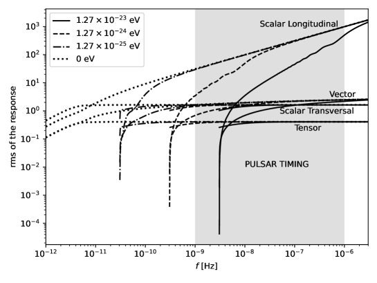
Figure 1: We show the rms of the Pulsar Timing response for all the gauge-invariant variables of the polarization modes. For all cases, we have used the massive dispersion relation $\eta_{A}(f)=\sqrt{1-(m_{A}/2\pi f)^{2}}$. The shaded region indicates the frequency range of the Pulsar Timing technique. Notice that if the mass is about that of the upper bound of the LIGO detector ($1.27\times 10^{-23}~{}{\rm eV}$) we have remarkable effects in this range.

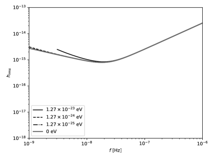
(a) Tensor

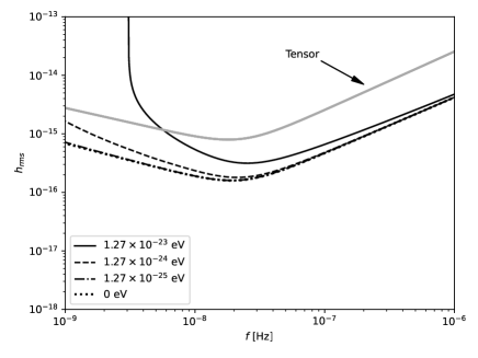
(b) Vector

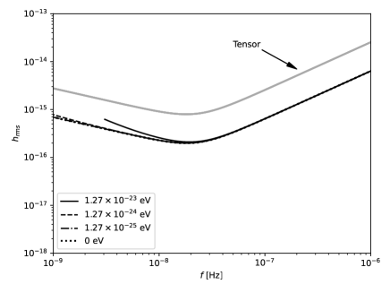
(c) Scalar transversal

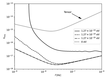
(d) Scalar longitudinal

Figure 2: Sensitivity curves for each gauge-invariant variable of the polarization modes considering the effect of the dispersion relation of massive GWs. The sensitivity to the massless tensor mode is shown in all figures (gray curve). Notice that as the mass approaches the upper bound of the LIGO detector ($1.27\times 10^{-23}~{}{\rm eV}$) we have remarkable effects in the sensitivity. The evidence of a cutoff frequency or even the evidence that such a cutoff is not on the Pulsar Timing frequency band can lead to a more stringent bound of the effective mass of the graviton than that presented by ground-based interferometers.

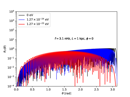
(a) Tensor

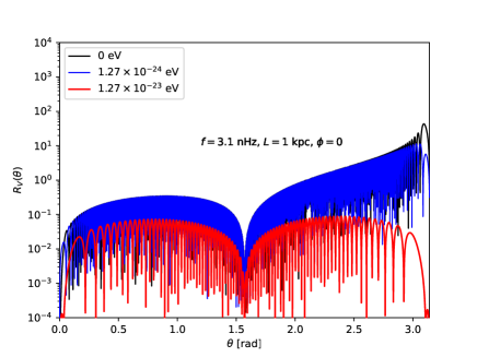
(b) Vector

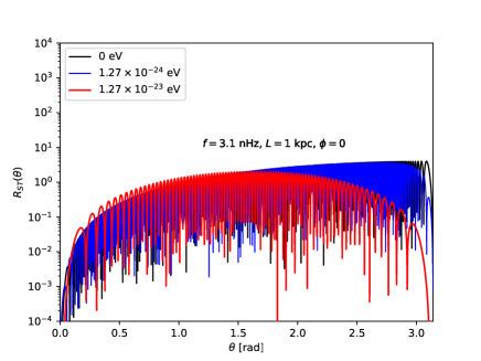
(c) Scalar transversal

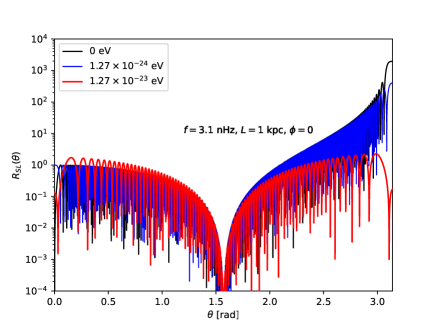
(d) Scalar longitudinal

Figure 3: The Pulsar Timing angular response for the tensor, vector, scalar transversal and scalar longitudinal polarization modes using a massive dispersion relation $\eta_{A}(f)=\sqrt{1-(m_{A}/2\pi f)^{2}}$ for each case. We have considered a typical distance of $L=1$ kpc and an angle $\phi=0$.

Notice that we have not considered any specific form for the dispersion relation so far. Therefore, the analytical expression for the response (104) is a completely general result. In order to evaluate the effect of the dispersion relation on the GW response, henceforth we consider that each mode $A$ has an effective mass $m_{A}$ which results in $\eta_{A}(f)=\sqrt{1-(m_{A}/2\pi f)^{2}}$. In Fig. 1 we show the Pulsar Timing rms response for the scalar longitudinal, scalar transversal, vector, and tensor polarization modes for a typical distance $L=1~{}{\rm kpc}$.

Finally, we define the sensitivity by $\sqrt{S_{y}(f)B}/R^{\rm rms}_{A}$, where $S_{y}(f)$ is the noise spectrum affecting the relative frequency shift of Pulsar Timing and $B$ is the bandwidth corresponding to an integration time of 10 years ($B=1{\rm cycle}/10~{}{\rm years}$). Our estimated sensitivity is based on the noise model discussed in [39] for which $S_{y}(f)$ is given by

$$S_{y}(f)=[4.0\times 10^{-31}f^{-1}+3.41\times 10^{-8}f^{2}]{\rm Hz}^{-1}.$$ (106)

The resulting Pulsar Timing sensitivities to the polarization states are shown in Fig. 2. Notice that the sensitivity to the scalar longitudinal mode is some orders of magnitude better than the sensitivities of other polarizations, and the sensitivity to the vector modes can be up to five times better than that of the tensor mode. The response decreases as the wavelength of the GWs is of the order or larger than the distance from Earth to the Pulsar (long-wavelength limit). If $m_{A}=0$ this happens in a very small frequency, far beyond the Pulsar Timing frequency band $(10^{-9}-10^{-6}~{}{\rm Hz})$ (see Fig. 1). On the other hand, for a non-null mass, a fast decrease in the response can occur in this band as the technique approaches the long-wavelength limit. The cutoff frequency for which the response vanishes is related to the mass by

$$f_{c}=\left(\frac{m}{m_{\rm up}}\right)3.07\times 10^{-9}~{}{\rm Hz},$$ (107)

where we have considered the upper bound on the graviton mass imposed by LIGO, $m_{\rm up}=1.27\times 10^{-23}~{}{\rm eV}/c^{2}$ [3], as a fiducial mass. Obviously, the effective mass of the vector and scalar polarizations do not need to respect this upper bound since it was derived from detections of the tensor modes.

In Fig. 3 we show, as an example, the angular response (i.e., the frequency-dependent antenna pattern) given by Eqs. (96), (97), (102) and (103) at the frequency $f=3.1~{}{\rm nHz}$ and $\phi=0$ considering a single Pulsar. Depending on the value of the mass $m$, we can have the long-wavelength regime at this frequency or not.

When the GW approaches the long-wavelength regime, the symmetry of the response around $\theta=\pi/2$ is restored for all the polarization modes. This case is shown in red in Fig. 3 for each polarization. The behavior of the response, in this case, is similar to that of ground-based interferometers. At $\theta=\pi/2$ the tensor polarization has the maximum response and the response vanishes for the scalar longitudinal and vector modes. On the other hand, the response for the scalar transversal mode is identical in form to the response for tensor polarization. In the same figure, we notice the oscillations in the response which comes from the square brackets in the Eqs. (96), (97), (102) and (103). In the present case, the angles for which this term vanishes for a given frequency $f$ are given by

$$\cos\theta_{n}=\frac{1}{\eta_{A}}\left(\frac{n}{fL}-1\right),~{}~{}n=0,1,2,\dots$$ (108)

As we mentioned earlier, for the massless case the Pulsar Timing is out of the long-wavelength regime for the entire frequency range. In this case, we can notice an asymmetry of the response of GWs propagating in the parallel directions of the electromagnetic signal ($\pi/2<\theta<\pi$) with respect to GWs propagating in the antiparallel directions ($0<\theta<\pi/2$). For GWs traveling in parallel directions, the response can be some orders of magnitude higher than those traveling in antiparallel directions. This effect occurs for tensor, vector, and scalar modes. However, for the scalar longitudinal and vector modes, one can notice a remarkable enhancement of the response. This enhancement effect has been noticed for the first time by the present author and a collaborator [37, 38]. It is associated with the longitudinal behavior of the mentioned polarization modes and with the relative direction of the GW wave vector $\vec{k}$ with respect to the direction of propagation of the electromagnetic signal emitted by the Pulsar.

In the present scope, the physical origin of the enhancement effect in the response of longitudinal polarizations can be understood in light of Eq. (87). First of all, remember that in this case, the Riemann curvature tensor has components not only transverse to the direction of the propagation of the GW, but also in the longitudinal direction. Since the Riemann tensor is a function of the retarded time $u$, and $u$ depends on $\theta$, light rays coming from different directions ‘see’ the curvature generated by the GW differently. Consider that we are out of the long-wavelength regime. The light rays traveling in the opposite directions of the GWs pass through several maxima and minima of the curvature changing continuously its frequency. Since the final frequency shift measured at Earth is an integrated effect of the curvature, the result can be zero for some directions. On the other hand, those light rays propagating parallel or almost parallel to the GW experience fewer oscillations of the curvature. In this case, the final effect can be a higher frequency shift when compared with the anti-parallel case. This is because the average curvature is higher generating an increase in the response as $\theta\rightarrow\pi$. When one approaches the long-wavelength regime, the light signals coming from different directions experience fewer curvature oscillations and the final effect in the frequency shift becomes symmetric. Finally, in the long-wavelength regime, the oscillations of the curvature cannot be noticed at all in a one-way light travel. In this situation, we have the usual frequency-independent antenna patterns of ground-based interferometers.

The same argument applies to the explanation of the asymmetry of the transversal polarizations (scalar transversal and tensor) out of the long-wavelength regime. But in this case, the curvature goes to zero as one approaches $\theta=0$ or $\theta=\pi$ resulting in a suppression of the enhancement effect for $\theta\rightarrow\pi$.

In the Fig. 2, we notice that the graviton mass has a remarkable effect on the sensitivity curves as it approaches the upper bound of the LIGO detector ($1.27\times 10^{-23}~{}{\rm eV}$). For tensor and scalar transversal polarizations, the main effect is a limit in the sensitivity established by the cutoff frequency $f_{c}$ given by the relation (107). On the other hand, for vector and scalar longitudinal polarization modes, we have a significant change in the shape of the sensitivity curve including a change in the frequency of maximum sensitivity. The sensitivity curves for massive gravitons are indistinguishable from that of the massless case if the effective mass is two orders of magnitude smaller than that of the LIGO upper bound in the case of vector and scalar longitudinal polarizations. Whereas for the transversal polarizations, it is enough that the graviton mass is one order of magnitude smaller than $m_{\rm up}$. Remember that $m_{\rm up}$ was obtained from observations of the tensor mode. This means that, in principle, the effective mass of the vector and scalar polarizations can be greater than $m_{\rm up}$. If $m$ is about three orders of magnitude higher than $m_{\rm up}$ these polarizations would be undetectable in the Pulsar Timing frequency band.

5 Conclusion

We have shown that the Bardeen framework enables a clear description of the six polarization modes of GWs even if each mode has a general dispersion relation. The response given by Eq. (4) shows an explicit relation between a physical observable (the derivative of the frequency shift) with the gauge-invariant variables. Therefore, this relation means we have a bridge between theory and experiment, avoiding possible ambiguities of gauge choice. A new gauge-invariant variable was introduced [see Eq. (33)] aiming for an unambiguous description of the scalar longitudinal polarization mode.

In the case of a single Pulsar Timing, we obtained an analytical formula for the rms response [see Eq. (104)] which is valid for any dispersion relation. In the case of a dispersion relation of a massive particle, we have seen that it has a significant impact on the Pulsar Timing sensitivity to scalar longitudinal and vector GWs. Remarkably, the effects of the mass on the Pulsar Timing sensitivity are particularly noticeable if it is of the order of the LIGO’s upper bound for the graviton mass ($m_{\rm up}$). If the mass is two orders of magnitude smaller than $m_{\rm up}$, the sensitivity curves are indistinguishable from the massless case. On the other hand, in the case of the scalar transversal and the tensor polarization modes, it is enough that the mass is one order of magnitude smaller than $m_{\rm up}$ to disregard its effects on the sensitivity. The main physical effect in these cases is a limitation in the detectability of these modes established by a cutoff frequency that depends on the mass. Notice that the effects on the sensitivity appear in the case of Pulsar Timing because the cutoff frequency we have considered lies in the Pulsar Timing frequency band. But, in principle, the cutoff frequency can be higher than the Pulsar Timing band in the case of vector and scalar polarizations. If this happens, such modes would be undetectable by Pulsar Timing experiments. In other words, the absence of detection does not imply that extra polarization states beyond the tensor polarization do not exist. In the future, we plan to analyze other dispersion relations of GWs appearing in the literature to check their implications on the Pulsar Timing sensitivity.

The detection (or absence of detection) of the polarization modes using the Pulsar Timing technique has decisive implications for alternative theories of gravity. Consider, for instance, the case of the theories studied in Section 3.4 for which the tensor mode is massless and the scalar modes can be massive. Suppose that the scalar mode has a mass of about that of the LIGO upper bound, then for frequencies approaching the cutoff $f_{c}\sim 3\times 10^{-9}$ Hz the sensitivity of the scalar longitudinal polarization becomes worse than that of the tensor modes. Below this frequency, the scalar modes could not be detected (or even be produced!). Therefore, suppose we are looking for GWs only in a frequency band below $f_{c}$, and we detect only tensor polarizations. We could be led to the wrong conclusion that the scalar modes do not exist. On the other hand, if we find evidence of the existence of a cutoff frequency for the scalar modes, but not for the tensor modes, this could corroborate the scalar-tensor theories of gravity or $f(R)$-gravity. Moreover, this would lead to a bound on the mass of the scalar mode.

We have seen that the Pulsar Timing sensitivity to the scalar longitudinal mode is some orders of magnitude better than the sensitivity to tensor modes. However, depending on the theory of gravity this could not be an advantage in terms of detection. In the case of the theories we have analyzed, the amplitude of the scalar longitudinal mode is related to the amplitude of the scalar transversal mode through a factor $(m/\omega)^{2}$ [see Eq. (71)]. Therefore, if $m$ is much smaller than the smallest detectable frequency of Pulsar Timing, the scalar-longitudinal mode can become undetectable. In this situation, one could still detect the scalar transversal mode if it is strong enough. Obviously, these results apply to scalar-tensor theories of gravity and $f(R)$-gravity. For other theories of gravity, the relation between $\Theta$ and $\Phi$ should be analyzed as well as the mechanism of generation of these GW modes.

Finally, the evidence of a cutoff frequency for any polarization or even the evidence that such a cutoff is not in the Pulsar Timing band can lead to a more stringent bound on the graviton mass than that presented by ground-based interferometers. Similarly, Pulsar Timing detection presents a great opportunity to test gravity by imposing bounds on the polarization modes of GWs.

Appendix

Here we give the frequency-dependent quantities which appear in Eq. (104).

For the scalar-longitudinal response

$$a^{SL}_{1} =1,$$ (109)

$$a^{SL}_{2} =-4,$$ (110)

$$a^{SL}_{3} =6,$$ (111)

$$a^{SL}_{4} =-4,$$ (112)

$$a^{SL}_{5} =1.$$ (113)

For the scalar-transversal response

$$a^{ST}_{1} =\left[1-\frac{1}{\eta_{S}^{2}(f)}\right]^{2},$$ (114)

$$a^{ST}_{2} =\frac{4}{\eta_{S}^{2}(f)}\left[1-\frac{1}{\eta_{S}^{2}(f)}\right],$$ (115)

$$a^{ST}_{3} =\frac{2}{\eta_{S}^{2}(f)}\left[\frac{3}{\eta_{S}^{2}(f)}-1\right],$$ (116)

$$a^{ST}_{4} =-\frac{4}{\eta_{S}^{4}(f)},$$ (117)

$$a^{ST}_{5} =\frac{1}{\eta_{S}^{4}(f)}.$$ (118)

For the vector response

$$a^{V}_{1} =\frac{1}{4}\left[1-\frac{1}{\eta_{V}^{2}(f)}\right],$$ (119)

$$a^{V}_{2} =\frac{1}{2}\left[\frac{2}{\eta_{V}^{2}(f)}-1\right],$$ (120)

$$a^{V}_{3} =\frac{1}{4}\left[1-\frac{6}{\eta_{V}^{2}(f)}\right],$$ (121)

$$a^{V}_{4} =\frac{1}{\eta_{V}^{2}(f)},$$ (122)

$$a^{V}_{5} =-\frac{1}{4\eta_{V}^{2}(f)}.$$ (123)

For the tensor response

$$a^{T}_{1} =\frac{1}{16}\left[1-\frac{1}{\eta_{T}^{2}(f)}\right]^{2},$$ (124)

$$a^{T}_{2} =\frac{1}{4\eta_{T}^{2}(f)}\left[1-\frac{1}{\eta_{T}^{2}(f)}\right],$$ (125)

$$a^{T}_{3} =\frac{1}{8\eta_{T}^{2}(f)}\left[\frac{3}{\eta_{T}^{2}(f)}-1\right]$$ (126)

$$a^{T}_{4} =-\frac{1}{4\eta_{T}^{4}(f)},$$ (127)

$$a^{T}_{5} =\frac{1}{16\eta_{T}^{4}(f)}.$$ (128)

References

References

- [1] Abbott B P et al. (LIGO Scientific Collaboration, Virgo Collaboration) 2019 Phys. Rev. D 100 104036 (Preprint arXiv:1903.04467)
- [2] Abbott R et al. (LIGO Scientific Collaboration, Virgo Collaboration) 2021 Phys. Rev. D 103 122002 (Preprint arXiv:2010.14529)
- [3] Abbott R et al. (LIGO Scientific Collaboration, Virgo Colaboration, KAGRA Collaboration) 2022 (Preprint arXiv:2112.06861)
- [4] Eardley D M and Lightman A P 1973 Phys. Rev. D 8 3308
- [5] Eardley D M, Lee D L, Lightman A P, Wagoner R V and Will C M 1973 Phys. Rev. Lett. 30 884
- [6] de Paula W L S, Miranda O D and Marinho R M 2004 Class. Quantum Gravity 21 4595
- [7] Alves M E S, Miranda O D and de Araujo J C N 2009 Phys. Lett. B 679 401
- [8] Alves M E S, Miranda O D and de Araujo J C N 2010 Class. Quantum Gravity 27 145010
- [9] Hohmann M 2012 Phys. Rev. D 85 084024
- [10] Myung Y S and Moon T 2014 J. Cosmol. Astropart. Phys. 10 043
- [11] Alves M E S, Moraes P H R S, de Araujo J C N and Malheiro M 2016 Phys. Rev. D 94 024032
- [12] Sharif M and Siddiqa A 2017 Astroph. and Space Science 362 226
- [13] Bertolami O, Gomes C and Lobo F S N 2018 The Europ. Physical Journal C 78 303
- [14] Abedi H and Capozziello S 2018 The Europ. Physical Journal C 78 474
- [15] Mebarki N 2019 Journal of Physics Conference Series (Journal of Physics Conference Series vol 1269) p 012015
- [16] Toniato J D 2019 The Europ. Physical Journal C 79 680
- [17] Wagle P, Saffer A and Yunes N 2019 Phys. Rev. D 100 124007
- [18] Haghshenas M and Azizi T 2020 International Journal of Modern Physics D 29 2050004
- [19] Gogoi D J and Goswami U D 2020 The European Physical Journal C 80 1101
- [20] Liang D, Gong Y, Hou S and Liu Y 2017 Phys. Rev. D 95 104034
- [21] Gong Y and Hou S 2018 Universe 4 85
- [22] Hou S, Gong Y, and Liu Y 2018 The European Physical Journal C 78 378
- [23] Hyun Y H, Kim Y and Lee S 2019 Phys. Rev. D 99 124002
- [24] Bardeen J M 1980 Phys. Rev. D 22 1882
- [25] Mukhanov V F, Feldman H and Brandenberger R H 1992 Phys. Rept. 215 203
- [26] Newman E and Penrose R 1962 J. Math. Phys. 3 566
- [27] Newman E and Penrose R 1962 J. Math. Phys. 4 998
- [28] Will C M 2018 Theory and Experiment in Gravitational Physics (Cambridge University Press)
- [29] Jaccard M, Maggiore M and Mitsou E 2013 Phys. Rev D 87 044017
- [30] Wagoner R 1970 Phys. Rev. D 1 3209
- [31] Bergmann P 1968 Int. J. Theor. Phys. 1 25
- [32] Horndeski G 1974 Int. J. Theor. Phys. 10 363
- [33] De Felice A and Tsujikawa S 2010 Living Rev. Relativity 13 3 URL http://www.livingreviews.org/lrr-2010-3
- [34] Yang L, Li C C and Geng C Q 2011 JCAP 08 029
- [35] Koop M J and Finn L S 2014 Phys. Rev. D 90 062002
- [36] Błaut A 2019 Class. Quantum Gravity 36 055004
- [37] Tinto M and Alves M E S 2010 Phys. Rev D 82 122003
- [38] Alves M E S and Tinto M 2011 Phys. Rev D 83 123529
- [39] Jenet F, Armstrong J and Tinto M 2011 Phys. Rev D 83 081301