The structural invariants
of Goursat distributions

Abstract.

This is the first of a pair of papers devoted to the local invariants of Goursat distributions. The study of these distributions naturally leads to a tower of spaces over an arbitrary surface, called the monster tower, and thence to connections with the topic of singularities of curves on surfaces. Here we study those invariants of Goursat distributions akin to those of curves on surfaces, which we call structural invariants. In the subsequent paper we will relate these structural invariants to the small-growth invariants.

1. Introduction

This is the first of a pair of papers devoted to the local invariants of Goursat distributions. A distribution $D$ on a smooth manifold $M$ is a subbundle of the tangent bundle $TM$. It is called Goursat if the Lie square sequence

$$D=D_{1}\subset D_{2}\subset D_{3}\subset\cdots$$

(as defined in Section 2) is a sequence of vector bundles for which

$$\operatorname{rank}D_{i+1}=1+\operatorname{rank}D_{i}$$

until one reaches the full tangent bundle. As realized by Montgomery and Zhitomirski [17], the study of Goursat distributions naturally leads to a tower of spaces over an arbitrary surface, called the monster tower, and thence to connections with the topic of singularities of curves on surfaces. In the local study of such curves and in the local study of Goursat distributions, an important role is played by invariants: for curves on surfaces there are many well-studied invariants, such as those listed on page 85 of [22], whereas for Goursat distributions we have notions related to the analysis of the small growth sequence (which we define in Section 15).

The aims of this pair of papers, taken together, are

1. To give a systematic account of those invariants of Goursat distributions akin to those of curves on surfaces, including the Puiseux characteristic — we call them structural invariants;

2. To explain how they lead to the standard invariants of the small growth sequence: the small growth vector, Jean’s beta vector ([12]), and its derived vector;

3. To present effective recursive methods for calculation.

This paper is devoted to aim 1 and the subsequent paper to aim 2 ; our third aim is addressed throughout both. Our analysis uses the monster tower, which ties together the notions of prolonging a Goursat distribution and lifting a curve. Our starting point is the RVT codes, which provide a way of assigning a code word to each germ of a Goursat distribution and to each irreducible curve germ. Furthermore, our analysis is recursive. In fact, there are two compatible notions of recursion in play, which we call front-end and back-end recursions.

Since we use the monster tower, our account of invariants of curves on surfaces is based on the idea of Nash modifications. Specialists in singularity theory tend to be more familiar with the theory of point blowups. (Intuitively, Nash modification uses tangent lines, whereas ordinary blowing-up uses secant lines.) Most of our basic definitions and all of our structural invariants can be interpreted in the alternative framework of embedded blowups; Section 11 briefly explores this approach. We have tried to give a relatively self-contained exposition, and thus we sometimes offer our own versions of proofs already found elsewhere, especially in [17]. We do this, in part, so as to provide convenient references for our subsequent paper. Our other chief references are [18], [19], and [22].

Figure 1 shows the invariants we will analyze in the two papers; we will also explain the relationships indicated by the arrows. Figure 2 presents an example, using the same layout.

Figure 1. The invariants listed in the top three boxes are invariants of points on monster spaces (as defined in Section 5) and of focal curve germs (as defined in Section 7), akin to invariants of curves on surfaces; the “Goursat” and “restricted” invariants are invariants of germs of Goursat distributions. The invariants listed in the bottom box are invariants of the small growth sequence of a Goursat germ.

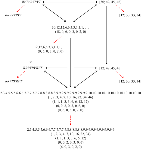
Figure 2. An example of the invariants of Figure 1. The dashed arrows indicate compatible front-end recursions.

Section 2 recalls the basic definitions of Goursat distributions, and Section 3 explains how their basic structural theory leads to code words in the alphabet $R$, $V$, $T$. Section 4 reviews the notion of prolongation, while clarifying a ubitiquous construction in differential geometry which seems never to have been baptized; we coin the term extension. Section 5 introduces the monster tower, while Section 6, following [17], explicates how it is universal for Goursat distributions. Section 7 explains the terminology of focal curve germs. Section 8 explains how one naturally introduces coordinates on the spaces of the monster tower. Section 9 gives the basic stratification theory of divisors at infinity and their prolongations, while Section 10 uses this theory to enlarge the scope of the theory of code words. The brief Section 11 is something of a digression: it explores how several of the notions of the prior sections can be interpreted using embedded resolution via point blowups. With Section 12, we begin to look at the structural invariants; this section is devoted to the Puiseux characteristic, while the subsequent Sections 13 and 14 handle the multiplicity sequence and the vertical orders vector (again a new coinage). The final Section 15 is a brief introduction to the small growth sequence, whose invariants will be the subject of our subsequent paper.

We thank Richard Montgomery, Piotr Mormul, Lee McEwan, Justin Lake, Tom Ivey, and Fran Presas for valuable discussions.

2. Goursat distributions

We begin with a smooth manifold $M$ of dimension $m\geq 2$. Let $D$ be a distribution on $M$, i.e., a subbundle of its tangent bundle $TM$. Let ${\mathcal{E}}$ be its sheaf of sections, which is a subsheaf of the sheaf $\Theta_{M}$ of sections of $TM$. In other words, let $\Theta_{M}$ be the sheaf of vector fields on $M$, and let ${\mathcal{E}}$ be the subsheaf of vector fields tangent to $D$.

The Lie square of ${\mathcal{E}}$ is

$${\mathcal{E}}_{2}=[{\mathcal{E}},{\mathcal{E}}]+{\mathcal{E}},$$

meaning the subsheaf of $\Theta_{M}$ whose sections are generated by Lie brackets of sections of ${\mathcal{E}}$ and the sections of ${\mathcal{E}}$ itself. Note that in general the rank of ${\mathcal{E}}_{2}$ may vary from point to point. If, however, ${\mathcal{E}}_{2}$ is the sheaf of sections of a distribution $D_{2}$, then this rank is constant. Beginning with ${\mathcal{E}}_{1}={\mathcal{E}}$, recursively we define ${\mathcal{E}}_{i+1}$ to be the Lie square of ${\mathcal{E}}_{i}$, and we call

$${\mathcal{E}}_{1}\subseteq{\mathcal{E}}_{2}\subseteq{\mathcal{E}}_{3}\subseteq\cdots$$ (2.1)

the Lie square sequence.

Let $d$ be the rank of $D$. We say that $D$ is a Goursat distribution if each sheaf ${\mathcal{E}}_{i}$ is the sheaf of sections of a distribution $D_{i}$ and if

$$\operatorname{rank}D_{i+1}=1+\operatorname{rank}D_{i}$$

for $i=1,\dots,m-d$. In particular $D_{m-d+1}$ is the tangent bundle $TM$. For a Goursat distribution, the sequence

$$D=D_{1}\subset D_{2}\subset D_{3}\subset\cdots\subset D_{m-d}\subset D_{m-d+1}=TM$$

is also called the Lie square sequence. Since a distribution of rank 1 is always integrable, a Goursat distribution necessarily has rank at least 2.

In the literature on Goursat distributions, it is generally assumed that the corank $m-d$ is at least 2. We find it more convenient to allow these trivial cases:

• $D=TM$,

• $D$ has corank 1, and its Lie square is $TM$,

and call all other cases nontrivial.

Since we are interested in local invariants, we will work with germs of distributions. A Goursat germ consists of a Goursat distribution $D$ on a manifold $M$ and a point $p\in M$; if necessary for our constructions we will replace $M$ by a neighborhood of $p$, and this will not change our invariants. We say that the germ is located at $p$.

3. Code words of Goursat germs

Fix a Goursat germ $D$ at the point $p\in M$. Let $d\geq 2$ be the rank of $D$ and let $m\geq d$ be the dimension of $M$. We give here a self-contained account of how one defines the Goursat code word of $D$ at $p$; this is a word of length $m-d$ in the symbols $R$, $V$, and $T$, which stand for regular, vertical, and tangent. (In the literature on Goursat distributions, these may be called RVT code words, but we prefer to reserve that usage for the slightly more general code words defined in Section 10.) Our account draws upon four sources: Section 9.1 of [14] lays out the basic structural possibilities for Goursat germs; [19] uses these possibilities to attach a code word (using $G$ rather than $R$ and $S$ rather than $V$), invoking the Sandwich Diagram from [17]; the monograph [18] introduces the now-standard notation.

For a distribution $D$, let ${\mathcal{L}}(D)$ denote its Cauchy characteristic. This is the sheaf of vector fields $v$ in $D$ that preserve $D$, meaning that $[v,D]\subset D$. If ${\mathcal{L}}(D)$ is of constant rank, then it is a subdistribution of $D$, and we mildly abuse notation by writing ${\mathcal{L}}(D)$ for both the distribution and its sheaf of sections.

Lemma 1 (Sandwich Lemma of [17]).

For a nontrivial Goursat distribution $D$, its Cauchy characteristic has constant rank and is therefore the sheaf of sections of a subdistribution. We have

$${\mathcal{L}}(D)\subset{\mathcal{L}}(D_{2})\subset D$$

and both inclusions are of corank one.

Proof.

We begin with some remarks on a skew-symmetric bilinear form $\omega$ on a finite-dimensional vector space $V$. We say that a subspace $W$ is isotropic if the restriction of $\omega$ to $W$ is trivial. (Surprisingly, this is not fully standard terminology; it is found, however, in [13, Definition 1.2.4].) By the classification theory of such forms, as found in [10, Section 10.3] or [3, Section 1.1], one infers that if there is an isotropic subspace $W$ of codimension one and if $\omega$ is nontrivial, then the kernel of $\omega$ has codimension one in $W$.

Consider the map

$$D_{2}\times D_{2}\to D_{3}/D_{2}$$

obtained by composing the Lie bracket with the quotient map. Choose a local basis of sections for $D_{2}$ and restrict this map to the fibers at a point $p$:

$$D_{2}(p)\times D_{2}(p)\to D_{3}/D_{2}(p)$$ (3.1)

Since $D_{3}/D_{2}(p)$ is one-dimensional, this is a skew-symmetric bilinear form. The subspace $D(p)$ is isotropic and of codimension one inside $D_{2}(p)$; thus the kernel ${\mathcal{L}}(D_{2})(p)$ of (3.1) has codimension one inside $D(p)$.

Similarly consider the skew-symmetric bilinear form

$$D(p)\times D(p)\to D_{2}/D(p)$$ (3.2)

and observe that the subspace ${\mathcal{L}}(D_{2})(p)$ is isotropic and of codimension one inside $D(p)$; thus the kernel ${\mathcal{L}}(D)(p)$ of (3.2) has codimension one inside ${\mathcal{L}}(D_{2})(p)$. ∎

The Sandwich Lemma can be applied to every nontrivial member of the Lie square sequence of a Goursat distribution to yield the following diagram, in which each inclusion has corank one.

$$\begin{array}[]{ccccccccccccc}&&D=D_{1}&\!\!\!\!\subset\!\!\!\!&D_{2}&\!\!\!\!\subset\!\!\!\!&\!\!\cdots\!\!&\!\!\!\!\subset\!\!\!\!&D_{m-d-1}&\!\!\!\!\subset\!\!\!\!&D_{m-d}&\!\!\!\!\subset\!\!\!\!&TM\\[10.0pt] &&\cup&&\cup&&&&\cup&&&\\[10.0pt] {\mathcal{L}}(D_{1})&\!\!\!\!\subset\!\!\!\!&{\mathcal{L}}(D_{2})&\!\!\!\!\subset\!\!\!\!&{\mathcal{L}}(D_{3})&\!\!\!\!\subset\!\!\!\!&\!\!\cdots\!\!&\!\!\!\!\subset\!\!\!\!&{\mathcal{L}}(D_{m-d})&\end{array}$$ (3.3)

By the Jacobi identity, each ${\mathcal{L}}(D_{i})$ is involutive, so the Frobenius theorem shows that it induces a foliation, called a characteristic foliation.

To define the Goursat code word, we associate a symbol with each square

$$\begin{array}[]{cccc}D_{i}&\!\!\!\!\subset\!\!\!\!&D_{i+1}\\[10.0pt] \ \ \cup&&\cup\\[10.0pt] {\mathcal{L}}(D_{i+1})&\!\!\!\!\subset\!\!\!\!&{\mathcal{L}}(D_{i+2})&\end{array}$$ (3.4)

of diagram (3.3) and then read off the word from right to left. We also associate the symbol $R$ with each of the two incomplete squares at the right end, so that each Goursat code word begins with $RR$. Thus the symbol associated with the square of (3.4) will be the symbol of the code word in position $m-d-i+1$.

To begin, looking at the fibers of our sheaves at $p$, we remark that we know two natural fillings $W$ for the sandwich

$${\mathcal{L}}(D_{i+1})(p)\subset W\subset D_{i+1}(p),$$

since we could use either the hyperplane $W=D_{i}(p)$ or the hyperplane $W={\mathcal{L}}(D_{i+2})(p)$. If the two fillings coincide, that is, if $D_{i}(p)={\mathcal{L}}(D_{i+2})(p)$, then we say that $D_{i}$ is singular at $p$, and we associate the letter $V$ with the square. To continue, we find it convenient to introduce coordinates.

Lemma 2.

Suppose that $D$ is a nontrivial Goursat germ on $M$ at $p$. Consider these sheaves:

$$\begin{array}[]{ccccc}&&D&\!\!\!\!\subset\!\!\!\!&\phantom{D}D_{2}\\[10.0pt] &&\cup&&\\[10.0pt] {\mathcal{L}}(D)&\subset&{\mathcal{L}}(D_{2})&&\end{array}$$

1. There is an ordered pair of coordinate functions $x$ and $y$, part of a system of local coordinates, for which the sheaf ${\mathcal{L}}(D_{2})$ is defined inside $D_{2}$ by $dx=dy=0$.

2. For any such pair of coordinates, either there is a third coordinate $y^{\prime}$ and a constant $C$ so that $D$ is defined inside $D_{2}$ by $dy=(C+y^{\prime})dx$ (we call this the ordinary situation) or there is a third coordinate $x^{\prime}$ so that $D$ is defined inside $D_{2}$ by $dx=x^{\prime}dy$ (we call this the inverted situation).

3. In the ordinary situation, the sheaf ${\mathcal{L}}(D)$ is defined inside $D_{2}$ by $dx=dy=dy^{\prime}=0$, and in the inverted situation by $dx=dy=dx^{\prime}=0$.

Observe that if we reverse the order of $x$ and $y$, the inverted situation becomes the ordinary situation with constant 0. In the ordinary situation, the following diagram shows the equations described in the lemma. These are equations defining the sheaves inside $D_{2}$; thus of course the box at top right is empty.

$$\begin{array}[]{cccccc}&&\boxed{dy=(C+y^{\prime})dx}&\!\!\!\!\subset\!\!\!\!&\boxed{\phantom{XXX}}\\[10.0pt] &&\cup\\ \boxed{\begin{array}[]{c}dx=0\\ dy=0\\ dy^{\prime}=0\end{array}}&\!\!\!\!\subset\!\!\!\!&\boxed{\begin{array}[]{c}dx=0\\ dy=0\end{array}}&\end{array}$$ (3.5)

Proof.

As we have remarked, the distribution ${\mathcal{L}}(D_{2})$ is involutive and thus comes from a foliation. Since ${\mathcal{L}}(D_{2})$ is of corank 2 in $D_{2}$, there must be local coordinates $x$ and $y$ for which ${\mathcal{L}}(D_{2})$ is defined inside $D_{2}$ by the vanishing of $dx$ and $dy$. Since $D$ is of corank one inside $D_{2}$, at every point we have a single dependence between $dx$ and $dy$: we must have $dy=(C+y^{\prime})dx$ in some neighborhood of $p$ for some coordinate function $y^{\prime}$, or $dx=x^{\prime}dy$ for some coordinate function $x^{\prime}$. (The possibilities form a projective line, and the last possibility accounts for the point at infinity.)

One finds that the differential ideal of $\mathcal{L}(D)$ is generated by $dx$, $dy$, and $dy^{\prime}$ in the ordinary situation, and by $dx$, $dy$, and $dx^{\prime}$ in the inverted situation. This can be computed directly, but also appears in [17, p. 463], and follows from the Retraction Theorem for exterior differential systems ([11, Proposition 6.1.17] or [1, Theorem 1.3] or [21, Theorem 5.4]). ∎

We return to the definition of the Goursat code word, by probing further the case where $D_{i}$ is singular at $p$. Considering the square of (3.4), we claim that there are local coordinates so that the sheaves of that diagram are defined inside $D_{i+2}$ by the corresponding equations shown here:

$$\begin{array}[]{cccc}\boxed{\begin{array}[]{c}dy=(C+y^{\prime})dx\\ dx=x^{\prime}dy^{\prime}\end{array}}&\!\!\!\!\subset\!\!\!\!&\boxed{dy=(C+y^{\prime})dx}\\[10.0pt] \ \ \cup&&\cup\\ \boxed{\begin{array}[]{c}dx=0\\ dy=0\\ dy^{\prime}=0\end{array}}&\!\!\!\!\subset\!\!\!\!&\boxed{\begin{array}[]{c}dx=0\\ dy=0\end{array}}&\end{array}$$

Indeed, since we are not concerned with the ordering of $x$ and $y$, we can assume that in the square that would appear just to the right we are in the ordinary situation. Thus, except for the box at top left, our claim is immediate from Lemma 2 applied to $D_{i+2}$. If we now consider the equations of these sheaves inside $D_{i+1}$, then the equations at the bottom left reduce to $dx=dy^{\prime}=0$. Thus $x$ and $y^{\prime}$ are appropriate coordinates for which we can apply part 2 of Lemma 2. Among the possibilities given, the only one for which $D_{i}$ is singular at $p$ is the inverted situation: $dx=x^{\prime}dy^{\prime}$.

Furthermore we see that locally the locus on $M$ on which $D_{i}$ is singular is $x^{\prime}=0$, a nonsingular hypersurface; we denote it by $N(V)$. We now consider the square of (3.4) together with the square to its left:

$$\begin{array}[]{cccccc}D_{i-1}&\!\!\!\!\subset\!\!\!\!&D_{i}&\!\!\!\!\subset\!\!\!\!&D_{i+1}\\[10.0pt] \ \ \cup&&\cup&&\cup\\[10.0pt] {\mathcal{L}}(D_{i})&\!\!\!\!\subset\!\!\!\!&{\mathcal{L}}(D_{i+1})&\!\!\!\!\subset\!\!\!\!&{\mathcal{L}}(D_{i+2})&\end{array}$$ (3.6)

Restricting our attention to $N(V)$, we consider the intersection of its tangent sheaf $\Theta_{N(V)}$ with $D_{i}$. This is of corank one inside $D_{i}$, and is cut out by the additional equation $dx^{\prime}=0$. If the fibers at $p$ of $D_{i-1}$ and $\Theta_{N(V)}\cap D_{i}$ are the same, then we assign the letter $T$ to the square on the left.

Assuming that we have assigned $T$ to this square, we claim that the equations defining the sheaves of diagram 3.6 inside $D_{i+2}$ are as follows:

$$\begin{array}[]{cccccc}\boxed{\begin{array}[]{c}dy=(C+y^{\prime})dx\\ dx=x^{\prime}dy^{\prime}\\ dx^{\prime}=x^{\prime\prime}dy^{\prime}\end{array}}&\!\!\!\!\subset\!\!\!\!&\boxed{\begin{array}[]{c}dy=(C+y^{\prime})dx\\ dx=x^{\prime}dy^{\prime}\end{array}}&\!\!\!\!\subset\!\!\!\!&\boxed{dy=(C+y^{\prime})dx}\\[10.0pt] \ \ \cup&&\cup&&\cup\\ \boxed{\begin{array}[]{c}dx=0\\ dy=0\\ dy^{\prime}=0\\ dx^{\prime}=0\end{array}}&\!\!\!\!\subset\!\!\!\!&\boxed{\begin{array}[]{c}dx=0\\ dy=0\\ dy^{\prime}=0\end{array}}&\!\!\!\!\subset\!\!\!\!&\boxed{\begin{array}[]{c}dx=0\\ dy=0\end{array}}&\end{array}$$

To obtain the equations in the bottom left box, we apply part 3 of Lemma 2, using $D=D_{i+1}$. This tells us that ${\mathcal{L}}(D_{i})$ is defined inside $D_{i+1}$ by $dx=dy^{\prime}=dx^{\prime}=0$; adjoining the equation $dy=(C+y^{\prime})dx=0$ of $D_{i+1}$ inside $D_{i+2}$ and simplifying, we obtain the four indicated equations. To obtain the equations in the top left box, we apply part 2 of Lemma 2 using $D=D_{i}$, Since we have assigned $T$ to the left square, we are in the ordinary situation with constant $C=0$; thus $dx^{\prime}=x^{\prime\prime}dy^{\prime}$ should be in our system of equations, together with the two equations cutting out $D_{i-1}$ inside $D_{i+1}$. We remark that the letters $V$ and $T$ are mutually exclusive, since the former requires the inverted situation and the latter the ordinary situation with $C=0$.

Furthermore we see that the locus $N(VT)$ where we have assigned $V$ to the right box and $T$ to the left box is defined inside $N(V)$ by the additional equation $x^{\prime\prime}=0$. Thus it is a nonsingular submanifold of $M$ of codimension two. Restricting our attention to $N(VT)$, we consider the intersection $\Theta_{N(VT)}\cap D_{i-1}$, cut out inside $D_{i-1}$ by the single equation $dx^{\prime\prime}=0$. If the fibers at $p$ of $D_{i-2}$ and $\Theta_{N(VT)}\cap D_{i-1}$ are the same, then we assign the letter $T$ to the next square to the left.

At this point it becomes clear that all arguments can be repeated: the locus $N(VT^{\tau})$ will be a nonsingular submanifold in $M$ of codimension $\tau+1$, with explicit equations $x^{\prime}=x^{\prime\prime}=\cdots=x^{(\tau+1)}=0$; and we will assign yet another $T$ if

$$D_{i-(\tau+1)}(p)=\Theta_{N(VT^{\tau})}\cap D_{i-\tau}(p).$$

Having explained when to associate $V$ or $T$ with a square of diagram (3.3), to finish the definition of the Goursat code word we declare that in all other circumstances we associate the symbol $R$. Thus the possibilities for Goursat code words are circumscribed as follows:

• The first two symbols are $RR$.

• The symbol $T$ may only be used immediately following a $V$ or $T$.

The arguments used to prove Lemma 2 also give an Existential Sandwich Lemma, as follows.

Lemma 3.

Suppose that $D$ is a nontrivial Goursat distribution of rank greater than 2. Any distribution $E$ sandwiched between ${\mathcal{L}}(D)$ and $D$ (i.e., of corank one in $D$ and having ${\mathcal{L}}(D)$ as a corank one subbundle) is Goursat, with Lie square $E_{2}=D$ (i.e., $E$ is a “Lie square root” of $D$). The possibilities for $E$ form a projective line, and the corresponding code word symbol can be any one of the possible symbols, subject to the constraints just mentioned.

4. Prolongation and extension

The work of Montgomery and Zhitomirskii [17, 18] shows that the study of Goursat distributions naturally leads to the construction of a tower of spaces. Unbeknownst to them, the construction had previously been used in algebraic geometry, but had never been connected to Goursat distributions. (This earlier work includes three papers by the first two authors, including [6].)

Once again we work with a smooth manifold $M$ carrying a distribution $D$ of rank $d$. Let $\widetilde{M}=\mathbf{P}D$, the total space of the projectivization of the bundle, and let $\pi:\widetilde{M}\to M$ be the projection. A point $\widetilde{p}$ of $\widetilde{M}$ over $p\in M$ represents a line inside the fiber of $D$ at $p$, and since $D$ is a subbundle of $TM$, this is a tangent direction to $M$ at $p$. Let

$$d\pi:T{\widetilde{M}}\to\pi^{*}TM$$

denote the derivative map of $\pi$. A tangent vector to $\widetilde{M}$ at $\widetilde{p}$ is said to be a focal vector if it is mapped by $d\pi$ to a tangent vector at $p$ in the direction represented by $\widetilde{p}$; in particular a vector mapping to the zero vector (called a vertical vector) is considered to be a focal vector. The subspace of focal vectors is called the focal space. The set of all focal vectors forms a subbundle $\widetilde{D}$ of $T{\widetilde{M}}$, called the prolongation of $D$ or the focal bundle; its rank is again $d$. The vertical vectors form a subbundle, called the vertical bundle or the relative tangent bundle, denoted $T({\widetilde{M}/M})$.

In their Proposition 5.1, Montgomery and Zhitomirskii [17] establish the following fundamental fact: If $D$ is a Goursat distribution of rank 2, then so is $\widetilde{D}$.

To be more precise, we need to clarify a construction in differential geometry which seems to lack a standard terminology or notation. Let $\varphi:N\to M$ be a submersion and let ${\mathcal{F}}$ be a sheaf of vector fields on $M$. The extension of ${\mathcal{F}}$ by $\varphi$, denoted $\varphi^{\bullet}{\mathcal{F}}$, is the sheaf of all vector fields $v$ on open sets of $N$ satisfying the condition

$$d\varphi(v(q))\in{\mathcal{F}}(\varphi(q))$$

at each point $q$ of the open set. If ${\mathcal{F}}$ is the sheaf of sections of a distribution $D$, then $\varphi^{\bullet}{\mathcal{F}}$ is the sheaf of sections of a distribution, which we denote by $\varphi^{\bullet}D$. Note that our definition says $v\in\varphi^{\bullet}{\mathcal{F}}$ if $d\varphi\circ v$ is a section of the usual pullback bundle $\varphi^{*}{\mathcal{F}}$. Thus we are not describing the usual pullback of a bundle, nor is this the usual notion of an inverse image sheaf or a pullback sheaf in algebraic geometry, as described in [9]. It is, however, consistent with the usage of [2] and [17]. These authors use the potentially ambiguous notation $\varphi^{*}$; hence our introduction of new notation and terminology.

Returning to the prolongation construction, we observe that for a distribution $D$ on $M$, we have relations among vector bundles on $\widetilde{M}$ as indicated in the following diagram.

The four bundles on the left are distributions, i.e., subbundles of $T\widetilde{M}$. The ranks of the bundles in the top row are (from left to right) $d-1$, $d$, and 1; the ranks in the bottom row are $d-1$, $2d-1$, and $d$. Here ${\mathcal{O}}_{D}(-1)$ denotes the tautological line bundle.

Suppose that near $p\in M$ we have a set of equations cutting out $D$ inside $TM$. This will be a set of linear equations in the differentials of the local coordinates with coefficients in the local coordinates. At a point $q\in\widetilde{M}$ over $p$ we can use a system of local coordinates including the local coordinates pulled back from $M$; then the very same set of equations cuts out the extension $\pi^{\bullet}D$ inside $T\widetilde{M}$. To give equations for the prolongation $\widetilde{D}$, let us assume for simplicity that $D$ has rank 2. Among our coordinate functions at $p$ we can find a pair $x$ and $y$ such that their differentials $dx$ and $dy$ are independent linear functionals on the fiber of $D$ at $p$. Then $\widetilde{D}$ is cut out inside $\pi^{\bullet}D$ by one additional equation expressing the dependence of $dx$ and $dy$; this will be either $dy=(C+y^{\prime})dx$ (for a suitable local coordinate $y^{\prime}$) or $dx=x^{\prime}dy$ (for a suitable local coordinate $x^{\prime}$).

Returning to the situation of Montgomery and Zhitomirskii’s Proposition 5.1, what they assert is that if

$$D\subset D_{2}\subset D_{3}\subset\cdots$$

is the Lie square sequence of a Goursat distribution $D$ of rank 2, then

$$\widetilde{D}\subset\pi^{\bullet}D\subset\pi^{\bullet}D_{2}\subset\pi^{\bullet}D_{3}\subset\cdots$$

is the Lie square sequence of $\widetilde{D}$, which is again Goursat of rank 2. The assertion is clear from the general properties of extension, except for the claim that $\widetilde{D}$ is Goursat. To see this, one simply remarks that the relative tangent bundle $T({\widetilde{M}/M})$ is an involutive subbundle of $\pi^{\bullet}D$ of corank 2, and thus must be ${\mathcal{L}}(D)$; then Lemma 3 shows that $\widetilde{D}$ is Goursat with Lie square $\pi^{\bullet}D$. Note that

$$\widetilde{D}_{2}=\pi^{\bullet}D$$ (4.1)

and more generally that $\widetilde{D}_{i+1}=\pi^{\bullet}D_{i}$.

Now observe that the general prolongation construction, when applied to a manifold $M$ carrying a distribution $D$ of rank $d$, yields a new manifold $\widetilde{M}$ carrying a new distribution $\widetilde{D}$. Thus we can iterate this construction to obtain an infinite tower of spaces and submersions

$$\cdots\to\widetilde{\widetilde{M}}\to\widetilde{M}\to M$$ (4.2)

together with their associated focal bundles.

We consider a curve $C$ on $M$ which has a nontrivial smooth parameterization; henceforth we will just say “curve.” Suppose that $p$ is a nonsingular point on $C$. If at $p$ the tangent vector of $C$ is contained in the fiber of $D$, we say $C$ is tangent to $D$ at $p$. We say that $C$ is a focal curve if it is tangent to $D$ at each nonsingular point. We can associate with $p$ the point of $\widetilde{D}$ representing the tangent direction of $C$ at $p$. Thus, away from singularities, we have a curve $\widetilde{C}$ in $\widetilde{M}$, the lift of $C$. We also want to associate a point (or perhaps several points) of $\widetilde{M}$ with a singular point of $C$, and we do so by fiat: we lift at all nonsingular points of $C$, and then take the closure. Intuitively, we are associating to a singular point all the possible limiting tangent directions. We observe that the lift of a focal curve on $M$ gives us a focal curve on $\widetilde{M}$, i.e., the lift of such a curve will be tangent to the focal bundle. Thus, if we like, we can iterate the construction by further lifting.

5. The monster tower

If we begin by letting $D$ be the tangent bundle $TM$, then the tower of (4.2) is called the monster tower (or Semple tower) over the base manifold $M$. In the tower

$$\cdots\to M(k)\xrightarrow{\pi_{k}}M(k-1)\xrightarrow{\pi_{k-1}}\cdots\to M(2)\xrightarrow{\pi_{2}}M(1)\xrightarrow{\pi_{1}}M$$ (5.1)

we say that $M(k)$ is the monster space at level $k$. As above, we set $m=\text{dim}M\geq 2$. Each space $M(k)$ is a fiber bundle over $M(k-1)$, with fiber a projective space of dimension $m-1$. The focal bundle on $M(k)$ is denoted $\Delta(k)$.

In general this has nothing to do with Goursat distributions. If, however, we begin with a smooth surface $S$, then its tangent bundle is a trivial Goursat distribution of rank 2; thus the focal bundles are likewise rank 2 Goursat distributions. In this case the fibers of the maps in (5.1) are projective lines. The Lie square sequence of the Goursat distribution $\Delta(k)$ is

$$\Delta(k)\subset\Delta(k)_{2}\subset\Delta(k)_{3}\subset\cdots\subset\Delta(k)_{k}\subset\Delta(k)_{k+1}=TS(k).$$

Continuing to assume that the base manifold is a surface $S$, we apply (4.1) to $\pi_{k}$; this tells us that the Lie square of $\Delta(k)$ can be obtained by extension:

$$\Delta(k)_{2}=\pi^{\bullet}_{k}\,\Delta(k-1).$$ (5.2)

More generally, the other bundles in its Lie square sequence are extensions from lower levels:

$$\Delta(k)_{j}=\pi^{\bullet}\Delta(k-j+1),$$ (5.3)

where $\pi:S(k)\to S(k-j+1)$.

If we apply the lifting construction to the monster tower, the lift of a focal curve on $S(k)$ — a curve tangent to $\Delta(k)$ — is a focal curve on $S(k+1)$, and we can iterate the construction to lift upward any desired number of levels in the tower. If in particular we start with a curve $C$ on $S$ (automatically a focal curve) we obtain curves $C(1)$ on $S(1)$, $C(2)$ on $S(2)$, etc.

As we have said, lifting associates with a singular point all the possible limiting tangent directions. For example, if the curve $C$ has a node at $p$, then $C(1)$ will have two points over $p$, and if $C$ has a cusp then it has a single point over $p$, but this will be a nonsingular point on the threefold $C(1)$. In the mathematical literature, $C(1)$ is also called the Nash modification of $C$.

6. Universality of the monster tower

As we previously noted, the monster spaces over a smooth surface $S$ naturally carry Goursat distributions of rank 2. In [17], Montgomery and Zhitomirskii show that these spaces are universal for Goursat distributions of rank 2. More precisely, they show that each nontrivial Goursat germ of rank 2 on a manifold of dimension $m=2+k$ (with $k\geq 2$) is equivalent to the Goursat germ of $\Delta(k)$ at some point of $S(k)$. They prove this by a process which they call deprolongation, which we explicate here, and explain how it leads to the universality. (They also define a deprolongation process for Goursat germs of higher rank, but we do not consider that process here.)

Consider a nontrivial Goursat germ $D$ of rank 2 at the point $p\in M$. Recall that the Cauchy characteristic ${\mathcal{L}}(D_{2})$ induces a characteristic foliation; the leaves are curves. Locally, one can contract these curves, creating a smooth manifold $M/{\mathcal{L}}(D_{2})$, the leaf space, equipped with a submersion $\lambda:M\to M/{\mathcal{L}}(D_{2})$. Since each of the bundles in the Lie square sequence of $D$ contains the bundle ${\mathcal{L}}(D_{2})$, we have a sequence

$$\lambda_{*}(D/{\mathcal{L}}(D_{2}))\subset\lambda_{*}(D_{2}/{\mathcal{L}}(D_{2}))\subset\lambda_{*}(D_{3}/{\mathcal{L}}(D_{2}))\subset\cdots$$ (6.1)

of bundles on $M/{\mathcal{L}}(D_{2})$, with $\operatorname{rank}(\lambda_{*}(D_{j}/{\mathcal{L}}(D_{2}))=\operatorname{rank}(D_{j})-1=j$. Each of these bundles extends to the corresponding bundle in the Lie square sequence of $D$:

$$\lambda^{\bullet}\Bigl{(}\lambda_{*}(D_{j}/{\mathcal{L}}(D_{2}))\Bigl{)}=D_{j}.$$

We claim that if we omit the first bundle $\lambda_{*}(D/{\mathcal{L}}(D_{2}))$ of (6.1) we obtain a Lie square sequence

$$\lambda_{*}(D_{2}/{\mathcal{L}}(D_{2}))\subset\lambda_{*}(D_{3}/{\mathcal{L}}(D_{2}))\subset\cdots.$$ (6.2)

Indeed, for $j\geq 2$ the Cauchy characteristic ${\mathcal{L}}(D_{j})$ contains ${\mathcal{L}}(D_{2})$; thus the Lie square map $D_{j}\times D_{j}\to D_{j+1}$ yields a surjection from $D_{j}/{\mathcal{L}}(D_{2})\times D_{j}/{\mathcal{L}}(D_{2})$ to $D_{j+1}/{\mathcal{L}}(D_{2})$.

Thus $\lambda_{*}(D_{2}/{\mathcal{L}}(D_{2}))$ is a Goursat distribution of rank 2 on the leaf space. We call it the deprolongation of $D$.

Part 1 of Lemma 2 tells us that locally ${\mathcal{L}}(D_{2})$ is defined inside $D_{2}$ by the vanishing of $dx$ and $dy$, where $x$ and $y$ are part of a system of local coordinates. Thus these two functions are constant on the leaves, and descend to functions on the leaf space. Since the total space of ${\mathcal{L}}(D_{2})$ is of codimension 2 inside that of $D_{2}$, the differentials $dx$ and $dy$ remain independent when restricted to $\lambda_{*}(D_{2}/{\mathcal{L}}(D_{2}))$. Part 2 of the same lemma then tells us that locally each point of $p\in M$ can be interpreted as a tangent direction to the point $\lambda(p)$ lying inside $\lambda_{*}(D_{2}/{\mathcal{L}}(D_{2}))$, and that $D$ is the focal bundle. Thus if we apply the prolongation construction to $\lambda_{*}(D_{2}/{\mathcal{L}}(D_{2}))$, we obtain a projective line bundle over the leaf space that contains the neighborhood on $M$ with which we started, and the prolongation of $\lambda_{*}(D_{2}/{\mathcal{L}}(D_{2}))$ is $D$. In this sense, the operations of prolongation and deprolongation are inverses.

Deprolongation can be applied repeatedly. If we begin with a nontrivial Goursat germ $D$ of rank 2 and corank $k\geq 2$, then we can deprolong it $k-1$ times, arriving at a (trivial) Goursat germ of rank 2 and corank 1, i.e., a distribution germ whose Lie square is the tangent bundle of the base threefold. It is well-known that there is just one such distribution (up to equivalence of germs of distributions), the contact distribution: in appropriate local coordinates $x$, $y$, $y^{\prime}$, it is the distribution defined by $dy=y^{\prime}dx$. Thus $D$ is found somewhere in the prolongation tower over this distribution, i.e., it is equivalent to the germ of the prolongation of the contact distribution at some point in the $(k-1)$st space in this tower. As the contact distribution is equivalent to $\Delta(1)$ at any point of $S(1)$, this shows that $D$ appears somewhere in the monster tower.

One could actually stop this process one step earlier, arriving at a Goursat germ whose rank and corank are both 2. Again one knows that such a germ is unique: it is the Engel distribution, given in local coordinates $x$, $y$, $y^{\prime}$, $y^{\prime\prime}$ by the vanishing of $dy-y^{\prime}dx$ and $dy^{\prime}-y^{\prime\prime}dx$. See Sections 6.2.2 and 6.11 of [15]. The Engel distribution is equivalent to $\Delta(2)$ at any point of $S(2)$.

Alternatively, one can continue it by one additional step, but this step is different, since it is not dictated by the Cauchy characteristic. Given the germ of the contact distribution, one can deprolong in any direction tangent to this distribution, creating a surface whose tangent bundle will prolong to the contact distribution. We illustrate this by two examples.

Example 4.

The coordinate names $x$, $y$, $y^{\prime}$ naturally suggest that one should contract the curves on which $x$ and $y$ are constant; on the resulting surface with coordinates $x$ and $y$ one interprets $y^{\prime}$ as $dy/dx$.

Example 5.

Alternatively, let $X=y^{\prime}$, let $Y=y-y^{\prime}x$, and let $Y^{\prime}=-x$. (To motivate this, think of $X$ and $Y$ as “slope” and “intercept.”) Since $dY=dy-y^{\prime}dx-xdy^{\prime}$ and $dy-y^{\prime}dx$ vanishes on the contact distribution, we see that in our new coordinates the contact distribution is defined by the equation $dY=Y^{\prime}dX$. Thus one can equally well obtain a surface by contracting the curves on which $X$ and $Y$ are constant, and its tangent bundle will likewise prolong to the contact distribution.

Observe that, given a Goursat germ $D$ of rank 2 and corank $k$, the process we have described for finding a point $p_{k}$ on the monster space $S(k)$ over a surface $S$ is a recursive process. By repeated deprolongation we first construct the surface $S$ and a point $p_{0}$; then by the prolongation construction we build $S(1)$ and a point $p_{1}$ lying over $p_{0}$, then $S(2)$ and $p_{2}$, etc.

What about Goursat distributions of rank greater than two? Given a nontrivial Goursat germ $D$ of rank $d\geq 3$, Lemma 3 can be applied $d-2$ times to obtain the beginning of a Lie square sequence

$$E\subset E_{2}\subset\cdots\subset E_{d-1}=D,$$

where $E$ is a rank 2 Goursat germ. As we have just observed, $E$ can be obtained by repeated prolongation of the (threefold) contact distribution. Letting $j$ and $k$ denote the coranks of $D$ and $E$ respectively, we observe that $k=j+d-2$; thus $j+d-3$ steps of prolongation are required. We conclude that any Goursat germ can be found within the monster tower over a surface.

7. Focal curve germs

Throughout the remainder of the paper, we work in the monster tower over a smooth surface $S$. We will be studying local invariants, and thus we are interested in a focal curve germ consisting of a point $p$ on some monster space $S(k)$, together with a locally irreducible focal curve passing through $p$; if necessary we will replace $S(k)$ by a neighborhood of $p$. We say that the germ is located at $p$ or that $p$ is its location. Note in particular that every irreducible curve germ on $S$ is automatically a focal curve germ.

A focal curve germ on $S(k)$ may project to a single point of $S$. Such a germ is said to be critical. We are using the terminology of Montgomery and Zhitomirskii [18, Definition 2.16], but our definition differs slightly from theirs, since they do not apply the terminology to a curve in $S(1)$. This reflects a difference in viewpoint: they are studying Goursat distributions, whereas we are equally focused on curves as objects of intrinsic interest. One can easily characterize a critical germ: it is either the germ of a fiber of $S(k)$ over $S(k-1)$, or the lift from some lower level of such a germ. A tangent direction to a critical germ is also called critical.

If the focal curve germ $C(k)$ located at $p\in S(k)$ is not critical, then one may project it to the base surface $S$, obtaining a curve germ $C$ there, and then recover $C(k)$ by repeated lifting of $C$. (Note that this justifies the notation $C(k)$.)

We say that $C(k)$ is regular if it is nonsingular and if the tangent direction at $p$ is not critical. Starting with an arbitrary focal curve germ, we can lift it through the tower. If, after a finite number of steps, we obtain a regular focal curve germ, then we say the original germ is regularizable. Its regularization level $r$ is the smallest value for which $C(r)$ is regular. Note that $r\geq k$, with equality if and only if $C(k)$ is regular. If $r>k$, then $C(k+1)$ through $C(r)$ all have regularization level $r$.

A critical germ provides the basic example of a focal curve germ which is not regularizable. There are, however, other non-regularizable germs: one can create a curve germ that agrees with a critical germ to infinite order, i.e., that cannot be separated from the critical germ by any number of liftings. In [18, Theorem 2.36], the authors observe that one way to avoid such curves is to assume that $S$ has an analytic structure; they show that a non-critical analytic curve is regularizable. We will take a slightly different approach, hypothesizing “regularizable” as needed in our later results.

We will give examples of the definitions in the next section, which will introduce natural coordinate charts on the monster spaces.

8. Coordinates on monster spaces

We now explain how to introduce coordinates on the monster spaces over a surface $S$, and relate them to the coordinates previously employed in Lemma 2. Let $x$ and $y$ be coordinates on a neighborhood $U$ in $S$. On $U(k)$ there are $2^{k}$ charts, each of which is a copy of $U\times\mathbf{A}^{k}$, the product of the base neighborhood $U$ and $k$-dimensional affine space, and on each chart there are $k+2$ coordinate functions: the pullback of $x$ and $y$ from $U$, together with $k$ affine coordinates. At each level $j$, by a recursive procedure, two of these coordinates are designated as active coordinates. One is the new coordinate $\mathbf{n}_{j}$, and the other is the retained coordinate $\mathbf{r}_{j}$. In addition, for $j>0$, a third coordinate is designated as the deactivated coordinate $\mathbf{d}_{j}$.

To describe the recursive procedure, we begin with a chart on $U(j)$ with coordinates $\mathbf{n}_{j}$, $\mathbf{r}_{j}$, and $\mathbf{d}_{j}$ together with $j-1$ unnamed coordinates. At each point of the chart, the fiber of $\Delta(j)$ (except for the zero vector) consists of tangent vectors for which either the restriction of the differential $d\mathbf{n}_{j}$ or that of $d\mathbf{r}_{j}$ is nonzero. Create a chart at the next level by choosing one of the following two options:

• Assuming the restriction of $d\mathbf{r}_{j}$ is nonzero, let $\mathbf{n}_{j+1}=d\mathbf{n}_{j}/d\mathbf{r}_{j}$; then set $\mathbf{r}_{j+1}=\mathbf{r}_{j}$ and $\mathbf{d}_{j+1}=\mathbf{n}_{j}$. We call this the ordinary choice.

• Assuming the restriction of $d\mathbf{n}_{j}$ is nonzero, let $\mathbf{n}_{j+1}=d\mathbf{r}_{j}/d\mathbf{n}_{j}$; then set $\mathbf{r}_{j+1}=\mathbf{n}_{j}$ and $\mathbf{d}_{j+1}=\mathbf{r}_{j}$. We call this the inverted choice.

To begin the process we always make an ordinary choice, but there are two possibilities. On $U$ the active coordinates are $x$ and $y$, either of which may be designated as the retained coordinate $\mathbf{r}_{0}$; the other coordinate is $\mathbf{n}_{0}$, and there is no deactivated coordinate. In every chart the names of the coordinates are $\mathbf{r}_{0}$, $\mathbf{n}_{0}$, $\mathbf{n}_{1}$, …, $\mathbf{n}_{j}$, but their meaning depends on the chart.

The charts are given names such as ${\mathcal{C}}(oiiooi)$, where each symbol $o$ or $i$ records which choice has been named, either ordinary or inverted.

Alternatively, we name all coordinates using superscripted $x$’s and $y$’s, as follows. We begin with $x^{(0)}=x$ and $y^{(0)}=y$. At each level, the two active coordinates will be $x^{(i)}$ and $y^{(j)}$, for some nonnegative integers $i$ and $j$. If we create our chart at the next level by designating $x^{(i)}$ as the retained coordinate, then the new active coordinate is $y^{(j+1)}=dy^{(j)}/dx^{(i)}$; if we designate $y^{(j)}$ as the retained coordinate, then the new active coordinate is $x^{(i+1)}=dx^{(i)}/dy^{(j)}$. This notation is meant to suggest the standard usage in calculus, where the superscript indicates a number of prime marks: $y^{(1)}=y^{\prime}$, $y^{(2)}=y^{\prime\prime}$, etc. Note, however, that the meaning depends on the choice of chart, e.g.,

• $y^{\prime}$ means $dy/dx$ if we begin by retaining $x$,

• $y^{\prime}$ means $dy/dx^{\prime}$ if we first retain $y$ and then retain $x^{\prime}$; this coordinate is first used at level 2;

• $y^{\prime}$ means $dy/dx^{\prime\prime}$ if we retain $y$ twice, then retain $x^{\prime\prime}$, etc.

Calculating lifts of parameterized curves is straightforward from the definitions of the coordinates, as we now illustrate.

Example 6.

Beginning with the germ $C$ parameterized by $x=t^{5}$ and $y=t^{7}$, we can calculate the fifth lift $C(5)$ as follows:

$$y^{\prime} =dy/dx=\tfrac{7}{5}t^{2}$$

$$x^{\prime} =dx/dy^{\prime}=\tfrac{25}{14}t^{3}$$

$$x^{\prime\prime} =dx^{\prime}/dy^{\prime}=\tfrac{375}{196}t$$

$$y^{\prime\prime} =dy^{\prime}/dx^{\prime\prime}=\tfrac{2744}{1875}t$$

$$y^{(3)} =dy^{\prime\prime}/dx^{\prime\prime}=\tfrac{537824}{703125}\,.$$

Note that we have chosen the chart ${\mathcal{C}}(oioio)$ on $S(5)$ in which the germ actually appears; it is located at $p=\left(0,0;0,0,0,0,\tfrac{537824}{703125}\right)$. We call this the associated curvilinear data point; the values following the semicolon record the data of orders 1 through 5. The third lift $C(3)$ is nonsingular but not regular; the regularization level of the beginning germ is 4.

Going in the opposite direction, one can begin with the parametric equations for the two active coordinates $x^{\prime\prime}$ and $y^{(3)}$ and integrate to obtain the other equations, supplying the required constant values (which in this example happen to be zeros).

As the example illustrates, given a point $p\in S(k)$ one can easily find focal curves passing through it: simply write parametric expressions for the two active coordinates and then do $k$ appropriate integrations. This will always be successful, unless one has chosen a constant parametric expression. In fact, we can choose these two expressions so that the resulting focal curve germ $C(k)$ is not critical; thus it projects to a curve germ on $S$ (rather than a single point). Even more, we can choose the expressions so that the resulting curve germ $C(k)$ is regular.

Example 7.

The curve $C(3)$ of Example 6 — parameterized by $x=t^{5}$, $y=t^{7}$ and the first three equations of the display — is not regular. To find a regular focal curve passing through $(0,0;0,0,0)\in S(3)$, one can instead begin with $y^{\prime}=t$ and $x^{\prime\prime}=t$; integration yields the curve on $S$ parameterized by $x=\tfrac{1}{6}t^{3}$, $y=\tfrac{1}{8}t^{4}$.

To obtain, in a selected chart on $S(k)$, a set of equations defining the focal bundle $\Delta(k)$ within the tangent bundle $TS(k-1)$, we observe that (5.2) tells us that we can repeat the equations defining $\Delta(k-1)$ within the tangent bundle, and we just need to adjoin a single equation. If, at the last step, one has made the ordinary choice, then the additional equation is $d\mathbf{n}_{k-1}=\mathbf{n}_{k}\,d\mathbf{r}_{k-1}$; if one has made the inverted choice, then the additional equation is $d\mathbf{r}_{k-1}=\mathbf{n}_{k}\,d\mathbf{n}_{k-1}$. These can be written uniformly as

$$d\mathbf{d}_{k}=\mathbf{n}_{k}\,d\mathbf{r}_{k}.$$ (8.1)

Example 8.

For the chart ${\mathcal{C}}(oioii)$ of Example 6, the focal bundle is defined within $TS(5)$ by

$$dy =y^{\prime}\,dx$$

$$dx =x^{\prime}\,dy^{\prime}$$

$$dx^{\prime} =x^{\prime\prime}\,dy^{\prime}$$

$$dy^{\prime} =y^{\prime\prime}\,dx^{\prime\prime}$$

$$dy^{\prime\prime} =y^{(3)}\,dx^{\prime\prime}\,.$$

The coordinates used in the charts of the monster spaces can readily be used to provide the local coordinates described in Lemma 2 (which we subsequently used to explain the code words of Goursat distributions), as we now explain.

Lemma 9.

Working at a point $p$ in a chart on the monster space $S(k)$ with $k\geq 2$, and assuming $1\leq j\leq k-1$, consider the bundles shown here:

$$\begin{array}[]{ccccc}&&\Delta(k)_{j}&\!\!\!\!\subset\!\!\!\!&\phantom{D}\Delta(k)_{j+1}\\[10.0pt] &&\cup&&\\[10.0pt] {\mathcal{L}}(\Delta(k)_{j})&\subset&{\mathcal{L}}(\Delta(k)_{j+1})&&\end{array}$$

The equations of these bundles inside $\Delta(k)_{j+1}$ are as follows:

$$\begin{array}[]{cccccc}&&\boxed{d\mathbf{d}_{k-j+1}=\mathbf{n}_{k-j+1}d\mathbf{r}_{k-j+1}}&\!\!\!\!\subset\!\!\!\!&\boxed{\phantom{XXX}}\\[10.0pt] &&\cup\\ \boxed{\begin{array}[]{c}d\mathbf{r}_{k-j+1}=0\\ d\mathbf{d}_{k-j+1}=0\\ d\mathbf{n}_{k-j+1}=0\end{array}}&\subset\!\!\!\!\!\!\!\!&\boxed{\begin{array}[]{c}\phantom{.}d\mathbf{r}_{k-j+1}=0\phantom{.}\\ \phantom{.}d\mathbf{d}_{k-j+1}=0\phantom{.}\end{array}}&\end{array}$$ (8.2)

Thus we may obtain appropriate local coordinates for Lemma 2 by letting $x=\mathbf{r}_{k-j+1}-\mathbf{r}_{k-j+1}(p)$, $y=\mathbf{d}_{k-j+1}-\mathbf{d}_{k-j+1}(p)$, and $y^{\prime}=\mathbf{n}_{k-j+1}-\mathbf{n}_{k-j+1}(p)$, and letting the constant of part 2 of that lemma be $C=\mathbf{n}_{k-j+1}(p)$.

Proof.

Equation (5.3) tells us that, for $2\leq j\leq k-1$, the sheaves $\Delta(k)_{j}$ are extensions from lower levels. Thus it suffices to verify that the equations of 8.2 are correct when $j=1$, i.e., that the equations are as follows:

$$\begin{array}[]{cccccc}&&\boxed{d\mathbf{d}_{k}=\mathbf{n}_{k}d\mathbf{r}_{k}}&\!\!\!\!\subset\!\!\!\!&\boxed{\phantom{XXX}}\\[10.0pt] &&\cup\\ \boxed{\begin{array}[]{c}d\mathbf{r}_{k}=0\\ d\mathbf{d}_{k}=0\\ d\mathbf{n}_{k}=0\end{array}}&\!\!\!\!\subset\!\!\!\!&\boxed{\begin{array}[]{c}d\mathbf{r}_{k}=0\\ d\mathbf{d}_{k}=0\end{array}}&\end{array}$$ (8.3)

This is done by induction on $k$.

For $k=2$ we are considering the bundle $\Delta(2)$. If the ordinary choice has been made, then the identifications of variables are as follows:

$$\mathbf{r}_{2} =x$$

$$\mathbf{d}_{2} =y^{\prime}$$

$$\mathbf{n}_{2} =y^{\prime\prime}.$$

If the inverted choice has been made, then the identifications are

$$\mathbf{r}_{2} =y^{\prime}$$

$$\mathbf{d}_{2} =x$$

$$\mathbf{n}_{2} =x^{\prime}.$$

For the inductive step, we claim that we have the following diagram of equations inside $\Delta(k)_{3}$ for the bundles $\Delta(k)$, $\Delta(k)_{2}$, and $\Delta(k)_{3}$ (in the top row) and the Cauchy characteristics ${\mathcal{L}}(\Delta(k)_{2})$ and ${\mathcal{L}}(\Delta(k)_{3})$ (in the bottom row).

$$\begin{array}[]{cccccc}\boxed{\begin{array}[]{c}d\mathbf{d}_{k-1}=\mathbf{n}_{k-1}d\mathbf{r}_{k-1}\\ d\mathbf{d}_{k}=\mathbf{n}_{k}d\mathbf{r}_{k}\end{array}}&\subset&\boxed{d\mathbf{d}_{k-1}=\mathbf{n}_{k-1}d\mathbf{r}_{k-1}}&\!\!\!\!\subset\!\!\!\!&\boxed{\phantom{XXX}}\\[10.0pt] \cup&&\cup\\ \boxed{\begin{array}[]{c}d\mathbf{r}_{k-1}=0\\ d\mathbf{d}_{k-1}=0\\ d\mathbf{n}_{k-1}=0\end{array}}&\!\!\!\!\subset\!\!\!\!&\boxed{\begin{array}[]{c}d\mathbf{r}_{k-1}=0\\ d\mathbf{d}_{k-1}=0\end{array}}&\end{array}$$

Except for the box at top left, this follows from the inductive hypothesis; in that box we have adjoined the additional equation (8.1) defining $\Delta(k)$ inside $\Delta(k)_{2}$. Now erase the rightmost boxes of each row. For the remaining three boxes, we obtain equations inside $\Delta(k)_{2}$ by omitting the equation $d\mathbf{d}_{k-1}=\mathbf{n}_{k-1}d\mathbf{r}_{k-1}$ from the boxes of the top row, and using this equation to simplify the set of equations in the bottom left box, i.e., by omitting $d\mathbf{d}_{k-1}=0$. There are now two cases. If the ordinary choice has been made, then we replace $\mathbf{r}_{k-1}$ by $\mathbf{r}_{k}$ and $\mathbf{n}_{k-1}$ by $\mathbf{d}_{k}$; if the inverted choice has been made, then we replace $\mathbf{r}_{k-1}$ by $\mathbf{d}_{k}$ and $\mathbf{n}_{k-1}$ by $\mathbf{r}_{k}$. In either case, we obtain the right box of the bottom row of (8.3). The equations in the left box of this row are a consequence of part 3 of Lemma 2.

The last statement of the lemma now follows from comparing diagrams (3.5) and (8.2).

∎

Example 10.

Using the chart ${\mathcal{C}}(oioio)$ on $S(5)$ of Examples 6 and 8, here is diagram 8.3:

$$\begin{array}[]{cccccc}&&\boxed{dy^{\prime\prime}=y^{(3)}dx^{\prime\prime}}&\!\!\!\!\subset\!\!\!\!&\boxed{\phantom{XXX}}\\[10.0pt] &&\cup\\ \boxed{\begin{array}[]{c}dx^{\prime\prime}=0\\ dy^{\prime\prime}=0\\ dy^{(3)}=0\end{array}}&\!\!\!\!\subset\!\!\!\!&\boxed{\begin{array}[]{c}dx^{\prime\prime}=0\\ dy^{\prime\prime}=0\end{array}}&\end{array}$$

The bundle ${\mathcal{L}}(\Delta(5))$ at lower left is the trivial (rank 0) bundle. For the point $p$ located at

$$\left(x(p),y(p);y^{\prime}(p),x^{\prime}(p),x^{\prime\prime}(p),y^{\prime\prime}(p),y^{(3)}(p)\right),$$

we obtain local coordinates by subtracting each of these constants from the corresponding coordinate: $X:=x-x(p)$, $Y:=y-y(p)$, $Y^{\prime}:=y^{\prime}-y^{\prime}(p)$, etc. Using these coordinates, ${\mathcal{L}}(\Delta(5)_{2})$ is defined inside $\Delta(5)_{2}$ by

$$dX^{\prime\prime}=dY^{\prime\prime}=0,$$

while the focal bundle $\Delta(5)$ is defined inside $\Delta(5)_{2}$ by the single equation

$$dY^{\prime\prime}=\left(y^{(3)}(p)+Y^{(3)}\right)dX^{\prime\prime}.$$

Using this analysis to infer the last symbol in the code word associated with the focal bundle $\Delta$ at point $p$ (following the recipe of Section 3), we note that it depends on the location of $p$. If $y^{(3)}=0$, the last symbol is $T$, and otherwise it is $R$.

9. Divisors at infinity and their prolongations

As explained in Sections 4 and 5 one obtains the monster tower over a surface by prolongation of the focal bundles: $S(j)$ is obtained by applying the general prolongation construction to $\Delta(j-1)$ on the monster space $S(j-1)$. For $j\geq 2$, the rank 2 bundle $\Delta(j-1)$ contains the line bundle $T(S(j-1)/S(j-2))$ of vertical vectors. If one applies the general monster construction to this line bundle, one obtains a tower of spaces

$$\cdots\to I_{j}[3]\to I_{j}[2]\to I_{j}[1]\to I_{j}\to S(j-1)$$

over $S(j-1)$; since we started with a line bundle, each of these spaces is simply a copy of $S(j-1)$. Each of these spaces naturally fits inside its counterpart in the monster tower. Thus $I_{j}$ is a divisor on $S(j)$, while $I_{j}[1]$ is a submanifold of codimension 2 on $S(j+1)$, etc. We call $I_{j}$ the $j$th divisor at infinity and $I_{j}[\ell]$ its $\ell$th prolongation. See also [5].

What is the geometric meaning of these loci? Using either our interpretation of the coordinate systems, or reflecting upon how the lift of a curve could possibly have a vertical tangent, we realize that the divisor at infinity $I_{j}$ consists of those curvilinear data points for which we consider the $j\text{th}$-order data to be infinite.

Example 11.

For the ramphoid cusp of Figure 3, its lift to $S(2)$ is given by

$$x =t^{2}$$

$$y =t^{4}+t^{5}$$

$$y^{\prime} =2t^{2}+\tfrac{5}{2}t^{3}$$

$$y^{\prime\prime} =2+\tfrac{15}{4}t.$$

Observe that this lift is tangent to the fiber of $S(2)$ over $S(1)$. We can compute

$$y^{\prime\prime\prime}\ =\frac{dy^{\prime\prime}}{dx}=\frac{15}{8t}$$

but of course we can’t evaluate this at $t=0$; that’s because the third lift intersects $I_{3}$. To see the intersection we instead should compute

$$x^{\prime}=\frac{dx}{dy^{\prime\prime}}=\frac{8}{15}\,t\,.$$

In this chart the divisor at infinity $I_{3}$ is $x^{\prime}=0$.

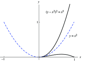
Figure 3. A ramphoid cusp.

In general one obtains the divisor at infinity $I_{j}$ by making the inverted choice in going from level $j-1$ to level $j$. In the resulting chart, $I_{j}$ is given by the vanishing of the new coordinate $\mathbf{n}_{j}$. To obtain the prolongations $I_{j}[\ell]$, one continues by making $\ell$ ordinary choices, and $I_{j}[\ell]$ is given by the additional vanishing of $\mathbf{n}_{j+1}$ through $\mathbf{n}_{j+\ell}$.

To compare all these divisors at infinity and their prolongations, let’s pull everything back to a chosen level $k$. The complete inverse image of $I_{j}$ will be denoted in the same way, but now it’s a divisor up on $S(k)$. With this convention, we now have a nest

$$I_{j}\supset I_{j}[1]\supset I_{j}[2]\supset\cdots\supset I_{j}[k-j].$$

Lemma 12.

Working at a point $p\in S(k)$, where $k\geq 2$, consider the focal bundle $\Delta(k)$. Let $3\leq j\leq k$. The loci $N(V)$ and $N(VT^{\tau})$ used in the proof of Lemma 2 to define the $j$th symbol of its Goursat code word at $p$ are the divisor at infinity $I_{j}$ and the prolongation $I_{j-\tau}[\tau]$.

Proof.

This is immediate from the identification of Goursat and monster coordinates given in Lemma 9. ∎

10. Code words redux

In Section 3 we have associated code words with Goursat distributions. We now associate similar code words with points on the monster spaces over a surface $S$, and to focal curve germs on these spaces. We also discuss how these code words are related to each other.

We define an RVT code word to be a finite word in these three symbols, satisfying the following rules:

1. The first symbol is $R$.

2. The symbol $T$ may only be used immediately following a $V$ or $T$.

For Goursat words, by contrast, the first two symbols are required to be $RR$. Given an $RVT$ code word $W$, we associate with it a Goursat word $G(W)$ by this simple procedure: if there is a $V$ in second position, then replace it and any immediately succeeding $T$’s by $R$’s. For example, if $W$ is $RVTTTVRVT$ then $G(W)$ is $RRRRRVRVT$.

10.1. Code words of points

Given a point $p\in S(k)$, the $k$th monster space over a surface $S$, we associate with it an $RVT$ code word of length $k$ by considering where it lies with respect to the divisors at infinity and their prolongations. Since the divisors at infinity arise beginning at level $2$, the first symbol in the code word is an automatic $R$. Here are the rules for assigning the symbol in position $j$:

1. If $p$ lies on the $j$th divisor at infinity $I_{j}$, then the $j$th symbol is $V$.

2. If $p$ lies on the prolongation $I_{h}[\ell]$, where $\ell>0$ and $h+\ell=j$, then the $j$th symbol is $T$.

3. Otherwise the $j$th symbol is $R$.

Rules 1 and 2 appear to clash, but in fact it’s impossible for $p$ to lie on both $I_{j}$ and $I_{h}[\ell]$. To see this, we consider assigning the symbols one step at a time, beginning after the automatic $R$; we look at the sequence of points going up the tower to our specified point on $S(k)$. At each step, we are considering a fiber of $S(j+1)$ over a point $p\in S(j)$, a projective line. Let $q$ be a point on the fiber of $S(j+1)$ over $p$. One point on the fiber is the intersection with the divisor at infinity $I_{j+1}$; if $q$ is this point, then the new symbol is $V$. If $p$ lies on $I_{j}$ or some $I_{h}[\ell]$, there is a second special point on the fiber, the intersection with the prolongation $I_{j}[1]$ or $I_{h}[\ell+1]$; if $q$ is this point, then the new symbol is $T$. These two special points are distinct. This description also makes it clear that the code word associated with a point satisfies rule 2 for RVT code words.

Example 13.

For the point $p$ of Example 6 the associated RVT code word is $RVTVR$; for the origin of the chart ${\mathcal{C}}(oioio)$ used there, the RVT code word is $RVTVT$.

10.2. Code words of focal curve germs

To obtain the RVT code word of a regularizable focal curve germ $C(k)$ on $S(k)$, lift it upward through the monster tower until you reach the regularization level $r$. The RVT code word records how the successive lifts meet the divisors at infinity $I_{k+2}$ through $I_{r}$, with a $V$ indicating that we are on the divisor at infinity, a $T$ indicating that we are on the prolongation of a divisor at infinity, and $R$ being used otherwise. Also use an $R$ in the first position, i.e., ignore the divisor at infinity $I_{k+1}$ and its prolongations, as well as those of the prior divisors at infinity $I_{2}$ through $I_{k}$. To explain the process in a slightly different two-step way:

1. Record how the curve and its lifts meet the divisors at infinity $I_{k+1}$ through $I_{r}$ and their prolongations.

2. If the resulting word begins with $VT^{\tau}$, replace this string by $R^{\tau+1}$.

The first step of this process produces a word ending with a critical symbol $V$ or $T$, but this symbol may be changed to $R$ in the second step. As a special case, we associate a code word with a curve $C$ on a surface $S$. Here there is no divisor at infinity on $S(1)$, so that the initial $R$ is automatic (unless the germ is nonsingular, in which case the word is empty), and the final symbol will definitely be critical.

Example 14.

For the curve germ $C$ of Example 6 (whose regularization level is 4), the associated RVT code word is $RVTV$; for $C(1)$ through $C(4)$, each of which also has regularization level 4, the associated code words are $RRV$, $RV$, $R$, and the empty word. The fifth lift $C(5)$ has regularization level 5 and its code word is likewise empty.

The reason we make this construction for focal curve germs, rather than just curves on surfaces, is that it gives us the flexibility to calculate other invariants recursively. For example, it is used in the subsequent Section 12 to develop a front-end recursion for Puiseux characteristics.

By definition, all of our code words thus far are finite. For later usage, however, it is convenient to associate a code word of infinite length with a focal curve germ, simply by padding out with an infinite string of $R$’s. None of the invariants considered in this paper is altered when one appends $R$’s to the end of a code word; thus it makes sense to speak of the invariants associated with such infinite words. For example, $PC(RVVRRR\dots)=PC(RVV)=[3;5]$.

One could assign a code word to a nonregularizable focal curve germ, but such a word would be of infinite length and would contain an infinite string of $T$’s; we will not develop a theory of these words.

10.3. Words of points vs. words of Goursat germs

Theorem 15.

Working at a point $p\in S(k)$, consider the focal bundle $\Delta(k)$. The Goursat word associated with $\Delta(k)$ at $p$ is $G(W)$, where $W$ is the RVT code word associated with $p$.

Proof.

We compare the rules for computing the Goursat word of $\Delta(k)$ at $p$ with the rules for computing $G(W)$, where $W$ is the RVT code word associated with $p$. Because of the recursive nature of both sets of rules, it suffices to show that they give the same result in the final position.

Lemma 12 tells us that, for $k\geq 3$,

$$\text{$\Delta(k)$ is singular at $p$}\iff p\in I_{k}.$$

Thus the rules for whether to use a $V$ in the final position of the code word agree. Now suppose $k\geq\tau+3$, where $\tau\geq 1$, and that $\pi(p)\in N(VT^{\tau-1})$, where $\pi:S(k)\to S(k-1)$ is projection. Then, again using Lemma 12,

the Goursat word of $$\;\Delta(k)\;\text{at $p$ has final symbol $T$}$$

$$\iff p\in N(VT^{\tau})$$

$$\iff p\in I_{k-\tau}[\tau]$$

$$\iff\text{the RVT code word of $p$ has final symbol $T$.}$$

In all other situations, both sets of rules dictate a final symbol $R$. ∎

As we have explained in Section 6, the process of finding a point $p_{k}\in S(k)$ representing a given Goursat distribution can be interpreted as finding a sequence of points $p_{1}\in S(1)$, $p_{2}\in S(2)$, etc. Since all points of $S(2)$ represent the same Goursat distribution, we may choose $p_{2}$ wherever we like. In particular we may choose a point $p_{2}$ not lying on the divisor at infinity $I_{2}$; in this case the RVT code word is already a Goursat word.

10.4. Words of points vs. words of focal curves

Suppose that $C(k)$ is a regularizable focal curve germ located at a point $p\in S(k)$. The RVT code word of $p$ and the RVT code word of $C(k)$ record complementary information. Let $C$ be the curve germ on $S$ obtained by projecting $C(k)$. Then the RVT code word of $p$ records the sequence of divisors at infinity and prolongations of such divisors one encounters when lifting $C$ through the tower to recover $C(k)$; it is a word of length $k$. The RVT code word of the germ $C(k)$ records the divisors at infinity and prolongations that one encounters as one continues to lift $C(k)$ until one reaches the regularization level $r$; it is a word of length $r-k$.

Example 16.

Consider this focal curve germ $C(2)$ located at the origin of chart ${\mathcal{C}}(oi)$:

$$x =t^{14}$$

$$y =14(t^{18}+t^{19})$$

$$y^{\prime} =t^{4}(18+19t)$$

$$x^{\prime} =\frac{14t^{10}}{72+95t}$$

The code word of $p=(0,0;0,0)$ is $RV$. The regularization level is 7, and the code word of of $C(2)$ is $RRVRV$. Compare these code words with the code word of $C$:

$$RV|TTVRV$$

We have inserted a vertical slash to indicate how one can recover the words of $p$ and $C(2)$; to obtain a valid RVT code word, one needs to replace the initial two $T$’s by $R$’s.

For a curve germ $C$ on $S$, its code word is the same as the word of the location of $C(r)$ on $S(r)$. More generally, as the example illustrates, one can find the code word of $C(k)$ on $S(k)$ by finding the code word of the location of $C(r)$, lopping off the first $k$ symbols, and then replacing $V$’s and $T$’s as necessary to obtain a valid RVT code word.

Example 17.

In Example 16, the location of $C(7)$ in chart ${\mathcal{C}}(oiooioi)$ is

$$(0,0;0,0,0,0,0,\tfrac{8707129344}{1225},0)$$

and the code word of this point is $RVTTVRV$.

Going in the other direction, given a point $p\in S(k)$ we can find a regular curve germ $C$ in $S$ whose $k$th lift passes through $p$; one simply specifies appropriate parameterizations of the two active coordinates and obtains the other parametric equations by integration. The code word of $C$ is then the same as the code word of $p$.

10.5. The lifted word

Suppose that $W$ is the RVT code word associated with a regularizable focal curve germ $C(k)$ on $S(k)$. The code word of its lift $C(k+1)$ is the lifted word $L(W)$ obtained from $W$ by this recipe:

• Remove the first symbol $R$.

• If the new first symbol is $V$, replace it by $R$, and likewise replace any immediately succeeding $T$’s by $R$’s. Stop when you reach the next $R$, the next $V$, or the end of the word.

Observe that this lifting procedure also applies to an infinite word.

Example 18.

If $W$ is $RVTTVRVRV$, then $L(W)$ is $RRRVRVRV$.

Going in the opposite direction, assume that we know $L(W)$ and want to know the possibilities for $W$. There is a choice in the first step:

1. Any string $R^{\tau}$ at the beginning of $L(W)$ can be replaced by $VT^{{\tau}-1}$. The choice ${\tau}=0$ is allowed; this means don’t make a replacement at all.

2. Put the symbol $R$ at the beginning.

Example 19.

If $L(W)$ is $RRRVRVRV$, then there are four possibilities for $W$:

$$\begin{gathered}\text{\emph{RRRRVRVRV}}\\ RVRRVRVRV\\ RVTRVRVRV\\ RVTTVRVRV\\ \end{gathered}$$

11. Comparison with embedded resolution

As noted in the Introduction, singularity theorists working in the context of algebraic geometry tend to work with point blowups of varieties rather than Nash modifications. The ideas and calculations of earlier sections have counterparts in this context, which we now briefly explain. For a related treatment, see [16], especially Sections 9 and 14.

If we begin, as in Section 8, with coordinates $x=x_{0}$ and $y=y_{0}$ on a neighborhood $U$ on the surface $S$ which contains point $p$, then we may define blowup coordinates on the $k$th blowup $S\{k\}$ of $S$ in a recursive manner: the new coordinate is either

$$y_{j+1}=(y_{j}-y_{j}(p_{k-1}))/(x_{i}-x_{i}(p_{k-1}))$$

or

$$x_{i+1}=(x_{i}-x_{i}(p_{k-1}))/(y_{j}-y_{j}(p_{k-1})).$$

where $p_{k-1}$ denotes a point of $S\{k-1\}$ in the fiber over $p$. The sequence of points and the choice of which of the two formulas to use is dictated by the curve on $S$ which one is studying. Note the contrast with the monster construction, which is carried out in a uniform manner, no matter what curve is eventually to be studied.

Example 20.

Working with the curve $C$ parameterized by $x=t^{5}$, $y=t^{7}$, the blowup coordinate calculation over the origin analogous to that of Example 6 is

$$y_{1} =y/x=t^{2}$$

$$x_{1} =x/y_{1}=t^{3}$$

$$x_{2} =x_{1}/y_{1}=t$$

$$y_{2} =y_{1}/x_{2}=t$$

$$y_{3} =y_{2}/x_{2}=1\,.$$

From this we see that the strict transform $C_{3}\subset S\{3\}$ is nonsingular.

In the context of embedded resolution, the symbols of the RVT code of Subsection 10.2 have the following meanings:

• The first symbol is automatically $R$.

• The symbol in position $j$ is $V$ if the strict transform $C_{j}$ meets the strict transform of the exceptional divisor $E_{j-1}$.

• The symbol in position $j$ is $T$ if $C_{j}$ meets the strict transform of some earlier exceptional divisor $E_{i}$ (with $i<j-1$). This will necessarily be the same exceptional divisor that it met at the prior level.

• The symbol in position $j$ is $R$ if $C_{j}$ meets only the newest exceptional divisor $E_{j}$.

We say that the strict transform $C_{j}$ is regular if it is nonsingular and if it transverse to all the exceptional divisors that it meets. The regularity level is the lowest level at which these conditions are met; this definition agrees with that of Section 7.

12. Puiseux characteristics

12.1. The Puiseux characteristic of a focal curve germ

The Puiseux characteristic is a well-known invariant of a curve germ on a surface $S$, but we wish to extend it to a broader context and relate it to the RVT code. Let $p$ be a point on $S(k)$ and let $C(k)$ be a regularizable focal curve germ located at $p$. Choose an ordered pair $(X,Y)$ of coordinate functions vanishing at $p$, such that

• the differentials $dX$ and $dY$ are independent linear functionals on the focal plane at $p$, and

• $X$ has the smallest possible order of vanishing.

Denoting this order by $n$, introduce a parameter $t$ for which $X=t^{n}$. Then $Y$ may be expressed as a formal power series

$$Y=\sum a_{i}t^{i}$$ (12.1)

where we write just those terms for which $a_{i}\neq 0$. (To say this another way, we write $Y$ as a fractional power series $Y=\sum a_{i}X^{i/n}$.) An exponent in this series is called essential or characteristic if it is not divisible by the greatest common divisor of the smaller exponents. In this definition we count $n$ as an essential exponent; thus the first essential exponent appearing in (12.1) is the first exponent (if any) not divisible by $n$. The set of essential exponents $\{n,\lambda_{1},\dots,\lambda_{g}\}$ is finite and their greatest common divisor is 1. Letting $\lambda_{0}=n$, we define the Puiseux characteristic to be

$$[\lambda_{0};\lambda_{1},\dots,\lambda_{g}].$$

For example, for the focal curve $C$ parameterized by

$$x =s^{4}$$

$$y =s^{6}+s^{7}$$

$$y^{\prime} =\tfrac{3}{2}s^{2}+\tfrac{7}{4}s^{3}$$

we may take our first coordinate function to be $y^{\prime}$ and thus use parameter $t=s\sqrt{\frac{3}{2}+\frac{7}{4}s}$. For second coordinate we may use $x$, whose expansion in the new parameter is

$$x=\tfrac{4}{9}t^{4}-\tfrac{28\sqrt{6}}{81}\,t^{5}+\cdots$$

the first term being inessential. The Puiseux characteristic is $[2;5]$. Observe that $y$ may not be used as our second coordinate function, since $dy=y^{\prime}dx=0$ on the focal plane at $p$.

12.2. The front-end recursion for Puiseux characteristic

In what follows, we show that the RVT code word associated with a regularizable focal curve determines its Puiseux characteristic. As we will see, the Puiseux characteristic can be computed by either of two recursions:

1. A front-end recursion whose step size is a single symbol of the word.

2. A back-end recursion whose step size is a block of symbols.

Here we state the front-end recursion and prove that it is valid, i.e., that it correctly computes the Puiseux characteristic of each focal curve. Subsequently we will describe the back-end recursion and prove that it is a consequence of the front-end recursion; thus it is likewise valid.

The front-end recursion uses the notion of the lifted word $L(W)$ of an RVT code word $W$, as defined in Section 10.

Theorem 21.

Suppose that $C(k)$ is a regularizable focal curve germ located at a point $p$ on $S(k)$. Its associated code word $W$ determines its Puiseux characteristic. If $W$ has no critical symbols, then the associated Puiseux characteristic, denoted $\operatorname{PC}(W)$, is $[1;]$. In general the Puiseux characteristic is determined recursively by the following rules. Suppose that

$$\operatorname{PC}(W)=[\lambda_{0};\lambda_{1},\dots,\lambda_{g}].$$

1. The word $W$ begins with $RR$ if and only if $\lambda_{1}>2\lambda_{0}$. In this case, $\operatorname{PC}(L(W))$ is obtained from $\operatorname{PC}(W)$ by keeping $\lambda_{0}$ and subtracting it from all other entries:

   $$\operatorname{PC}(L(W))=[\lambda_{0};\lambda_{1}-\lambda_{0},\dots,\lambda_{g}-\lambda_{0}].$$

2. The word $W$ begins with $RVT^{\tau}R$ or is $W=RVT^{\tau}$ if and only if

   $$\lambda_{0}=({\tau}+2)(\lambda_{1}-\lambda_{0})\quad\text{and}\quad\lambda_{1}=({\tau}+3)(\lambda_{1}-\lambda_{0}).$$

   In this case

   $$\operatorname{PC}(L(W))=[\lambda_{1}-\lambda_{0};\lambda_{2}-(\lambda_{1}-\lambda_{0}),\dots,\lambda_{g}-(\lambda_{1}-\lambda_{0})].$$

   (Note that this Puiseux characteristic is shorter.)

3. The word $W$ begins with $RVT^{\tau}V$ if and only if

   $$({\tau}+1)(\lambda_{1}-\lambda_{0})<\lambda_{0}<({\tau}+2)(\lambda_{1}-\lambda_{0}).$$

   In this case

   $$\operatorname{PC}(L(W))=[\lambda_{1}-\lambda_{0};\lambda_{0},\lambda_{2}-(\lambda_{1}-\lambda_{0}),\dots,\lambda_{g}-(\lambda_{1}-\lambda_{0})].$$

Example 22.

The Puiseux characteristics associated with the four words of Example 19 are

$$\operatorname{PC}(RRRRVRVRV) =[8;36,38,39]$$

$$\operatorname{PC}(RVRRVRVRV) =[16;24,36,38,39]$$

$$\operatorname{PC}(RVTRVRVRV) =[24;32,36,38,39]$$

$$\operatorname{PC}(RVTTVRVRV) =[28;36,38,39]$$

The first word is covered by Theorem 21(A), the next two by (B), and the last word by (C). In each case $L(W)$ is $RRRVRVRV$, so that $\operatorname{PC}(L(W))=[8;28,30,31]$.

The formulas of Theorem 21 already appear in Theorem 3.5.5 of Wall’s textbook [22], but we remark that the circumstances are different in several ways: Wall’s formulas apply to a curve on a surface, a special case of a focal curve; they are obtained using blowups rather than lifts (i.e., Nash modifications); and he doesn’t invoke RVT code words. Nevertheless our proof is similar.

Proof.

Let $X$ and $Y$ be chosen in accordance with our definition of Puiseux characteristic:

$$X =t^{\lambda_{0}}$$

$$Y =\sum a_{i}t^{i}.$$

We may choose $Y$ so that the first term in its series is $a_{\lambda_{1}}t^{\lambda_{1}}$. For the lifted curve we have available a new coordinate function .

$$Y^{\prime}=dy/dx=\sum\frac{i}{\lambda_{0}}a_{i}t^{i-\lambda_{0}}.$$

If $\lambda_{1}>2\lambda_{0}$, then $X$ continues to have the lowest order of vanishing; thus $(X,Y^{\prime})$ is an appropriate pair of coordinate functions for computing the Puiseux characteristic of the lifted curve, and we obtain the formula of (A). The next stage in lifting involves $Y^{\prime\prime}=dY/dX$, so that the code word begins with $RR$.

If $\lambda_{1}<2\lambda_{0}$, then $\lambda_{1}-\lambda_{0}<\lambda_{0}$ and we can use $(Y^{\prime},X)$ as an appropriate ordered pair of coordinate functions. Let $[\widetilde{\lambda}_{0};\widetilde{\lambda}_{1},\ldots]$ be the Puiseux characteristic of the lifted curve; we observe that $\widetilde{\lambda}_{0}=\lambda_{1}-\lambda_{0}$. To compute the other characteristic exponents we need to invert the fractional power series for $Y^{\prime}$. The formulas for this inversion are well-known: we apply [4, Proposition 5.6.1], replacing Casas-Alvero’s $[n;m_{1},\dots]$ by $[\lambda_{1}-\lambda_{0};\widetilde{\lambda}_{1},\dots]$ and his $[\overline{n};\overline{m}_{1},\dots]$ by $[\lambda_{0};\lambda_{1}-\lambda_{0},\dots]$. The proposition tells us that there are two mutually exclusive possibilities:

• The leading characteristic exponent $\lambda_{1}-\lambda_{0}$ divides $\lambda_{0}$, and the other characteristic exponents are determined by

  $$(\lambda_{i+1}-\lambda_{0})+\lambda_{0}=\widetilde{\lambda}_{i}+(\lambda_{1}-\lambda_{0}).$$

• The first two characteristic exponents are $\lambda_{1}-\lambda_{0}$ and $\widetilde{\lambda}_{1}=\lambda_{0}$; the remaining characteristic exponents are determined by

  $$(\lambda_{i}-\lambda_{0})+\lambda_{0}=\widetilde{\lambda}_{i}+(\lambda_{1}-\lambda_{0}).$$

These two possibilities lead to the formulas for $\operatorname{PC}(L(W))$ of (B) and (C).

In order to compute the associated code word, we examine the successive derivatives $X^{\prime},X^{\prime\prime},X^{(3)},\dots$ of $X$ with respect to $Y^{\prime}$. The order of vanishing in $t$ of $X^{(i)}$ is $(i+1)\lambda_{0}-i\lambda_{1}$. In case (B), let ${\tau}$ be the nonnegative integer for which $\lambda_{0}=({\tau}+2)(\lambda_{1}-\lambda_{0})$. In this case the order of vanishing of $X^{(i)}$ is $({\tau}+2-i)(\lambda_{1}-\lambda_{0})$, which is positive when $i<{\tau}+2$ and becomes zero when $i={\tau}+2$. Thus when we evaluate at $t=0$ we obtain 0 for the first ${\tau}+1$ derivatives, whereas $X^{({\tau}+2)}$ has a nonzero value. Thus the code word begins with $RVT^{{\tau}}$; if this is not the entire word then the next symbol is $R$. Similarly, in case (C) we let ${\tau}$ be such that

$$({\tau}+1)(\lambda_{1}-\lambda_{0})<\lambda_{0}<({\tau}+2)(\lambda_{1}-\lambda_{0}),$$

and observe that the first ${\tau}+1$ derivatives evaluate to 0. The next derivative $X^{({\tau}+2)}$ becomes infinite at $t=0$, which means that the associated symbol is $V$. Thus the code word begins with $RVT^{\tau}V$. ∎

Here we restate the recipes of Theorem 21 in a manner better suited for straightforward calculation.

Theorem 23.

Suppose that the Puiseux characteristic of $L(W)$ is

$$\operatorname{PC}(L(W))=[\lambda_{0};\lambda_{1},\dots,\lambda_{g}].$$

1. If $W$ begins with $RR$, then $\operatorname{PC}(W)=[\lambda_{0};\lambda_{1}+\lambda_{0},\dots,\lambda_{g}+\lambda_{0}]$.

2. If $W$ begins with $RVT^{\tau}R$ or if $W=RVT^{\tau}$, then

   $$\operatorname{PC}(W)=[({\tau}+2)\lambda_{0};({\tau}+3)\lambda_{0},\lambda_{1}+\lambda_{0},\dots,\lambda_{g}+\lambda_{0}].$$

   (This is a longer Puiseux characteristic.)

3. If $W$ begins with $RVT^{\tau}V$, then $\operatorname{PC}(W)=[\lambda_{1};\lambda_{1}+\lambda_{0},\dots,\lambda_{g}+\lambda_{0}]$.

Example 24.

Let $W=RRVTRRRVTTTV$. To compute the Puiseux characteristic using the front-end recursion, we start with

$$\operatorname{PC}(R)=[1;\ ].$$

Theorem 23(B) with $\tau=0$ gives

$$\operatorname{PC}(RV)=[2;3].$$

Then using Theorem 23(A) three times gives

$$\operatorname{PC}(RRRRV)=[2;9].$$

Theorem 23(C) gives

$$\operatorname{PC}(RVTTTV)=[9;11].$$

Using Theorem 23(A) four times gives

$$\operatorname{PC}(RRRRRVTTTV)=[9;47].$$

Then Theorem 23(B) with $\tau=1$ gives

$$\operatorname{PC}(RVTRRRVTTTV)=[27;36,56].$$

Finally, Theorem 23(A) gives

$$\operatorname{PC}(RRVTRRRVTTTV)=[27;63,83].$$

12.3. The back-end recursion for Puiseux characteristic

We now turn to the back-end recursion. This is similar to what is found in [18, Section 3.8] and [20], but our circumstances are slightly broader and the details of our recursion are slightly different. A contiguous substring in an RVT code word is called critical if the last symbol is $V$ or $T$; we call it entirely critical if each of its symbols is $V$ or $T$ (i.e., if it contains no $R$’s). Appending an $R$ to the end of a code word doesn’t change the associated Puiseux characteristic, and for a word consisting entirely of $R$’s (including the empty word) the associated Puiseux characteristic is $[1;]$. Thus the back-end recursion deals with critical words.

We first define two auxiliary functions $E_{T}$ and $E_{V}$ acting on ordered pairs of positive integers:

$$E_{T}[a;b] =[a;a+b]$$

$$E_{V}[a;b] =[b;a+b].$$

We recursively define a function $E$ from entirely critical strings to ordered pairs of positive integers:

$$E(\text{empty string}) =[1;2]$$

$$E(TQ) =E_{T}(E(Q))$$

$$E(VQ) =E_{V}(E(Q)).$$

(In these formulas $Q$ denotes an entirely critical string, possibly empty.) In fact, we can extend it to strings of the form $R^{{\rho}}Q$, where $Q$ is entirely critical, by defining $E_{R}[a;b]=[a;a+b]$ (so that $E_{R}$ is the same as $E_{T}$) and

$$E(RQ)=E_{R}(E(Q)).$$

For example,

$$E(R^{4}V^{2})=E_{R}\circ E_{R}\circ E_{R}\circ E_{R}\circ E_{V}\circ E_{V}[1;2]=[3;17].$$

Theorem 25.

The Puiseux characteristic of a critical RVT code word is determined as follows. Write the code word $W$ as $PR^{{\rho}}Q$, where $P$ is either empty or critical, ${\rho}\geq 1$, and $Q$ is entirely critical. (Note that the substring $Q$ must begin with a $V$, since we want $W$ to be a valid code word.) Suppose that

$$\operatorname{PC}(P) =[\lambda_{0};\lambda_{1},\ldots,\lambda_{g}]\quad\text{and}$$

$$E(R^{{\rho}}Q) =[a;b].$$

Then

$$\operatorname{PC}(W)=[a\lambda_{0};a\lambda_{1},\ldots,a\lambda_{g},a\lambda_{g}+b-2a].$$

If $W=R^{{\rho}}Q$, i.e., if $P$ is the empty word, then (applying our rules with $g=0$) we have

$$\operatorname{PC}(P)=[1;]\quad\text{and}\quad\operatorname{PC}(W)=[a;b-a].$$

In other words, the back-end recursion tells us that

$$\operatorname{PC}(R^{\rho}Q)=E(R^{{\rho}-1}Q).$$ (12.2)

Within this recursion, the subroutine of computing the function $E$ is a front-end recursion. In fact it’s essentially a special case of the front-end recursion of Theorem 23. Indeed, we can prove formula (12.2) by induction on the length of the word. To begin, we remark that for a word with a single $V$ we have agreement:

$$\operatorname{PC}(R^{\rho}VT^{\tau}) =[\tau+2;\rho(\tau+2)+1]$$

$$E(R^{\rho-1}VT^{\tau}) =[\tau+2;\rho(\tau+2)+1].$$

Thus in the inductive step it suffices to consider a word $W=R^{\rho}VT^{\tau}Q^{\prime}$, where $Q^{\prime}$ begins with a $V$. Let $\operatorname{PC}(L(W))=[\lambda_{0};\lambda_{1}]$. There are two cases to consider:

• If $\rho\geq 2$, then by the inductive hypothesis

  $$\operatorname{PC}(R^{\rho-1}VT^{\tau}Q^{\prime})=E(R^{\rho-2}VT^{\tau}Q^{\prime})=[\lambda_{0};\lambda_{1}].$$

  According to Theorem 23(A),

  $$\operatorname{PC}(R^{\rho}VT^{\tau}Q^{\prime})=[\lambda_{0};\lambda_{1}+\lambda_{0}],$$

  in agreement with

  $$E(R^{\rho-1}VT^{\tau}Q^{\prime})=E_{R}(E(R^{\rho-2}VT^{\tau}Q^{\prime}))=[\lambda_{0};\lambda_{1}+\lambda_{0}].$$

• If $\rho=1$, then by the inductive hypothesis

  $$\operatorname{PC}(R^{\tau+1}Q^{\prime})=E(R^{\tau}Q^{\prime})=[\lambda_{0};\lambda_{1}].$$

  According to Theorem 23(C),

  $$\operatorname{PC}(RVT^{\tau}Q^{\prime})=[\lambda_{1};\lambda_{1}+\lambda_{0}],$$

  in agreement with

  $$E(VT^{\tau}Q^{\prime})=E_{V}(T^{\tau}Q^{\prime}))=E_{V}(R^{\tau}Q^{\prime})=[\lambda_{1};\lambda_{1}+\lambda_{0}].$$

Example 26.

As in Example 24, let $W=RRVTRRRVTTTV$. To compute its Puiseux characteristic using the back-end recursion, we start by using formula (12.2):

$$\operatorname{PC}(RRVT)=E(RVT)=[3;7].$$

Now compute $E(RRRVTTTV)=[9;38]$, so that Theorem 25 gives

$$\operatorname{PC}(RRVTRRRVTTTV)=[9\cdot 3;9\cdot 7,9\cdot 7+38-2\cdot 9]=[27;63,83].$$

Proof of Theorem 25.

To prove the formula for $\operatorname{PC}(W)$, we use induction on the length of $W$. For a word with a single entirely critical block, we have already confirmed formula (12.2). Thus in the inductive step it suffices to consider a word $W=PR^{{\rho}}Q$, where $P$ is critical, ${\rho}\geq 1$, and $Q$ is entirely critical. We remark that the lifted word is

$$L(W)=L(P)R^{{\rho}}Q.$$

Let $\operatorname{PC}(L(P))=[\lambda_{0};\lambda_{1},\ldots,\lambda_{g}]$ and $E(R^{{\rho}}Q)=[a;b]$. By the inductive hypothesis we know that

$$\operatorname{PC}(L(W))=[a\lambda_{0};a\lambda_{1},\ldots,a\lambda_{g},a\lambda_{g}+b-2a].$$

We now consider the three cases of Theorem 23:

1. If $P$ begins with $RR$, then 23(A) tells us that

   $$\operatorname{PC}(P) =[\lambda_{0};\lambda_{1}+\lambda_{0},\dots,\lambda_{g}+\lambda_{0}]$$

   $$\operatorname{PC}(W) =[a\lambda_{0};a\lambda_{1}+a\lambda_{0},\dots,a\lambda_{g}+a\lambda_{0},a\lambda_{g}+b-2a+a\lambda_{0}]$$

   $$=[a\lambda_{0};a(\lambda_{1}+\lambda_{0}),\dots,a(\lambda_{g}+\lambda_{0}),a(\lambda_{g}+\lambda_{0})+b-2a].$$

2. If $P$ begins with $RVT^{\tau}R$ or if $P=RVT^{\tau}$, then 23(B) tells us that

   $$\operatorname{PC}(P) =[({\tau}+2)\lambda_{0};({\tau}+3)\lambda_{0},\lambda_{1}+\lambda_{0},\dots,\lambda_{g}+\lambda_{0}]$$

   $$\operatorname{PC}(W) =[({\tau}+2)a\lambda_{0};({\tau}+3)a\lambda_{0},$$

   $$\qquad a\lambda_{1}+a\lambda_{0},\dots,a\lambda_{g}+a\lambda_{0},a\lambda_{g}+b-2a+a\lambda_{0}]$$

   $$=[a({\tau}+2)\lambda_{0};a({\tau}+3)\lambda_{0},$$

   $$\qquad a(\lambda_{1}+\lambda_{0}),\dots,a(\lambda_{g}+\lambda_{0}),a(\lambda_{g}+\lambda_{0})+b-2a].$$

3. If $P$ begins with $RVT^{\tau}V$, then 23(C) tells us that

   $$\operatorname{PC}(P) =[\lambda_{1};\lambda_{1}+\lambda_{0},\dots,\lambda_{g}+\lambda_{0}]$$

   $$\operatorname{PC}(W) =[a\lambda_{1};a\lambda_{1}+a\lambda_{0},\dots,a\lambda_{g}+a\lambda_{0},a\lambda_{g}+b-2a+a\lambda_{0}]$$

   $$=[a\lambda_{1};a(\lambda_{1}+\lambda_{0}),\dots,a(\lambda_{g}+\lambda_{0}),a(\lambda_{g}+\lambda_{0})+b-2a].$$

∎

12.4. From Puiseux characteristic to code word

The Puiseux characteristic and the RVT code word are equivalent pieces of information. Having obtained two recursive recipes for computing the Puiseux characteristic from a given code word, we now explain how to reverse these recipes.

In the case of front-end recursion, the reversed recipe can be inferred from the cases of Theorem 21. We illustrate the process by an example.

Example 27.

Suppose that $\operatorname{PC}(W)=[10;15,27]$. This puts us in case (B) of Theorem 21 with ${\tau}=0$; thus $W$ begins with $RVR$ and $\operatorname{PC}(L(W))=[5;22]$. Invoking case (A) three times, we learn that $L(W)$, $L^{2}(W)$, and $L^{3}(W)$ all begin with $RR$, so that

$$W=RVRRR\dots$$

and $\operatorname{PC}(L^{4}(W))=[5;7]$. Using case (C) with ${\tau}=1$, we find that $L^{4}(W)$ begins with $RVTV$ and that $\operatorname{PC}(L^{5}(W))=[2;5]$. By case (A), $L^{5}(W)$ begins with $RR$ (but this is redundant information) and $\operatorname{PC}(L^{6}(W))=[2;3]$. Finally we use case (B) with ${\tau}=0$ to infer that $L^{6}(W)$ begins with $RVR$. Thus

$$W=RVRRRVTVR.$$

For the back-end recursion, the reverse recipe is essentially what is explained in [18, Section 3.8.4] and in [20, Section 2.4], although there the circumstances are slightly different. We denote the map from Puiseux characteristics to critical RVT code words by $\operatorname{CW}$. We first describe an auxiliary map which we denote by $\operatorname{Euc}$; given a pair $(a,b)$ of relatively prime positive integers with $a<b$, it produces a string of $V$’s and $T$’s. We define $\operatorname{Euc}(1,2)$ to be the empty word. Otherwise we recursively define

$$\operatorname{Euc}(a,b)=\begin{cases}V\text{ followed by }\operatorname{Euc}(b-a,a)\quad\text{ if }b<2a,\\ T\text{ followed by }\operatorname{Euc}(a,b-a)\quad\text{ if }b>2a.\end{cases}$$

For example,

$$\operatorname{Euc}(2,7)=T\operatorname{Euc}(2,5)=TT\operatorname{Euc}(2,3)=TTV.$$

And here is an example using Fibonacci numbers: $\operatorname{Euc}(F_{k+2},F_{k+3})=V^{k}$.

We now describe the $\operatorname{CW}$ map. First suppose that the Puiseux characteristic is simply $[\lambda_{0};\lambda_{1}]$. To obtain $\operatorname{CW}[\lambda_{0};\lambda_{1}]$, first compute $\operatorname{Euc}(\lambda_{0},\lambda_{1})$, then replace the initial string of $T$’s (if any) by the same-length string of $R$’s and put a single $R$ in front. For example, $\operatorname{CW}[2;7]=RRRV$. For a longer Puiseux characteristic $[\lambda_{0};\lambda_{1},\dots,\lambda_{k+1}]$, let

$$a =\operatorname{GCD}(\lambda_{0},\lambda_{1},\dots,\lambda_{k}),$$

$$s =\left\lfloor\frac{\lambda_{k+1}-\lambda_{k}}{a}\right\rfloor+1,$$

$$b =a\left(\operatorname{frac}\left(\frac{\lambda_{k+1}-\lambda_{k}}{a}\right)+1\right)$$

(using the floor function and the fractional-part function as indicated). Then inductively define

$$\operatorname{CW}[\lambda_{0};\lambda_{1},\dots,\lambda_{k+1}]=\operatorname{CW}\left[\frac{\lambda_{0}}{a};\frac{\lambda_{1}}{a},\dots,\frac{\lambda_{k}}{a}\right]R^{s}\operatorname{Euc}(a,b).$$

For example,

$$\operatorname{CW}[4;6,7]=\operatorname{CW}[2;3]R\operatorname{Euc}(2,3)=RVRV$$

(since $a=2$, $s=1$, and $b=3$).

12.5. The Puiseux characteristics of points and Goursat germs

Given a point $p_{k}\in S(k)$, we associate with it a well-defined Puiseux characteristic, namely the Puiseux characteristic associated with any regular focal curve germ passing through $p_{k}$. Similarly, given a Goursat germ of corank $k$, recall from Section 10.3 that we can choose a representative point on $S(k)$ that avoids the second divisor at infinity $I_{2}$. All such points have the same associated Puiseux characteristic. Thus we may speak of the Puiseux characteristic of a Goursat germ. This is a restricted Puiseux characteristic, meaning that it satisfies the inequality $\lambda_{1}>2\lambda_{0}$. If instead we had chosen a point lying on $I_{2}$, to obtain the restricted Puiseux characteristic we would need to replace $\lambda_{0}$ by the remainder obtained by dividing $\lambda_{1}$ by $\lambda_{0}$.

The version in [18] and [20] of the algorithm for obtaining the Puiseux characteristic is applied to code words in which the first symbol is at level 3. In comparison with our algorithm, here’s how it works: first put $RR$ at the beginning, thus obtaining a Goursat word, and then apply our algorithm. Note that this yields a restricted Puiseux characteristic. For the algorithm in the opposite direction, begin with a restricted Puiseux characteristic. If we apply our $\operatorname{CW}$ map, we obtain a code word beginning with $RR$; the algorithm in [18] and [20] jettisons these initial symbols.

13. The multiplicity sequence

One of the standard invariants in the theory of curves on surfaces is the multiplicity sequence, as explained, e.g., in Section 3.5 of [22]. The usual definition employs embedded resolution of singularities, whereas for present purposes we want to use lifting into the monster tower; the two definitions give identical sequences. We also want to generalize the situation, by defining the multiplicity sequence associated with any regularizable focal curve germ.

Consider a regularizable focal curve germ $C(k)$ located at point $p_{k}$ on the monster space $S(k)$. For $j\geq k$, the symbol $m_{j}$ denotes the multiplicity of $C(j)$ at its location $p_{j}$ on $S(j)$. The multiplicity sequence of $C(k)$ is the sequence $m_{k},m_{k+1},m_{k+2},\dots$. Note that $m_{j}$ is the leading entry of the Puiseux characteristic $\operatorname{PC}(L^{j-k}(W))$, where $W$ is the associated infinite code word of Section 10.2. One can regard each multiplicity as being associated with a symbol of the word, except for the leading multiplicity $m_{k}$, as indicated in Figure 4. (The edges will be explained momentarily.) This infinite code word ends in an infinite string of $R$’s, for which each of the associated multiplicities is 1.

Our recursion for computing the Puiseux characteristics of lifted curves yields a recursion for computing the multiplicity sequence from the code word.

Example 28.

For the word $W=RVTVVRRR\dots$, the Puiseux characteristics are as follows:

$$\operatorname{PC}(RVTVV) =[8;11]$$

$$\operatorname{PC}(RRVV) =[3;8]$$

$$\operatorname{PC}(RVV) =[3;5]$$

$$\operatorname{PC}(RV) =[2;3]$$

$$\operatorname{PC}(R) =[1;]$$

$$\operatorname{PC}() =[1;]$$

Thus the multiplicity sequence is $8,3,3,2,1,1,1,\dots$.

An alternative recursion uses the proximity diagram. Since our situation is different from that of Wall [22], we cannot simply cite his definitions, but eventually we will obtain a formula identical to that of his Proposition 3.5.1(iii). Here are our definitions. Looking at the sequence of points $p_{k}$, $p_{k+1}$, $p_{k+2}$, etc., we say that $p_{j}$ is proximate to $p_{i}$ if either $j=i+1$, or $p_{j}$ lies on the prolongation of the divisor at infinity $I_{i+2}$, where $i\geq k$. The proximity diagram represents each point of the sequence by a vertex, with edges recording proximity; we furthermore record the code word, as in Figure 4 (taken from page 52 of [22] and modified). The diagram continues to the right indefinitely, but the essential information is visible in that portion to the left of the last critical symbol.

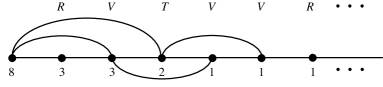
Figure 4. A proximity diagram.

We observe that the code word determines the diagram. The edges between successive vertices are automatic. The other edges are determined in the following way: for each substring $VT^{\tau}$, let $i$ be the position of the vertex corresponding to the $V$, and draw edges from each vertex of the substring to the vertex in position $i-2$. The multiplicities to the right of the last critical symbol are 1’s.

Theorem 29.

The multiplicity $m_{i}$ is given by $\sum m_{j}$, summing over all $j$ for which $p_{j}$ is proximate to $p_{i}$.

Proof.

We prove this by induction on the length of the code word $W$. In the inductive step we use the three cases of Theorems 21 and 23. Let the Puiseux characteristic of $L(W)$ be $[\lambda_{0};\lambda_{1},\dots,\lambda_{g}]$. In case (A) the word begins with $RR$; thus in the proximity diagram the leftmost vertex is connected only to its neighbor to the right. Theorem 23(A) tells us that the multiplicities of these two vertices are both $\lambda_{0}$. In case (B), the leftmost portion of the proximity diagram is as shown in Figure 5.

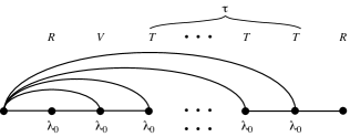
Figure 5. Left portion of the proximity diagram in case (B). There may be additional edges going rightward from the rightmost vertex labeled $T$, but they are irrelevant to the argument.

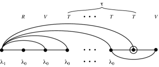
Figure 6. Left portion of the proximity diagram in case (C). There may be additional edges going rightward from the two rightmost vertices labeled $T$, but again they are irrelevant.

There the inductive hypothesis has been used to infer that all the indicated multiplicities are the same. Theorem 23(B) tells us that the multiplicity at the left vertex is $(\tau+2)\lambda_{0}$, in accord with the formula of Theorem 29. In case (C), Theorem 23(C) tells us that the leftmost multiplicity is $\lambda_{1}$. Thus the inductive hypothesis tells us that the leftmost portion of the proximity diagram is as shown in Figure 6. By Theorem 21(A) we infer that

$$PC(L^{i}(W))=PC(R^{\tau}V\cdots)=[\lambda_{0},\lambda_{1}-(i-1)\lambda_{0},\dots]$$

for $1\leq i\leq\tau+1$; then by Theorem 21(B) or (C) we find that the first entry of $PC(L^{\tau+2}(W))$ is $(\lambda_{1}-\tau\lambda_{0})-\lambda_{0}=\lambda_{1}-(\tau+1)\lambda_{0}$. Thus this is the multiplicity associated with the circled vertex. Again this is in accord with the formula of Theorem 29. ∎

14. Vertical orders

For a regularizable focal curve germ $C(k)$ located at $p_{k}\in S_{k}$, let $C(r)$ be its lift to the regularization level $r$. For $k+2\leq j\leq r$, we define the vertical order $\operatorname{VO}_{j}$ to be the intersection number at $p_{r}$ of $C(r)$ and the divisor at infinity $I_{j}$:

$$\operatorname{VO}_{j}:=(C(r)\cdot I_{j})_{p_{r}}$$

Recall that the divisor at infinity $I_{j}$ first appears at level $j$ of the tower. To interpret the intersection number in our definition, one can either use its inverse image on $S(r)$ — it is convenient to continue denoting it by $I_{j}$ — or one can project $C(r)$ to a curve germ on $S(j)$ (likely a singular curve) and compute the intersection number there. By the standard projection formula (for example, see [7, p. 25] or [8, Example 8.1.7]), these procedures give the same result. As a practical matter one computes the vertical order by using a parameterization of $C(r)$, and $\operatorname{VO}_{j}$ is the order of vanishing of the function defining the divisor at infinity $I_{j}$.

The vertical orders vector is

$$\operatorname{VO}(C)=(\operatorname{VO}_{k+2},\operatorname{VO}_{k+3},\dots,\operatorname{VO}_{r})$$

and the restricted vertical orders vector is

$$\operatorname{RO}(C)=(\operatorname{VO}_{k+3},\operatorname{VO}_{k+4},\dots,\operatorname{VO}_{k}).$$

We will soon show that these vectors just depend on the word $W$ associated with $C(r)$; thus the notations $\operatorname{VO}(W)$ and $\operatorname{RO}(W)$ may be used. In fact $\operatorname{RO}(W)$ is determined by the Goursat word $G(W)$ and can thus be interpreted as an invariant of Goursat distributions; this is why we introduce this invariant, which will appear again in our subsequent paper.

Example 30.

Consider a plane curve with code word $W=RVVVRVT$, equivalently Puiseux characteristic $[15;24,25]$. One such curve is $x=t^{15},y=t^{24}+t^{25}$; alternatively one can obtain such a curve by starting in the chart ${\mathcal{C}}(oiiioio)$ with the parameterizations of the active variables $x^{(3)}=1+t$ and $y^{(4)}=t$ and then integrating appropriately. One deduces the following orders of vanishing:

$$\operatorname{ord}_{t}(x) =15$$

$$\operatorname{ord}_{t}(y) =24$$

$$\operatorname{ord}_{t}(y^{\prime}) =9$$

$$\operatorname{VO}_{2}=\operatorname{ord}_{t}(x^{\prime}) =6$$

$$\operatorname{VO}_{3}=\operatorname{ord}_{t}(y^{\prime\prime}) =3$$

$$\operatorname{VO}_{4}=\operatorname{ord}_{t}(x^{\prime\prime}) =3$$

$$\operatorname{ord}_{t}(x^{(3)}) =0$$

$$\operatorname{VO}_{6}=\operatorname{ord}_{t}(y^{(3)}) =2$$

$$\operatorname{ord}_{t}(y^{(4)}) =1$$

The fifth and seventh lifts of the curve do not meet the divisors at infinity $I_{5}$ and $I_{7}$, so that the corresponding vertical orders are zero. Thus $\operatorname{VO}(W)=(6,3,3,0,2,0)$.

For a curve with code word $G(W)=RRVVRVT$, equivalently Puiseux characteristic $[9;24,25]$, we find that $\operatorname{VO}(G(W))=(0,3,3,0,2,0)$.

When one works with ordinary blowups rather than Nash modifications, the vertical order has the following interpretation: $\operatorname{VO}_{j}$ is the intersection number of $C_{j}$ and $E_{j-1}$, where $C_{j}$ is the strict transform of the plane curve $C$ and $E_{j-1}$ is the strict transform of the exceptional divisor arising from the $(j-1)$st blowup. Again as a practical matter, one computes orders of vanishing, as illustrated by the following example.

Example 31.

Working as in Example 30 with the curve $x=t^{15},y=t^{24}+t^{25}$, the orders of vanishing presented there are the same as the orders of vanishing of $x$, $y$, $y_{1}=y/x$, $x_{1}=x/y_{1}$, $y_{2}=x_{1}/y_{1}$, $x_{2}=x_{1}/y_{2}$, $x_{3}=x_{2}/y_{2}$, $y_{3}=y_{2}/(x_{3}-1)$, and $y_{4}=y_{3}/(x_{3}-1)$. Here we have used the blowup coordinates explained in Section 11.

Theorem 32.

For $0\leq j\leq r-2$, we have $\operatorname{VO}_{j+2}=m_{j}-m_{j+1}$. Thus the vertical orders depend only on the word associated with a focal curve germ.

Proof.

Once again we refer to the three cases of Theorem 21, letting $W$ be the word associated with $C_{j}$. In case (A), the multiplicity $m_{j}$ is the leading entry of $PC(W)$ and $m_{j+1}$ is the leading entry of $PC(L(W))$; both of them are $\lambda_{0}$. Since $\lambda_{1}>2\lambda_{0}$, $C_{j+2}$ does not meet the divisor at infinity $I_{j+2}$ and thus $VO_{j+2}=0$. In cases (B) and (C), we have $m_{j}=\lambda_{0}$ and $m_{j+1}=\lambda_{1}-\lambda_{0}$. To see the germ $C_{j+1}$, we need to make the inverted choice, and the order of vanishing of the new coordinate (whose vanishing gives the divisor at infinity) is $\lambda_{0}-(\lambda_{1}-\lambda_{0})$. ∎

15. The small growth sequence

Suppose that $D$ is a distribution on a manifold $M$; let ${\mathcal{E}}$ be its sheaf of sections. We consider its small growth sequence:

$${\mathcal{E}}={\mathcal{E}}^{1}\subset{\mathcal{E}}^{2}\subset{\mathcal{E}}^{3}\subset\dots$$

defined by

$${\mathcal{E}}^{j}={\mathcal{E}}^{j-1}+[{\mathcal{E}}^{j-1},{\mathcal{E}}].$$

Note how this differs from the Lie square sequence in (2.1): at each step we form Lie brackets with vector fields from the beginning distribution. For each point $p\in X$ we let $\operatorname{SG}_{i}$ denote the rank of ${\mathcal{E}}^{i}$ at $p$; we call

$$\operatorname{SG}(D,p)=(\operatorname{SG}_{1},\operatorname{SG}_{2},\ldots)$$

the small growth vector. Simple examples show that this vector may differ from point to point of $M$.

In our subsequent paper, we will consider the small growth vector of a Goursat distribution and related invariants of the small growth sequence, as indicated in the bottom box of Figure 1, as well as their connections to the invariants considered in this paper.

References

- [1] R. L. Bryant, S. S. Chern, R. B. Gardner, H. L. Goldschmidt, and P. A. Griffiths. Exterior differential systems, volume 18 of Mathematical Sciences Research Institute Publications. Springer-Verlag, New York, 1991.
- [2] Robert L. Bryant and Lucas Hsu. Rigidity of integral curves of rank distributions. Invent. Math., 114(2):435–461, 1993.
- [3] Ana Cannas da Silva. Lectures on symplectic geometry, volume 1764 of Lecture Notes in Mathematics. Springer-Verlag, Berlin, 2001.
- [4] Eduardo Casas-Alvero. Singularities of plane curves, volume 276 of London Mathematical Society Lecture Note Series. Cambridge University Press, Cambridge, 2000.
- [5] Alex Castro, Susan Jane Colley, Gary Kennedy, and Corey Shanbrom. A coarse stratification of the monster tower. Michigan Math. J., 66(4):855–866, 2017.
- [6] Susan Jane Colley and Gary Kennedy. The enumeration of simultaneous higher-order contacts between plane curves. Compositio Math., 93(2):171–209, 1994.
- [7] William Fulton. Introduction to intersection theory in algebraic geometry, volume 54 of CBMS Regional Conference Series in Mathematics. Conference Board of the Mathematical Sciences, Washington, DC; by the American Mathematical Society, Providence, RI, 1984.
- [8] William Fulton. Intersection theory, volume 2 of Ergebnisse der Mathematik und ihrer Grenzgebiete. 3. Folge. A Series of Modern Surveys in Mathematics [Results in Mathematics and Related Areas. 3rd Series. A Series of Modern Surveys in Mathematics]. Springer-Verlag, Berlin, second edition, 1998.
- [9] Robin Hartshorne. Algebraic geometry. Springer-Verlag, New York-Heidelberg, 1977. Graduate Texts in Mathematics, No. 52.
- [10] Kenneth Hoffman and Ray Kunze. Linear algebra. Prentice-Hall, Inc., Englewood Cliffs, N.J., second edition, 1971.
- [11] Thomas A. Ivey and J. M. Landsberg. Cartan for beginners: differential geometry via moving frames and exterior differential systems, volume 61 of Graduate Studies in Mathematics. American Mathematical Society, Providence, RI, 2003.
- [12] Frédéric Jean. The car with trailers: characterisation of the singular configurations. ESAIM Contrôle Optim. Calc. Var., 1:241–266, 1995/96.
- [13] Jean-Louis Koszul and Yi Ming Zou. Introduction to symplectic geometry. Science Press Beijing, Beijing; Springer, Singapore, 2019. With forewords by Michel Nguiffo Boyom, Frédéric Barbaresco and Charles-Michel Marle.
- [14] Antonio Kumpera and Ceferino Ruiz. Sur l’équivalence locale des systèmes de Pfaff en drapeau. In Monge-Am père equations and related topics (Florence, 1980), pages 201–248. Ist. Naz. Alta Mat. Francesco Severi, Rome, 1982.
- [15] Richard Montgomery. A tour of subriemannian geometries, their geodesics and applications, volume 91 of Mathematical Surveys and Monographs. American Mathematical Society, Providence, RI, 2002.
- [16] Richard Montgomery, Vidya Swaminathan, and Mikhail Zhitomirskii. Resolving singularities with Cartan’s prolongation. J. Fixed Point Theory Appl., 3(2):353–378, 2008.
- [17] Richard Montgomery and Michail Zhitomirskii. Geometric approach to Goursat flags. Ann. Inst. H. Poincaré Anal. Non Linéaire, 18(4):459–493, 2001.
- [18] Richard Montgomery and Michail Zhitomirskii. Points and curves in the Monster tower. Mem. Amer. Math. Soc., 203(956):x+137, 2010.
- [19] Piotr Mormul. Geometric classes of Goursat flags and the arithmetics of their encoding by small growth vectors. Cent. Eur. J. Math., 2(5):859–883, 2004.
- [20] Corey Shanbrom. The Puiseux characteristic of a Goursat germ. J. Dyn. Control Syst., 20(1):33–46, 2014.
- [21] Shlomo Sternberg. Lectures on differential geometry. Chelsea Publishing Co., New York, second edition, 1983. With an appendix by Sternberg and Victor W. Guillemin.
- [22] C. T. C. Wall. Singular points of plane curves, volume 63 of London Mathematical Society Student Texts. Cambridge University Press, Cambridge, 2004.