Probing Spin-Induced Quadrupole Moments in Precessing Compact Binaries

Abstract

Spin-induced quadrupole moments provide an important characterization of compact objects, such as black holes, neutron stars and black hole mimickers inspired by additional fields and/or modified theories of gravity. Black holes in general relativity have a specific spin-induced quadrupole moment, with other objects potentially having differing values. Different values of this quadrupole moment lead to modifications of the spin precession dynamics, and consequently modifications to the inspiral waveform. Based on the spin-dynamics and the associated precessing waveform developed in our previous work, we assess the prospects of measuring spin-induced moments in various black hole, neutron star, and black-hole mimicker binaries. We focus on binaries in which at least one of the objects is in the mass-gap (similar to the $2.6M_{\odot}$ object found in GW190814). We find that for generic precessing binaries, the effect of the spin-induced quadrupole moments on the precession is sensitive to the nature of the mass-gap object, i.e., whether it is a light black hole or a massive neutron star. So that this is a good probe of the nature of these objects. For precessing black-hole mimicker binaries, this waveform also provides significantly tighter constraints on their spin-induced quadrupole moments than the previous results obtained without incorporating the precession effects of spin-induced quadrupole moments. We apply the waveform to sample events in GWTC catalogs to obtain better constraints on the spin-induced quadrupole moments, and discuss the measurement prospects for events in the O$4$ run of the LIGO-Virgo-KAGRA collaboration.

I Introduction

In the past seven years, the LIGO-Virgo-KAGRA collaboration (LVK) has detected more than one hundred binary black hole merger events, and a handful of events involving neutron stars (be they black hole-neutron star or binary neutron star systems) [1, 2, 3, 4]. In the event catalogs, if the gravitational wave (GW) measurement for the mass of an object within the binary is greater than $5M_{\odot}$, the object has been identified as a “black hole” by convention. Similarly, if the mass is less than $2M_{\odot}$ (less than $3M_{\odot}$ in GWTC-3 [4]), it is identified as a “neutron star”.

While this classification system is convenient for bookkeeping purposes, it comes with two inherent issues. First, if the mass distributions of black holes and neutron stars overlap, we potentially misidentify objects if we only use their masses. Second, this system fails to say anything about objects lying between these bounds, in the so-called mass gap. With the unexpected discovery of the $2.6M_{\odot}$ object in GW190814 (which can be either a heavy neutron star [5, 6] or a light black hole [7, 8, 9, 10]), we are forced to confront this second issue if we want to determine the nature of this and similar objects. The nature of these objects can provide insight into their formation mechanism. For example, these objects may also appear in extreme mass ratio inspirals as relevant sources for space-borne gravitational wave detection [11]. Their relative abundance in “wet” (accretion-disk assisted) [12, 13] and “dry” (scattering assisted) [14, 15] formation channels can be used to constrain supernovae explosion mechanisms, which is related to possible delayed fall-back accretion that strongly affects the remnant mass. Being able to classify the nature of mass-gap objects correctly is increasingly important.

In principle, there are different methods to distinguish between a mass gap neutron star and black hole. While a massive neutron star has an electromagnetic (EM) counterpart (such as short gamma-ray emission and/or kilonova emission), a black hole does not. Consequently, we may distinguish between the two on the basis of the signature of an EM counterpart [16, 17]. This is weighted by the fact that EM counterpart detection is not always available (i.e., see the EM followups for GW190814 [18, 19, 20, 21, 22]) either due to faint emission sources or poor sky localization capacities. The ability to probe the nature of mass-gap objects may also be compromised as the EM signature seems to be greatly influenced by the eccentricity, spin and mass ratio of the system. These are often not accurately constrained by the gravitational wave measurement, in part because a large portion of the parameter space is less explored from the modelling perspective.

Hence, we need a method of distinguishing between a massive neutron star and a light black hole via the gravitational waveform alone. There are several potential gravitational-wave observables that can distinguish between these objects: the tidal deformability, the horizon absorption, and the spin-induced quadrupole moment (SIQM).

The most promising observable for lower-mass ($\leq 2M_{\odot}$) objects should be the (dimensionless) tidal Love number, which is constrained to be $\Lambda(1.4M_{\odot})\leq 800$ for the low-spin prior in GW170817 [23, 24]. However, it is known that the tidal Love number drops dramatically with increasing masses - for objects with masses reaching up to 2.6 $M_{\odot}$, the dimensionless tidal Love number is $\mathcal{O}(1)$ with an uncertainty marginally achievable by 3rd generation detectors [25, 26, 27, 28]. The horizon absorption effect (sometimes referred to as tidal heating), on the other hand, generally enters the waveform phase at $2.5$ Post-Newtonian (PN) order for spinning black holes and $4$PN for non-spinning black holes. According to the discussion in [29] (see also Sec.II.3 in this work), the corresponding effect is smaller than those of other observables. As a result, it appears that measuring the spin-induced quadrupole moment is the only viable approach to discern the nature of mass-gap objects. Because of the quadrupole-curvature coupling, the spin-induced moment affects both the non-precessing part (which decides the phase of the waveform) and the precessing part (which decides the time-dependent rotation of the source frame) of the waveform.

In this work we show that the precessing effect, at least for some configurations, provides a more sensitive probe on the spin-induced quadrupole moment than the non-precessing effect discussed in previous works [30, 31, 32]. In our previous work, we have developed the first precession module of a general waveform model with the effect of spin-induced moments properly accounted for [33]. Here, we apply this waveform model to investigate the measurement uncertainties of the SIQM for various kinds of compact binaries, using Markov-Chain Monte-Carlo (MCMC) simulations. The detectability prospects are promising, assuming the sensitivity of the A^# detector.

The SIQM of an extended object can be written generally as $Q=-\kappa\,\chi^{2}m^{3}$ [30], where $Q$ is the quadrupole moment scalar, $m$ is the object’s mass, $\chi$ its dimensionless spin, and $\kappa$ a dimensionless constant that is one for black holes, and typically greater than one for neutron stars or other objects [25, 34, 35, 36]. As the name, spin induced quadrupole moment, suggests, the quadrupole moment is a result of the deformation to the object induced by spin. This means that the most crucial factor affecting the measurement accuracy of $\kappa$ is the magnitude of the spins of the compact objects - if the spins are zero (or small) the waveform is completely (largely) insensitive to the value of $\kappa$.

Fortunately, we have reason to suspect that objects in the mass gap have relatively large spin, making them prime candidates for measuring the SIQM. While there is no definitive observational evidence in favor of a large spin in GW$190814$, current constraints on the spin of the mass-gap object found in GW$190814$ are weak due to limited signal-to-noise ratio (SNR), so a large spin is not prohibited by this event either. For mass-gap objects of the “neutron star”-type, a high-spin would help to explain why its mass can exceed the TOV limit of non-rotating stars without collapsing to a black hole. Such large spins are supported by various theoretical models as well. In general relativity, a spinning black hole should have dimensionless spin $\chi:=|\vec{S}|/m^{2}\leq 1$ to prevent the formation of a naked singularity. For extended objects this is not an issue and consequently $\chi>1$ is allowed. One example of this is in differentially rotating NSs, although these are unstable [37, 38, 39]. More realistically, numerically solving Einstein’s equations of uniformly rapidly rotating NSs shows that $\chi$ could reach up to 0.7. Another example of objects with $\chi>1$ are quark stars, which could have a spin significantly greater than 0.7 [40]. For a “black-hole”-type mass-gap object, its formation is likely associated with accretion (i.e., from supernovae with significant fall-back accretion [41] and in Active Galactic Nuclei [42]) and merger processes (i.e., being the merger product of a binary neutron star coalescence [43, 44]). Therefore, it is reasonable to include the high-spin possibility of mass-gap objects, so we have used flat spin priors (from $0$ to $1$) in our Monte-Carlo (MC) simulations.

In addition to probing the nature of mass-gap objects, measuring the SIQM also provides key information on testing the existence of black hole mimickers, such as boson stars [45, 46], gravastars [47, 48, 49, 50], AdS bubbles [51, 52] and alternative black hole solutions in modified theories of gravity. In the work of testing General Relativity using GW events by the LVC [53, 54, 55], the spin-induced moments have been constrained for individual events and with combined posteriors, using waveform models with only the non-precessing effect of SIQMs. Here, we re-perform the analysis incorporating the precession SIQM effect, and indeed find better constraints on the SIQM for sample gravitational wave events in GWTC catalogs. We also investigate the measurement prospects for the events in the LIGO O4 Science run.

This paper is structured as follows. In Sec. II, we first develop a waveform model by including both the precessing and non-precessing SIQM effect and the BH horizon absorption effect based on existing IMRPhenomXPHM [56, 57, 58]. Then we consider four mass-gap binaries with different mass ratios and spins configurations and calculate the cumulative distribution function (CDF) of the Mismatch in Sec. II.2. Finally, we configure four injected waveforms with a medium value of Mismatch from precession SIQM effect alone for each case and run MCMC simulations. The results are shown in Sec. II.4. In Sec. III, we demonstrate the detectability of BH mimickers from GW events and O4 sensitivity.

II Mass-gap Binaries

The primary target sources of this work are compact binaries including mass-gap objects, and binaries containing black hole mimickers. With the inclusion of the precession SIQM effect, we shall show that the SIQM can be better measured/constrained, which in turn can be used to infer the nature of the mass-gap objects and/or test the existence of black-hole mimickers.

II.1 Waveform Model

The SIQM effect enters the GW waveform model in two ways: through a non-precessing and a precessing part. For the non-precessing part of the waveform, it is known that the SIQM introduces phase corrections starting at 2PN order, and further corrections have been worked out up to 3.5PN order [30, 31, 32]:

$$\delta\phi_{\rm QM}= \frac{3}{128\,\eta\,v^{5}}\left(\lambda_{\mathrm{2PN}}\,v^{4}+\lambda_{\mathrm{3PN}}\,v^{6}\right)\,,$$ (1)

$$\lambda_{\mathrm{2PN}}= -10\,\sigma_{\mathrm{QM}}=25\sum^{2}_{i=1}\left[3(\hat{\chi}_{i}\cdot\hat{L})^{2}-1\right]\frac{Q_{i}}{m_{i}M^{2}}\,,$$ (2)

$$\lambda_{\mathrm{3PN}}= -\frac{5}{84}\sum^{2}_{i=1}(9470+8218X_{i}-2016X_{i}^{2})\frac{Q_{i}}{m_{i}M^{2}}\,,$$ (3)

where $M=m_{1}+m_{2}$, $X_{i}=m_{i}/M$ (this is referred to as $\mu_{i}$ in our previous work), $\eta=X_{1}X_{2}=m_{1}m_{2}/M^{2}$ is the symmetric mass ratio. The PN expansion parameter is $v=(M\omega_{\rm orbit})^{1/3}=(\pi Mf)^{1/3}$ with $\omega_{\rm orbit}=\pi f$ being the orbital frequency of the binary system, and $f$ is the GW frequency. $Q_{i}$ is the SIQM of $i$th object. $\hat{\chi}_{i}$ is the unit vector along the spin direction of the $i$th object and $\hat{L}$ is the unit vector along the direction of the orbital angular momentum. Such phase modulations due to SIQM have been incorporated in IMRPhenomPv2 to obtain constraints on $\kappa$ for black hole mimickers in the GWTC catalogs [54, 55].

For precessing binaries, the SIQM affects the precession of the orbital angular moment and spins according to the precession frequency [59] up to 2PN order.

$$\vec{\Omega_{i}}=\frac{1}{X_{i}\,v^{5}}\left[\left(\frac{1}{2}X_{i}+\frac{3}{2}-\frac{3}{2}v\hat{L}\cdot(\kappa_{i}\,\vec{s_{i}}+\vec{s_{j}})\right)\hat{L}+\frac{1}{2}v\,\vec{s_{j}}\right]\,.$$ (4)

The equation of precession for spin $\vec{s_{i}}$ is $\dot{\vec{s_{i}}}=\vec{\Omega}_{i}\times\vec{s_{i}}$, where $\vec{s_{i}}=\vec{S_{i}}/X_{i}$ are the reduced spin parameters. As a result, an extended object with $\kappa\neq 1$ generally leads to precession dynamics different from a black hole, even if it has the same mass and spin as the black hole. This precession effect of the SIQM was first incorporated into a precessing waveform model in [33], where we developed novel procedures to efficiently solve the spin dynamics on the gravitational radiation reaction timescale. This is nontrivial as one of the conserved quantities for the $\kappa=1$ spin dynamics is no longer conserved for generic $\kappa$, making it difficult to obtain the algebraic solutions of the spin evolution equations. The resulting frequency-dependent rotation of the orbital frame can be applied to a non-precessing waveform to convert it to a precessing waveform model. Currently the waveform includes terms in the precessing dynamics up to 2PN order, but higher order PN terms are currently available and can be included in our method easily. In this work, we apply the framework in [33] and modify the precession module of the phenomenological inspiral-merger-ringdown waveform model IMRPhenomXPHM [56, 57, 58] so that it applies for generic $\kappa$. This waveform model also includes multiple GW harmonics beyond the $22$ mode which are sensitive to the rotation of the orbital plane. Hence, we include $(l,m)=(2,2),(2,1),(3,3)$ modes in this work and ignore other modes to save the computational resources since the ignored ones have limited contribution to the mismatch. In addition, a SpinTaylor precession version of IMRPhenomXPHM also exists and is publicly available in LALSuite [60]. It accounts for the SIQM in the twisting-up procedure by performing a SpinTaylor PN evolution to generate the precession angles [61].

Besides the SIQM effects, we also allow the horizon absorption effect to be turned on or off depending on the nature of the compact object, i.e., a black hole or a neutron star [62, 63, 29]. For spinning black holes the horizon absorption effect enters the waveform at 2.5PN order and for non-spinning black holes it enters at the 4PN order. For simplicity, we have only included the 2.5PN and 3.5PN order contribution, as given by [64, 65]:

$$\delta\phi_{\rm HA}= \frac{3}{128\,\eta\,v^{5}}(\lambda_{\mathrm{2.5PN}}\,v^{5}+\lambda_{\mathrm{3.5PN}}\,v^{7})\,,$$ (5)

$$\lambda_{\mathrm{2.5PN}}= -\frac{10}{9}H_{\rm eff}\,(3\log(v)+1)\,,$$ (6)

$$\lambda_{\mathrm{3.5PN}}= -\frac{5}{168}(952\eta+955)H_{\rm eff}\,,$$ (7)

$$H_{\rm eff}= \sum_{i=1}^{2}X_{i}^{3}(\hat{L}\cdot\hat{\chi}_{i})\,\chi_{i}\,(3\chi_{i}^{2}+1)\,,$$ (8)

where we have assumed that the energy flux is fully absorbed if the horizon exists and no absorption if there is no horizon.

We have not incorporated the tidal deformability of the mass-gap object into the waveform model, since it is expected to be small. For example, the tidal Love number of a $2.6M_{\odot}$ object is expected to be $\mathcal{O}(10)$ [25], which is only marginally detectable by third-generation gravitational wave detectors [25, 26, 27, 28]. In other words, we are discussing the problem of how to probe the nature of a compact object when the tidal deformability measurement is not informative for this task. Thus, the tidal deformability has limited influence on the constraint of SIQM for mass gap objects, but could potentially be important for BH mimickers, where the tidal deformability can be larger.

II.2 Binary Configurations

To qualitatively address the detectability of the SIQM coefficient $\kappa_{2}$ for mass-gap binaries, we consider four sample cases with different mass ratios and spin magnitudes, as they are the key factors determining the measurement accuracy of $\kappa_{2}$. The detailed set of parameters is summarized in Table 1. The “C2”-type binary, consisting of a black hole and a mass-gap object, has component masses and primary spin consistent with the measured parameters of GW190814. The injection value of $\kappa_{1}$ for the more massive object is one, since it is a black hole. The injected value of $\kappa_{2}$ is two, which is consistent with the number discussed in [66]. The “C1”-type binary is similar to the “C2”-type except that this primary spin is assumed to be significant. The “C3” binary represents a so-far undetected type of binary containing double mass-gap objects. The “C4” binary represents another undetected possibility with a neutron star and a mass-gap object.

For each type of binary, we would like to compare the detectability of the horizon absorption, the non-precessing and precessing SIQM effects, as a way to determine which effect provides the most sensitive probe on the nature of the mass-gap object. For this comparison, we compute the waveform Mismatch, which characterizes the difference between two waveforms. Mathematically the Mismatch is defined as $1-match$, where $match$ is the inner product of two normalized waveforms and maximized over coalescence time $t_{c}$ and reference phase $\phi_{c}$ [67]:

$$\mathcal{M}(h_{1},h_{2})=1-\max_{t_{c},\phi_{c}}\,\frac{<h_{1},h_{2}>}{\sqrt{<h_{1},h_{1}>}\,\sqrt{<h_{2},h_{2}>}}\,,$$ (9)

where $<.\;,\,.>$ is the noise-weighted inner product defined as [68]:

$$\left<a(t)|b(t)\right>=2\int_{f_{\rm low}}^{f_{\rm high}}\frac{\tilde{a}^{*}(f)\tilde{b}(f)+\tilde{a}(f)\tilde{b}^{*}(f)}{S_{n}(f)}df\,.$$ (10)

Here $*$ refers to a complex conjugate, $S_{n}(f)$ is the one-sided detector-noise power spectral density (PSD) of given detectors, $f_{\rm low}$ and $f_{\rm high}$ are the low and high frequency cutoff, respectively. The Mismatch is computed for all cases C1 to C4, between a binary black hole waveform assuming the mass-gap object is a black hole and a mass-gap$+$black hole waveform with one of the three effects implemented.

The initial spin orientations determine the degree to which different effects induce differences in the waveform. As an example, for nearly aligned spin systems the precession effect is minimal (because the precession in general is minimal). In order to make a fair comparison, we have generated random initial spin orientations according to uniform distributions in the sky. Fig. 1 shows the CDF of the Mismatch according to these randomly generated polar angles and azimuthal angles of spins over the unit sphere, and the inclination angles from a cosine distribution.

		C1	C2	C3	C4
$m_{1}(M_{\odot})$		23	23	3.0	2.6
$m_{2}(M_{\odot})$		2.6	2.6	2.6	1.3
$\chi_{1}$		0.6	0.07	0.7	0.7
$\chi_{2}$		0.7	0.7	0.7	0.05
$\kappa_{1}$		1	1	1	2
$\kappa_{2}$		2	2	2	6

Table 1: Configurations of 4 cases. Each case has a $2.6M_{\odot}$ mas gap object with $\kappa=2$.

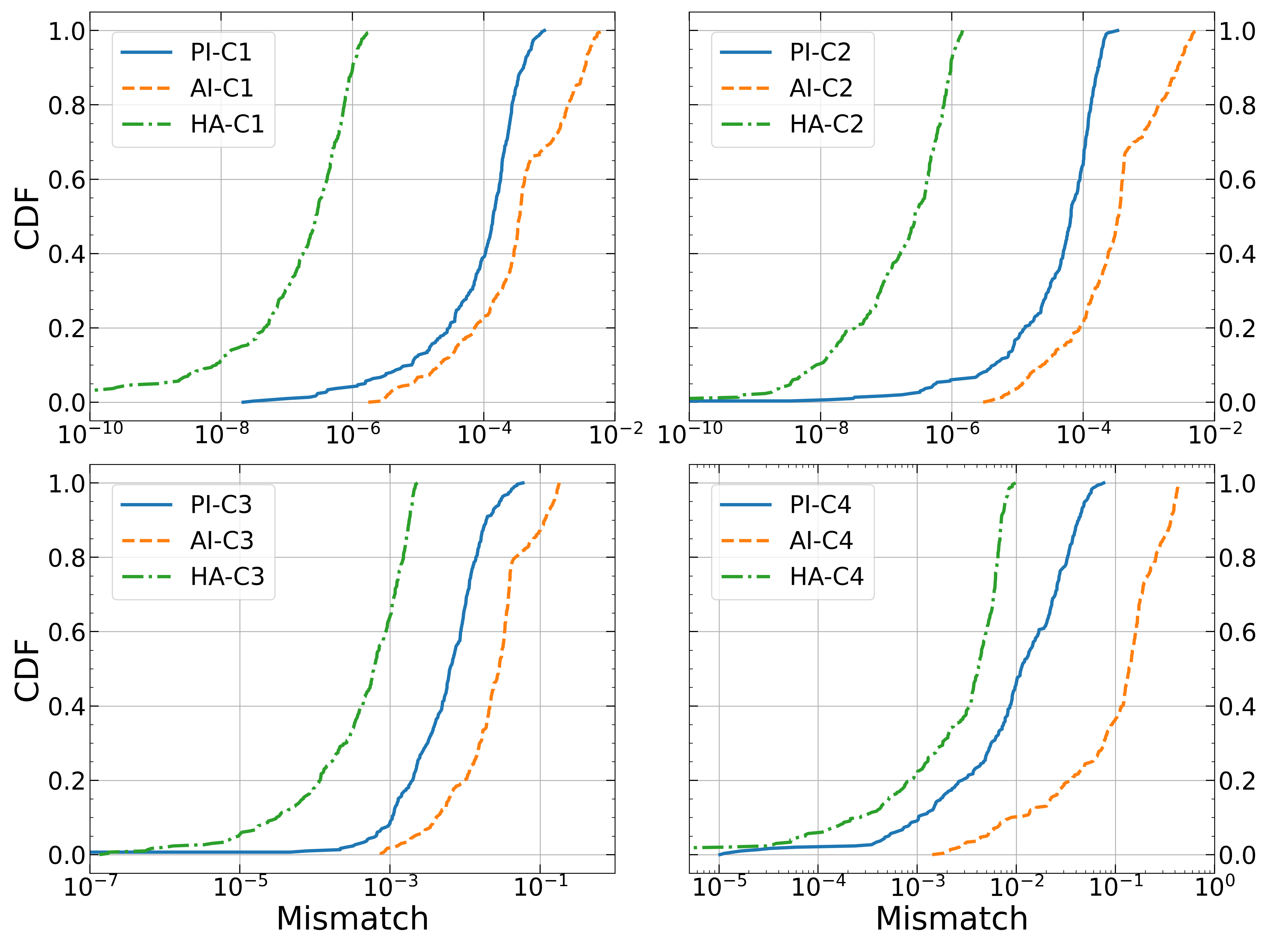
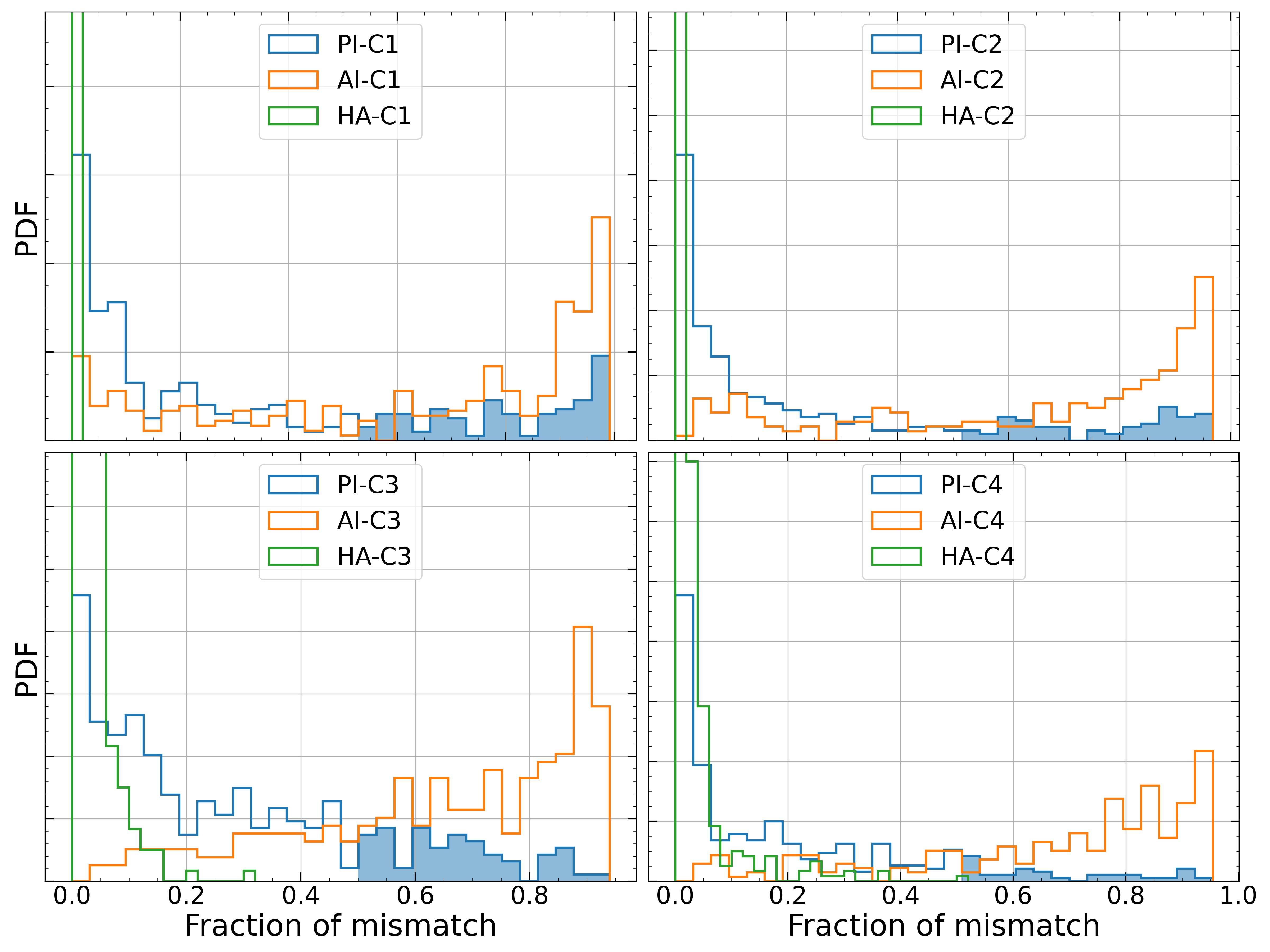
Figure 1: Left: the CDF of each effect for 4 different cases. PI is an abbreviation for Precession Induced, AI refers to Aligned-spin Induced while HA is Horizon Absorption effect. The $Mismatch$es of C1 and C2 are two order of magnitudes smaller than C3 and C4 because their mass ratios ($q=m_{1}/m_{2}>1$) are much greater than C3 and C4. Right: the distribution of fraction of mismatch defined in Eq. 11 of each effect for 4 cases. The histogram is normalized for individual effects. We could see the shaded areas which demonstrate the fraction of samples with more than $50\%$ mismatch contribution from the PI effect are about $31\%\,,23\%\,,21\%$ and $14\%$ for cases C1 to C4, respectively.

The left panel of Fig. 1 shows that, for all four cases, the black hole horizon absorption effect produces the least mismatch and the aligned spin induced quadrupole moment leads to the highest overall mismatch. The right panel, on the other hand, compares the fraction of mismatch as defined by

$$F_{i}:=\frac{\mathcal{M}_{i}}{\mathcal{M}_{\rm PI}+\mathcal{M}_{\rm AI}+\mathcal{M}_{\rm HA}},\quad i={\rm PI,AI,HA}$$ (11)

The precession SIQM is the dominant mechanism for producing mismatch for approximately $20\%$ of the spin configurations, where spin precession is significant.

The mismatch due to horizon absorption is consistent with the analysis in [69, 70], where the phase modulation due to the horizon absorption effect is shown to be extremely small. Comparisons can also be made between the mismatch of different cases. For example, for the precession SIQM-induced mismatch, the values for “C1” binaries are generally larger than those of “C2” binaries, because of the larger spin assumed for object one in C1. The mismatch also seems to be higher for comparable mass-ratio systems, as the magnitude of mismatch of “C3” binaries is significantly higher than “C1” binaries. In the first three cases, this is due to the fact that the effect of the SIQM on the waveform is suppressed by the mass ratio, since only the smaller object has $\kappa\neq 1$. In the fourth case, since both objects have $\kappa\neq 1$ the effect is large, regardless of mass ratio since the large object’s effect is not suppressed by the mass ratio. If the binary contains a normal neutron star, such as the “C4” binaries, the associated $\kappa$ may be significantly greater than that of the mass-gap objects [25]. Although the underlying spin of the neutron star is assumed to be small $\chi_{2}=0.05$, the resulting mismatch is still mostly in the range between $10^{-2}$ to $10^{-1}$.

While the mismatch is informative for comparing effects very roughly, the Mismatch study alone is not able to provide quantitative measures on the measurement accuracy of $\kappa$ across the different scenarios. In the next section we use the Bayesian Inference method, together with MCMC parameter estimation to obtain posterior distribution of system parameters, including $\kappa$, for selected sets of scenarios. This task can not be done simultaneously for all spin configurations shown in Fig. 1 because of the large computational cost associated with these MC simulations. In order to pick the most representative cases, we adopt the median mismatch configurations from the CDF plots as injected system parameters to perform the Bayesian inference.

As we will show in Sec. II.4.1, having the same level of mismatch does not necessarily imply the same level of measurement uncertainty of $\kappa$, as we will see in the MCMC simulations. Although the mismatch contribution from non-precessing SIQM is significantly greater than precessing SIQM for all four types of systems, the MCMC simulations actually show that the posterior distribution of $\kappa$ is more sensitively determined by the precessing SIQM rather than the non-precessing SIQM, even if their corresponding mismatch is comparable. For almost all cases where the spin precession is significant, the contribution to the posterior distribution of $\kappa$ from non-precessing SIQM is smaller than the precessing SIQM effect. As a result, later on when we pick sample spin configurations to estimate the measurement uncertainty of $\kappa$, we select the median mismatch configurations from the PI effect alone.

II.3 Parameter Estimation

In order to compute the measurement uncertainty, we shall apply the Bayesian inference method [71, 72], which is developed based on MCMC and Bayes’ theorem. According to the Bayes’ theorem, given GW data $d$ and hypothesis $\mathcal{H}$, the posterior distribution $p(\mathcal{\bm{\vartheta}}|d,\mathcal{H})$ is given by

$$p(\mathcal{\bm{\vartheta}}|d,\mathcal{H})=\frac{p(d|\bm{\vartheta},\mathcal{H})\;p(\bm{\vartheta}|\mathcal{H})}{p(d|\mathcal{H})}=\frac{p(d|\bm{\vartheta},\mathcal{H})\;p(\bm{\vartheta}|\mathcal{H})}{\int d\bm{\vartheta}\;p(d|\bm{\vartheta},\mathcal{H})\;p(\bm{\vartheta}|\mathcal{H})}\,.$$ (12)

Here $p(d|\bm{\vartheta},\mathcal{H})$ is the likelihood function while $p(\bm{\vartheta}|\mathcal{H})$ is the prior on $\mathcal{\bm{\vartheta}}$. Assuming a stationary Gaussian noise, the log likelihood function $\log p(d|\bm{\vartheta},\mathcal{H})$ can be expressed as

$$\log p(d|\bm{\vartheta},\mathcal{H})=\log\bar{\alpha}-\frac{1}{2}\sum_{k}\left<d_{k}-h_{k}(\bm{\vartheta})|d_{k}-h_{k}(\bm{\vartheta})\right>\,,$$ (13)

where the index $k$ refers to different detectors and $\log\bar{\alpha}$ is the normalization factor while $d_{k}$ and $h_{k}(\bm{\vartheta})$ are the data and waveform templates from given detectors.

As explained in Sec. II.2, we shall compute the posterior distributions for selected parameter configurations for all four cases displayed in Fig. 1. Among the randomized spin configurations and orbital inclinations in Fig. 1, we choose the ones corresponding to the median value of PI mismatch in each category since the contribution to the measurement accuracy of $\kappa$ from the AI effect is much weaker than the PI effect, even though this would not be clear from their relative mismatches (see Sec. II.4.1). The relevant system parameters are shown in Table 2, with the rest of parameters consistent with Table 1. Notice that for each setup, there are 16 or 17 binary parameters in total depending on whether $\kappa$ from the non-$2.6M_{\odot}$ object is included or not. For all configurations the luminosity distance is set to be $d_{\mathrm{L}}=200$ Mpc, sky location is fixed as $(\alpha,\delta)=(1.0,2.0)$ and polarization angle $\psi=3.0$. The coalescence phase and coalescence time are chosen randomly, since they have almost no influence on the simulation results.

We employ LALSuite [60] and PyCBC [73] packages with specific modifications to generate waveforms and run MCMCs. Regarding to the MCMC configurations, we adopt the $marginalized\_polarization$ likelihood model developed by PyCBC group. This model numerically marginalizes over polarization angle which will reduce one prior parameter. A modified version of $rwalk$ named $rwalk2$ method is chosen to sample the prior space. Other important setups are: $nlive=5000$, $dlogz=0.1$ and burn-in test is $nacl\;\&\;max\_posterior$. A low frequency cutoff $f_{\rm low}=20$ Hz is set for all simulations and we always set a uniform prior on $\kappa$ with a range which doesn’t affect the results. In addition, all the injected signals are generated with the same waveform model as the MCMC realization unless stated differently.

		C1	C2	C3	C4
$\theta_{1}$		1.05	2.37	1.07	1.43
$\theta_{2}$		1.13	2.63	2.25	0.35
$\phi_{1}$		0.51	0.91	2.50	5.73
$\phi_{2}$		0.77	4.70	1.01	2.09
$\iota$		1.43	1.15	1.49	2.52
SNR	A#	122	97	27	61
	CE	1568	1401	250	736

Table 2: Parameters corresponding to the median value of PI mismatch for MCMCs. $\theta_{i}$ and $\phi_{i}$ are the polar and azimuthal angles, respectively. $\iota$ refers to the inclination angle. The last two rows show the optimal SNRs for different detector networks.

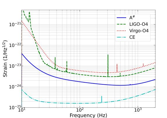
Figure 2: Sensitivity curves of LIGO-O4, Virgo-O4 [74], A^# [75] and CE [76] detectors.

We would like to assess the detectability of the SIQM in different eras of detector development. For this purpose, we have assumed two sample detector networks. The first we have dubbed the A^# network, and consists of four detectors with A^# sensitivity located at Hanford, Livingston, LIGO India, Virgo and KAGRA, respectively. The LIGO detectors have started the O$4$ observing run with expected duration of $18$ months. There will be a following O$5$ observing run scheduled for late 2020s, and a post-O$5$ upgrade - the A^# detector using the same LIGO facility. This first sample detector network is intended to show the constraining power of such a detector network. The other sample detector network, dubbed the cosmic explorer (CE) network here, consists of three detectors with CE sensitivity located at Hanford, Livingston, and LIGO India, respectively. This is chosen to represent the constraining capability of a network of third generation ground-based detectors; leading concepts for which are the US-led detector Cosmic Explorer [77, 78] and European-led detector Einstein Telescope [79, 80], of which we have chosen CE for simplicity as a representative third generation detector. The corresponding sensitivity curves for various detectors are shown in Fig. 2.

In Table 2, we display the event SNR (signal-to-noise ratio) for each case, assuming the A^# network and the CE network respectively. The optimal matched filter SNR $\rho_{\rm opt}$ is defined as

$$\rho_{\rm opt}=\sqrt{\sum_{k}<h_{k}|h_{k}>}=\sqrt{4\sum_{k}\int_{f_{\rm low}}^{f_{\rm high}}\frac{\tilde{h_{k}}^{*}(f)\tilde{h_{k}}(f)}{S_{n,k}(f)}df}\,,$$ (14)

where the index $k$ refers to the $k$th detector and $h_{k}$ is the GW strain obtained at the $k$th detector. C1 and C2 cases have higher SNR because they have larger chirp mass for the binaries. The SNR is also sensitive to the inclination angle of the orbital plane.

II.4 Simulation Results

II.4.1 Significance of different effects

In order to study the impact of the PI and AI effect in constraining $\kappa$, we consider a GW190814-like event (C2) as a sample system (as shown in Table 1 and 2) to perform MCMC simulations. The injected waveform (modified IMRPhenomXPHM) includes all the effects (PI, AI and HA). Notice that this C2 system already contains significant spin precession, and we choose to use waveforms with the PI or the AI effect for parameter estimation. For completeness, we also include a MCMC study with the TaylorF2 waveform commonly used for aligned-spin systems. For this case, the injected values for the aligned spins $\chi_{1z}$ and $\chi_{2z}$ are assumed to be the same as the magnitude of spins $\chi_{1}$ and $\chi_{2}$ in the precessing case.

For waveforms including only non-precessing SIQM effects, it is known that there is a degeneracy between the $\kappa$ and spins $\chi_{1z}$ and $\chi_{2z}$ [25]. We illustrate this point with a simulation (GW190814-like event (like C2) with A^# network) using the TaylorF2 waveform model. The result is shown in the left panel of Fig. 3 with a clear degeneracy observed between $\kappa$ and the spin parameters, which generally degrades the measurement accuracy of $\kappa$. This degeneracy is no longer present for precessing systems as shown in the right panel of Fig. 3. However, even if there is no degeneracy, it seems that the precessing waveform model including only the AI effect has poor measurement accuracy on $\kappa$. In Fig. 3, we also present the posterior distribution of parameters with the PI effect included in the waveform model. We find that the constraint on $\kappa$ becomes much tighter. Notice that the underlying spin configuration is chosen such that the relative contribution to the total mismatch from PI and AI effects is roughly $50\%:50\%$. The result shows that for the same level of mismatch, PI effects tend to have much better correlation with the measurement uncertainty of $\kappa$. Therefore, when we pick a sample binary parameter to estimate the “typical” measurement uncertainty of $\kappa$ for different types of systems and for different spin configurations, it should be more appropriate to choose injected waveform parameters (shown in Table 2) with a median value of mismatch for the PI effect alone (because it is more relevant for the $\kappa$ uncertainty) rather than the total mismatch as shown in Fig. 1.

In addition, for binaries with two non-black hole objects, it is noted in [25] that the degeneracy between $\kappa_{1}$ and $\kappa_{2}$ severely compromises the possibility of individually measuring $\kappa_{1,2}$. Including higher PN correction terms does not significantly improve the situation. We find that the $\kappa$ for both mass-gap objects (C3) can be individually measured without being affected by degeneracies, thanks to the precessing SIQM effect and the relatively high spin magnitude ($\sim 0.7$) assumed for the mass-gap objects.

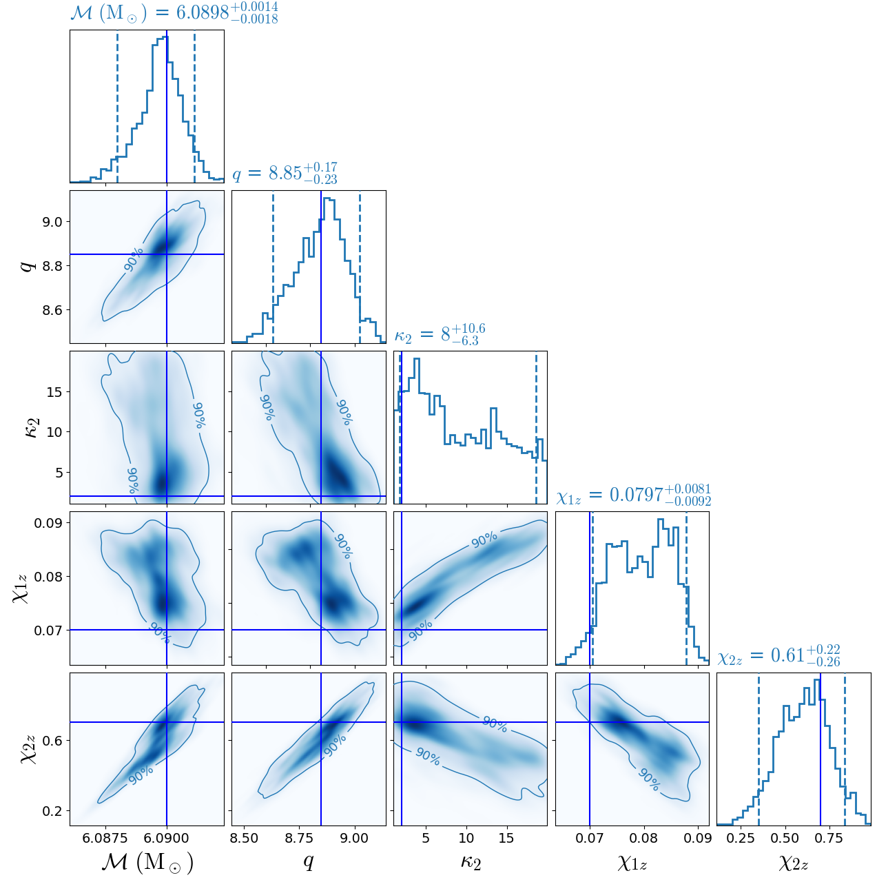
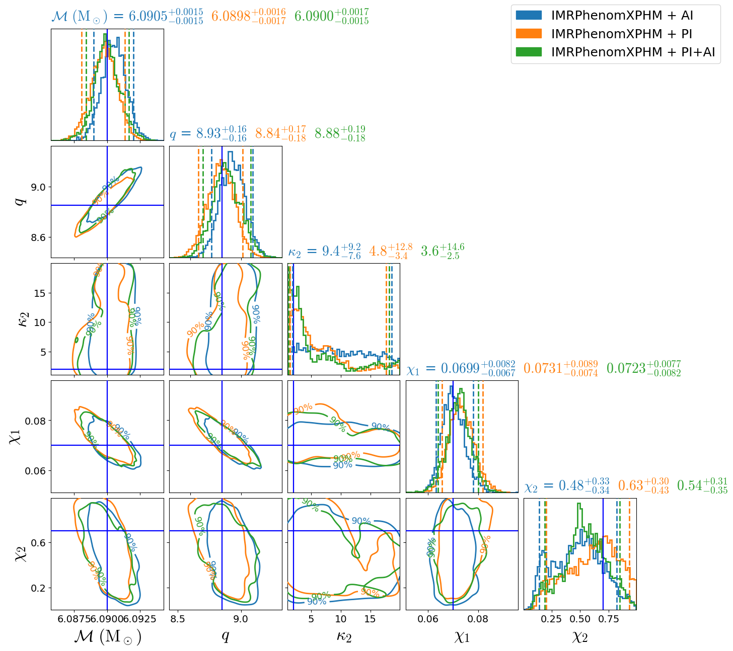
Figure 3: Left: a corner plot shows the degeneracy between SIQM $\kappa$ and spins $\chi_{1z}$ and $\chi_{2z}$ with TaylorF2 waveform model. Right: a comparison between AI, PI or PI+AI effects in precessional waveform models with the same injection while the fractional mismatch of PI is close to AI with $\approx 50\%$ of the total mismatch (Note that there is no PI effect in TaylorF2 waveform model and we assumed an aligned spins in the left plot). The dashed lines in marginalized distributions are the $5\%$ and $95\%$ credible level lines.

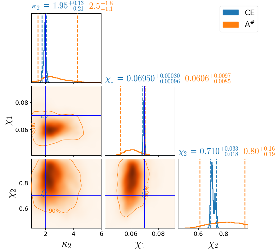
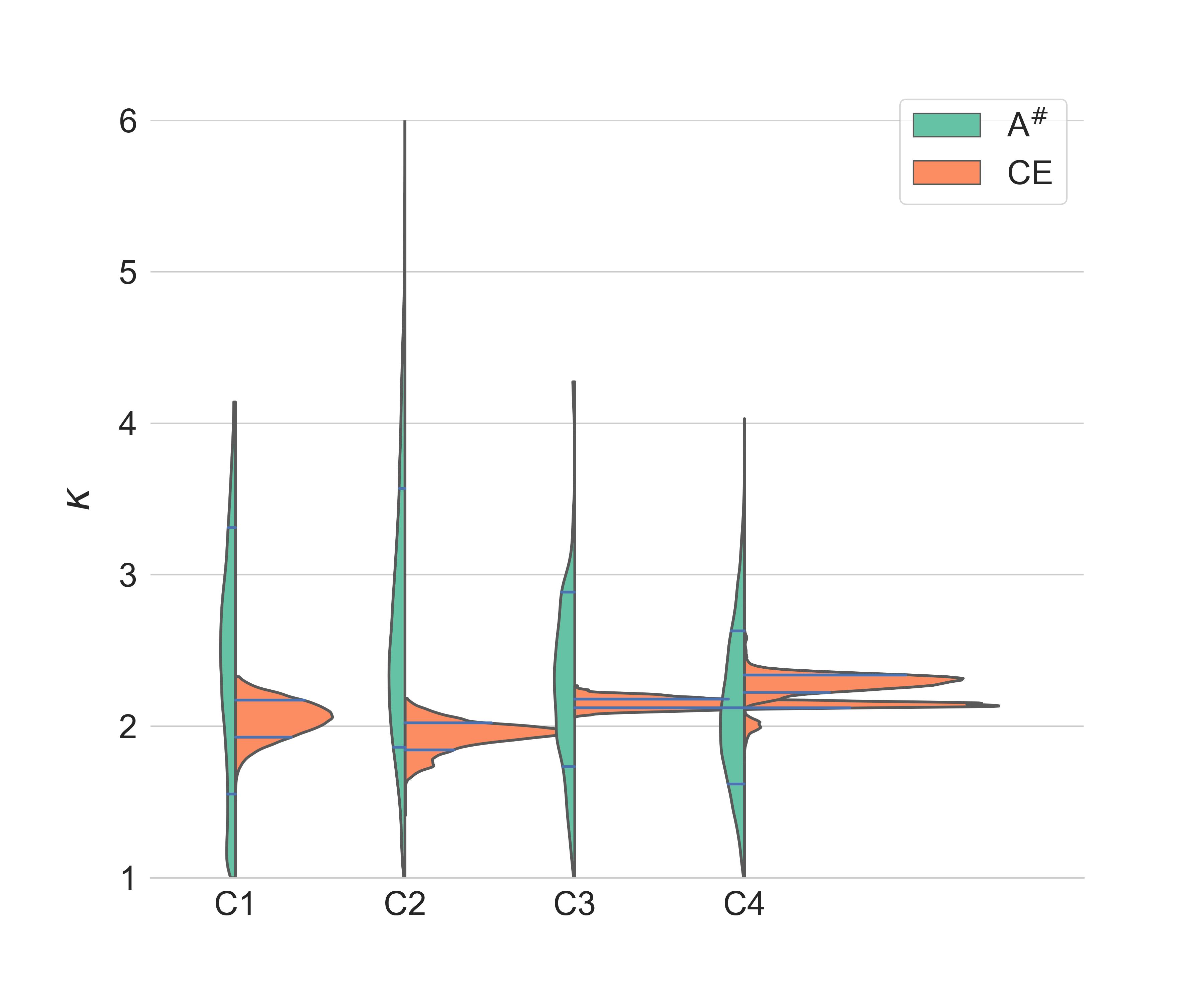
Figure 4: Left: posterior distribution of SIQM $\kappa_{2}$, $\chi_{1}$ and $\chi_{2}$ with A^# and CE networks, respectively. Here the range of values above the marginalized distributions are given within a $90\%$ confidence interval. Right: violin plot for $\kappa$ of the $2.6\,M_{\odot}$ object for the four cases. The violin has been split into two parts: green (left) and orange (right) present constraints from the A^# and CE networks. Each half violin has the same area and the horizontal lines show 1 $\sigma$ uncertainty bounds.

II.4.2 Results for Four Types of Sources

In order to assess the measurement uncertainty of $\kappa$ for mass-gap objects with future GW observations, we consider different types of systems with different detector networks as shown in Table 1 and 2. Notice that we have assumed the same distance for all systems in Table 1 and 2, whereas in reality the expected distance of different types of systems may vary, depending on the underlying merger rate. For a binary at a different distance, one can easily scale the uncertainty as the measurement SNR is inversely proportional to the distance.

For example, with the modified IMRPhenomXPHM waveform that includes both precessing and non-precessing SIQM effects and the possible horizon absorption effect, the posterior distribution of relevant binary parameters of the “C2” scenario in Table 2 is shown in the left panel of Fig. 4. For a GW190814-like event (like C2) with low primary spin, assuming the A^# network, the measurement uncertainty of $\kappa_{2}$ is around 2 with a $90\%$ upper limit placed at $\kappa\approx 3.9$. On the other hand, the CE network gives rise to a measurement of $\kappa_{2}=1.95_{-0.21}^{+0.13}$, which means that the third-generation detector will be able to provide decisive evidence on the nature of the mass-gap objects, assuming they are rapidly spinning.

In the violin plot shown in Fig. 4, we summarize the posterior distribution of $\kappa$ of the $2.6\,M_{\odot}$ object from MCMC simulations corresponding to different detector networks and binary cases. It is evident that with the assumed system parameters, the A^# network is only capable of marginally constraining the nature of the mass-gap objects, as the $\kappa=1$ case cannot be excluded with high statistical significance. While the PI mismatch of “C3”- and “C4”-type binaries is about two order of magnitude greater than “C1”- and “C2”-type binaries (as the mass ratios for C3 and C4 are much smaller than fror C1 and C2), the constraints on $\kappa$ of the $2.6M_{\odot}$ object are within the same order of magnitude for all four cases. This is because in C3 and C4 both objects have $\kappa$ as a free parameter, whereas only the less massive object in C1 and C2 has an undetermined $\kappa$. The CE network should be able to draw decisive conclusions for all four binaries considered.

III Black hole mimickers

Black hole mimickers may be star-like objects (e.g. boson stars [45, 46]) with continuous matter/field distribution, or contain hard boundaries (e.g. gravastars [47, 48, 49] and AdS bubbles [51]) that separate out different spacetime regimes. In addition, alternative black hole solutions predicted by modified theories of gravity may also be classified as black hole mimickers. In order to test/constrain their existence, it is useful to examine several key observables from the gravitational wave measurements such as the tidal Love number, the SIQM, and absorption/additional dissipation effects [81]. Current models of boson stars could produce a $\kappa$ ranging from 10 to 150 [45, 34, 35, 36]. In the future, if there are events with statistically significant $\kappa\neq 1$ from heavy objects (such that these objects cannot be neutron stars), it will provide evidence for the existence of exotic objects.

In this section, we focus on the scope of measuring SIQMs of black hole mimickers including both precessing and non-precessing effects. Since such an analysis has been performed for binary black hole events in the GWTC-$1$ [53], GWTC-$2$ [54] and GWTC-$3$ [55] catalogs considering only the non-precessing SIQM effect, we first re-perform the analysis for a few events with clear signature of spin effects, with the precessing SIQM considered. In addition, we will discuss the prospects of such measurement for O$4$ binaries, and show that it is possible to obtain better constraints on the SIQMs.

One important difference for the MC simulations performed in this section is that instead of having individual $\kappa$ for the two objects in the binary, we assume that $\kappa_{1}$=$\kappa_{2}$ (following the convention in [55]) and define the symmetric SIQM and its deviation from 1:

$$\kappa_{s}=(\kappa_{1}+\kappa_{2})/2\,,\quad\delta\kappa_{s}=\kappa_{s}-1\,.$$ (15)

For black hole binaries, $\delta\kappa_{s}=0$. A non-zero value of $\delta\kappa_{s}$ with sufficient statistical significance would indicate the object is not a black hole (at least, not the kind in GR).

III.1 GWTC Events

The constraints of $\delta\kappa_{s}$ from individual GW events have been discussed in the LVK Collaboration paper [53, 54, 55] with GWTC events using the IMRPhenomPv2 waveform model [82]. This waveform model is different from the IMRPhenomXPHM waveform model in the following ways: First, it is based on the next-to-next-to-leading order single-spin PN approximation [83] while IMRPhenomXPHM is based on the double-spin MSA approach [84] when twisting up the aligned-spin waveform modes in the co-precessing $L$-frame to the inertial $J$-frame. Second, it uses a non-spinning 2PN approximation to the orbital angular momentum, while IMRPhenomXPHM uses an aligned-spin 4PN approximation including spin-orbit contributions. The MSA approach performs much better as an approximation to the Euler angles as shown in Fig. 3 of [57]. Finally, IMRPhenomPv2 does not include higher order multipoles.

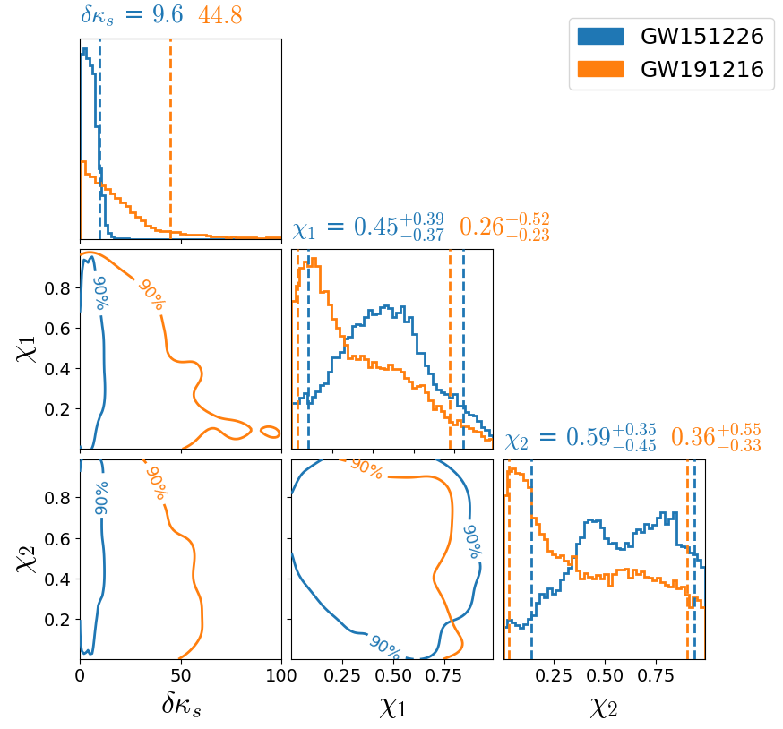
Figure 5: Posterior distribution of quadrupole moment deviations $\delta\kappa_{s}$, $\chi_{1}$ and $\chi_{2}$ from GW events with the IMRPhenomPv2 waveform model. The dashed lines in marginalized $\delta\kappa_{s}$ are the $90\%$ upper bound, while they are the $5\%$ and $95\%$ credible level lines for $\chi_{1}$ and $\chi_{2}$.

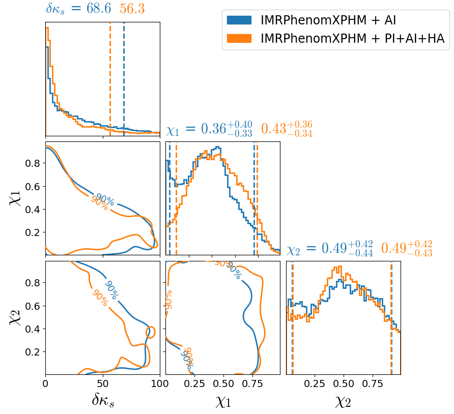
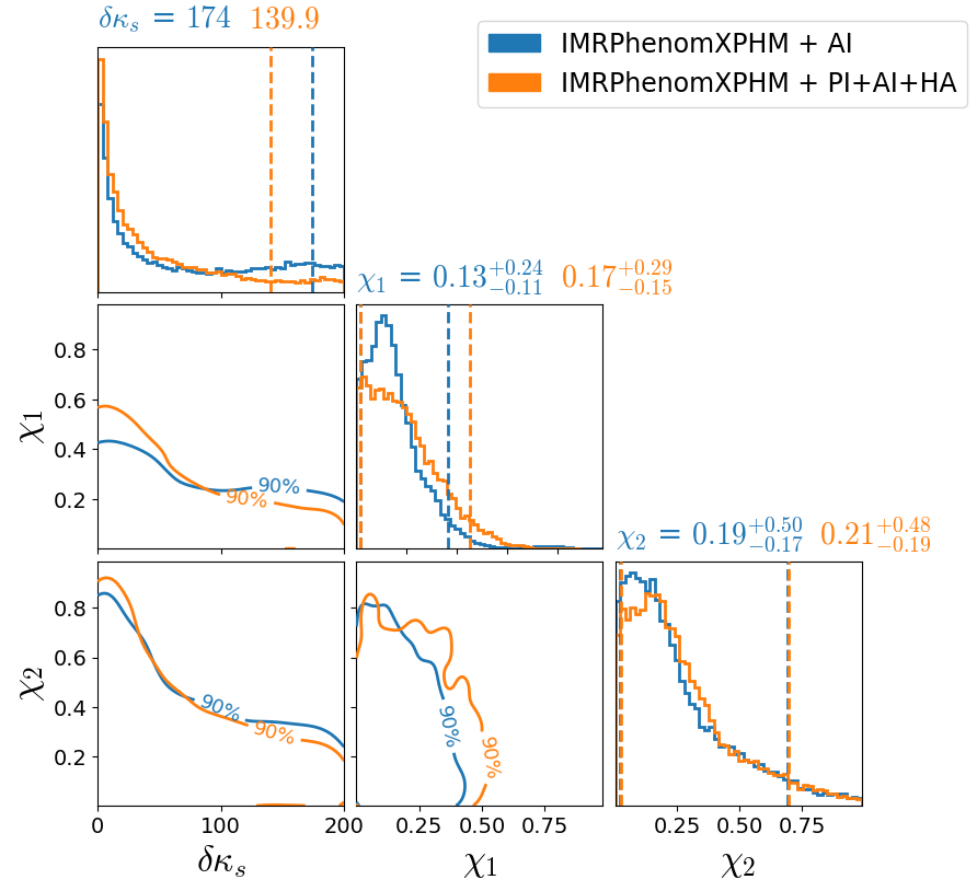
Figure 6: Posterior distribution of quadrupole moment deviations $\delta\kappa_{s}$, $\chi_{1}$ and $\chi_{2}$ with GW151226 (left) and GW191216_213338 (right) with the IMRPhenomXPHM + different effect combination. The dashed lines in marginalized $\delta\kappa_{s}$ are $90\%$ upper bound, while they are $5\%$ and $95\%$ credible level lines for $\chi_{1}$ and $\chi_{2}$.

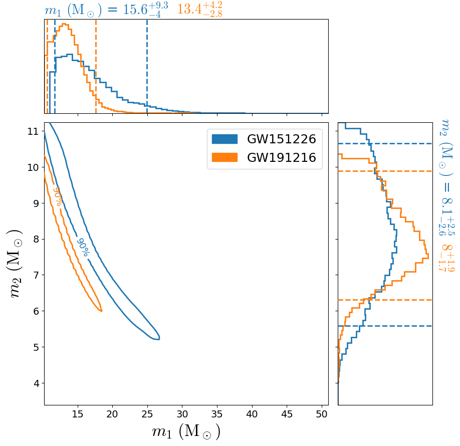
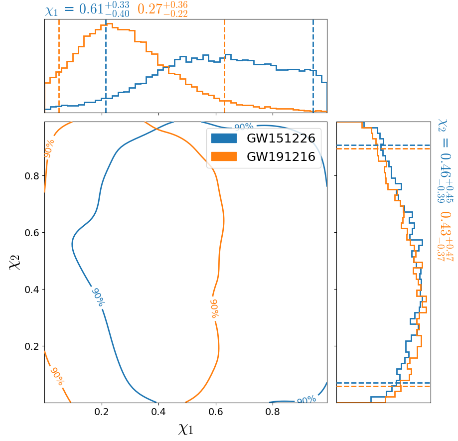
Figure 7: Posterior distribution of individual masses and spins with GW151226 and GW191216_213338. The dashed lines in marginalized plots are $5\%$ and $95\%$ credible level lines. The posterior samples used in this plot are from public available works [85].

To further illustrate the difference between the two waveform models, we choose GW events GW151226 and GW191216_213338 (downloaded from The Gravitational Wave Open Science Center (GWOSC) [86]), which show nonzero spins in the posterior and perform MC parameter estimation using IMRPhenomPv2 versus IMRPhenomXPHM ($l=m=2$ mode only). The resulting posterior distribution of $\delta\kappa_{s}$ is shown in Fig. 5 and Fig. 6, respectively. We find that the IMRPhenomPv2 waveform generally leads to much tighter constraints than the IMRPhenomXPHM waveform, which is counter-intuitive as by construction the IMRPhenomXPHM waveform describes the spin dynamics more accurately than the IMRPhenomPv2 waveform. We think that the discrepancy comes from the fact that the IMRPhenomPv2 waveform contains much larger phase error than the IMRPhenomXPHM waveform when $\delta\kappa_{s}$ is large, so that the large $\delta\kappa_{s}$ regime is more easily ruled out for the IMRPhenomPv2 waveform. Therefore, a more accurate waveform does not always lead to tighter constaints on $\delta\kappa_{s}$, at least in the relatively low SNR limit. In the high SNR limit, on the other hand, we expect that the systematic error in the IMRPhenomPv2 waveform shall lead to a more biased measurement of $\delta\kappa_{s}$. We will further compare these two waveforms with the injected event in the next section.

In addition, when we use the IMRPhenomPv2 waveform for parameter estimation for GW151226 and GW191216_213338, we obtain the $90\%$ constraints on $\delta k_{s}$ to be $\sim 10$ for GW151226 and $\sim 40$ for GW191216_213338. The former result is consistent with the bound listed in [54], but the latter is about four times greater than the bound presented in [55], which is also $\sim 10$. However, as we compare the binary parameters, the component masses and the SNRs for these two events are similar, but the inferred spins of GW151226 are significantly larger than those of GW191216_213338 (see the comparison in Fig. 7). Therefore, one would expect tighter constraints on $\delta\kappa_{s}$ for GW151226. In fact, when we use the IMRPhenomXPHM waveform for parameter estimation, we indeed also find that the constraint from GW151226 is tighter than that from GW191216_213338 as shown in Fig. 6.

The IMRPhenomXPHM waveform model with the precessing SIQM effect included provides more accurate spin dynamics, and potentially more constraining power on $\delta\kappa_{s}$ because the precessional SIQM effect tends to introduce additional mismatch in the waveform for precessing binaries. For GW151226 and GW191216_213338, the resulting posterior distributions of spin parameters are shown in Fig. 6 in comparison with those without the precessing SIQM. For both events, we only observe marginal improvement in constraining $\delta\kappa_{s}$: for GW191216_213338 the $90\%$ confidence interval of $\delta\kappa_{s}$ with PI effect included is $\sim 140$ and without PI is $\sim 174$; for GW151226 the $90\%$ confidence interval of $\delta\kappa_{s}$ with PI effect included is $\sim 56$ and without PI is $\sim 68$. The improvement is not very significant, potentially because the spin precession in both system are still mild.

III.2 Injected Events

In order to further compare the performance of the IMRPhenomPv2 waveform and the IMRPhenomXPHM waveform ($l=m=2$ mode only and without the PI effect included yet) in constraining $\delta\kappa_{s}$, we inject a GW151226-like event (with detailed parameters shown in Table 3) using the IMRPhenomXPHM waveform, and try to recover the parameters using both waveforms. The posterior distributions are shown in Fig. 9 (left panel). We find that although the underlying event is generated by the IMRPhenomXPHM waveform, the posterior distribution of $\delta\kappa_{s}$ is actually much tighter if we use the IMRPhenomPv2 waveform for recovery (except for the far tail points, which are responsible for the larger 90$\%$ upper bound). The reason is that the IMRPhenomPv2 waveform produces much larger mismatch for large $\delta\kappa_{s}$, so it appears to be more constraining than the more accurate waveform. In general, as we compute the mismatch between the $\delta\kappa_{s}=0$ waveform and a $\delta\kappa_{s}\neq 0$ waveform, the true waveform should have its mismatch depend on $\delta\kappa_{s}$ with one particular function dependence, but the inaccurate waveforms may have their mismatch larger or smaller than the true mismatch for the same $\delta\kappa_{s}$. If the mismatch of the inaccurate waveform is larger than the true mismatch, it will appear to be more constraining than the true waveform, and vice versa. This is illustrated in Fig. 8.

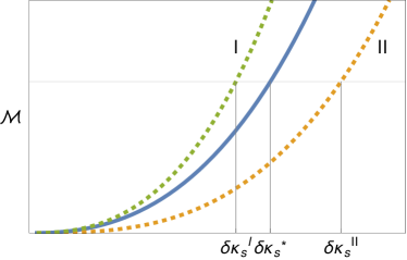
Figure 8: This cartoon plot illustrates that a more accurate waveform model does not necessarily imply better constraints on $\delta\kappa_{s}$ (This plot is for illustration purpose only, which is not computed out of an actual calculation. We assume the mismatches reduce to zero as $\delta\kappa_{s}\to 0$, in other words, they reduce to the same waveform models as $\delta\kappa_{s}\to 0$). Three different waveform models are shown: the true waveform in solid blue, and two alternative waveform models in dashed (green is labelled I, and yellow labeled II). For a given mismatch, the true waveform model will be able to constrain $\delta\kappa_{s}^{\star}$ to $\left[0,\delta\kappa_{s}\right]$. The incorrect waveform model II will give a poorer constraint, as the range $\left[0,\delta\kappa_{s}^{\rm II}\right]$ is larger than $\left[0,\delta\kappa_{s}^{\star}\right]$. However, the incorrect model I will give a tighter constraint.

We can also use injected events to compare the performance of IMRPhenomXPHM waveforms with or without the precessional SIQM effect included. To do this, we construct an O4-type network (LIGO Hanford, LIGO Livingston and Virgo) to test one case of BH mimickers. The binary configuration we assume is shown in Table 3, with one of the black holes having a significant spin magnitude $\chi_{1}=0.5$, and the spin of the other black hole is small $\chi_{2}=0.05$. With the assumed distance at $200$ Mpc, the network SNR is approximately 110. Notice that if a similar system is detected at a different distance, one can scale the uncertainties accordingly, as the SNR is inversely proportional to the distance. For the injected waveform, we also assume that these are two BHs with $\kappa_{1}=\kappa_{2}=1$, hence $\delta\kappa_{s}=0$. Among the randomly generated spin orientation and inclination angles, we pick a set of parameters such that the mismatch contribution from the PI and AI effect are also roughly $50\%:50\%$, so that we can assess the constraining power of the PI effect relative to the AI effect, since based on mismatch alone they should contribute evenly.

In the Fig. 9 (right panel), we present the posterior distribution of $\delta\kappa_{s}$ and the dimensionless spin magnitudes. With the PI effect included, there is a much tighter constraint on the magnitude of $\delta\kappa_{s}$. In addition, the measurement uncertainty on $\chi_{2}$ (the spin of the slowly-rotating black hole) also becomes significantly better than the distribution recovered without using the PI effect. Although we have not made further comparison using more simulated data in different scenarios, it is reasonable to expect that the waveform model with the PI effect included will improve the measurement of $\delta\kappa_{s}$ for at least some of the O4 events. Even if it did not offer significant additional constraining power, physically the PI effect is present if $\delta\kappa_{s}$ is nonzero and the system is precessing. To produce results as accurately as possible and without bias, we should apply the more complete waveform model, since there is little additional computational overhead associated in doing so [57].

	$(m_{1},m_{2})(M_{\odot})$	$(\kappa_{1},\kappa_{2})$	$(\chi_{1},\chi_{2})$	$(\theta_{1},\theta_{2})$	$(\phi_{1},\phi_{2})$	$\iota$	$(\alpha,\delta)$	$d_{\mathrm{L}}$(Mpc)	SNR
C5	(16, 8)	(1, 1)	(0.6, 0.5)	(1.0, 1.4)	(3.2, 3.1)	1.3	(3.5, -0.2)	490	15.5(aLIGO)
C6	(30, 20)	(1, 1)	(0.5, 0.05)	(1.02, 0.5)	(6.26, 2.49)	2.46	(1, 2)	200	110(O4), 443((A#)

Table 3: Configurations of two BBH injections used for MCMC simulations, where C5 is a GW151226-like injection. The last column shows SNRs for the GW151226-like event, which is close to the real event SNR, and for C6 with O4 network and A^# sensitivity, respectively.

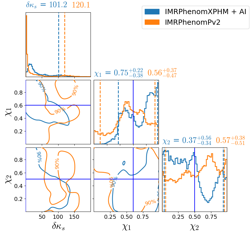
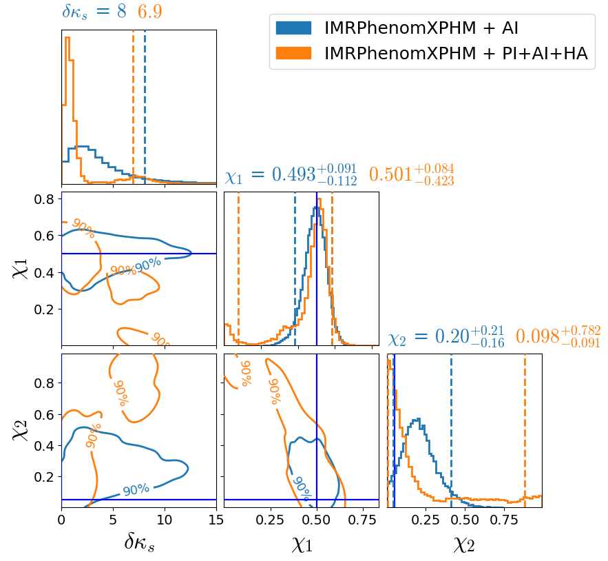
Figure 9: Posterior distribution of quadrupole moment deviations $\delta\kappa_{s}$, $\chi_{1}$ and $\chi_{2}$. Left: result from C5 (GW151226-like) injection with IMRPhenomXPHM+AI but recovery with IMRPhenomXPHM+AI and IMRPhenomPv2 models. Right: C6 with O4 detector network. The dashed lines in marginalized $\delta\kappa_{s}$ are $90\%$ upper bound, while they are $5\%$ and $95\%$ credible level lines for $\chi_{1}$ and $\chi_{2}$.

IV Conclusions

We have examined the effect of the SIQM on the resulting waveform, and the constraints that can be placed on the SIQM of objects as a result. We have shown that, at least for some precessing configurations, by including the effect of the SIQM on the precession description of spins and angular momentum, it is possible to achieve better measurement accuracy on $\kappa$. This has important consequences in assessing the nature of mass gap objects where other methods, namely the tidal deformability, horizon absorption (or lack thereof), and EM counterpart, may fail to distinguish between the heavy neutron stars and light black holes.

In our analysis, we used the waveform model that includes the complete SIQM effect [33] and run MCMC simulations. We find that for another GW190814-like event, with an A^# type detector network, the statistical significance for individual events is generally not sufficient to distinguish between the nature of objects with high confidence. However, for a CE network we should easily be able to distinguish between neutron stars and black holes for such mass-gap objects.

Second, we find that, using this waveform model, even with O4 sensitivity we can place tighter constraints than similar waveform models that ignore this effect. This is a result of the precession effect influencing the constraining power more than the aligned-spin effect. This, of course, with the caveat that the system must be exhibiting significant precession. On the other hand, through the illustration with injected events and real events from the GWTC catalog, we have shown that a more accurate waveform does not necessarily lead to tighter constraints on $\delta\kappa_{s}$ for the tests of black-hole mimickers. Fortunately, with the state-of-the-art IMRPhenomXPHM waveform, it appears that by including the precessional SIQM effect the waveform becomes both more accurate and more constraining in determining $\delta\kappa_{s}$.

To reiterate on our previous work, one potential avenue of improvement is improving the computational efficiency by producing a more analytic solution to the spin-dynamics. Another potential addition to the waveform in the future is the inclusion of eccentricity. Since eccentricity and precession can produce similar effects on the waveform, not including eccentricity in the waveform model can produce posteriors that entirely exclude the true system parameters.

Appendix A Posterior distributions of spin polar angles of GW151226 and GW191216_213338

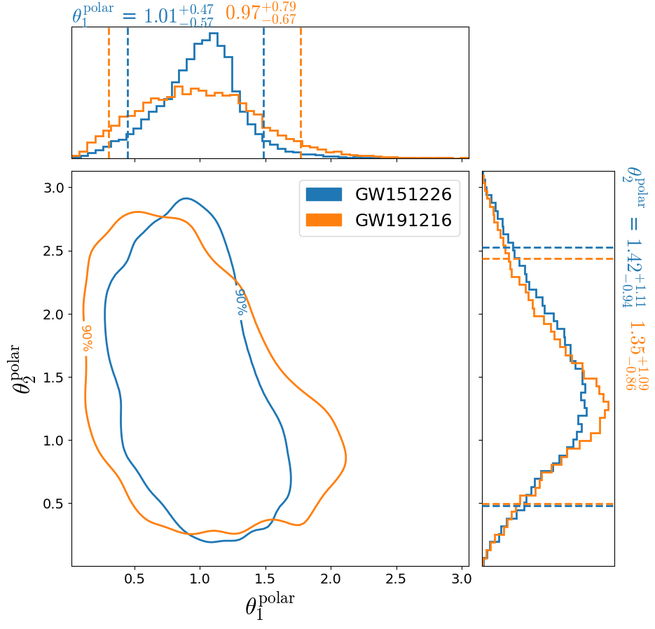
Figure 10: Posterior distribution of individual spin polar angles with GW151226 and GW191216_213338. The dashed lines in marginalized plots are $5\%$ and $95\%$ credible level lines. The posterior samples used in this plot are from public available works [85].

References

- [1] B. P. Abbott, R. Abbott, T. D. Abbott, S. Abraham, F. Acernese, K. Ackley, C. Adams, R. X. Adhikari, V. B. Adya, C. Affeldt, and Agathos. Gwtc-1: A gravitational-wave transient catalog of compact binary mergers observed by ligo and virgo during the first and second observing runs. Phys. Rev. X, 9:031040, Sep 2019.
- [2] R. Abbott, T. D. Abbott, S. Abraham, F. Acernese, K. Ackley, A. Adams, C. Adams, R. X. Adhikari, V. B. Adya, and Affeldt. Gwtc-2: Compact binary coalescences observed by ligo and virgo during the first half of the third observing run. Phys. Rev. X, 11:021053, Jun 2021.
- [3] The LIGO Scientific Collaboration and the Virgo Collaboration. Gwtc-2.1: Deep extended catalog of compact binary coalescences observed by ligo and virgo during the first half of the third observing run, 2021.
- [4] The LIGO Scientific Collaboration, the Virgo Collaboration, and the KAGRA Collaboration. Gwtc-3: Compact binary coalescences observed by ligo and virgo during the second part of the third observing run, 2021.
- [5] F. J. Fattoyev, C. J. Horowitz, J. Piekarewicz, and Brendan Reed. Gw190814: Impact of a 2.6 solar mass neutron star on the nucleonic equations of state. Phys. Rev. C, 102:065805, Dec 2020.
- [6] Ingo Tews, Peter T. H. Pang, Tim Dietrich, Michael W. Coughlin, Sarah Antier, Mattia Bulla, Jack Heinzel, and Lina Issa. On the nature of gw190814 and its impact on the understanding of supranuclear matter. The Astrophysical Journal Letters, 908(1):L1, feb 2021.
- [7] Elias R Most, L Jens Papenfort, Lukas R Weih, and Luciano Rezzolla. A lower bound on the maximum mass if the secondary in GW190814 was once a rapidly spinning neutron star. Monthly Notices of the Royal Astronomical Society: Letters, 499(1):L82–L86, 09 2020.
- [8] Zacharias Roupas. Secondary component of gravitational-wave signal GW190814 as an anisotropic neutron star. Astrophysics and Space Science, 366(1), jan 2021.
- [9] Yeunhwan Lim, Anirban Bhattacharya, Jeremy W. Holt, and Debdeep Pati. Radius and equation of state constraints from massive neutron stars and gw190814. Phys. Rev. C, 104:L032802, Sep 2021.
- [10] Huan Yang, William E. East, and Luis Lehner. Can we distinguish low mass black holes in neutron star binaries? Astrophys. J., 856(2):110, 2018. [Erratum: Astrophys.J. 870, 139 (2019)].
- [11] Zhen Pan, Zhenwei Lyu, and Huan Yang. Mass-gap extreme mass ratio inspirals. Phys. Rev. D, 105(8):083005, 2022.
- [12] Zhen Pan and Huan Yang. Formation Rate of Extreme Mass Ratio Inspirals in Active Galactic Nuclei. Phys. Rev. D, 103(10):103018, 2021.
- [13] Zhen Pan, Zhenwei Lyu, and Huan Yang. Wet extreme mass ratio inspirals may be more common for spaceborne gravitational wave detection. Phys. Rev. D, 104(6):063007, 2021.
- [14] Stanislav Babak, Jonathan Gair, Alberto Sesana, Enrico Barausse, Carlos F. Sopuerta, Christopher P. L. Berry, Emanuele Berti, Pau Amaro-Seoane, Antoine Petiteau, and Antoine Klein. Science with the space-based interferometer LISA. V: Extreme mass-ratio inspirals. Phys. Rev. D, 95(10):103012, 2017.
- [15] Jonathan R. Gair, Stanislav Babak, Alberto Sesana, Pau Amaro-Seoane, Enrico Barausse, Christopher P. L. Berry, Emanuele Berti, and Carlos Sopuerta. Prospects for observing extreme-mass-ratio inspirals with LISA. J. Phys. Conf. Ser., 840(1):012021, 2017.
- [16] B. P. Abbott, R. Abbott, T. D. Abbott, F. Acernese, K. Ackley, C. Adams, T. Adams, P. Addesso, R. X. Adhikari, V. B. Adya, C. Affeldt, M. Afrough, B. Agarwal, and M. Agathos. Multi-messenger observations of a binary neutron star merger. The Astrophysical Journal, 848(2):L12, oct 2017.
- [17] Matthew J. Graham, Barry McKernan, K. E. Saavik Ford, Daniel Stern, S. G. Djorgovski, Michael Coughlin, Kevin B. Burdge, Eric C. Bellm, George Helou, Ashish A. Mahabal, Frank J. Masci, Josiah Purdum, Philippe Rosnet, and Ben Rusholme. A light in the dark: Searching for electromagnetic counterparts to black hole–black hole mergers in LIGO/virgo o3 with the zwicky transient facility. The Astrophysical Journal, 942(2):99, jan 2023.
- [18] A L Thakur, S Dichiara, E Troja, E A Chase, R Sánchez-Ramírez, L Piro, C L Fryer, N R Butler, A M Watson, R T Wollaeger, E Ambrosi, J Becerra González, R L Becerra, G Bruni, S B Cenko, G Cusumano, A D’Aì, J Durbak, C J Fontes, P Gatkine, A L Hungerford, O Korobkin, A S Kutyrev, W H Lee, S Lotti, G Minervini, G Novara, V La Parola, M Pereyra, R Ricci, A Tiengo, and S Veilleux. A search for optical and near-infrared counterparts of the compact binary merger GW190814. Monthly Notices of the Royal Astronomical Society, 499(3):3868–3883, 11 2020.
- [19] D Dobie, A Stewart, K Hotokezaka, Tara Murphy, D L Kaplan, D A H Buckley, J Cooke, A Y Q Ho, E Lenc, J K Leung, M Gromadzki, A O’Brien, S Pintaldi, J Pritchard, Y Wang, and Z Wang. A comprehensive search for the radio counterpart of GW190814 with the Australian Square Kilometre Array Pathfinder. Monthly Notices of the Royal Astronomical Society, 510(3):3794–3805, 12 2021.
- [20] S. de Wet et al. GW190814 follow-up with the optical telescope MeerLICHT. Astron. Astrophys., 649:A72, 2021.
- [21] K. D. Alexander et al. A Late-time Galaxy-targeted Search for the Radio Counterpart of GW190814. Astrophys. J., 923(1):66, 2021.
- [22] Charles D. Kilpatrick et al. The Gravity Collective: A Search for the Electromagnetic Counterpart to the Neutron Star–Black Hole Merger GW190814. Astrophys. J., 923(2):258, 2021.
- [23] B. P. Abbott et al. GW170817: Observation of Gravitational Waves from a Binary Neutron Star Inspiral. Phys. Rev. Lett., 119(16):161101, 2017.
- [24] B. P. Abbott, R. Abbott, T. D. Abbott, F. Acernese, and Ackley. Gw170817: Measurements of neutron star radii and equation of state. Phys. Rev. Lett., 121:161101, Oct 2018.
- [25] Ian Harry and Tanja Hinderer. Observing and measuring the neutron-star equation-of-state in spinning binary neutron star systems. Classical and Quantum Gravity, 35(14):145010, jun 2018.
- [26] Pawan Kumar Gupta, Jan Steinhoff, and Tanja Hinderer. Effect of dynamical gravitomagnetic tides on measurability of tidal parameters for binary neutron stars using gravitational waves. arXiv preprint arXiv:2302.11274, 2023.
- [27] Kent Yagi and Nicolás Yunes. I-love-q relations in neutron stars and their applications to astrophysics, gravitational waves, and fundamental physics. Phys. Rev. D, 88:023009, Jul 2013.
- [28] Gon çalo Castro, Leonardo Gualtieri, Andrea Maselli, and Paolo Pani. Impact and detectability of spin-tidal couplings in neutron star inspirals. Phys. Rev. D, 106:024011, Jul 2022.
- [29] MVS Saketh, Jan Steinhoff, Justin Vines, and Alessandra Buonanno. Modeling horizon absorption in spinning binary black holes using effective worldline theory. arXiv preprint arXiv:2212.13095, 2022.
- [30] Eric Poisson. Gravitational waves from inspiraling compact binaries: The quadrupole-moment term. Phys. Rev. D, 57:5287–5290, Apr 1998.
- [31] N. V. Krishnendu, K. G. Arun, and Chandra Kant Mishra. Testing the binary black hole nature of a compact binary coalescence. Phys. Rev. Lett., 119:091101, Aug 2017.
- [32] K. G. Arun, Alessandra Buonanno, Guillaume Faye, and Evan Ochsner. Higher-order spin effects in the amplitude and phase of gravitational waveforms emitted by inspiraling compact binaries: Ready-to-use gravitational waveforms. Phys. Rev. D, 79:104023, 2009. [Erratum: Phys.Rev.D 84, 049901 (2011)].
- [33] Michael LaHaye, Huan Yang, Béatrice Bonga, and Zhenwei Lyu. Efficient fully precessing gravitational waveforms for binaries with neutron stars. arXiv preprint arXiv:2212.04657, 2022.
- [34] Carlos A. R. Herdeiro and Eugen Radu. Kerr black holes with scalar hair. Physical Review Letters, 112(22), jun 2014.
- [35] Daniel Baumann, Horng Sheng Chia, and Rafael A. Porto. Probing ultralight bosons with binary black holes. Physical Review D, 99(4), feb 2019.
- [36] Horng Sheng Chia and Thomas D.P. Edwards. Searching for general binary inspirals with gravitational waves. Journal of Cosmology and Astroparticle Physics, 2020(11):033–033, nov 2020.
- [37] Matthew D. Duez, Yuk Tung Liu, Stuart L. Shapiro, and Branson C. Stephens. General relativistic hydrodynamics with viscosity: Contraction, catastrophic collapse, and disk formation in hypermassive neutron stars. Phys. Rev. D, 69:104030, May 2004.
- [38] Bruno Giacomazzo, Luciano Rezzolla, and Nikolaos Stergioulas. Collapse of differentially rotating neutron stars and cosmic censorship. Phys. Rev. D, 84:024022, Jul 2011.
- [39] Panagiotis Iosif and Nikolaos Stergioulas. Models of binary neutron star remnants with tabulated equations of state. Monthly Notices of the Royal Astronomical Society, 510(2):2948–2967, 12 2021.
- [40] Ka-Wai Lo and Lap-Ming Lin. The spin parameter of uniformly rotating compact stars. The Astrophysical Journal, 728(1):12, jan 2011.
- [41] Krzysztof Belczynski, Grzegorz Wiktorowicz, Chris L Fryer, Daniel E Holz, and Vassiliki Kalogera. Missing black holes unveil the supernova explosion mechanism. The Astrophysical Journal, 757(1):91, 2012.
- [42] Zhen Pan and Huan Yang. Supercritical Accretion of Stellar-mass Compact Objects in Active Galactic Nuclei. Astrophys. J., 923(2):173, 2021.
- [43] Nikhil Sarin and Paul D. Lasky. The evolution of binary neutron star post-merger remnants: a review. Gen. Rel. Grav., 53(6):59, 2021.
- [44] Wolfgang Kastaun, Filippo Galeazzi, Daniela Alic, Luciano Rezzolla, and José A. Font. Black hole from merging binary neutron stars: How fast can it spin? Phys. Rev. D, 88:021501, Jul 2013.
- [45] Fintan D. Ryan. Spinning boson stars with large self-interaction. Phys. Rev. D, 55:6081–6091, May 1997.
- [46] Steven L. Liebling and Carlos Palenzuela. Dynamical boson stars. Living Reviews in Relativity, 20(1), nov 2017.
- [47] Pawel O. Mazur and Emil Mottola. Gravitational vacuum condensate stars. Proceedings of the National Academy of Sciences, 101(26):9545–9550, 2004.
- [48] Nami Uchikata and Shijun Yoshida. Slowly rotating thin shell gravastars. Classical and Quantum Gravity, 33(2):025005, dec 2015.
- [49] Pawel O. Mazur and Emil Mottola. Gravitational condensate stars: An alternative to black holes. Universe, 9(2):88, feb 2023.
- [50] Huan Yang, Beatrice Bonga, and Zhen Pan. Dynamical Instability of Self-Gravitating Membranes. Phys. Rev. Lett., 130(1):011402, 2023.
- [51] U.H. Danielsson, G. Dibitetto, and S. Giri. Black holes as bubbles of AdS. Journal of High Energy Physics, 2017(10), oct 2017.
- [52] Ulf Danielsson, Luis Lehner, and Frans Pretorius. Dynamics and observational signatures of shell-like black hole mimickers. Phys. Rev. D, 104(12):124011, 2021.
- [53] N. V. Krishnendu, M. Saleem, A. Samajdar, K. G. Arun, W. Del Pozzo, and Chandra Kant Mishra. Constraints on the binary black hole nature of gw151226 and gw170608 from the measurement of spin-induced quadrupole moments. Phys. Rev. D, 100:104019, Nov 2019.
- [54] R. Abbott, T. D. Abbott, S. Abraham, F. Acernese, K. Ackley, A. Adams, C. Adams, R. X. Adhikari, V. B. Adya, C. Affeldt, M. Agathos, and Agatsuma. Tests of general relativity with binary black holes from the second ligo-virgo gravitational-wave transient catalog. Phys. Rev. D, 103:122002, Jun 2021.
- [55] The LIGO Scientific Collaboration, the Virgo Collaboration, the KAGRA Collaboration, R. Abbott, H. Abe, F. Acernese, K. Ackley, N. Adhikari, and R. X. Adhikari. Tests of general relativity with gwtc-3, 2021.
- [56] Geraint Pratten, Sascha Husa, Cecilio García-Quirós, Marta Colleoni, Antoni Ramos-Buades, Héctor Estellés, and Rafel Jaume. Setting the cornerstone for a family of models for gravitational waves from compact binaries: The dominant harmonic for nonprecessing quasicircular black holes. Phys. Rev. D, 102:064001, Sep 2020.
- [57] Geraint Pratten, Cecilio García-Quirós, Marta Colleoni, Antoni Ramos-Buades, Héctor Estellés, Maite Mateu-Lucena, Rafel Jaume, Maria Haney, David Keitel, Jonathan E. Thompson, and Sascha Husa. Computationally efficient models for the dominant and subdominant harmonic modes of precessing binary black holes. Phys. Rev. D, 103:104056, May 2021.
- [58] Cecilio García-Quirós, Marta Colleoni, Sascha Husa, Héctor Estellés, Geraint Pratten, Antoni Ramos-Buades, Maite Mateu-Lucena, and Rafel Jaume. Multimode frequency-domain model for the gravitational wave signal from nonprecessing black-hole binaries. Phys. Rev. D, 102:064002, Sep 2020.
- [59] Antoine Klein. Efpe: Efficient fully precessing eccentric gravitational waveforms for binaries with long inspirals, 2021.
- [60] LIGO Scientific Collaboration. LIGO Algorithm Library - LALSuite. free software (GPL), 2018.
- [61] Marta Colleoni et al. in preparation.
- [62] Hideyuki Tagoshi, Shuhei Mano, and Eiichi Takasugi. Post-Newtonian Expansion of Gravitational Waves from a Particle in Circular Orbits around a Rotating Black Hole: Effects of Black Hole Absorption. Progress of Theoretical Physics, 98(4):829–850, 10 1997.
- [63] Kashif Alvi. Energy and angular momentum flow into a black hole in a binary. Phys. Rev. D, 64:104020, Oct 2001.
- [64] Samanwaya Mukherjee, Sayak Datta, Srishti Tiwari, Khun Sang Phukon, and Sukanta Bose. Toward establishing the presence or absence of horizons in coalescing binaries of compact objects by using their gravitational wave signals. Physical Review D, 106(10), nov 2022.
- [65] Sayak Datta, Khun Sang Phukon, and Sukanta Bose. Recognizing black holes in gravitational-wave observations: Challenges in telling apart impostors in mass-gap binaries. Physical Review D, 104(8), oct 2021.
- [66] Hung Tan, Jacquelyn Noronha-Hostler, and Nico Yunes. Neutron star equation of state in light of gw190814. Phys. Rev. Lett., 125:261104, Dec 2020.
- [67] S. Babak, R. Biswas, P. R. Brady, D. A. Brown, K. Cannon, C. D. Capano, J. H. Clayton, T. Cokelaer, J. D. E. Creighton, T. Dent, A. Dietz, S. Fairhurst, N. Fotopoulos, G. González, C. Hanna, I. W. Harry, G. Jones, D. Keppel, D. J. A. McKechan, L. Pekowsky, S. Privitera, C. Robinson, A. C. Rodriguez, B. S. Sathyaprakash, A. S. Sengupta, M. Vallisneri, R. Vaulin, and A. J. Weinstein. Searching for gravitational waves from binary coalescence. Phys. Rev. D, 87:024033, Jan 2013.
- [68] Lee S. Finn. Detection, measurement, and gravitational radiation. Phys. Rev. D, 46:5236–5249, Dec 1992.
- [69] Kashif Alvi. Energy and angular momentum flow into a black hole in a binary. Phys. Rev. D, 64:104020, Oct 2001.
- [70] M. V. S. Saketh, Jan Steinhoff, Justin Vines, and Alessandra Buonanno. Modeling horizon absorption in spinning binary black holes using effective worldline theory. Phys. Rev. D, 107:084006, Apr 2023.
- [71] Eric Thrane and Colm Talbot. An introduction to bayesian inference in gravitational-wave astronomy: Parameter estimation, model selection, and hierarchical models. Publications of the Astronomical Society of Australia, 36, 2019.
- [72] Rory Smith, Ssohrab Borhanian, Bangalore Sathyaprakash, Francisco Hernandez Vivanco, Scott E. Field, Paul Lasky, Ilya Mandel, Soichiro Morisaki, David Ottaway, Bram J. J. Slagmolen, Eric Thrane, Daniel Töyrä, and Salvatore Vitale. Bayesian inference for gravitational waves from binary neutron star mergers in third generation observatories. Phys. Rev. Lett., 127:081102, Aug 2021.
- [73] C. M. Biwer, Collin D. Capano, Soumi De, Miriam Cabero, Duncan A. Brown, Alexander H. Nitz, and V. Raymond. PyCBC inference: A python-based parameter estimation toolkit for compact binary coalescence signals. Publications of the Astronomical Society of the Pacific, 131(996):024503, jan 2019.
- [74] LIGO and Virgo O4 sensitivity curves. We have adopted high sensitivity curves in O4 simulations (aligo_O4high.txt and avirgo_O4high_NEW.txt). https://dcc.ligo.org/LIGO-T2200043/public.
- [75] A# sensitivity curve. https://dcc.ligo.org/LIGO-T2300041/public.
- [76] Cosmic explorer sensitivity curves. https://dcc.ligo.org/LIGO-P1600143/public.
- [77] B. P. Abbott, R. Abbott, T. D. Abbott, M. R. Abernathy, K. Ackley, C. Adams, P. Addesso, R. X. Adhikari, V. B. Adya, C. Affeldt, and et al. Exploring the sensitivity of next generation gravitational wave detectors. Classical and Quantum Gravity, 34(4):044001, February 2017.
- [78] David Reitze, Rana X Adhikari, Stefan Ballmer, Barry Barish, Lisa Barsotti, GariLynn Billingsley, Duncan A. Brown, Yanbei Chen, Dennis Coyne, Robert Eisenstein, Matthew Evans, Peter Fritschel, Evan D. Hall, Albert Lazzarini, Geoffrey Lovelace, Jocelyn Read, B. S. Sathyaprakash, David Shoemaker, Joshua Smith, Calum Torrie, Salvatore Vitale, Rainer Weiss, Christopher Wipf, and Michael Zucker. Cosmic explorer: The u.s. contribution to gravitational-wave astronomy beyond ligo, 2019.
- [79] M. Punturo et al. The Einstein Telescope: A third-generation gravitational wave observatory. Class. Quant. Grav., 27:194002, 2010.
- [80] Stefan Hild, Simon Chelkowski, and Andreas Freise. Pushing towards the et sensitivity using ’conventional’ technology, 2008.
- [81] Vitor Cardoso and Paolo Pani. Testing the nature of dark compact objects: a status report. Living Reviews in Relativity, 22(1), jul 2019.
- [82] Sebastian Khan, Katerina Chatziioannou, Mark Hannam, and Frank Ohme. Phenomenological model for the gravitational-wave signal from precessing binary black holes with two-spin effects. Physical Review D, 100(2), jul 2019.
- [83] Mark Hannam, Patricia Schmidt, Alejandro Bohé, Leïla Haegel, Sascha Husa, Frank Ohme, Geraint Pratten, and Michael Pürrer. Simple model of complete precessing black-hole-binary gravitational waveforms. Phys. Rev. Lett., 113:151101, Oct 2014.
- [84] Katerina Chatziioannou, Antoine Klein, Nicolás Yunes, and Neil Cornish. Constructing gravitational waves from generic spin-precessing compact binary inspirals. Phys. Rev. D, 95:104004, May 2017.
- [85] Alexander H. Nitz, Sumit Kumar, Yi-Fan Wang, Shilpa Kastha, Shichao Wu, Marlin Schäfer, Rahul Dhurkunde, and Collin D. Capano. 4-ogc: Catalog of gravitational waves from compact-binary mergers, 2022.
- [86] The LIGO Scientific Collaboration, the Virgo Collaboration, and the KAGRA Collaboration. Open data from the third observing run of ligo, virgo, kagra and geo, 2023.