Deep-seeded Clustering for Unsupervised Valence-Arousal Emotion Recognition from Physiological Signals

Abstract

Emotions play a significant role in the cognitive processes of the human brain, such as decision making, learning and perception. The use of physiological signals has shown to lead to more objective, reliable and accurate emotion recognition combined with raising machine learning methods. Supervised learning methods have dominated the attention of the research community, but the challenge in collecting needed labels makes emotion recognition difficult in large-scale semi- or uncontrolled experiments. Unsupervised methods are increasingly being explored, however sub-optimal signal feature selection and label identification challenges unsupervised methods’ accuracy and applicability. This article proposes an unsupervised deep cluster framework for emotion recognition from physiological and psychological data. Tests on the open benchmark data set WESAD show that deep k-means and deep c-means distinguish the four quadrants of Russell’s circumplex model of affect with an overall accuracy of 87%. Seeding the clusters with the subject’s subjective assessments helps to circumvent the need for labels.

I Introduction

Understanding human emotions plays a vital role in understanding how humans behave [1]. Physiological signals have proven to be essential tools for investigating such emotions, revealing the intricate connections between psychological states and bodily responses: electroencephalography (EEG) unveils brainwave patterns linked to emotions; functional magnetic resonance imaging (fMRI) provide further insights into emotional processing in brain regions; electrodermal activity (EDA) measures sweat gland activity; electrocardiography (ECG) captures heart-related changes; and blood volume pulse (BVP) indicates changes in blood flow and cardiovascular activity related to emotional responses. These signals collectively deepen our understanding of emotions, bridging neuroscience, psychology and body physiology [2].

In recent years, machine learning has improved automatic emotion recognition through physiological signals [3]. In particular, supervised learning models have identified emotions with satisfactory performance [4, 5, 6, 7].

Supervised models use pairs of a list of explanatory variables and a label to learn to recognise such labels. Affective computing researchers have used a still increasing range of physiological measurements as explanatory variables such as face expression [8], voice pitch [9], EDA [10] or heartbeat [11]. As labels, researchers have used emotional stimuli [12, 11], subjective emotional assessments [13, 14] or other physiological signals strongly associated with selected emotions [15]. However, physiological signals cannot entirely measure an emotion due to its unobservable nature. Stimuli may fall short in isolating emotions, and psychological assessments are exposed to various biases [16, 17]. Despite these limitations, the last fifteen years have witnessed significant growth and accumulation of evidence on the potential of such methods and the reader is referred to [3, 2] for comprehensive reviews.

Supervised models require sizeable labelled training sets [18]. Yet, collecting large labelled data sets for many participants is infeasible, especially in daily-living unconstrained scenarios [3, 2]. In addition, larger training set sizes and larger number of features can make complex emotional recognition harder [19]. To tackle this, dimensional reduction through auto-encoders has shown to reduce the need for labelled observations [20, 21]. Yet, as accurate as these supervised models are, they are inoperative without labelled data.

In recent years, unsupervised learning has emerged as a promising alternative to the lack of reliable labelled data in emotion recognition [22, 23, 24, 25, 26]. So far, researchers have most frequently used well-established algorithms such as k-means, Gaussian Mixture Models (GMM), and Hidden Markov models for binary classification [27, 28, 29]. Discerning stress received major attention [30, 31, 32, 33]. Furthermore, [34, 35, 36] showed recently that unsupervised learning can distinguish valence from arousal. Though promising, unsupervised learning suffers from three obstacles to their prominent use for emotion recognition.

First, unsupervised models use no label, so it can be challenging to directly identify which exact emotional states are being predicted. For example, when using clustering on physiological data, one cannot say whether an identified cluster contains stress or any other response without additional information. In other words, a cluster is not a category. Nonetheless, clusters can receive a pseudo-label by carefully initialising or seeding, the algorithm [37].

Second, the accuracy of unsupervised models remains vastly inferior to supervised models for recognising emotions. Usually, researchers manually extract statistical features from physiological signals before the classification exercise [38, 39]. However, no known feature, nor series of features, may completely capture the useful information for obtaining relevant clusters, thus motivating the use of deep cluster algorithms that extract task-specific features and clusters. Martinez et al. [20] and Aqajari et al. [21]’s deep auto-encoders automatically extracted features in reduced dimensions from physiological signals and extracted emotions using logistic classifiers and k-nearest neighbours algorithms (k-NN). Such classifiers trained on automatically extracted features showed to outperform those trained on manually selected statistical features. Instead of deep auto-encoders, Yang et al. [40] and Yin et al. [41] stacked several shallow auto-encoders before using the emotion classifier. Furthermore, their feature extraction and classifiers were trained jointly as opposed to [21, 20].

Third, while popular clustering algorithms such as k-means, DBSCAN, Affinity propagation, and BIRCH assign data points to mutually exclusive clusters, the boundary between emotions remains vague [42]. Consequently, clustering algorithms should assign degrees of cluster membership to physiological responses, as in GMM. The responses should receive degrees to belong to emotional states so that the intensity of responses is comparable.

On the one hand, supervised models trained on features extracted by a auto-encoder accurately recognise the emotions for which they were trained, but they are dependent on the abundance of labelled data. On the other hand, unsupervised models do not require training labels, but have so far been trained on manually extracted features.

The present article proposes deep seeded cluster algorithms that overcome the above limitations of supervised and unsupervised learning for emotion recognition. In our proposed model, a sequence-to-sequence auto-encoder [43] extracts features from physiological signals, and is trained jointly with a deep clustering algorithm for arousal and valence recognition. Seeding the clusters with subjective assessment identifies the four quadrants of Russell’s circumplex model of affect. We test our proposed framework on EDA, BVP and skin temperature (ST) signals recorded by a commercial wristband using both deep-seeded c-means and k-means clustering methods and compare it against seeded k- and c-means, with and without constrained pre-training. The remainder of this article is organised as follows: Section II describes the deep seeded k-means and c-means for signals. Section III demonstrates the efficiency of the method on wearable sensors. Finally, Section V concludes.

II Deep seeded clustering for signals

Deep cluster algorithms emerged within the computer vision community [44] to recognise unlabelled images. Their high performance comes from their ability to extract features specific to the clustering task [45]. As boundaries between categories are often fuzzy, Zhang et al. [46] proposed an extension with fuzzy clusters. We extend Caron’s deep seeded k-means and Zhang’s deep seeded c-means to cluster the different states of a multidimensional signal.

Figure 1 depicts the deep seeded k-means and c-means for signals. First, the signal is pre-processed and sliced in overlapping windows of a fixed size $\delta$. As window size $\delta$ is fixed throughout the article, the piece of signal $x_{t:t+\delta}$ from $t$ to $t+\delta$ is simply denoted $x_{t}$ for conciseness, for all $t\geq 0$. Then, a recurrent auto-encoder automatically extracts signal features. Simultaneously, the features are clustered around centroids seeded with subjective assessments. The following sections present these components in detail.

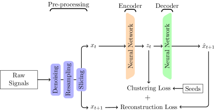
Figure 1: Diagram of the deep-seeded cluster algorithms based on k-means or c-means for signals. The definition of $q_{tk}$ and $\mu_{k}$ differentiate deep-seeded k-means from deep-seeded c-means.

II-A K-means and c-means

Clustering algorithms arrange data points by similarity. The well-established k-means algorithm splits data points into $K$ similarity groups called clusters.

Point $x_{t}$ is assigned to cluster $\mathcal{C}_{k}$, with $k\in\{1,\dots,K\}$ and $t\in\{0,\dots,T\}$, if $x_{t}$ is closer to the average characteristics of the points in cluster $\mathcal{C}_{k}$. The average of a cluster is called a centroid and denoted

$$\mu_{k}:=\frac{1}{|\mathcal{C}_{k}|}\sum_{t\in\mathcal{C}_{k}}x_{t}$$ (1)

If $x_{t}$ belongs to $\mathcal{C}_{k}$, assignment vector $s_{t}\in\{0,1\}^{K}$ satisfies

$$s_{tk}=\begin{cases}1,&\text{if }k=argmin_{l=1}^{K}||x_{t}-\mu_{k}||\\ 0,&\text{otherwise}\end{cases}$$ (2)

One can then obtain the optimum clusters by successively updating the assignment vectors and the centroids minimising the k-means’ loss function

$$L_{km}=\sum_{t=0}^{T}\sum_{k=1}^{K}s_{tk}||x_{t}-\mu_{k}||^{2}$$ (3)

C-means generalises k-means by assigning data points to fuzzy clusters instead of mutually exclusive clusters. According to Zhang et al. [46], observation $x_{t}$ belongs to cluster $k$ with degree

$$u_{tk}=\frac{exp\left(-\frac{2}{\gamma}\frac{||x_{t}-\mu_{k}||^{2}}{1+||x_{t}-\mu_{k}||^{2}}\right)}{\sum_{l=1}^{K}exp\left(-\frac{2}{\gamma}\frac{||x_{t}-\mu_{l}||^{2}}{1+||x_{t}-\mu_{l}||^{2}}\right)}$$ (4)

with $\gamma>0$. The higher is $u_{ik}$, the more $x_{t}$ belongs to cluster $\mathcal{C}_{k}$. Moreover, $\mu_{k}$ centroid of fuzzy cluster $\mathcal{C}_{k}$ is defined by

$$\mu_{k}=\frac{\sum_{t=0}^{T}d_{tk}u_{tk}x_{t}}{\sum_{s=0}^{T}d_{sk}u_{sk}}$$ (5)

where

$$d_{tk}=\frac{||x_{t}-\mu_{k}||+2}{(||x_{t}-\mu_{k}||+1)^{2}}$$ (6)

C-means’ estimation steps are the same as those of k-means. Successively updating the assignment vectors from eq. 4 and the centroids from eq. 5 and minimising the c-means’ loss

$$L_{cm}=\sum_{t=0}^{T}\sum_{k=1}^{K}u_{tk}||x_{t}-\mu_{k}||^{2}$$ (7)

K-means and c-means proved their utility in countless domains. Nonetheless, if the data points do not contain informative features, these methods fail to form meaningful clusters [47]. In our proposed method, we jointly estimate the c-means (and k-means for comparison) and an auto-encoder, to categorise the discovered embedded features from the original signal.

II-B Sequence-to-Sequence auto-encoder

An autoencoder is an artificial neural network (ANN) that learns an efficient latent space, typically in a lower dimensional space, that is validated and refined by regenerating the original input. First, a function $\varphi$, called an encoder, maps the observations $(x_{i})_{i=1}^{n}$ into a latent feature space. Second, the function $\psi$, called a decoder, maps back the latent vectors into the observation space. Latent features $z_{i}:=\varphi(x_{i})$ correctly encode observation $x_{i}$ if the decoded point $\hat{x}_{i}:=\psi(z_{i})$ is close enough to $x_{i}$, i.e. $||x_{i}-\hat{x}_{i}||<\epsilon$ for some $\epsilon>0$.

In the state-of-the-art, $\varphi$ and $\psi$ are ANNs. The optimal weights of $\varphi$ and $\psi$, respectively $w_{\varphi}$ and $w_{\psi}$, often minimise the reconstruction loss

$$L_{r}=\sum_{i=1}^{N}||x_{i}-\hat{x}_{i}||^{2}$$

In our case, we intend to extract features from the signal windows of size $\delta$, $(x_{t})_{t=0}^{T}$. In consequence, we use the sequence-to-sequence auto-encoder (S2S) [43] that is specifically designed for signal feature extraction.

Contrary to the standard auto-encoders, S2S’s decoder $\psi$ forecasts the next signal window [43]. In consequence, we say that the latent vector $z_{t}=\varphi(x_{t})$ correctly encodes observation $x_{t}$ if $\hat{x}_{t+1}=\psi(z_{t})$ is close enough to $x_{t+1}$, i.e. $||x_{t+1}-\hat{x}_{t+1}||<\epsilon$ for some $\epsilon$. Here, the optimal weights of $\varphi$ and $\psi$, respectively $w_{\varphi}$ and $w_{\psi}$, minimise the reconstruction loss

$$L_{r}=\sum_{t=0}^{T-\delta-1}||x_{t+1}-\hat{x}_{t+1}||^{2}$$ (8)

The optimal latent representation $z_{t}$ of data point $x_{t}$ is not unique. Indeed, if $\varphi$ and $\psi$ are optimal such that $L_{r}$ is minimal, then, for any bijection $f$, $f\circ\varphi$ and $\psi\circ f^{-1}$ are also optimal. Consequently, finding encoders and decoders minimising the reconstruction loss is insufficient. The latent representations need to be specific to clustering. Deep cluster algorithms jointly minimise reconstruction and clustering losses to obtain a latent representation that is suitable for the clustering at stake.

II-C Deep-Clustering

Signal windows of size $\delta$, $(x_{t})_{t=1}^{T}$, admit infinitely many latent representations. Nonetheless, deep-cluster algorithms bound the informative representations to form consistent clusters.

Several measures evaluate the consistency of clusters. We say that clusters are optimal if the sum of distances between their elements and centroids (loss 3 or 7) is minimal over the possible latent representations. Conversely, specific features to the k-means or c-means problem minimise loss 3 or 7.

However, $z_{tk}=\mu_{k}$, for all $t$ and $k$ is a trivial solution for minimising k-means’ and c-means’ loss. Informative features avoid this pitfall. In consequence, we say that clusters are consistent if their clustering loss (3 or 7) is minimal over the informative latent representations. Thus, the consistent features minimise the reconstruction loss 8 and clustering loss 3 or 7.

Equivalently, the feature vectors are outputs of the encoder $\varphi$ i.e $z_{tk}=\varphi(x_{t})$, and the predicted next signal windows are the output of the decoder i.e. $\hat{x}_{t+1}=\psi(z_{tk})$, the feature vectors are informative and specific when the consistent weights of $\varphi$ and $\psi$ minimise the total loss

$$L_{total}=L_{r}+L_{c}$$ (9)

with $L_{c}$ is k-means’ or c-means’ loss.

K-means’ loss 3 and c-means’ loss 7 depend on the assignments $s_{tk}$ or memberships $u_{tk}$, and the centroids $\mu_{k}$, which depend itself on $\varphi$. Each deep-cluster algorithm’s iteration has two steps [45]. First, gradient descent actualises the weights of $\psi$ and $\varphi$ to minimise $L_{total}$. Second, Equation 2 updates the assignment vectors for k-means, or Equation 4 updates the memberships vectors for c-means. Third, Equation 1 updates the centroids $\mu_{k}$ for k-means or Equation 5 for c-means. Deep cluster algorithms repeat these three steps until convergence.

Demonstrating deep cluster convergence is straightforward. First, each gradient descent’s iteration $i$ updates the encoder and decoder from $\varphi^{i}$ and $\psi^{i}$ to $\varphi^{i+1}$ and $\psi^{i+1}$ such that

$$L_{r}^{i+1}+\sum_{t=0}^{T}\sum_{k=1}^{K}q_{tk}^{i}||\varphi^{i+1}(x_{t}) -\mu_{k}^{i}||^{2}\leq L_{r}^{i}$$

$$+\sum_{t=0}^{T}\sum_{k=1}^{K}q_{tk}^{i}||\varphi^{i}(x_{t})-\mu_{k}^{i}||^{2}$$

where $q_{t}^{i}$ is k-means’ assignment or c-means’ membership vector of observation $t$ at iteration $i$. Second, k-means [48] or c-means [49] converge such that

$$\sum_{t=0}^{T}\sum_{k=1}^{K}q_{tk}^{i+1}||\varphi^{i+1}(x_{t})-\mu_{k}^{i+1}||^{2}\leq\sum_{t=0}^{T}\sum_{k=1}^{K}q_{tk}^{i}||\varphi^{i+1}(x_{t})-\mu_{k}^{i}||^{2}$$

In consequence, the deep cluster algorithm converges such that $L_{total}^{i+1}\leq L_{total}^{i}$.

To summarise, deep cluster algorithms form consistent clusters by extracting informative and specific features from observations. Nonetheless, the clusters’ contents remain unknown.

II-D Seeding

Though consistent, the clusters formed by the deep cluster algorithms have no label. If a deep cluster algorithm assigns the window of size $\delta$ of physiological signal $x_{t}$ to cluster $k$, no one can say what emotion the individual felt from $t$ to $t+\delta$. However, carefully initialising the algorithm can reveal what the clusters represent. This method is called seeding [37] [50].

We propose a simple seeding. If individuals assess that emotion $k^{*}$ was dominant from $T_{1}$ to $T_{2}$, physiological signal windows $(x_{t})_{t=T_{1}}^{T_{2}}$ are likely to have recorded this emotion’s physiological response. For k-means clustering, we initialise $s_{tk^{*}}=1,s_{tk}=0$ for all $t\in\{T_{1},\dots,T_{2}\}$ and $k\neq k^{*}$. However, we fix $s_{tk}=0$ for all $t\notin\{T_{1},\dots,T_{2}\}$ and $k\in\{1,\dots,K\}$. For c-means clustering, we initialise $u_{k^{*}1}=1,u_{tk}=0$ for all $t\in\{T_{1},\dots,T_{2}\}$ and $k\neq k^{*}$. Thereby, emotion $k^{*}$ defines the pseudo-label of cluster $k^{*}$. Contrariwise, observations outside $\{T_{1},\dots,T_{2}\}$ do not belong a priori more to one cluster than another. Thus, we initialise $u_{tk}=\frac{1}{K}$ for all $t\notin\{T_{1},\dots,T_{2}\}$ and $k\in\{1,\dots,K\}$. This operation is repeated for all the dominant emotions reported by the individuals.

Of course, emotion $k^{*}$ may have been more intense around $T_{1}$ than $T_{2}$, or arisen outside this period. However, each iteration of the algorithm adjusts $s_{tk^{*}}$ or $u_{tk^{*}}$ for all $t$ inside and outside $[T_{1},T_{2}]$.

Furthermore, the more emotion $k^{*}$ is manifest, the higher c-means’ cluster membership $u_{tk^{*}}$ is. Consequently, cluster membership $u_{tk^{*}}$ is interpreted as the intensity of emotion $k^{*}$ at time $t$.

II-E Pre-training

Recent parameter initialisation methods fasten network learning, and performance [51]. Pre-training is a type of initialisation method that brings the network’s parameters near their optimal value [52].

To improve emotion recognition performance, the S2S auto-encoder described in Subsection II-B can be trained to minimise the reconstruction loss 8 before performing deep seeded k-means and c-means.

The latent representation resulting from the reconstruction loss minimisation is informative but risks being non-specific. To bound the representation to be both informative and specific, the S2S auto-encoder is trained to minimise the total loss 9. The centroids are updated, but assignments or memberships initialised as described in Subsection II-D are not updated. We call this initialisation method constrained pre-training.

III Experimental evaluation

In this section, we test the algorithms introduced in Section II seeded k-means and seeded c-means, deep-seeded k-means and deep-seeded c-means to emotion recognition from EDA, BVP and skin temperature (ST) signals. The different architectures were implemented in an open-source Python code and compared using the WESAD benchmark data set. We also test if constrained pre-training improves the performance.

III-A Data set

The data set Wearable Stress and Affect Detection (WESAD) [12] has become a benchmark for testing emotion recognition methods. It includes data from a study to elicit three different affective states (neutral, stress, amusement) to 15 subjects with a mean age of 27.5 $\pm$ 2.4 years, where 12 subjects were male and the other three subjects were female. The subjects were also followed a guided meditation to de-excite them after the stress and amusement conditions.

During the experiment, the volunteers wear the wristband Empatica E4, measuring their EDA, BVP and ST. After each phase, the participants assess their valance and arousal levels through the Self-Assessment Manikin (SAM) questionnaire [53]. We slice the EDA, BVP and ST signals in overlapping windows of range. Then, the deep-seeded cluster for signals algorithm extract and cluster features from each window. The clusters are beforehand seeded with the answers to the SAM questionnaire. Comparing the pseudo-label assigned to the signal windows to experimental phase when they were recorded gives a measure of the accuracy of our method.

III-B Signal pre-processing

Feature extraction from raw EDA, BVP and ST signals is more efficient after pre-processing. In our proposed method we first apply a Savitzky-Golay filter to mitigate errors and remove outliers on the EDA and ST signals.

The EDA and ST signals were sampled at 4hz, while the BVP signal is sampled at 64hz, thus a zero-phase low-pass filter up-sampled the EDA and ST signals to the length of the BVP signal. Up-sampling the shorter signals instead of down-sampling the longest signal avoids information loss.

Thirdly, min-max-normalisation was applied to the three signals for speeding up the automatic feature extraction and improving the clustering [54].

Finally, the signals were sliced in overlapping windows of range $20$ and step $1$.

III-C Practical implementation

After testing different configurations, we opted for the architecture in Figure 1. The encoder and decoder formed by two gated recurrent units (GRU) layers efficiently reconstruct the EDA, BVP and ST signals while minimising the number of parameters. In addition, the three-neuron dense layer at the decoder’s end helps reconstruct the original signals without substantially increasing the overall network complexity. Moreover, the encoder and decoder’s recurrent layers are followed by normalisation layers. Standardising layers’ outputs, i.e. $(x-\mu)/\sigma$, reduces the training time [55] and improves clustering [54] of the latent vectors. Furthermore, the encoder extracts $30$ features. $\gamma$ is fixed to $1/2$ and the learning rate to $5\times 10^{-5}$.

Before training, the deep k-means’ and deep c-means’ auto-encoders are trained during a single epoch. The constrained pre-training lasts one or two epochs. The training follows pre-training with the total loss 9 for two epochs.

III-D Seeding

As described in Subsection II-D, we initialise the membership function with subjective data.

Table I shows the average arousal and valence scores measured through SAM questionnaires. The average valence and arousal are characteristic of stress, amusement and relaxation [42].

First, phase C aroused relaxation as it has the lowest arousal. Second, phase B aroused amusement as it has high arousal and valence. Third, phase D aroused stress as it has high arousal but low valence. In contrast, phase A corresponds to a neutral emotion.

Phase     Valence Arousal     Presumed emotion  A     6.7 2.5     Neutral B     7.5 3     Amusement C     6.5 2.3     Relaxation D     4.5 6.8     Stress

TABLE I: Average valence and arousal score, and presumed emotions for each phase

III-E Results

Contrary to k-means, c-means and deep c-means return degrees of cluster memberships. To measure the performance of this algorithm, we assign pseudo-label $\hat{y}_{t}$ to signal window $x_{t}$ if $\hat{y}_{t}$ is the cluster with the largest membership, i.e. $\hat{y}_{t}=argmax_{k=1}^{K}u_{tk}$. Then, the F1-score measures the accuracy of the pseudo labels against the WESAD stimuli. Comparing models with the F1-score is necessary because the durations of the stimuli are imbalanced. Table II displays the average F1-scores and overall accuracy across WESAD subjects.

Table II shows that c-means has higher average F1-scores for all the emotions but amusement than k-means. However, both k-means and c-means display high discrepancy between the benchmark dataset’s participants.

Both regard F1-score averages and standard deviation, deep cluster algorithms dominate k-means and c-means.

Nonetheless, the effect of constrained pre-training (CPT) is slight. CPT does not improve deep k-means for neutral emotion and stress recognition. Nonetheless, CPT deep k-means increases by 18% and 5% the recognition of amusement and relaxation while dividing the F1-score standard derivation by 3. Nonetheless, CPT for two epochs does not increase deep k-means performance.

Furthermore, CPT hinders deep c-means from recognising neutral emotion and stress. However, it increased by 34% and 14% amusement and relaxation recognition while dividing by 8 the F1 score standard deviation. Thus, CPT improves deep k-means and c-means amusement and relaxation recognition. Nonetheless, CPT for two epochs does not increase deep c-means performance.

Finally, CPT deep k-means and c-means have comparable overall accuracy. However, CPT deep k-means slightly better identifies stress, amusement and relaxation.

To conclude, deep k-means and c-means drastically improve emotion recognition compared to k-means and c-means. Moreover, CPT increases deep k-means and c-means amusement and relaxation recognition. Nonetheless, understanding why k-means and c-means-based algorithms remain to be explored.

    neutral stress amusement relaxation     accuracy random     30.52 (0) 23.49 (0) 16.58 (0) 25.61 (0)     25.00 (0)  k-means     49.22 (37) 79.52 (32) 39.02 (20) 54.64 (23)     56.60 (15) deep k-means     84.23 (9) 94.18 (3) 71.40 (16) 82.22 (17)     84.32 (7) CPT deep k-means     85.60 (5) 93.08 (3) 84.33 (8) 86.23 (6)     87.20 (4) 2-CPT deep k-means     86.72 (4) 92.69 (3) 83.49 (9) 87.00 (4)     87.73 (4)  c-means     77.05 (18) 82.64 (28) 26.38 (27) 64.97 (14)     69.45 (12) deep c-means     97.19 (3) 98.76 (1) 61.90 (37) 70.20 (40)     88.44 (10) CPT deep c-means     91.49 (3) 91.70 (3) 83.23 (5) 80.36 (5)     87.42 (3) 2-CPT deep c-means     91.32 (3) 92.18 (3) 83.49 (4) 81.71 (5)     87.86 (2)

TABLE II: F1-score in percentage (standard deviation), CPT stands for Constrained Pre-Training, 2-CPT indicates that CPT lasted 2 epochs (highest F1 scores printed in bold)

IV Conclusion

This article has introduced deep seeded k-means and c-means for physiological signals and a method to pre-train their auto-encoders. These algorithms automatically extract features from physiological signals to form consistent clusters. Moreover, seeding the clusters with subjective assessments reveals the emotion they contain. Thanks to identification, cluster memberships formed by c-means-based algorithms represent the intensity of emotions.

Benchmark tests reveal that deep seeded k-means and c-means recognise the four quadrants of the circumplex model of affect. Moreover, pre-training increases the distinction between positive and negative valence and reduces the discrepancy between benchmark’s individuals.

Nonetheless, a new auto-encoder architecture could improve the performance of deep c-means and deep k-means. Finally, future work could use the deep seeded k-means or c-means algorithm to reveal the effect of daily activities on mood.

V Acknoledgements

This work was supported by the European Union’s Horizon 2020 Research and Innovation Programme under the grant agreement No 945307 (eMOTIONAL Cities).

References

- [1] R. W. Picard, Affective computing. MIT press, 2000.
- [2] L. Shu, J. Xie, M. Yang, Z. Li, Z. Li, D. Liao, X. Xu, and X. Yang, “A review of emotion recognition using physiological signals,” Sensors, vol. 18, no. 7, p. 2074, 2018.
- [3] P. J. Bota, C. Wang, A. L. Fred, and H. P. Da Silva, “A review, current challenges, and future possibilities on emotion recognition using machine learning and physiological signals,” IEEE Access, vol. 7, pp. 140990–141020, 2019.
- [4] S. Gedam and S. Paul, “Automatic stress detection using wearable sensors and machine learning: A review,” in 2020 11th International Conference on Computing, Communication and Networking Technologies (ICCCNT), pp. 1–7, IEEE, 2020.
- [5] J. Zhang, Z. Yin, P. Chen, and S. Nichele, “Emotion recognition using multi-modal data and machine learning techniques: A tutorial and review,” Information Fusion, vol. 59, pp. 103–126, 2020.
- [6] M. A. Hasnul, N. A. A. Aziz, S. Alelyani, M. Mohana, and A. A. Aziz, “Electrocardiogram-based emotion recognition systems and their applications in healthcare—a review,” Sensors, vol. 21, no. 15, p. 5015, 2021.
- [7] Y. Zhang, J. Wang, Y. Chen, H. Yu, and T. Qin, “Adaptive memory networks with self-supervised learning for unsupervised anomaly detection,” IEEE Transactions on Knowledge and Data Engineering, 2022.
- [8] S. Li and W. Deng, “Deep facial expression recognition: A survey,” IEEE transactions on affective computing, vol. 13, no. 3, pp. 1195–1215, 2020.
- [9] P. Shen, Z. Changjun, and X. Chen, “Automatic speech emotion recognition using support vector machine,” in Proceedings of 2011 international conference on electronic & mechanical engineering and information technology, vol. 2, pp. 621–625, IEEE, 2011.
- [10] A. Anusha, P. Sukumaran, V. Sarveswaran, A. Shyam, T. J. Akl, S. Preejith, M. Sivaprakasam, et al., “Electrodermal activity based pre-surgery stress detection using a wrist wearable,” IEEE journal of biomedical and health informatics, vol. 24, no. 1, pp. 92–100, 2019.
- [11] T. Song, W. Zheng, P. Song, and Z. Cui, “Eeg emotion recognition using dynamical graph convolutional neural networks,” IEEE Transactions on Affective Computing, vol. 11, no. 3, pp. 532–541, 2018.
- [12] P. Schmidt, A. Reiss, R. Duerichen, C. Marberger, and K. Van Laerhoven, “Introducing wesad, a multimodal dataset for wearable stress and affect detection,” in Proceedings of the 20th ACM international conference on multimodal interaction, pp. 400–408, 2018.
- [13] R. W. Picard, E. Vyzas, and J. Healey, “Toward machine emotional intelligence: Analysis of affective physiological state,” IEEE transactions on pattern analysis and machine intelligence, vol. 23, no. 10, pp. 1175–1191, 2001.
- [14] S. Katada, S. Okada, Y. Hirano, and K. Komatani, “Is she truly enjoying the conversation? analysis of physiological signals toward adaptive dialogue systems,” in Proceedings of the 2020 International Conference on Multimodal Interaction, pp. 315–323, 2020.
- [15] A. Jimenez-Molina, C. Retamal, and H. Lira, “Using psychophysiological sensors to assess mental workload during web browsing,” Sensors, vol. 18, no. 2, p. 458, 2018.
- [16] E. Diener, R. E. Lucas, and C. N. Scollon, “Beyond the hedonic treadmill: Revising the adaptation theory of well-being,” in The science of well-being, pp. 103–118, Springer, 2009.
- [17] C. R. Reynolds and L. A. Suzuki, “Bias in psychological assessment: An empirical review and recommendations,” Handbook of Psychology, Second Edition, vol. 10, 2012.
- [18] S. J. Raudys, A. K. Jain, et al., “Small sample size effects in statistical pattern recognition: Recommendations for practitioners,” IEEE Transactions on pattern analysis and machine intelligence, vol. 13, no. 3, pp. 252–264, 1991.
- [19] X. Zhu, C. Vondrick, C. C. Fowlkes, and D. Ramanan, “Do we need more training data?,” International Journal of Computer Vision, vol. 119, no. 1, pp. 76–92, 2016.
- [20] H. P. Martinez, Y. Bengio, and G. N. Yannakakis, “Learning deep physiological models of affect,” IEEE Computational intelligence magazine, vol. 8, no. 2, pp. 20–33, 2013.
- [21] S. A. H. Aqajari, E. K. Naeini, M. A. Mehrabadi, S. Labbaf, N. Dutt, and A. M. Rahmani, “pyeda: An open-source python toolkit for pre-processing and feature extraction of electrodermal activity,” Procedia Computer Science, vol. 184, pp. 99–106, 2021.
- [22] M. Neumann and N. T. Vu, “Improving speech emotion recognition with unsupervised representation learning on unlabeled speech,” in ICASSP 2019-2019 IEEE International Conference on Acoustics, Speech and Signal Processing (ICASSP), pp. 7390–7394, IEEE, 2019.
- [23] J. O. Huelle, B. Sack, K. Broer, I. Komlewa, and S. Anders, “Unsupervised learning of facial emotion decoding skills,” Frontiers in human neuroscience, vol. 8, p. 77, 2014.
- [24] Z. Lian, J. Tao, B. Liu, and J. Huang, “Unsupervised representation learning with future observation prediction for speech emotion recognition,” arXiv preprint arXiv:1910.13806, 2019.
- [25] S. E. Eskimez, Z. Duan, and W. Heinzelman, “Unsupervised learning approach to feature analysis for automatic speech emotion recognition,” in 2018 IEEE International Conference on Acoustics, Speech and Signal Processing (ICASSP), pp. 5099–5103, IEEE, 2018.
- [26] J. Tervonen, S. Puttonen, M. J. Sillanpää, L. Hopsu, Z. Homorodi, J. Keränen, J. Pajukanta, A. Tolonen, A. Lämsä, and J. Mäntyjärvi, “Personalized mental stress detection with self-organizing map: From laboratory to the field,” Computers in Biology and Medicine, vol. 124, p. 103935, 2020.
- [27] M. Kang, S. Shin, J. Jung, and Y. Kim, “Stress classification using k-means clustering and heart rate variability from electrocardiogram,” International Journal of Biology and Biomedical Engineering, vol. 14, pp. 251–254, 01 2021.
- [28] X. Zhuang, V. Rozgić, and M. Crystal, “Compact unsupervised eeg response representation for emotion recognition,” in IEEE-EMBS international conference on Biomedical and Health Informatics (BHI), pp. 736–739, IEEE, 2014.
- [29] E. Vildjiounaite, J. Kallio, J. Mäntyjärvi, V. Kyllönen, M. Lindholm, and G. Gimel’farb, “Unsupervised stress detection algorithm and experiments with real life data,” in EPIA Conference on Artificial Intelligence, pp. 95–107, Springer, 2017.
- [30] D. Huysmans, E. Smets, W. De Raedt, C. Van Hoof, K. Bogaerts, I. Van Diest, and D. Helic, “Unsupervised learning for mental stress detection-exploration of self-organizing maps,” Proc. of Biosignals 2018, vol. 4, pp. 26–35, 2018.
- [31] C. Maaoui and A. Pruski, “Unsupervised stress detection from remote physiological signal,” in 2018 IEEE International Conference on Industrial Technology (ICIT), pp. 1538–1543, IEEE, 2018.
- [32] Y. Wu, M. Daoudi, A. Amad, L. Sparrow, and F. D’Hondt, “Unsupervised learning method for exploring students’ mental stress in medical simulation training,” in Companion Publication of the 2020 International Conference on Multimodal Interaction, pp. 165–170, 2020.
- [33] K. Lai, S. N. Yanushkevich, and V. P. Shmerko, “Intelligent stress monitoring assistant for first responders,” IEEE Access, vol. 9, pp. 25314–25329, 2021.
- [34] S. Deldari, D. V. Smith, A. Sadri, and F. Salim, “Espresso: Entropy and shape aware time-series segmentation for processing heterogeneous sensor data,” Proceedings of the ACM on Interactive, Mobile, Wearable and Ubiquitous Technologies, vol. 4, no. 3, pp. 1–24, 2020.
- [35] A. Kumar, K. Sharma, and A. Sharma, “Genetically optimized fuzzy c-means data clustering of iomt-based biomarkers for fast affective state recognition in intelligent edge analytics,” Applied Soft Computing, vol. 109, p. 107525, 2021.
- [36] Z. Liang, S. Oba, and S. Ishii, “An unsupervised eeg decoding system for human emotion recognition,” Neural Networks, vol. 116, pp. 257–268, 2019.
- [37] S. Basu, A. Banerjee, and R. Mooney, “Semi-supervised clustering by seeding,” in In Proceedings of 19th International Conference on Machine Learning (ICML-2002, Citeseer, 2002.
- [38] S. Jerritta, M. Murugappan, R. Nagarajan, and K. Wan, “Physiological signals based human emotion recognition: a review,” in 2011 IEEE 7th international colloquium on signal processing and its applications, pp. 410–415, IEEE, 2011.
- [39] A. Saxena, A. Khanna, and D. Gupta, “Emotion recognition and detection methods: A comprehensive survey,” Journal of Artificial Intelligence and Systems, vol. 2, no. 1, pp. 53–79, 2020.
- [40] B. Yang, X. Han, and J. Tang, “Three class emotions recognition based on deep learning using staked autoencoder,” in 2017 10th International Congress on Image and Signal Processing, BioMedical Engineering and Informatics (CISP-BMEI), pp. 1–5, IEEE, 2017.
- [41] Z. Yin, Y. Wang, W. Zhang, L. Liu, J. Zhang, F. Han, and W. Jin, “Physiological feature based emotion recognition via an ensemble deep autoencoder with parsimonious structure,” IFAC-PapersOnLine, vol. 50, no. 1, pp. 6940–6945, 2017.
- [42] J. A. Russell, “A circumplex model of affect.,” Journal of personality and social psychology, vol. 39, no. 6, p. 1161, 1980.
- [43] I. Sutskever, O. Vinyals, and Q. V. Le, “Sequence to sequence learning with neural networks,” Advances in neural information processing systems, vol. 27, 2014.
- [44] J. Yang, D. Parikh, and D. Batra, “Joint unsupervised learning of deep representations and image clusters,” in Proceedings of the IEEE conference on computer vision and pattern recognition, pp. 5147–5156, 2016.
- [45] B. Yang, X. Fu, N. D. Sidiropoulos, and M. Hong, “Towards k-means-friendly spaces: Simultaneous deep learning and clustering,” in international conference on machine learning, pp. 3861–3870, PMLR, 2017.
- [46] R. Zhang, X. Li, H. Zhang, and F. Nie, “Deep fuzzy k-means with adaptive loss and entropy regularization,” IEEE Transactions on Fuzzy Systems, vol. 28, no. 11, pp. 2814–2824, 2019.
- [47] M. Capó, A. Pérez, and J. A. Lozano, “A cheap feature selection approach for the k-means algorithm,” IEEE transactions on neural networks and learning systems, vol. 32, no. 5, pp. 2195–2208, 2020.
- [48] L. Bottou and Y. Bengio, “Convergence properties of the k-means algorithms,” Advances in neural information processing systems, vol. 7, 1994.
- [49] R. J. Hathaway and J. C. Bezdek, “Recent convergence results for the fuzzy c-means clustering algorithms,” Journal of Classification, vol. 5, no. 2, pp. 237–247, 1988.
- [50] E. Bair, “Semi-supervised clustering methods,” Wiley Interdisciplinary Reviews: Computational Statistics, vol. 5, no. 5, pp. 349–361, 2013.
- [51] C. A. de Sousa, “An overview on weight initialization methods for feedforward neural networks,” in 2016 International Joint Conference on Neural Networks (IJCNN), pp. 52–59, IEEE, 2016.
- [52] M. V. Narkhede, P. P. Bartakke, and M. S. Sutaone, “A review on weight initialization strategies for neural networks,” Artificial intelligence review, vol. 55, no. 1, pp. 291–322, 2022.
- [53] S. Koelstra, C. Muhl, M. Soleymani, J.-S. Lee, A. Yazdani, T. Ebrahimi, T. Pun, A. Nijholt, and I. Patras, “Deap: A database for emotion analysis; using physiological signals,” IEEE transactions on affective computing, vol. 3, no. 1, pp. 18–31, 2011.
- [54] K. A. Doherty, R. Adams, and N. Davey, “Unsupervised learning with normalised data and non-euclidean norms,” Applied Soft Computing, vol. 7, no. 1, pp. 203–210, 2007.
- [55] J. L. Ba, J. R. Kiros, and G. E. Hinton, “Layer normalization,” arXiv preprint arXiv:1607.06450, 2016.