Closed-form approximations of moments and densities of continuous–time Markov models

Abstract

This paper develops power series expansions of a general class of moment functions, including transition densities and option prices, of continuous-time Markov processes, including jump–diffusions. The proposed expansions extend the ones in Kristensen and Mele (2011) to cover general Markov processes. We demonstrate that the class of expansions nests the transition density and option price expansions developed in Yang et al. (2019) and Wan and Yang (2021) as special cases, thereby connecting seemingly different ideas in a unified framework. We show how the general expansion can be implemented for fully general jump–diffusion models. We provide a new theory for the validity of the expansions which shows that series expansions are not guaranteed to converge as more terms are added in general. Thus, these methods should be used with caution. At the same time, the numerical studies in this paper demonstrate good performance of the proposed implementation in practice when a small number of terms are included.

JEL Classification: C13; C32; C63; G12; G13.

Keywords: Continuous-time models, jump-diffusion, transition density, stochastic volatility, closed-form approximations, maximum-likelihood estimation, option pricing.

1 Introduction

Continuous-time jump-diffusion processes are used in economics and finance to model the dynamics of state variables (see, e.g., Björk, 2009). They lead to a simple and elegant analysis of problems such as the pricing of financial assets, portfolio management and other dynamic phenomena. This comes at a big computational cost though: Many relevant characteristics, such as moments and densities, of such processes cannot be expressed in closed-form except in a few special cases. This hampers their practical use and implementation. This has led researchers to develop numerical methods for the computation of these. Broadly speaking, these methods fall in three categories: Finite–difference methods (Ames, 1992), simulation–based methods (see, e.g., Elerian et al., 2001; Brandt and Santa-Clara, 2002; Durham and Gallant, 2002; Beskos et al., 2009; Kristensen and Shin, 2012; Sermaidis et al., 2013) and series expansions (see, e.g., Aït-Sahalia, 2002; Bakshi et al., 2006; Yu, 2007; Aït-Sahalia, 2008; Filipović et al., 2013; Li, 2013). This paper focuses on the latter category.

Most existing expansions proposed in the literature are application specific: Depending on the particular features of the chosen moment and model of the underlying stochastic process, different methods have been developed. One exception is Kristensen and Mele (2011) who developed power series expansions that covered a general class of moment functions and the transition density of multivariate diffusion processes. Their focus was on applications to option pricing but the class of expansions applies more generally. The current paper makes four contributions:

First, we demonstrate that the class of series expansions of Kristensen and Mele (2011) are easily extended to cover fully general continuous–time Markov models, including any jump–diffusion process. Thus, the proposal of Kristensen and Mele (2011) can in principle be applied to any moment of any Markov process. As part of this extension, we present a novel derivation and representation of the series expansion of Kristensen and Mele (2011). This new representation highlights important features of the original expansion that was perhaps not obvious from the analysis of Kristensen and Mele (2011).

Second, we revisit the recent work of Yang et al. (2019) and Wan and Yang (2021) and demonstrate that in fact their proposed expansions of transition densities and option prices are special cases of Kristensen and Mele (2011). Thus, at a theoretical level the expansions in Yang et al. (2019) and Wan and Yang (2021) are not new. At the same time, it should be emphasized that Yang et al. (2019) and Wan and Yang (2021) make important contributions in terms of the practical implementation of the proposal in Kristensen and Mele (2011). They develop numerical algorithms that allow for fast implementation of the general method of Kristensen and Mele (2011) when applied to transition densities and option prices of diffusion processes and a limited set of jump–diffusion processes. As such, the current paper should hopefully clarify the relationship between these three existing papers and their relative contributions to the literature.

Third, we propose a novel numerical implementation of our series expansions when applied to general jump–diffusion models. The algorithms of Kristensen and Mele (2011) and Yang et al. (2019) are restricted to pure diffusions while the extension found in Wan and Yang (2021) requires the jump component to be fully independent of the diffusive component. That is, the jump intensity and the jump sizes are not allowed to be state–dependent. Our numerical implementation allows for both to be state–dependent. We demonstrate through a series of numerical studies that our numerical method works well in practice.

Fourth, we provide a novel theory for the validity of power series expansions of moment functions of continuous–time Markov processes used here and elsewhere in the literature, including all above references to papers employing series–based approximations. Most existing theoretical results for these expansions only show that a given moment expansion converges as the time interval over which the conditional moment is defined shrinks to zero. As such existing results provide no guarantees that the approximation error will get smaller as more terms are added to expansion; in fact, nothing rules out that the approximation error may actually explode as more terms are added. For the power series expansion to be reliable, it is desirable with conditions under which the expansions converge not only over shrinking time intervals but also over a fixed time interval. We here provide guarantees for the approximations to be numerically stable as the order of the approximation grows. Our theoretical results rely on semi–group theory as also used by, e.g., Hansen and Scheinkman (1995) to analyze the properties of continuous–time Markov processes.

Our theoretical results demonstrate that power series expansions of Markov moments may very well not converge: The chosen moment and model has to satisfy certain regularity conditions for this to hold. In particular, we demonstrate that the expansions of transition densities and option prices proposed by Kristensen and Mele (2011), Yang et al. (2019) and Wan and Yang (2021) do not converge. That is, these methods are bound to fail as the number of series terms grows. As such, the expansions proposed in these papers and the extension to general jump–diffusions developed here should be used with care. In particular, researchers may not wish to add more than, say, 4–5 terms to the expansion in order to avoid the numerical error to blow up.

The remains of the paper are organized as follows. Section 2 presents series expansions of a broad class of moments and densities of basically any continuous–time Markov process. In section 3, we propose a numerical implementation of the general method when applied to general jump–diffusion models. Section 4 analyzes the theoretical properties of the power series expansion over both shrinking and fixed time distances. Section 5 examines the numerical performance of our numerical algorithm. Section 6 concludes. Appendix C gathers all proofs.

2 Moment expansions of Markov processes

We first provide a motivating example of a jump–diffusion model and some of the moments researchers often are interested in computing. We then proceed to consider more general framework and develop a general moment expansion method in this setting.

2.1 Motivating example

Consider a $d$-dimensional process, $x_{t}\in\mathcal{X\subseteq}\mathbb{R}^{d}$ that solves the following stochastic differential equation (SDE):

$$dx_{t}=\mu\left(x_{t}\right)dt+\sigma\left(x_{t}\right)dW_{t}+J_{t}dN_{t},$$ (2.1)

where $\mu\left(x\right)$ and $\sigma\left(x\right)$ are the so-called drift and diffusion functions, respectively, $W_{t}$ is a $d$-dimensional standard Brownian motion, $N_{t}$ is a Poisson process with jump intensity $\lambda\left(x_{t}\right)$, and $J_{t}$ captures the jump-sizes and has conditional density $\nu\left(\cdot|x_{t}\right)$. The precise form of $\mu\left(x\right)$, $\sigma\left(x\right)$, $\lambda\left(x\right)$ and $\nu\left(\cdot|x\right)$ are chosen by the researcher according to the dynamic problem that is being considered and so are known to us. To keep notation simple, we restrict ourselves to the time–homogenous case meaning that none of the functions entering the model depend on $t$; the extension to the time–inhomogenous case can be found in Appendix B.

We are interested in computing conditional moments on the form

$$u_{t}\left(x\right)=E_{t}f\left(x\right)$$ (2.2)

where

$$\left(t,f\right)\mapsto E_{t}f\left(x\right)\equiv\mathbb{E}\left[\left.\exp\left(-\int\nolimits_{0}^{t}r\left(x_{s}\right)ds\right)f\left(x_{t}\right)\right|x_{0}=x\right]$$ (2.3)

is a conditional moment operator. This family of operators, indexed by the time variable $t\geq 0$, constitutes a so–called semi–group of linear operators; for an overview of the general theory of semi–groups with applications to Markov processes we refer to Ethier and Kurtz (1986); for applications of semi–group theory in econometrics and finance, see Aït-Sahalia et al. (2010).

The functions $r\left(x\right)$ and $f\left(x\right)$ entering (2.2)–(2.3) are chosen by the researcher according to the problem of interest. For example, with $r\left(x\right)=0$ and $f\left(x\right)=\delta\left(y-x\right)$ for some fixed $y\in\mathcal{X}$, where $\delta\left(x\right)$ is Dirac’s Delta function, $u_{t}\left(x\right)=p_{t}\left(y|x\right)$, where $p_{t}$ is the transition density of $x_{t}$,

$$\Pr\left(x_{t}\in\mathcal{A}|x_{0}=x\right)=\int_{\mathcal{A}}p_{t}\left(y|x\right)dy,\text{ \ \ }\mathcal{A}\subseteq\mathcal{X}.$$

If instead we choose $r_{t}\left(x\right)=r>0$ and $f\left(x\right)=\left(\exp\left(x_{1}\right)-K\right)^{+}$ then $u_{t}\left(x\right)$ becomes the price of a European call option with time to maturity $t$ when the state variables $x_{t}$ satisfy (2.1) under the risk–neutral measure with the first component, $x_{1,t}$, being the log-price of the underlying asset and the short-term interest rate equals the constant $r$. When $r\left(x\right)=x_{2}$, $u_{t}\left(x\right)$ is the price of the same option but now allowing for a stochastic short–term interest rate, which is the second component of $x_{t}$.

In most cases, an analytic expression of (2.2) is not available and $u_{t}\left(x\right)$ has to be computed using numerical approximations. To motivate our proposed approximation of $u_{t}\left(x\right)$, observe that an equivalent representation of it is the solution to a partial integro-differential equation (PIDE). An important component of this PIDE is the so–called (infinitesimal) generator $A$ of $x_{t}$ which fully characterizes the dynamics. The generator is given by, for any sufficiently regular function $f\left(x\right)$,

$$Af\left(x\right)=A_{D}f\left(x\right)+A_{J}f\left(x\right),$$ (2.4)

where, with $\sigma^{2}\left(x\right):=\sigma\left(x\right)\sigma\left(x\right)^{\top}\in\mathbb{R}^{d\times d}$,

$$A_{D}f\left(x\right)=\sum_{i=1}^{d}\mu_{i}\left(x\right)\partial_{x_{i}}f\left(x\right)+\frac{1}{2}\sum_{i,j=1}^{d}\sigma_{ij,t}^{2}\left(x\right)\partial_{x_{i},x_{j}}^{2}f\left(x\right)$$ (2.5)

and

$$A_{J}f\left(x\right)=\lambda\left(x\right)\int_{\mathbb{R}^{d}}\left[f\left(x+c\right)-f\left(x\right)\right]\nu\left(c|x\right)dc$$ (2.6)

are the generators of the diffusive and jump component of $x_{t}$, respectively. Here, $\partial_{x_{i}}f\left(x\right)=\partial f\left(x\right)/\left(\partial x_{i}\right)$, $\partial_{x_{i},x_{j}}^{2}f\left(x\right)=\partial^{2}f\left(x\right)/\left(\partial x_{i}\partial x_{j}\right)$ and similar for other partial derivatives.

It can then be shown, c.f. Section 4, that $u_{t}\left(x\right)$ solves the following PIDE:

$$\partial_{t}u_{t}\left(x\right)=\left[A-r\left(x\right)\right]u_{t}\left(x\right),\text{ \ \ }t\geq 0,x\in\mathcal{X},$$ (2.7)

with initial condition $u_{0}\left(x\right)=f\left(x\right)$ for all $x\in\mathcal{X}$. In the case of pure diffusions ($A_{J}=0$), the reader may recognize (2.2) as the celebrated Feynman–Kac representation of the solution to (2.7) which also holds for the general case of jump–diffusions. The solution to this PIDE can be represented in the following abstract manner: $u_{t}\left(x\right)=e^{\left(A-r\right)t}f\left(x\right)$, where $e^{\left(A-r\right)t}$ is the exponential of the operator $A-r$ in the sense that

$$\frac{\partial e^{\left(A-r\right)t}}{\partial t}=\left(A-r\right)e^{\left(A-r\right)t}.$$ (2.8)

We are now interested in obtaining an approximation of $u_{t}\left(x\right)$ based on a series expansion w.r.t. time $t$. A simple version of this would be a Taylor series expansion around $t=0$ on the form

$$\tilde{u}_{t}\left(x\right)\equiv\sum\limits_{m=0}^{M}\frac{t^{m}}{m!}\left.\partial_{t}^{m}u_{t}\left(x\right)\right|_{t=0}=\sum\limits_{m=0}^{M}\frac{t^{m}}{m!}\left(A-r\right)^{m}f\left(x\right),$$ (2.9)

for some $M\geq 1$, where the second equality uses (2.8). This type of moment approximations have found widespread use in the literature; see, e.g., (see, e.g., Aït-Sahalia, 2002; Bakshi et al., 2006; Yu, 2007; Aït-Sahalia, 2008; Filipović et al., 2013; Li, 2013). However, this expansion is not valid (well-defined) when, for example, $f\left(x\right)$ is a non–smooth function since the domain of the operator $A_{D}$ is restricted to smooth functions, c.f. (2.5). The transition density and option pricing examples provided above fall in this category. We will now present a generalized version of above expansion that circumvents this issue; this is done for fully general semi–groups/Markov processes.

2.2 General framework

We take as given some semi–group $\left(t,f\right)\mapsto E_{t}f\left(x\right)$ of interest. It could, for example, be on the form (2.3) for some continuous–time Markov process $x_{t}$, not necessarily a jump–diffusion process. But we do not restrict ourselves to this case.

Suppose that $E_{t}f\left(x\right)$ is not available on closed form for a given choice of $f$; we here show how this can be approximated through a Taylor series expansion of $E_{t}f\left(x\right)$ w.r.t. $t$ when either $f$ is sufficiently regular, where the notion of ”regular” will be made clear below, or it can be expressed as the limit of a regular function. The proposal is a generalisation of the one of Kristensen and Mele (2011), but the derivation will be carried out using semi–group theory which simplifies the derivations substantially compared to Kristensen and Mele (2011) and provides new insights into the expansion.

Let $\mathcal{D}\left(E\right)$ denote the domain of $E$ and let $B$ be the infinitesimal operator of the semi–group defined as

$$Bf\left(x\right)=\lim_{t\rightarrow 0^{+}}\frac{E_{t}f\left(x\right)-f\left(x\right)}{t},$$

and let $\mathcal{D}\left(B\right)$ denote the domain of $B$; that is, the set of functions $f\in\mathcal{D}\left(E\right)$ for which the above limit exists. In the motivating jump–diffusion example, $B=A-r$. For any $f\in\mathcal{D}\left(E\right)$, we write

$$E_{t}f\left(x\right)=e^{Bt}f\left(x\right),$$ (2.10)

where as before this should be interpreted as

$$\partial_{t}E_{t}f\left(x\right)=BE_{t}f\left(x\right),\text{ \ \ }t>0.$$ (2.11)

If the chosen $f$ satisfies $f\in\mathcal{D}\left(B^{M}\right)$, (2.11) also holds at $t=0$ and so the following Taylor series expansion of $E_{t}f\left(x\right)$ w.r.t. $t$ around $t=0$ is valid,

$$\hat{E}_{t}f\left(x\right)\equiv\sum\limits_{m=0}^{M}\frac{t^{m}}{m!}\left.\partial_{t}^{m}E_{t}f\left(x\right)\right|_{t=0^{+}}=\sum\limits_{m=0}^{M}\frac{t^{m}}{m!}B^{m}f\left(x\right),$$ (2.12)

where under weak conditions $\tilde{E}_{t}f\left(x\right)=E_{t}f\left(x\right)+O\left(t^{M}\right)$. This is a generalised version of (2.9).

We are now interested in generalising this series expansion to also work when $f\notin\mathcal{D}\left(B^{M}\right)$. An important ingredient of this is to first identify/construct a smoothed version of $f\left(x\right)$, denoted $u_{0,s}\left(x\right)$, $s\geq 0$ and $x\in\mathcal{X}$, which we require to satisfy the following two conditions:

A.0

(i) $\lim_{s\rightarrow 0^{+}}u_{0,s}\left(x\right)=f\left(x\right)$ and (ii) $u_{0,s}\in\mathcal{D}\left(\left(\partial_{s}\right)^{M_{1}}\right)\cap\mathcal{D}\left(B^{M_{2}}\right)$ for some $s\geq 0$ and $M_{1},M_{2}\geq 1$.

The function $u_{0,s}\left(x\right)$ is chosen by the researcher and needs to be available on closed form for the subsequent approximation to be operational. The choice of $u_{0,s}\left(x\right)$ is application specific in the sense that Assumption A.0 has to be satisfied: Part (i) requires $u_{0,s}\left(x\right)$ to converge towards the irregular function of interest $f\left(x\right)\notin\mathcal{D}\left(B\right)$ as $s\rightarrow 0^{+}$. Part (ii) says that, for some $s>0$, $u_{0,s}\left(x\right)$ is sufficiently regular in the sense that it is $M$ times continuously differentiable in $s$ and each of these derivatives belongs to $\mathcal{D}\left(B^{M}\right)$.

Assumption A.0 allows for a broad range of smoothers. One choice of $u_{0,s}\left(x\right)$ which under great generality will satisfy A.0 is $u_{0,s}\left(x\right)=E_{0,s}f\left(x\right)$ where $E_{0}$ is another semi–group chosen such that $u_{0,s}\left(x\right)$ is available on closed form. This choice clearly satisfies part (i) and if $E_{0}$ has similar properties as the one of interest, $E$, so that their respective generators have shared domain, then part (ii) will also hold. A simple choice of $E_{0}$, as proposed by Kristensen and Mele (2011), is $E_{0,s}f\left(x\right)=E\left[f\left(x_{0,s}\right)|x_{0}=x\right],$where $x_{0,s}$ is another stochastic process specified by the researcher. The process $x_{0,t}$ could, for example, be chosen as a random walk type stochastic process with transition density $p_{0,s}\left(y|x\right)=K\left(\left(y-x\right)/\sqrt{s}\right)/\sqrt{s}$, for some kernel density $K:\mathbb{R}^{d}\mapsto\mathbb{R}^{d}$, in which case

$$u_{0,s}\left(x\right)=\frac{1}{\sqrt{s}}\int_{\mathbb{R}^{d}}f\left(y\right)K\left(\frac{y-x}{\sqrt{s}}\right)dy.$$ (2.13)

This choice satisfies (i) and if $K$ is $M_{1}$ times differentiable then $u_{0,s}\left(x\right)$ has the same property. The final requirement, $u_{0,s}\in\mathcal{D}\left(B^{M_{2}}\right)$, has to be checked on a case by case basis.

Under A.0, the following identity holds:

$$f\left(x\right)=u_{0,0}\left(x\right)=e^{\left(-\partial_{s}\right)s}u_{0,s}\left(x\right),$$

where the second equality simply states that $u_{0,0}\left(x\right)=u_{0,s}\left(x\right)+\int_{0}^{s}\left(-\partial_{\tau}\right)u_{0,\tau}\left(x\right)d\tau$. Substituting this into (2.10) yields

$$E_{t}f\left(x\right)=e^{Bt}e^{\left(-\partial_{s}\right)s}u_{0,s}\left(x\right)=e^{\left(-\partial_{s}\right)s}e^{Bt}u_{0,s}\left(x\right),$$ (2.14)

where the last equality uses the following fundamental result: If two infinitesimal operators, say, $B_{1}$ and $B_{2}$, commute in the sense that $B_{1}B_{2}f=B_{2}B_{1}f$ then $e^{B_{1}s}e^{B_{2}t}f=e^{B_{1}s+B_{2}t}f=e^{B_{2}t}e^{B_{1}s}f$. This applies to the case of $B$ and $\partial_{s}$, $\partial_{s}B=B\partial_{s}$, since $B$ acts on $x$ while $\partial_{s}$ acts on $s$.

Finally, carry out a Taylor series expansion w.r.t. $\left(s,t\right)$ to obtain

$$\hat{E}_{t}f\left(x\right)=\sum\limits_{m_{1}=0}^{M_{1}}\sum\limits_{m_{2}=0}^{M_{2}}\frac{\left(-s\right)^{m_{1}}t^{m_{2}}}{m_{1}!m_{2}!}B^{m_{2}}\partial_{s}^{m_{1}}u_{0,s}\left(x\right),$$ (2.15)

where the order of $\partial_{s}$ and $B$ can be exchanged since $\partial_{s}^{m_{1}}B^{m_{2}}u_{0,s}\left(x\right)=B^{m_{2}}\partial_{s}^{m_{1}}u_{0,s}\left(x\right)$. The resulting approximation error is of order $O\left(s^{M_{1}}\right)+O\left(t^{M_{2}}\right)$. In particular, the above expansion will generally be more precise as $s$ gets smaller. Thus, we ideally want to choose $s$ as small as possible to reduce the approximation error. However, for the chosen value of $s\geq 0$ A.0(ii) has to be satisfied. This rules out, for example, $s=0$ when $f$ is irregular since $u_{0,0}\left(x\right)=f\left(x\right)$.

However, if the approximation error is not a major concern (which is, for example, the case if the order of approximation can be chosen sufficiently large) then one can choose $s=t$ in which case $E_{t}f\left(x\right)=e^{\left(B-\partial_{t}\right)t}u_{0,t}\left(x\right)$ and the following special case of (2.15) can be employed,

$$\hat{E}_{t}f\left(x\right)=\sum\limits_{m=0}^{M}\frac{t^{m}}{m!}\left(B-\partial_{t}\right)^{m}u_{0,t}\left(x\right).$$ (2.16)

We show in Appendix A that (2.16) is a generalized version of the proposal of Kristensen and Mele (2011) which in turn contains as special cases the expansions of Yang et al. (2019) and Wan and Yang (2021).

3 Implementation of expansion for jump-diffusion models

This section provides details regarding the practical implementation of the proposed approximation in the jump–diffusion case. We here focus on the special case of $r\left(x\right)=0$ and $s=t$, in which case $u_{t}\left(x\right)=E_{t}f\left(x\right)=\mathbb{E}\left[f\left(x_{t}\right)|x_{0}=x\right]$ and

$$\hat{u}_{t}\left(x\right)=\sum\limits_{m=0}^{M}\frac{t^{m}}{m!}\left(A-\partial_{t}\right)^{m}u_{0,t}\left(x\right).$$ (3.1)

This is done to avoid overly complicated notation. Most of the ideas and arguments extend to the general case.

3.1 Choice of smoothing function for irregular moments

Following Kristensen and Mele (2011), a simple choice of $u_{0,s}\left(x\right)$ that satisfies A.1 is $u_{0,s}\left(x\right)=E_{0,s}f\left(x\right)=\mathbb{E}\left[f\left(x_{0,s}\right)|x_{0,0}=x\right]$ where $x_{0,s}$ is chosen as the solution to an auxiliary jump–diffusion model,

$$dx_{0,t}=\mu_{0}\left(x_{0,t}\right)dt+\sigma_{0}\left(x_{0,t}\right)dW_{t}+J_{0,t}dN_{0,t},$$ (3.2)

where $N_{0,t}$ is a Poisson process with jump intensity $\lambda_{0}\left(x\right)$ and $J_{0,t}$ has density $\nu_{0}\left(\cdot|x\right)$. The auxiliary model should be chosen so that $u_{0,t}\left(x\right)$ is available on closed form. One such model is the multivariate Brownian motion with drift model,

$$dx_{0,t}=\mu_{0}dt+\sigma_{0}dW_{t}$$ (3.3)

where $\mu_{0}\in\mathbb{R}^{d}$ and $\sigma_{0}\in\mathbb{R}^{d\times d}$ are constants, or the multivariate Vasicek (Ornstein–Uhlenbeck) model,

$$dx_{0,t}=\left(\mu_{0}+Ax_{0t}\right)dt+\sigma_{0}dW_{t},$$

both of which have a Gaussian transition density on known form. In either case,

$$u_{0,s}\left(x\right)=\int f\left(y\right)p_{0,s}\left(y|x\right)dy,$$

where $p_{0,s}\left(y|x\right)$ is the transition density of the auxiliary model. For example, in the case of (3.3),

$$p_{0,t}\left(y|x\right)=\frac{1}{\sqrt{2\pi t\left|\sigma_{0}^{2}\right|}}\exp\left(-\frac{\left(y-x-t\mu_{0}\right)^{\prime}\sigma_{0}^{-2}\left(y-x-t\mu_{0}\right)}{2t}\right).$$ (3.4)

Note that with $\mu_{0}=0$ above specification corresponds to (2.13) with $K$ chosen as the Gaussian kernel.

Recall the two motivating examples of transition density and option price approximation. In the case of $f\left(x\right)=\delta\left(y-x\right)$, we get $u_{0,s}\left(x\right)=p_{0,s}\left(y|x\right)$. If $f\left(x\right)=\left(\exp\left(x_{1}\right)-K\right)^{+}$, and we set $\mu_{0,1}=r-\sigma_{0,11}^{2}/2$ to ensure risk–neutrality in the auxiliary model, then $u_{0,s}\left(x\right)$ takes the form of the well-known formula for the risk–neutral expected pay-off of a call option in the Black–Scholes model,

$$u_{0,s}\left(x\right)=se^{rs}\Phi\left(d_{+}\left(x,s\right)\right)-K\Phi\left(d_{-}\left(x,s\right)\right),$$ (3.5)

where $d_{\pm}\left(x,s\right)=\left(x-\log\left(K\right)+\left(r\pm\frac{1}{2}\sigma_{0,11}^{2}\right)s\right)/\left(\sigma_{0,11}\sqrt{s}\right)$ and $\Phi\left(\cdot\right)$ denotes the cdf of the $N\left(0,1\right)$ distribution.

3.2 Pure diffusion case

In the pure diffusion case, where no jump component is present so that $A_{J}=0$, analytical expressions of $\left(A_{D}-\partial_{t}\right)^{m}u_{0,t}\left(x\right)$ are in principal straightforward to obtain relying on symbolic software packages, such as Mathematica, since $A_{D}$ is a differential operator. We refer to Kristensen and Mele (2011), Yang et al. (2019) and Wan and Yang (2021) for more details on this for the two leading examples of density and option price approximations and with $u_{0,t}$ chosen as the corresponding solution under (3.3).

3.3 Jump-diffusion case

3.3.1 State–independent jump or diffusion component

Next, consider jump–diffusion models where either the diffusive component or the jump component of $x_{t}$ are state–independent; the latter case corresponds to the class of jump–diffusions considered in Wan and Yang (2021).

These two cases correspond to (i) $\mu\left(x\right)=\mu$ and $\sigma^{2}\left(x\right)=\sigma^{2}$ are constant or (ii) $\lambda\left(x\right)=\lambda$ and $\nu\left(\cdot|x\right)=\nu\left(\cdot\right)$ are independent of $x$, respectively. In either case, we can write $x_{t}=x_{D,t}+x_{J,t}$ where the diffusive component, $x_{D,t}$, and the jump component, $x_{J,t}$, are now mutually independent. As a consequence, the two generators $A_{D}$ and $A_{J}$ commute, $A_{D}A_{J}=A_{J}A_{D}$, in which case

$$u_{t}\left(x\right)=e^{\left(A_{D}+A_{J}\right)t}f\left(x\right)=e^{A_{D}t}B_{J,t}\left(x\right)=e^{A_{J}t}B_{D,t}\left(x\right),$$ (3.6)

where

$$B_{J,t}\left(x\right)=\mathbb{E}\left[\left.f\left(x_{J,t}\right)\right|x_{J,0}=x\right],\text{ \ \ }B_{D,t}\left(x\right)=\mathbb{E}\left[\left.f\left(x_{D,t}\right)\right|x_{D,0}=x\right].$$

Now, consider first the case where (ii) is satisfied. In this scenario, $x_{J,t}|x_{J,0}=x$ has density

$$p_{J,t}\left(y|x\right)=\sum_{k=0}^{\infty}e^{-\lambda t}\frac{\left(\lambda t\right)^{k}}{k!}\nu_{k}\left(y-x\right),$$ (3.7)

where $\nu_{k}\left(y\right)$ is the density of the sum of $k$ independent jumps, $\sum_{i=1}^{k}J_{i}$, $J_{i}\sim\nu\left(\cdot\right)$. Since $p_{J,t}\left(y|x\right)$ is a smooth function then $x\mapsto B_{J,t}\left(\Delta x_{D,T}+x\right)$ is also a smooth function even if $f\left(x\right)$ is irregular. Thus, if $B_{J,t}\left(x\right)$ is available on closed form then the smoothing device is not needed and we can approximate $u_{t}$ by

$$\hat{u}_{t}\left(x\right)=\sum\limits_{m=0}^{M}\frac{t^{m}}{m!}A_{D}^{m}B_{J,t}\left(x\right).$$ (3.8)

Similar, if (i) is satisfied then $x_{D,t}|x_{D,0}$ is a Brownian motion with drift and has Gaussian density as given in (3.4). Because of its simple dynamics, $B_{D,t}\left(x\right)$ is available on closed form in many cases and will again be a smooth function; if so, we propose to approximate $u_{t}$ by

$$\hat{u}_{t}\left(x\right)=\sum\limits_{m=0}^{M}\frac{t^{m}}{m!}A_{J}^{m}B_{D,t}\left(x\right).$$

If closed form expressions of neither $B_{D,t}$ nor $B_{J,t}$ are available, it is still possible to simplify the computation using, for example,

$$\hat{u}_{t}\left(x\right)=\left[\sum\limits_{m=0}^{M}\frac{t^{m}}{m!}e^{A_{J}t}\left(A_{D}-\partial_{t}\right)^{m}u_{0,t}\left(x\right)\right],$$ (3.9)

assuming that closed form expressions of $e^{A_{J}\left(T-t\right)}\left(A_{D}-\partial_{t}\right)^{m}u_{0,t}\left(x\right)$ can be computed. This last version is the one proposed by Wan and Yang (2021) for jump–diffusions with state–independent jumps.

3.3.2 State–dependent jump and diffusive component

Finally, consider the general case where $A_{J}\neq 0$ and both the diffusion and jump component are state–dependent. First observe that when the jumps are state–dependent, or have a complex distribution, $A_{J}f\left(x\right)$ cannot be evaluated analytically for a given function $f$ in general. We propose to resolve this issue by approximating the integral part of $A_{J}f\left(x\right)$, $A_{J1}f\left(x\right)=\lambda\left(x\right)\int_{\mathbb{R}^{d}}f\left(x+c\right)\nu\left(c\right)dc$, by

$$\hat{A}_{J1}f\left(x\right)=\lambda\left(x\right)\sum_{s=1}^{S}\omega_{s}f\left(x+c_{s}\right),$$ (3.10)

where $\omega_{s}$ and $c_{s}$, $s=1,...,S$, are integration weights and nodes, respectively. For example, in the case of Monte Carlo integration with $S$ random draws from $\nu$, $\omega_{s}=1/S$ and $c_{s}$ is the $s$th draw from $\nu\left(\cdot\right)$. The resulting approximate operator $\hat{A}_{J}f\left(x\right)=\hat{A}_{J1}f\left(x\right)-\lambda\left(x\right)f\left(x\right)$ is on closed form and so we can now continue as in the pure diffusion case. Also note that $\hat{A}_{J1}f\left(x\right)\rightarrow A_{J1}f\left(x\right)$ as $S\rightarrow\infty$ which ensures that the added numerical error can be controlled by choosing $S$ large enough.

In the case that $v\left(c\right)$ belongs to the exponential family, the generator of jump component, $A_{J1}$, is well–approximated using Gauss-Hermite or Gauss-Laguerre quadrature. For example, when $J_{t}$ is i.i.d. scalar with double exponential distribution with mean zero and standard deviation $\sigma_{J}$, it follows from a change of variables that

$$\int_{-\infty}^{\infty}f\left(x+c\right)\frac{1}{2\sigma_{J}}e^{-\frac{\left|c\right|}{\sigma_{J}}}dc = \int_{0}^{\infty}\left[f\left(x+c\right)+f\left(x-c\right)\right]\frac{1}{2\sigma_{J}}e^{-\frac{c}{\sigma_{J}}}dc$$

$$= \frac{1}{2}\int_{0}^{\infty}\left[f\left(x+\sigma_{J}c\right)+f\left(x-\sigma_{J}c\right)\right]e^{-c}dc.$$

Then, given the nodes and weights, $c_{s}^{GL}$ and $\omega_{s}^{GL}$, for the Gauss-Laguerre quadrature, the approximation takes the following form:

$$\int_{-\infty}^{\infty}f\left(x+c\right)\frac{1}{2\sigma_{J}}e^{-\frac{\left|c\right|}{\sigma_{J}}}dc\simeq\frac{1}{2}\sum_{s=0}^{S_{GL}-1}w_{s}^{GL}\left[f\left(x+\sigma_{J}c_{s}^{GL}\right)+f\left(x-\sigma_{J}c_{s}^{GL}\right)\right].$$

We use this approximation method in our numerical studies when we cannot obtain an exact expression of the integral (as discussed with standard packages such as Mathematica, or it may not be evaluated through equally standard packages such as Matlab. We find that Gaussian quadrature is more accurate and easier to implement than Monte Carlo methods with low computational cost.

With $\hat{A}_{J1}$ replacing $A_{J1}$, we can now use a symbolic software package to obtain expressions of $\left(A_{D}+\hat{A}_{J}-\partial_{t}\right)^{m}u_{0,t}$, $m=1,2,\ldots$. For example,

$$\left(A_{D}+\hat{A}_{J}-\partial_{t}\right)^{2}u_{0,t}=\left(A_{D}-\lambda-\partial_{t}\right)^{2}u_{0,t}+\hat{A}_{J1}\left(A_{D}-\lambda-\partial_{t}\right)u_{0,t}+\left(A_{D,t}-\lambda-\partial_{t}\right)\hat{A}_{J1}u_{0,t}+\hat{A}_{J1}^{2}u_{0,t},$$

where the evaluation of $\left(A_{D}-\lambda-\partial_{t}\right)^{2}f$ and $\left(A_{D}-\lambda-\partial_{t}\right)f$ can done using symbolic methods while (here in the univariate case for simplicity)

$$\left(A_{D}-\lambda-\partial_{t}\right)\hat{A}_{J1}u_{0,t} = \partial_{t}\left\{\lambda\left(x\right)\sum_{s=1}^{S}\omega_{s}u_{0,t}\left(x+c_{s}\right)\right\}+\mu\left(x\right)\partial_{x}\left\{\lambda\left(x\right)\sum_{s=1}^{S}\omega_{s}u_{0,t}\left(x+c_{s}\right)\right\}$$

$$+\frac{1}{2}\sigma^{2}\left(x\right)\partial_{x}^{2}\left\{\lambda\left(x\right)\sum_{s=1}^{S}\omega_{s}u_{0,t}\left(x+c_{s}\right)\right\}-\lambda^{2}\left(x\right)\sum_{s=1}^{S}\omega_{s}u_{0,t}\left(x+c_{s}\right),$$

and

$$\hat{A}_{J1}^{2}u_{0,t}\left(x\right) = \lambda\left(x\right)\sum_{s_{1}=1}^{S}\omega_{s_{1}}\hat{A}_{J1}u_{0,t}\left(x+c_{s_{1}}\right)$$

$$= \lambda\left(x\right)\sum_{s_{1}=1}^{S}\omega_{s_{1}}\left[\lambda\left(x+c_{s_{1}}\right)\sum_{s_{2}=1}^{S}\omega_{s2}u_{0,t}\left(x+c_{s_{1}}+c_{s_{2}}\right)\right].$$

4 Theoretical properties

We first present a general theory of series expansions on the form (2.12) when the function $f$ is regular in the sense that $f\in D\left(B\right)$. We provide two sets of results: First, we derive an error bound for any given value $M$ of the order of the expansion. Second, we provide conditions under which the error bound vanishes as $M\rightarrow\infty$ at a given value of the time horizon $t>0$. The conditions for the second set of results come in two forms: We first provide conditions under which the proposed power series expansion converges globally, i.e., over the whole domain of $x_{t}$. These conditions are somewhat restrictive though and rule out certain models and functions of interest. We therefore proceed to examine how the approximation behaves on a given compact subset of the full domain, and show that the power series expansion is consistent over compact subsets under weak regularity conditions that most known models satisfy. We then apply the theory to moments of jump–diffusions on the form (2.1) and provide primitive conditions under which the expansion is valid. Some of the results presented here rely on the important insights found in the unpublished work of Schaumburg (2004) which we are indebted to.

Next, we then proceed to analyze the ”smoothed” expansion (2.15). As in the regular case, we are able to derive an error bound for a given choice of $M$. But at the same time, this expansion is generally not consistent in the sense that it will not converge as $M\rightarrow\infty$ for a fixed value of $t>0$. This is an important result since this shows that the approximation error will eventually blow up as we increase $M$. Thus, researchers should use the generalized version with caution.

4.1 Series expansions of regular ”moments”

We take as given a semi–group $E_{t}:\mathcal{F\mapsto F}$ where $\mathcal{F}$ is equipped with some function norm $\left\|\cdot\right\|_{\mathcal{F}}$. In the leading case of $E_{t}f\left(x\right)=\mathbb{E}\left[f\left(x_{t}\right)|x_{0}=x\right]$, two standard choices of $\left(\mathcal{F},\left\|\cdot\right\|_{\mathcal{F}}\right)$ are the following: The first is the space of bounded functions equipped with a $\sup$ norm, $\left\|f\right\|_{\mathcal{F}}=\sup_{x\in\mathcal{X}}\left|f\left(x\right)\right|$. The second is the space of functions with second moments equipped with the following $L_{2}$ norm,$\ \left\|f\right\|_{\mathcal{F}}^{2}=\int_{\mathcal{X}}^{\infty}f^{2}\left(x\right)\pi\left(x\right)dx$ for some weighting function $\pi\left(x\right)$. In case of $x_{t}$ being stationary, a natural choice for $\pi$ is the stationary marginal distribution in which case $\left\|f\right\|_{\mathcal{F}}^{2}=\mathbb{E}\left[f^{2}\left(x_{t}\right)\right]$; this norm was, for example, used by Hansen and Scheinkman (1995).

We now formally introduce the so–called generator associated with $E_{t}$. We will here work with the so–called extended generator which is defined as follows (see, e.g., Meyn and Tweedie (1993)):

Definition 4.1

We denote by $\mathcal{D}\left(B\right)$ the set of functions $f\in\mathcal{F}$ for which there exists $g\in\mathcal{F}$ such that, for each $t\geq 0$,

$$E_{t}f=f+\int_{0}^{t}E_{s}gds,\text{ \ \ }\left\|E_{t}\left|g\right|\right\|_{\mathcal{F}}<\infty,$$ (4.1)

and we write $Bf:=g$ and call $B$ the (extended) generator of $E_{t}$.

For a given function $f\in\mathcal{F}$, we will in the following frequently use $u_{t}\left(x\right)$ to denote

$$u_{t}\left(x\right)\equiv E_{t}f\left(x\right)$$ (4.2)

to economize on notation. As a first step, we show that $u_{t}\left(x\right)$ solves (2.11) if $f\in\mathcal{D}\left(B\right)$:

$$u_{t}\left(x\right)=f\left(x\right)+\int_{0}^{t}E_{s}\left(Bf\right)\left(x\right)ds=f\left(x\right)+\int_{0}^{t}Bu_{s}\left(x\right)ds,$$ (4.3)

or, equivalently,

$$\partial_{t}u_{t}\left(x\right)=Bu_{t}\left(x\right),\text{ \ \ }t>0,\text{ \ \ }u_{0}\left(x\right)=f\left(x\right).$$ (4.4)

Theorem 4.2

For any $f\in\mathcal{D}\left(B\right)$, $u_{t}\left(x\right)$ in (4.2) satisfies:

1. For any fixed $t\geq 0$, $x\mapsto u_{t}\left(x\right)\in\mathcal{D}\left(B\right)$ with $Bu_{t}\left(x\right)=E_{t}\left(Bf\right)\left(x\right)$.

2. If $t\mapsto E_{t}\left(Bf\right)$ is right-continuous at $t=0^{+}$ then $u_{t}\left(x\right)$ solves (4.4).

The continuity condition in the second part of the theorem is satisfied under great generality when $E_{t}$ is on the form (2.3). A sufficient condition is that the mapping $\left\{x_{t}:t\geq 0\right\}$ is Borel measurable w.r.t. the product sigma algebra, c.f. p. 771 in Hansen and Scheinkman (1995). The above result, and many subsequent ones, requires the function $f$ defining $u_{t}\left(x\right)$ to satisfy $f\in\mathcal{D}\left(B\right)$. Unfortunately, it rarely easy to give an explicit characterization of $\mathcal{D}\left(B\right)$. Instead, we will often work in a smaller subspace, say, $\mathcal{D}_{0}\left(B\right)\subseteq\mathcal{D}\left(B\right)$ which is known to us; see Section 4.2 for an example. One says that $\mathcal{D}_{0}\left(B\right)$ is a core of $\mathcal{D}\left(B\right)$ if it is a dense subset of the latter.

We recognize (4.4) as a generalized version of the celebrated Kolmogorov’s backward equation for jump-diffusion models. In particular, it implies that $\lim_{t\rightarrow 0^{+}}\partial_{t}u_{t}\left(x\right)=Bf\left(x\right)$. More generally, under suitable regularity conditions, $t\mapsto u_{t}\left(x\right)$ will be $M\geq 1$ times differentiable with

$$\lim_{t\rightarrow 0^{+}}\partial_{t}^{m}u_{t}\left(x\right)=B^{m}f\left(x\right),\text{ \ \ }0\leq m\leq M,$$ (4.5)

in which case the following Taylor series approximation is valid,

$$\hat{u}_{t}\left(x\right):=\sum_{m=0}^{M}\frac{t^{m}}{m!}B^{m}f\left(x\right).$$ (4.6)

In order for $\hat{u}_{t}\rightarrow u_{t}$ as $M\rightarrow\infty$, we need $t\mapsto u_{t}$ to be analytic:

Definition 4.3

$t\mapsto u_{t}$ is said to be analytic (at $t=0^{+}$) with radius $T_{0}>0$ if it is infinitely differentiable w.r.t. $t$ and satisfies

$$u_{t}=\lim_{M\rightarrow\infty}\hat{u}_{t},\text{ \ }t\leq T_{0}.$$ (4.7)

The definition of $B$ and the convergence result (4.7) are stated w.r.t. the chosen function norm $\left\|\cdot\right\|_{\mathcal{F}}$ introduced earlier. As we shall see, different assumptions regarding the model and the chosen function $f$ defining $u$ motivate different spaces and norms. Ideally, we would like the convergence to take place uniformly over all values of $x\in\mathcal{X}$, but this will only hold for a small set of functions $f$ and models, and so in some applications it is necessary to work with the weaker $L_{2}$ norm.

In order for $u_{t}$ to be analytic, we need as a minimum that $u_{t}$ is infinitely differentiable so that (4.5) holds for all $m\geq 1$. This in turn requires $B^{m}f\left(x\right)$, $m\geq 1$, to be well–defined. That is, $f\in\mathcal{D}\left(B^{m}\right)$, $m\geq 1$, where the domains are defined recursively as

$$\mathcal{D}\left(B^{m}\right)=\left\{f\in\mathcal{D}\left(B^{m-1}\right):Bf\in\mathcal{D}\left(B\right)\right\}\subseteq\mathcal{D}\left(B^{m-1}\right),\text{ \ \ }m=2,3,...$$

The following result shows that the Taylor series $\hat{u}_{t}\left(x\right)$ is a valid approximation for any $f\in\mathcal{D}\left(B^{M+1}\right)$ and also provide an error bound for it:

Theorem 4.4

For any $f\in\mathcal{D}\left(B^{M+1}\right)$ and $t\geq 0$, $\hat{u}_{t}\left(x\right)$ in (4.6) satisfies

$$\left|u_{t}\left(x\right)-\hat{u}_{t}\left(x\right)\right| = \left|\int_{0}^{t}\int_{0}^{t_{1}}\cdots\int_{0}^{t_{M}}B^{M+1}u_{t_{M+1}}\left(x\right)dt_{M+1}\cdots dt_{1}\right|$$

$$\leq \frac{t^{M+1}}{\left(M+1\right)!}\sup_{0\leq s\leq t}\left|B^{M+1}u_{s}\left(x\right)\right|.$$

We recognize the error bound as a generalized version of the one that holds for a Taylor series approximation of a $M+1$ times differentiable function. The error bound can be used to show convergence of our expansion of the transition density with $M\geq 1$ fixed as the time distance between observations, corresponding to $t$, shrinks to zero. This is the standard result found in the existing literature on expansions of moments of continuous-time processes. But, based on this result alone, the corresponding approximate moment is then only guaranteed to converge towards the exact one when high-frequency data is available. That is, when $t$ shrinks to zero as the number of observations diverge. For a fixed $t$, there is no reason why the error bound provided in the theorem will not blow up as $M\rightarrow\infty$.

We will therefore now derive conditions that guarantee convergence for a given fixed $t>0$. From Theorem 4.4 we see that convergence of $\hat{u}_{t}\left(x\right)$ requires the following two conditions to be satisfied: $f\in\mathcal{D}\left(B^{\infty}\right)$ and $\left\|\frac{t^{m}}{m!}B^{m}f\right\|_{\mathcal{F}}\rightarrow 0$ as $m\rightarrow\infty$. The convergence result will generally not hold for all $t>0$. Formally, the radius of convergence is given by

$$T_{0}=1/\lim\sup_{m\rightarrow\infty}\left\{\left\|B^{m}f\right\|_{\mathcal{F}}/m!\right\}^{1/m}.$$ (4.8)

Often the exact value of $T_{0}$ cannot be derived, but it may still be possible to identify a lower bound for it. Similarly, it is in many applications difficult to provide a precise characterization of $\mathcal{D}\left(B^{\infty}\right)=\bigcap\nolimits_{m=1}^{\infty}\mathcal{D}\left(B^{m}\right)$. One partial characterization is that it constitutes a core of $\mathcal{D}\left(B\right)$, c.f. Theorem 7.4.1 of Davies (2007), so that most functions in $\mathcal{D}\left(B\right)$ also belongs to $\mathcal{D}\left(B^{\infty}\right)$. But this provides no guarantees for that a given function in $\mathcal{D}\left(B\right)$ belongs to $\mathcal{D}\left(B^{\infty}\right)$.

Instead one may seek to identify a subset $\mathcal{F}_{0}\subseteq\mathcal{F}$ so that (i) $\mathcal{F}_{0}\subseteq\mathcal{D}\left(B\right)$ and (ii) the image $B\left(\mathcal{F}_{0}\right)=\left\{Bf|f\in\mathcal{F}_{0}\right\}\subseteq\mathcal{F}_{0}$. For a given $f\in\mathcal{F}_{0}$, part (i) ensures that $Bf$ is well-defined while part (ii) implies that $Bf\in\mathcal{F}_{0}$. In particular, (i)–(ii) guarantee that $\mathcal{F}_{0}\subseteq\mathcal{D}\left(B^{m}\right)$ for all $m\geq 1$. As a consequence, $\mathcal{F}_{0}\subseteq\mathcal{D}\left(B^{\infty}\right)$ thereby providing us with a partial characterization of $\mathcal{D}\left(B^{\infty}\right)$. In particular, for any given $f\in\mathcal{F}_{0}$, we have that $t\mapsto u_{t}$ is infinitely differentiable. The following theorem states the formal result of the above analysis:

Theorem 4.5

Suppose that $f\in\mathcal{D}\left(B^{\infty}\right)$. Then $u_{t}$ is infinitely differentiable and, with the radius of convergence $T_{0}\geq 0$ given in (4.8),

$$\forall t\leq T_{0}:\left\|u_{t}-\hat{u}_{t}\right\|_{\mathcal{F}}\leq\frac{\left(t/T_{0}\right)^{M+1}}{1-t/T_{0}}\rightarrow 0\text{ as }M\rightarrow\infty.$$

The domain $\mathcal{D}\left(B^{\infty}\right)$ is a core of $\mathcal{D}\left(B\right)$. A sufficient condition for $f\in\mathcal{D}\left(B^{\infty}\right)$, is that $f\in\mathcal{F}_{0}$ for some $\mathcal{F}_{0}\subseteq\mathcal{D}\left(B\right)$ satisfying $B\left(\mathcal{F}_{0}\right)\subseteq\mathcal{F}_{0}$.

The last part of the theorem provides one sufficient condition for $u_{t}$ to be analytic. There are two tensions when seeking such a suitable set $\mathcal{F}_{0}$: First, we would like to choose $\mathcal{F}_{0}$ as large as possible in order to guarantee convergence of $\hat{u}_{t}$ over a large set of functions. But at the same time we need to restrict $\mathcal{F}_{0}$ so that it satisfies $B\left(\mathcal{F}_{0}\right)\subseteq\mathcal{F}_{0}$. Second, to ensure a strong convergence result, we would like to choose the norm $\left\|\cdot\right\|_{\mathcal{F}}$ as ”strong” as possible, e.g., as the $\sup$ norm. But establishing $T_{0}>0$ then proves more difficult.

One way of designing the function class $\mathcal{F}_{0}$ is to build it from the so–called eigenfunctions of $B$. Eigenfunctions are defined in terms of the so–called spectrum of $B$,

$$\sigma\left(B\right)=\left\{\xi\in\mathbb{C}:\left(\xi I-B\right)\text{ is not a bijection}\right\}\subset\left\{\xi\in\mathbb{C}:Re\left(\xi\right)<0\right\}\cup\left\{0\right\}.$$

In particular, for any given eigenvalue $\xi\in\sigma\left(B\right)$ there exists a corresponding eigenfunction $\phi\in\mathcal{D}\left(B\right)$ so that $\left(\xi I-B\right)\phi=0\Leftrightarrow B\phi=\xi\phi$. This in turn implies that $\phi\in\mathcal{D}\left(B^{\infty}\right)$ with $B^{m}\phi=\xi^{m}\phi$. Thus,

$$E_{t}\phi\left(x\right)=e^{\xi t}\phi\left(x\right)=\sum_{m=0}^{\infty}\frac{t^{m}}{m!}B^{m}\phi\left(x\right),$$

which is clearly analytic and so our power series expansion will converge for any eigenfunction. The following corollary shows that in principle $\mathcal{F}_{0}$ can be chosen as the span of any given countable set of eigenfunctions:

Corollary 4.6

For any given sequence $\left\{\left(\xi_{i},\phi_{i}\right)\right\}_{i=1}^{\infty}$ of eigenpairs of $B$,

$$\mathcal{F}_{0}=\left\{f=\sum_{i=1}^{\infty}\alpha_{i}\phi_{i}:\sum_{i=1}^{\infty}\left|\alpha_{i}\right|<\infty\right\}\subseteq\mathcal{D}\left(B^{\infty}\right).$$

This particular choice of $\mathcal{F}_{0}$ is in some cases somewhat restrictive in the sense that it may be only a small subset of $\mathcal{D}\left(B^{\infty}\right)$. However, in the special case of a given semi–group’s spectrum being countable, we generally have that $\mathcal{F}_{0}=\mathcal{D}\left(B^{\infty}\right)$. One example of this is so–called time reversible Markov processes whose spectra are countable with the corresponding eigenfunctions forming an orthnormal basis of $\mathcal{F}$; see, e.g., Hansen et al. (1998). But many Markov processes are irreversible and have an uncountable spectrum in which case $\mathcal{F}_{0}$ is a proper subset of $\mathcal{D}\left(B^{\infty}\right)$.

The corollary does not guarantee that for any $f\in\mathcal{F}_{0}$ the corresponding $u_{t}\left(x\right)$ is analytic – only that it is infinitely differentiable. To see the complications of ensuring analyticity, observe that, for any given $f\in\mathcal{F}_{0}$ with $\mathcal{F}_{0}$ defined above, $B^{m}f=\sum_{i=1}^{\infty}\alpha_{i}\xi_{i}^{m}\phi_{i}$, $m\geq 1$, so that

$$\hat{u}_{t}=\sum_{m=0}^{M}\frac{t^{m}}{m!}B^{m}f=\sum_{i=1}^{\infty}\left(\sum_{m=0}^{M}\frac{\left(\xi_{i}t\right)^{m}}{m!}\right)\alpha_{i}\phi_{i}.$$

Thus,

$$\left\|u_{t}-\hat{u}_{t}\right\|_{\mathcal{F}}\leq\sup_{i\geq 1}\left|\sum_{m=0}^{M}\frac{\left(\xi_{i}t\right)^{m}}{m!}-e^{-\xi_{i}t}\right|\sum_{i=1}^{\infty}\left|\alpha_{i}\right|\left\|\phi_{i}\right\|_{\mathcal{F}},$$

and so we need at a minimum $\sup_{i\geq 1}\left|\sum_{m=0}^{M}\frac{\left(\xi_{i}t\right)^{m}}{m!}-e^{-\xi_{i}t}\right|\rightarrow 0$, $M\rightarrow\infty$. But this convergence result will generally not hold; for example, if $\xi_{i}\in\mathbb{R}$ and $\xi_{i}\rightarrow\infty$ as $i\rightarrow\infty$ then convergence will fail.

In conclusion, to ensure convergence, we need to impose restrictions on the eigenvalues/the spectrum. We will now present such a set of conditions. These will involve the so–called resolvent of the generator defined as

$$R\left(\xi\right)=\left(\xi I-B\right)^{-1}\text{, }\xi\notin\sigma\left(B\right).$$

Theorem 4.7

$t\mapsto E_{t}f\left(x\right)$ is analytic for all $t>0$ and all functions $f\in\mathcal{F}$ if and only if the following two conditions are satisfied: There exists $0<\delta<\pi/2$ and $C_{B}<\infty$ so that

$$\sigma\left(B\right)\subseteq\bar{\sigma}_{\delta}:=\left\{\xi\in\mathbb{C}:\left|\arg\left(\xi\right)\right|>\pi/2+\delta\right\},$$ (4.9)

and, for all $\varepsilon>0$,

$$\left\|R\left(\xi\right)\right\|_{\mathrm{op}}\leq\frac{C_{B}}{\left|\xi\right|}\text{ for }\xi\in\mathbb{C}\backslash\bar{\sigma}_{\delta}.$$ (4.10)

In particular, if $f\in E_{\tau_{0}}\left(\mathcal{F}\right)$ for some $\tau_{0}>0$ (that is, $f\left(x\right)=E_{\tau_{0}}g\left(x\right)$ for some $g\in\mathcal{F}$) then

$$\forall t<\frac{\tau_{0}}{C_{B}e}:\left\|u_{t}-\hat{u}_{t}\right\|_{\mathcal{F}}\rightarrow 0,\text{ \ \ }M\rightarrow\infty.$$

The first part of the theorem states necessary and sufficient conditions for $E_{t}f\left(x\right)$ to be analytic at any given $t>0$ and for any $f\in\mathcal{F}$. The conditions (4.9)–(4.10) ensure that the spectrum of $B$ is such that the convergence problem discussed before the theorem does not occur. This is a strong result but at the same time (4.9)–(4.10) are rather strong conditions. Moreover, they tend to be difficult to verify in practice since this requires knowledge of the spectrum $\sigma\left(B\right)$. Primitive sufficient conditions for them to hold are provided in the next section. Both the conditions and the results are relative to the chosen function space and norm $\left(\mathcal{F},\left\|\cdot\right\|_{\mathcal{F}}\right)$. By choosing $\mathcal{F}$ suitably small, we expect that (4.9)–(4.10) will hold in great generality. We give an example of this in Section 4.3.

The second part then shows that for the subclass of functions $f$ that satisfy $f\left(x\right)=E_{\tau_{0}}g\left(x\right)$, for some $\tau_{0}>0$ and $g$, analyticity of $E_{t}f\left(x\right)$ extends to $t=0$. This part follows as a direct consequence of the first part since this implies that $E_{t}f\left(x\right)=E_{t+\tau_{0}}g\left(x\right)$ is analytic at $t=0$. The lower bound of the radius of convergence $T_{0}$ depends on the degree of smoothness of $f$, as measured by $\tau_{0}$, and the properties of the model, specifically the bound $C_{A}$ on its resolvent.

The requirement $f\in E_{\tau_{0}}\left(\mathcal{F}\right)$ is difficult to verify in a given application. In the leading case of $E_{t}f\left(x\right)=\mathbb{E}\left[f\left(x_{t}\right)|x_{0}=x\right]$, the condition amounts to showing that there exists a solution $g\left(x\right)$ to the following integral equation $f\left(x\right)=\int g\left(y\right)p_{\tau_{0}}\left(y|x\right)dy$ for some $\tau_{0}>0$, assuming that $x_{t}$ has a transition density $p_{t}\left(y|x\right)$. This is a so–called Fredholm equation of the first kind; conditions for a solution to this to exist are available but not easily verified in a given application. However, it can be shown that, for any given $\tau_{0}$, $E_{\tau_{0}}\left(\mathcal{F}\right)$ is dense in $\mathcal{F}$, see, e.g., Theorem 7.4.4 in Davies (2007), and so the result will hold for ”almost every” $f\in\mathcal{F}$.

4.2 Application to Jump-diffusions

We now apply the general theory to our jump–diffusion model. In the following, let $x_{t}$ be a weak solution to (2.1) for a given specification of $\left(\mu,\sigma^{2},\lambda,\nu\right)$ with generator $A$ given in (2.4)–(2.6) and $E_{t}f\left(x\right)=\mathbb{E}\left[f\left(x_{t}\right)|x_{0}=x\right]$.

We first need to get a handle on the generator of the process and its domain $\mathcal{D}\left(A\right)$. A complete characterization of $\mathcal{D}\left(A\right)$ is unfortunately not possible and we will instead only work with a subset of $\mathcal{D}\left(A\right)$ where the generator takes the form (2.4). Let $\mathcal{C}^{m}=\mathcal{C}^{m}\left(\mathcal{X}\right)$ denote the space of functions $f\left(x\right)$ with domain $\mathcal{X}$ that are $m\geq 0$ times continuously differentiable w.r.t. $x$. If $f\in\mathcal{C}^{2}$ then Ito’s Lemma for jump–diffusions (see, e.g., Cont and Tankov (2003), Proposition 8.14) yields

$$f\left(x_{t}\right) = f\left(x_{0}\right)+\int_{0}^{t}A_{D}f\left(x_{s}\right)ds+\sum_{i:0\leq\tau_{i}\leq t}\left[f\left(x_{\tau_{i}^{-}}+\Delta x_{i}\right)-f\left(x_{\tau_{i}^{-}}\right)\right]$$

$$+\sum_{i=1}^{d}\int_{0}^{t}\frac{\partial f\left(x_{s}\right)}{\partial x_{i}}\sigma_{i}\left(x_{s}\right)dW_{s},$$

where $A_{D}$ is defined in (2.5), $\sigma_{i}\left(x\right)=\left[\sigma_{i1}\left(x\right),...,\sigma_{id}\left(x\right)\right]$ while $\tau_{i}$ and and $\Delta x_{i}$ denote the time and the size, respectively, of the $i$th jump. Assuming $E_{t}\left|f\right|\left(x\right)<\infty$ and $E_{t}(\frac{\partial f}{\partial x_{i}}\sigma_{i})^{2}\left(x\right)<\infty$, $i=1,...,d$, we can take conditional expectations w.r.t. the natural filtration on both sides of the above to obtain (4.1) with $A$ given in (2.4). Thus, the following is a subset of the domain of the generator,

$$\mathcal{D}_{0}\left(A\right):=\left\{f\in\mathcal{C}^{2}:E_{t}\left|f\right|\text{ and }E_{t}\left\|\frac{\partial f}{\partial x}\sigma\right\|^{2}\text{ exist for all }t>0\right\}\subseteq\mathcal{D}\left(A\right).$$

In the following we will only consider functions situated in $\mathcal{D}_{0}\left(A\right)$ and so not distinguish between the general generator and the one restricted to $\mathcal{D}_{0}\left(A\right)$. Under the assumption that $\mu$, $\sigma^{2}$ and $\lambda$ and $f$ all belong to $\mathcal{C}^{2m}$, we can apply Ito’s Lemma repeatedly and it follows straightforwardly that

$$\mathcal{D}_{0}\left(A^{m}\right):=\left\{f\in\mathcal{C}^{2m}:E_{t}\left|A^{k}f\right|\text{ and }E_{t}\left\|\frac{\partial A^{k}f}{\partial x}\sigma\right\|^{2}\text{ exist for all}t>0,\text{ }0\leq k\leq m-1\right\}\subseteq\mathcal{D}\left(A^{m}\right).$$

Implicit in this definition is the requirement that $\int_{\mathbb{R}^{d}}\left|A^{k}f\left(x+c\right)\right|\nu_{t}\left(c\right)dc<\infty$ for $k=0,...,m$. Thus, a given $f\in\mathcal{C}^{2m}$ belongs to $\mathcal{D}_{0}\left(A^{m}\right)$ if relevant moments w.r.t the jump measure $\nu$ and the probability measure of $x_{t}$ exist. For example, if $f$ and all its derivatives are bounded, $\mu$, $\sigma^{2}$ and $\lambda$ and all their derivatives are bounded by some function $V\left(x\right)\geq 0$ with $\mathbb{E}\left[V\left(x_{t}\right)\right]<\infty$, and $\nu$ has bounded support then $f\in\mathcal{D}_{0}\left(A^{\infty}\right)$. Similarly, if $f$ is a polynomial of order $q$, $\mu$, $\sigma^{2}$ and $\lambda$ are linear w.r.t. $x$, $\nu_{t}$ has all polynomial moments, and $\mathbb{E}\left[\left\|x_{t}\right\|^{q}\right]<\infty$, $0\leq t\leq T$, then $f\in\mathcal{D}\left(A^{\infty}\right)$.

Since $f\in\mathcal{D}_{0}\left(A^{\infty}\right)$ is necessary for our expansion to work, we will maintain the following assumption on the model:

A.1

(i) $\mu$, $\sigma^{2}$ and $\lambda$ belong to $\mathcal{C}^{\infty}$ and (ii) $\sup_{x}\lambda\left(x\right)<\infty$.

Part (i) ensures that, under suitable moment conditions as described above, if $f\in\mathcal{C}^{\infty}$ then $f\in\mathcal{D}_{0}\left(A^{\infty}\right)$. Part (ii) is imposed to simplify subsequent arguments since it entails the following result (see Pazy, 1983, Theorem 3.2.1):

Lemma 4.1

Suppose that $A_{J}$ is a bounded operator. If $A_{D}$ generates an analytic semi–group then $A_{D}+A_{J}$ also generates an analytic semi–group. Under A.1(ii), $A_{J}$ is a bounded operator.

Thus, for a given jump–diffusion model satisfying A.1(ii), or any other conditions ensuring $A_{J}$ is bounded, we only need to ensure that the diffusive component is analytic. In the following, we will implicitly assume that indeed $A_{J}$ is bounded and derive conditions under which $E_{t}$ for pure diffusion processes ($A_{J}=0$) is analytic.

Ideally we would now provide primitive conditions for general jump–diffusion processes to satisfy the high-level conditions found in the theorems and corollaries stated in the previous section. This is unfortunately not possible since the spectral properties of jump–diffusions are still not fully understood. We will therefore only state results for special cases for which results do exist. At the same time we would like to emphasise that we expect the results to hold more broadly.

We first develop conditions under which polynomial moment functions are analytic. We start out with a few definitions: For a given multi-index $\alpha=\left(\alpha_{1},...\alpha_{d}\right)\in\mathbb{N}_{0}^{d}$ and $x=\left(x_{1},...,x_{d}\right)^{\prime}\in\mathbb{R}^{d}$ let $\left|\alpha\right|=\alpha_{1}+\cdots+\alpha_{d}$ and $\left(x\right)^{\alpha}=x_{1}^{\alpha_{1}}\cdots x_{d}^{\alpha_{d}}$. We then let

$$\mathcal{P}_{k}=\left\{p\left(x\right)=\sum_{\left|\alpha\right|\leq k}c_{\alpha}\left(x\right)^{\alpha}:\alpha\in\mathbb{N}_{0}^{d},c_{\alpha}\in\mathbb{R}\right\}$$

denote the family of polynomials of order $k$ and $\mathcal{P}_{k|\mathcal{X}}$ be these polynomials restricted to the domain of $x_{t}$. Observe here that $\mathcal{P}_{k|\mathcal{X}}$ is a finite-dimensional function space. In particular, we can choose a set of basis functions $e=\left(e_{1},...,e_{N}\right)\in\mathcal{P}_{k|\mathcal{X}}$, where $N=\dim\mathcal{P}_{k|\mathcal{X}}$, so for any $p\in\mathcal{P}_{k|\mathcal{X}}$ there exists $c=\left(c_{1},...c_{N}\right)$ so that

$$p\left(x\right)=\sum_{i=1}^{N}c_{i}e\left(x\right)=c^{\prime}e\left(x\right).$$

If $\mathcal{P}_{k|\mathcal{X}}$ satisfies the two conditions of Theorem 4.5 then analyticity follows automatically from the fact that when we restrict the domain of $A$ to $\mathcal{P}_{k|\mathcal{X}}$ then it becomes a finite–dimensional operator and therefore bounded:

Corollary 4.8

Suppose that $x_{t}$ is a polynomial process in the sense that, for all $k\geq 1$, $\mathcal{P}_{k|\mathcal{X}}\subseteq\mathcal{D}\left(A\right)$ and $A\left(\mathcal{P}_{k|\mathcal{X}}\right)\subseteq\mathcal{P}_{k|\mathcal{X}}$. Then, for any $k\geq 1$ and any $p=c^{\prime}e\in\mathcal{P}_{k|\mathcal{X}}$, $u_{t}\left(x\right)=E_{t}p\left(x\right)$ is analytic with radius $+\infty$ and satisfies for all $x\in\mathcal{X}$,

$$u_{t}\left(x\right)=c^{\prime}\exp\left(t\bar{A}\right)e\left(x\right)=c^{\prime}\sum_{m=0}^{\infty}\frac{t^{m}}{m!}\bar{A}^{m}e\left(x\right),$$

where $\bar{A}=\left[\bar{a}_{ij}\right]_{1\leq i,j\leq N}\in\mathbb{R}^{N\times N}$ is defined as the solution to

$$Ae_{i}=\sum_{i=1}^{N}\bar{a}_{ij}e_{j},\text{ \ \ }i=1,...,N.$$

A sufficient condition for $x_{t}$ to be polynomial process is that $\mu\in\mathcal{P}_{1|\mathcal{X}}$, $\sigma^{2}\in\mathcal{P}_{2|\mathcal{X}}$ and $\lambda\in\mathcal{P}_{2|\mathcal{X}}$.

The second result provides primitive conditions for the high–level assumptions (4.9)–(4.10) to hold in the context of jump diffusions, where $E_{t}^{\ast}$ and $A^{\ast}$ denotes the so–called adjoint operators of $E_{t}$ and $A$, respectively:

Corollary 4.9

Suppose that $E_{t}f\left(x\right)=\mathbb{E}\left[f\left(x_{t}\right)|x_{0}=x\right]$ and that $\mathcal{F}$ is a Hilbert space with inner product $\left\langle\cdot,\cdot\right\rangle$ so that $\left\|f\right\|_{\mathcal{F}}^{2}=\left\langle f,f\right\rangle$. Suppose furthermore that $x_{t}$ is a time–reversible Markov process in the sense that its generator is self–adjoint, $A=A^{\ast}$ (or, equivalently, $E_{t}=E_{t}^{\ast}$). Then (4.9)–(4.10) are satisfied and so $t\mapsto E_{t}f\left(x\right)$ is analytic for all $t>0$.

Suppose that $x_{t}$ is a stationary diffusion process which satisfies the conditions given in either Example 1, 2 or 3 in Hansen and Scheinkman (1995). Then $x_{t}$ is time–reversible.

The time–reversibility condition implies that $A$’s spectrum is discrete and contained in the negative half–line which suffices for (4.9)–(4.10) to hold. The three examples referred to in the second part of the last theorem are time–homogenous scalar diffusions, multivariate factor diffusion models, and a restricted class of multivariate diffusions; see Hansen and Scheinkman (1995) for the precise details.

Note here that the corollary imposes no smoothness conditions on $\mu$, $\sigma^{2}$ and $f$. This is because that $Af$ may still be well–defined even without smoothness, c.f. above discussion of $\mathcal{D}\left(A\right)$. However, its particular form in these cases is generally unknown to us. Thus, in order to compute $Af$ in practice we restrict ourselves to smooth models, as in Assumption A.1(i), and smooth choices of $f$, as in $\mathcal{D}_{0}\left(A\right)$.

Our third result again uses Theorem 4.5 but focuses on a different class of ”test functions” to obtain results for such models. We restrict the function set to

$$\mathcal{F}_{0}=\left\{f\in\mathcal{C}^{\infty}:\sup_{\left|\alpha\right|\geq 0}\left\|\partial_{x}^{\alpha}f\right\|_{\mathcal{F}}<\infty\right\},$$ (4.11)

where $\partial_{x}^{\alpha}f=\partial^{\alpha}f/\left(\partial x^{\alpha}\right)$, which we equip with the norm $\left\|f\right\|_{\mathcal{F}_{0}}=\sup_{\left|\alpha\right|\geq 0}\left\|\partial_{x}^{\alpha}f\right\|_{\mathcal{F}}.$Importantly, if $f\in\mathcal{F}_{0}$ then, for any $\alpha\in\mathbb{N}_{0}^{\infty}$, $\partial_{x}^{\alpha}f\in\mathcal{F}_{0}$ with $\left\|\partial_{x}^{\alpha}f\right\|_{\mathcal{F}_{0}}\leq\left\|f\right\|_{\mathcal{F}_{0}}.$This property of $\mathcal{F}_{0}$ ensures that if $\mu$ and $\sigma$ in $\mathcal{F}_{0}$ then $Af\in\mathcal{F}_{0}$ for all $f\in\mathcal{F}_{0}$ and so $\mathcal{F}_{0}\subseteq\mathcal{D}\left(A^{\infty}\right)$. Moreover, the generator, when restricted to $\mathcal{F}_{0}$, is bounded and so the radius of convergence is infinite:

Theorem 4.10

Suppose that $\mu$ and $\sigma^{2}$ lie in $\left(\mathcal{F}_{0},\left\|\cdot\right\|_{\mathcal{F}_{0}}\right)$ defined in (4.11). Then $\mathcal{F}_{0}\subseteq\mathcal{D}\left(A\right)$ and $A:\mathcal{F}_{0}\mapsto\mathcal{F}_{0}$ is a bounded operator. In particular, there exists $\bar{A}<\infty$ so that for any $f\in\mathcal{F}_{0}$ and any $t>0$,

$$\left\|u_{t}-\hat{u}_{t}\right\|_{\mathcal{F}_{0}}\leq\frac{\left(t\bar{A}\right)^{M+1}}{\left(M+1\right)!}\left\|f\right\|_{\mathcal{F}_{0}}\rightarrow 0\text{ as }M\rightarrow\infty.$$

Note here that convergence holds for all $t>0$ and that the convergence rate is super-geometric. Moreover, the result allows for a broad class of non-linear multivariate diffusion models. On the other hand, it rules out unbounded drift and diffusion terms.

4.3 Convergence over bounded sets

The above results are strong in the sense that they guarantee convergence w.r.t a function norm over the full state space $\mathcal{X}$. But at the same time they are restrictive in that they do not apply to general multivariate jump–diffusion models. One way of allowing for a broader class of models and functions is to restrict attention to solutions defined on a bounded subset of $\mathcal{X}$ leading to the following class of so–called localized Cauchy problems. We here focus on the case of pure diffusions since for this class of models results exist on analytic solutions on bounded sets.

Let $\mathcal{X}_{0}\subseteq\mathcal{X}$ be a bounded open set and let $u_{t}^{\ast}\left(x\right)$ be a function chosen by the researcher which satisfies $u_{0}^{\ast}\left(x\right)=f\left(x\right)$. We then consider the following ”trimmed” version of the Cauchy problem for diffusion models:

$$\partial_{t}w_{t}\left(x\right) = A_{D}w_{t}\left(x\right)\text{ for }\left(t,x\right)\in\left(0,\infty\right)\times\mathcal{X}_{0},$$ (4.12)

$$w_{t}\left(x\right) = u_{t}^{\ast}\left(x\right)\text{ for}\left(t,x\right)\in\left(0,\infty\right)\times\mathcal{X}\backslash\mathcal{X}_{0},$$ (4.13)

with initial condition $w_{0}\left(x\right)=f\left(x\right)$ for $x\in\mathcal{X}_{0}$. We now only require the solution $w_{t}\left(x\right)$ to solve the Cauchy problem on a bounded open subset $\mathcal{X}_{0}$ of the full domain $\mathcal{X}$ and then pin down its behaviour outside of $\mathcal{X}_{0}$ through the pre-specified function $u^{\ast}$. The class of problems on the form (4.12)–(4.13) can be described by a semi–group $E_{t}$ so that $w_{t}=E_{t}f$. By choosing $\mathcal{X}_{0}$ as a bounded set, the requirements for the semi–group to be analytic becomes a lot less restrictive and essentially requires $\mu$ and $\sigma^{2}$ to be sufficiently smooth; see, e.g., Chapter 3 in Lunardi (1995). The following theorem states the precise conditions:

Theorem 4.11

Suppose that $\mu\left(x\right)$, $\sigma^{2}\left(x\right)$ and $u_{t}^{\ast}\left(x\right)$ are analytic functions so that, for some $0<C_{0},C_{1}<\infty$,

$$\left\|\partial_{x}^{\alpha}\mu\left(x\right)\right\|\leq C_{0}C_{1}^{-1-\left|\alpha\right|}\left|\alpha\right|!,\text{ \ \ \ }\left\|\partial_{x}^{\alpha}\sigma^{2}\left(x\right)\right\|\leq C_{0}C_{1}^{-1-\left|\alpha\right|}\left|\alpha\right|!,\text{ \ \ }x\in\mathcal{X}_{0};$$ (4.14)

and, for some $c>0$ and for all $x,y\in\mathcal{X}_{0}$, $y^{\prime}\sigma^{2}\left(x\right)y\geq c\left\|y\right\|$. Then, $w_{t}:\mathcal{X}_{0}\mapsto\mathbb{R}$ is analytic at any $t>0$ w.r.t. the uniform norm, $\left\|w_{t}\right\|_{\mathcal{F},0}=\sup_{x\in\mathcal{X}_{0}}\left|w_{t}\left(x\right)\right|$.

Suppose furthermore that $f\left(x\right)=E_{\tau_{0}}g\left(x\right)$ for some continuous function $g$. Then, $w_{t}:\mathcal{X}_{0}\mapsto\mathbb{R}$ is analytic at $t=0$ with radius of convergence $T_{0}>1/\left(\rho\tau_{0}\right)$, where $\rho=\rho\left(B,d\right)\in(0,1]$.

This provides simple and relatively weak conditions under which a series expansion of $w_{t}$ will converge. But will such series expansion be a good approximation to $u_{t}$? By eq. (4.12) together with the initial condition

$$\left.\partial_{t}^{m}w_{t}\left(x\right)\right|_{t=0^{+}}=A_{D}^{m}f\left(x\right),\text{ \ \ }x\in\mathcal{X}_{0}\text{, \ \ }m\geq 0.$$

Thus, under the conditions of the theorem, our proposed power series approximation shares derivatives with $u_{t}$ on $\mathcal{X}_{0}$. At the same time, the solution $w_{t}$ will generally differ from the global solution $u_{t}$. However, if we restrict $f\in\mathcal{D}^{\infty}\left(A_{D}\right)$ then $\left.\partial_{t}^{m}u_{t}\left(x\right)\right|_{t=0^{+}}=A_{D}^{m}f\left(x\right)$ and so $w_{t}\left(x\right)=u_{t}\left(x\right)$, $x\in\mathcal{X}_{0}$, and the power series will be consistent on $\mathcal{X}_{0}$. In particular, if we can show that $w_{t}\left(x\right)$ is analytic on $\mathcal{X}_{0}$ then the same will hold for $u_{t}\left(x\right)$ when considered as a function with domain $\mathcal{X}_{0}$. This result combined with Lemma 4.1 shows that our power series expansions converges for a very broad class of diffusion models over bounded subsets of their domains.

4.4 Expansion of ”irregular” moments

Finally, we provide an analysis of smoothed expansions on the form (2.15). First, by following the same arguments as in Theorem 4.4, it is easily shown using Taylor’s Theorem that if $u_{0,s}$ satisfies A.0 then $\hat{u}_{t}\left(x\right)=\hat{E}_{t}f\left(x\right)$ given in (2.15) with $M_{1}+M_{2}=M$ satisfies

$$\left|u_{t}\left(x\right)-\hat{u}_{t}\left(x\right)\right|\leq\sum_{m_{1}+m_{2}=M}\frac{\left(-s\right)^{m_{1}}t^{m_{2}}}{m_{1}!m_{2}}\sup_{0\leq s,\tau\leq t}\left|\left(\partial_{s}\right)^{m_{1}}B^{m_{2}}E_{\tau}u_{0,s}\left(x\right)\right|=O\left(s^{M}\right)+O\left(t^{M}\right).$$

One could now hope for that as long as $u_{0,s}\left(x\right)$ is sufficiently regular then the expansion would converge under conditions similar to the ones in the ”regular” case analyzed in the previous section. This is unfortunately not the case. To see this, observe that in order for the expansion to be asymptotically valid $s\mapsto u_{0,s}\left(x\right)$ has to be analytic so that

$$f\left(x\right) = \sum\limits_{m_{1}=0}^{\infty}\frac{\left(-s\right)^{m_{1}}}{m_{1}!}\partial_{s}^{m}u_{0,s}\left(x\right)$$

$$= \sum\limits_{m_{1}=0}^{M_{1}}\frac{\left(-s\right)^{m_{1}}}{m_{1}!}\partial_{s}^{m}u_{0,s}\left(x\right)+\sum\limits_{m_{1}=M_{1}+1}^{\infty}\frac{\left(-s\right)^{m_{1}}}{m_{1}!}\partial_{s}^{m}u_{0,s}\left(x\right)$$

$$= :\hat{f}\left(x\right)+r\left(x\right),$$

where $r\left(x\right)$ is the remainder term from a $M_{1}$th order Taylor expansion of $s\mapsto u_{0,s}$ around $s=0$. If $f\notin\mathcal{D}\left(B\right)$ and, for some $M_{1}\geq 1$, $\hat{f}\left(x\right)\in\mathcal{D}\left(B\right)$ then obviously $r\left(x\right)\notin\mathcal{D}\left(B\right)$. Thus, as $M$ grows large enough, we must have $\hat{f}\notin\mathcal{D}\left(B\right)$ in which case $\hat{E}_{t}f\left(x\right)=\sum_{m_{2}=0}^{M_{2}}\frac{t^{m_{2}}}{m_{2}}B^{m_{2}}\hat{f}\left(x\right)$ is not well-defined. In practice, we expect $\hat{E}_{t}f\left(x\right)$ in (2.15) to become numerically unstable as $M_{2}\rightarrow\infty$. That is, the numerical error will start blowing up.

This demonstrates that the proposed series expansions of irregular functions such as densities and option prices should be used with caution: As more terms are added to the expansions, they will most eventually become numerically unstable and produce unreliable estimates. However, as we shall see in the next section, the expansions still work well when a reasonably small number of terms are used.

5 Numerical results

We assess the performance of our approximations when applied to the problem of option pricing when the underlying asset’s dynamics are described by a stochastic volatility model with jumps under the risk–neutral measure. We consider the following class of asset pricing models where the log–price $s_{t}$ of a given asset exhibits both stochastic volatility and jumps,

$$ds_{t}=\left(\mu-v_{t}/2-\lambda\left(v_{t}\right)\bar{J}\right)dt+\sqrt{v_{t}}dW_{1t}+\log\left(J_{t}+1\right)dN_{t},$$ (5.1)

where the volatility process $v_{t}$ is solution to either

$$dv_{t}=\kappa_{V}\left(\alpha_{V}-v_{t}\right)dt+\sigma_{V}v_{t}^{\beta}\left(\rho dW_{1t}+\sqrt{1-\rho^{2}}dW_{2t}\right),$$ (5.2)

or

$$d\log v_{t}=\kappa_{V}\left(\alpha_{V}-\log v_{t}\right)dt+\sigma_{V}\left(\rho dW_{1t}+\sqrt{1-\rho^{2}}dW_{2t}\right).$$ (5.3)

Here, $\mu=r-\delta$ where $r$ and $\delta$ are the risk-free rate and the constant dividend, respectively. To ensure that the model has a well-defined solution, $\kappa_{V}$, $\alpha_{V}$, $\sigma_{V}$ are restricted to be positive and $1/2\leq\beta\leq 1$.

The jump component consists of a Cox process $N_{t}$ with a jump intensity function given by $\lambda\left(v\right)=\lambda_{0}+\lambda_{1}v$, and a random variable $J_{t}$ with support $[-1,\infty)$, and expectation $\bar{J}$. We include $-\lambda\left(v_{t}\right)\bar{J}$ in the drift as a compensator such that the jump part is a martingale. For example, if $J+1$ is chosen to be log-normally distributed with parameters $\mu_{J}$ and $\sigma_{J}$, then $\bar{J}=\exp\left(\mu_{J}+\sigma_{J}^{2}/2\right)-1$. Special cases of this model include Merton (1976), where both volatility and jump intensity are constant, $v_{t}=\sigma_{0}$ and $\lambda\left(v\right)=\lambda_{0}$. Eq. (5.1) together with either (5.2) or (5.3) is a special case of (2.1) with $x_{t}=\left(s_{t},v_{t}\right)$.

This class of models subsumes models in Andersen et al. (2002) and Wan and Yang (2021) as well as a number of other special cases. Compared to Andersen et al. (2002), our specification allows the variance process to be the non-affine continuous-time GARCH model ($\beta=1$) and the CEV model ($1/2<\beta<1$). Also, compared to Wan and Yang (2021), we allow for state-dependent jump intensity ($\lambda_{1}\neq 0$) which they rule out.

We consider a European call option with payoff $f\left(s_{T}\right)\equiv\max\left\{\exp\left(s_{T}\right)-K,0\right\}$ at maturity time $T>0$, where $K=100$ is the strike price. With the above model formulated under the so–called risk–neutral measure, let $u_{\Delta}\left(s,v\right)=E\left[f\left(s_{T}\right)|s_{T-\Delta}=s,v_{T-\Delta}=v\right]$ be the expected risk–neutral pay-off the option expires in $\Delta$ time units and the current log stock price and volatility is $s$ and $v$, respectively. Within the above class of models for $s_{t}$, no closed-form formula for the option price is available. We here implement our proposed series expansion of the unknown price, $\hat{u}_{t}\left(s,v\right)$, as given in (3.1), where we choose $u_{0,\Delta}$ as the pay-off under the Black- Scholes model as given in (3.5).

In the case of state–dependent jumps, we need to compute the integration part of $A_{J}$ using numerical methods. Since $\log\left(J_{t}+1\right)$ is i.i.d. with normal distribution with mean $m_{J}$ and standard deviation $\sigma_{J}$ for all models in this section, we use the Gauss-Hermite quadrature with different numbers of nodes and weights, whose values are fixed after choosing the number of nodes and weights, c.f. Section 5.

To assess the numerical performance of our expansion, we will use as benchmark the option price obtained via Monte Carlo methods, where the total number of simulation trials $10,000,000$ and the time-step is $10,000$ per year, see Chapter 3 in Giesecke et al. (2018) for details. We measure the accuracy of the approximations by the maximum absolute error and the absolute percentage error defined as follows: $\max_{S\in\left[90,110\right]}\lvert\hat{u}_{\Delta}\left(s,v\right)-u_{\Delta}^{MC}\left(s,v\right)\rvert$ and $\max_{S\in\left[90,110\right]}\lvert\hat{u}_{\Delta}\left(s,v\right)-u_{\Delta}^{MC}\left(s,v\right)\rvert/u_{\Delta}^{MC}\left(s,v\right)$, respectively, where $\hat{u}_{\Delta}\left(s,v\right)$ and $u_{\Delta}^{MC}\left(s,v\right)$ are the series expansion and the Monte Carlo version of the option price, respectively.

We consider increasingly challenging experiments, aiming to assess the resilience of our method to the approximation of option prices under increasingly complex models.

5.1 State-independent jumps

In this subsection, we explore the performance our method when jumps are state-independent ($\lambda_{1}=0$).

In Figure 1, we depict the approximation errors resulting from our method for (5.1)–(5.2) with $\beta=0.5$ across different levels of the current asset price. As in Wan and Yang (2021), the parameter values used in this experiment are chosen as the estimates reported in Eraker (2004), which are displayed in the figure legend. From left to right, the time to maturity ranges from $\Delta:=T-t=1/52$, 1/12, and 1/4, respectively. In the top three panels, the maximum absolute error has been plotted for 1st, 2nd, 3rd, and 4th order approximation, respectively; whereas the horizontal axis denotes the number of nodes and weights for the Gauss-Hermite quadrature. For the bottom three panels, the vertical axis denotes the absolute percentage error; whereas the horizontal axis denotes the stock price.

We make the following observations: First, for all maturities, as $M$ increases, the approximation error decreases. Second, for a given order of approximation, our method is more accurate as the time to maturity decreases. Third, one can achieve accurate approximations with small number of nodes and weights used in the quadrature approximation of the jump component. For small time to maturity ($t=\Delta=1/52$), it is sufficient to use the Gauss-Hermite quadrature with 10 nodes and weights, but, for larger time to maturity ($t=\Delta=1/12$, 1/4), only 4 or 5 nodes and weights. It indicates that the error in computing the integration part of the jump component is smaller than the error of our Taylor series approximation as the number of nodes and weights for the Gauss-Hermite quadrature increases.

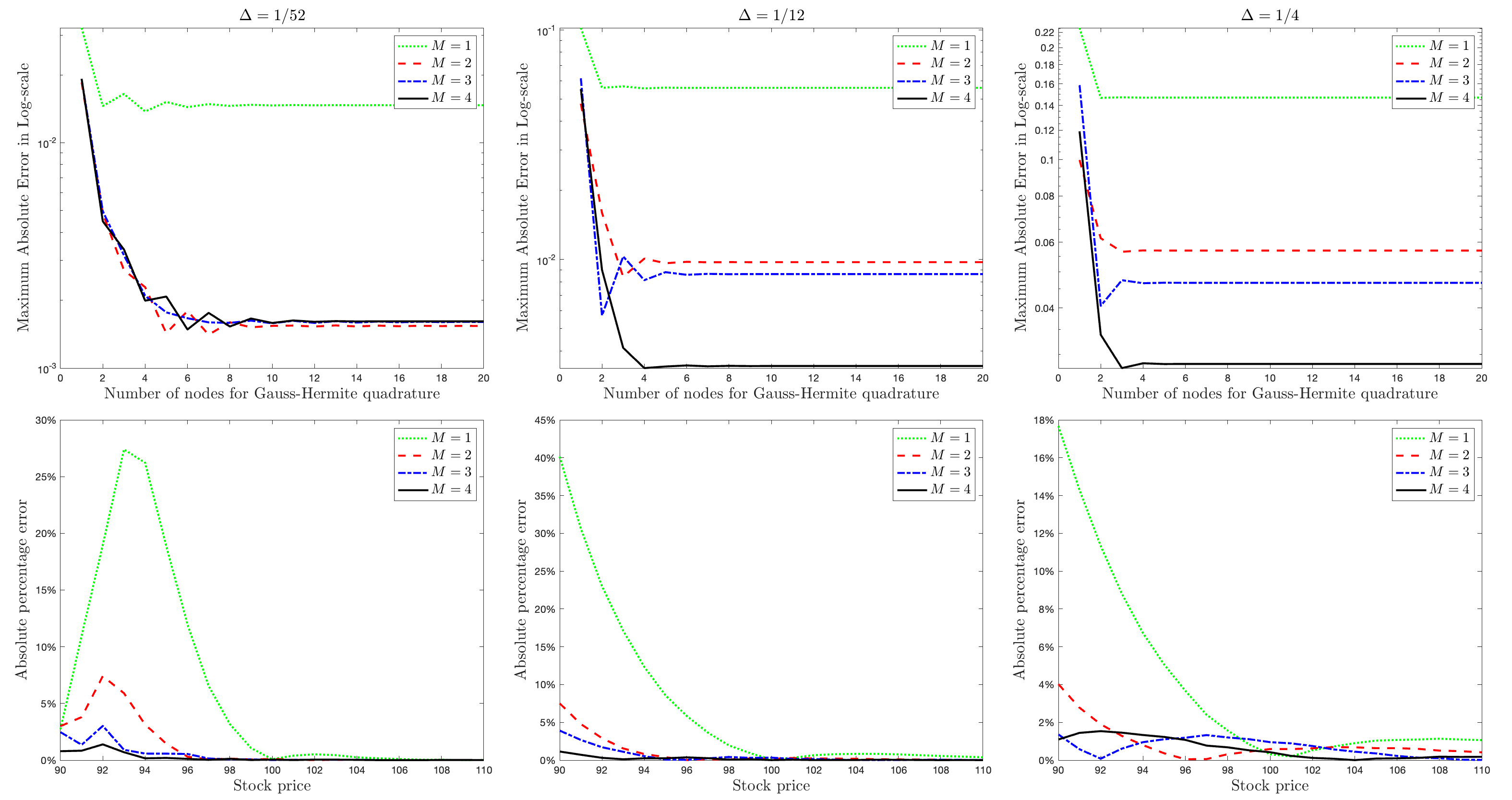
Figure 1: Maximum absolute error (top) and absolute percentage error (bottom) of option price approximations in (5.1)–(5.2) with $\beta=0.5$, $M=1,2,3,4$, $\Delta=1/52,1/12,1/4$, $s=100$, $v=0.0416$

Figure 2 and 3 investigate the numerical performance of our approximation for the call option under the stochastic volatility model (5.1)–(5.2) with the CEV ($\beta=0.8$) and GARCH ($\beta=1$) specifications of variance, respectively. The parameters for the CEV and GARCH specification are from Aït-Sahalia and Kimmel (2007) and Yang and Kanniainen (2016), respectively, but we added or changed the parameters for the jump part, which is the same as in Wan and Yang (2021).

For $\Delta=1/52$ and $\Delta=1/12$, the performances of the approximation for both two models share three patterns arose in the outcome in Figure 1. However, for longer time-to-maturity, $\Delta=1/4$, the higher order of approximation does not guarantee smaller approximation error. In general, the performance of the approximation error is good with shorter maturities and/or $\beta$ takes on a relatively small value.

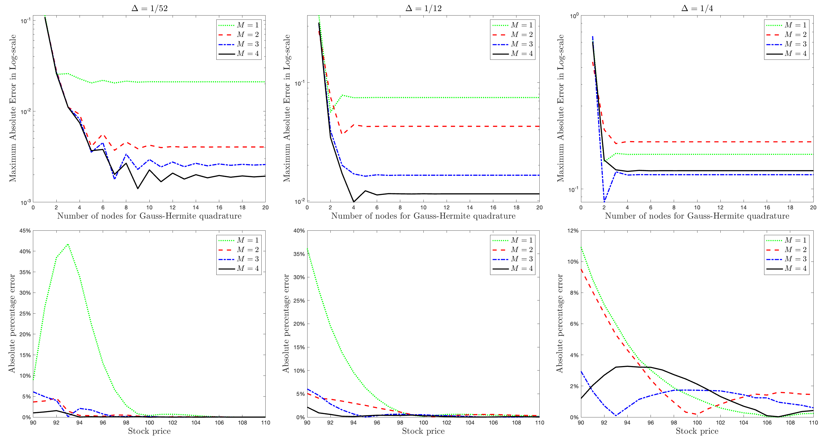
Figure 2: Maximum absolute error (top) and absolute percentage error (bottom) of option price approximations in (5.1)–(5.2) with $\beta=0.8$

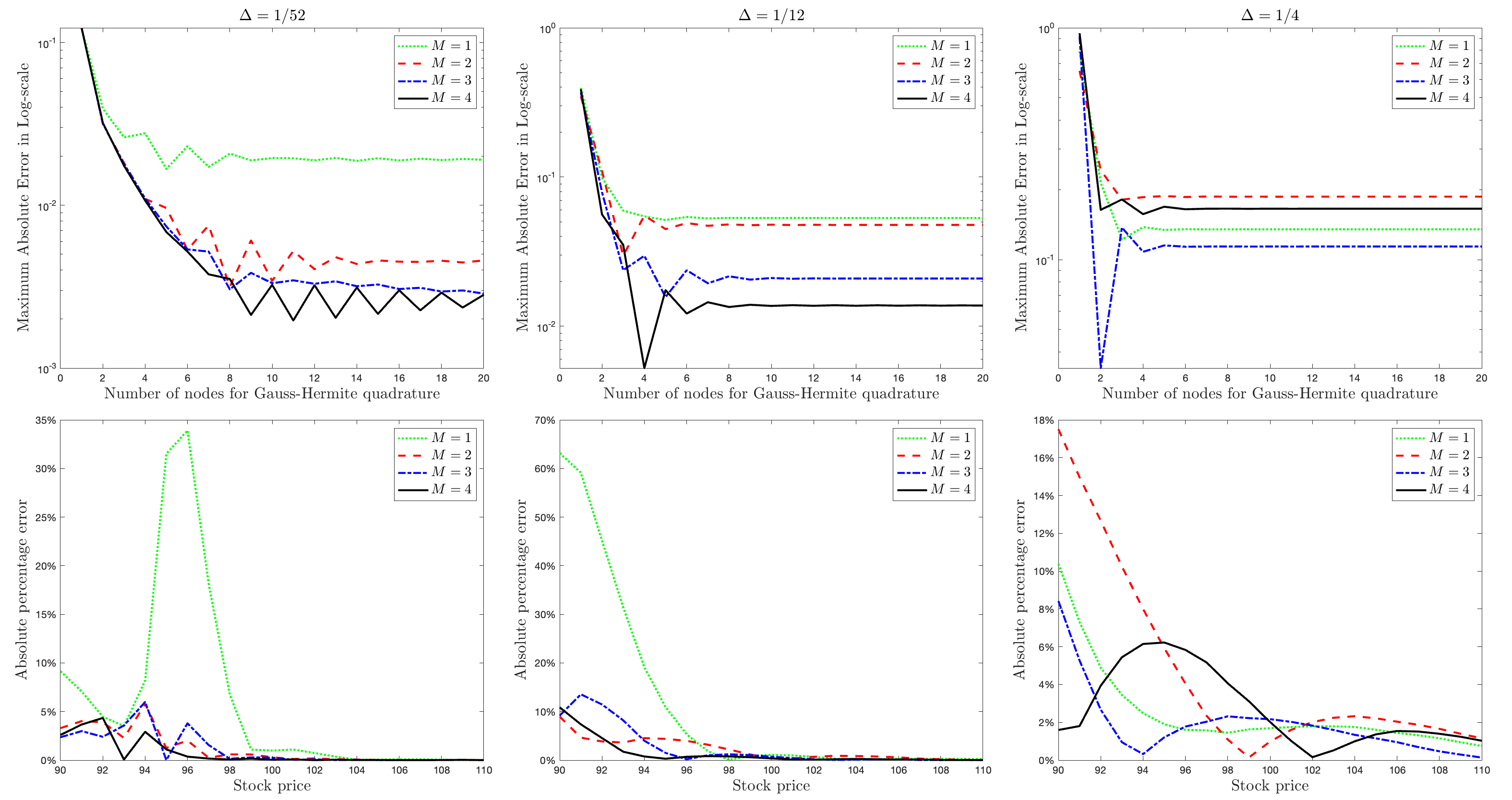
Figure 3: Maximum absolute error (top) and absolute percentage error (bottom) of option price approximations in (5.1)–(5.2) with $\beta=1.0$

5.2 State-dependent jumps

In this subsection, we provide results for the case where the option price is computed under models with state-dependent jump intensities ($\lambda_{1}\neq 0$).

In Figures 4–6, we depict the relative error of the approximation for the same three models considered in the previous subsection, except that now $\lambda_{1}=1,10,30$, when time-to-maturity equal to one month, $\Delta=1/12$. In each figure, from left to right, the state dependency of jump intensity ranges $\lambda_{1}=1,10,30$. Overall, the approximation errors for each of the three models are comparable to that of the same model with state-independent jumps ($\lambda_{1}=0$). Furthermore, the absolute percentage error is smaller for all orders of approximation for larger $\lambda_{1}$. It indicates that the magnitude of $\lambda_{1}$ affects the level of option prices but does not affect the approximation errors. That is, the performance of our approximation is not very sensitive to the degree of state dependence of the jumps as measured by the value of $\lambda_{1}$.

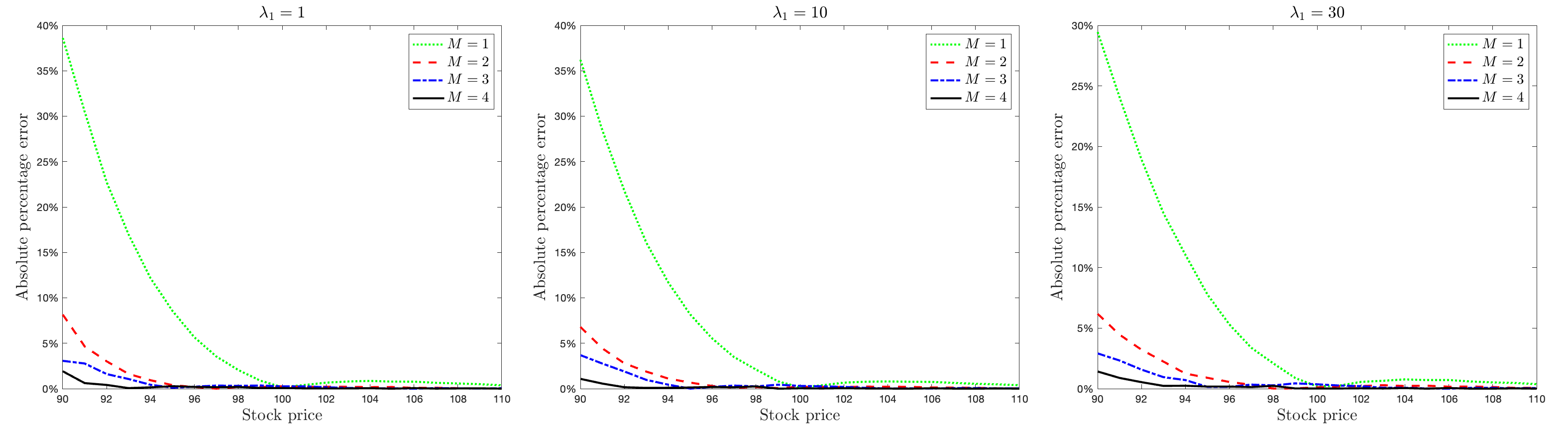
Figure 4: Maximum absolute error (top) and absolute percentage error (bottom) of option price approximations in (5.1)–(5.2) with $\beta=0.5$ and $\lambda_{1}=1$ (left panel), $10$ (middle panel) and $30$ (right panel)

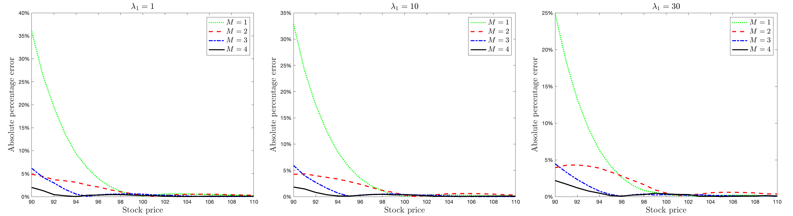
Figure 5: Maximum absolute error (top) and absolute percentage error (bottom) of option price approximations in (5.1)–(5.2) with $\beta=0.8$ and $\lambda_{1}=1$ (left panel), $10$ (middle panel) and $30$ (right panel)

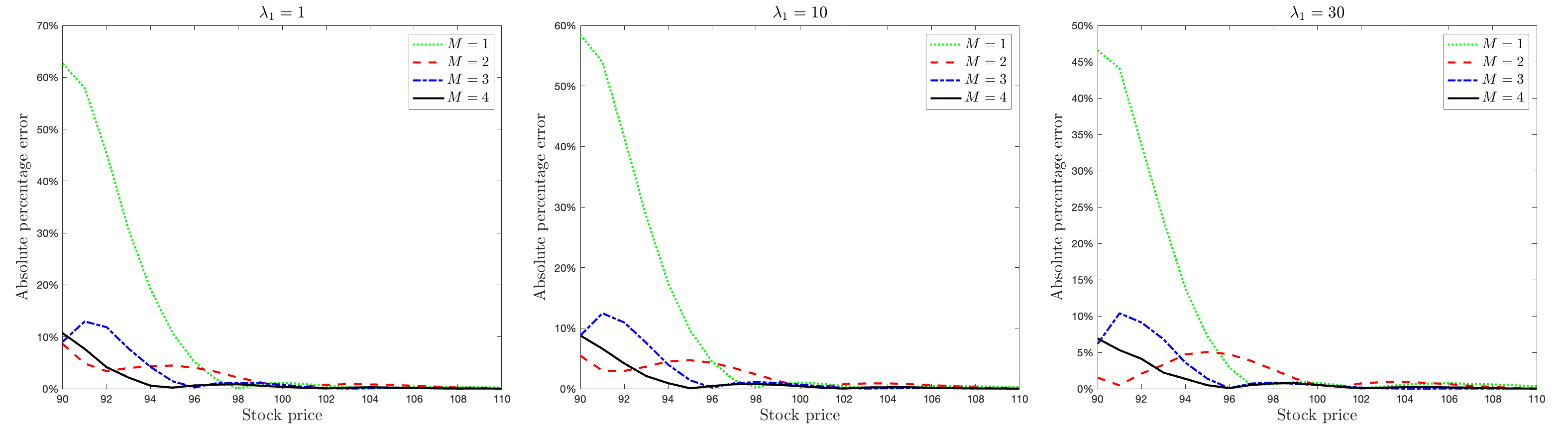
Figure 6: Maximum absolute error (top) and absolute percentage error (bottom) of option price approximations in (5.1)–(5.2) with $\beta=1.0$ and $\lambda_{1}=1$ (left panel), $10$ (middle panel) and $30$ (right panel)

Next, we consider the performance when $v_{t}$ solves the log–volatility model (5.3) with parameters chosen as $\left(r,\delta,\kappa_{V},\alpha_{V},\sigma_{V},\rho\right)=\left(0.0304,0,0.0145,-0.8276,0.1153,-0.6125\right)$ and $\left(\lambda_{0},\mu_{J},\sigma_{J}\right)=\left(0.0137,-0.000125,0.015\right)$; these are the estimates reported in Andersen et al. (2002). Figures 7 and 8 display the relative error of the approximation for the call option under this model for different values of $\Delta$ and $\lambda_{1}$ with $v_{0}=\alpha_{V}=-0.8276$. We see that even for the 2nd order approximation, the approximation error is quite small for all choices of time–to–maturity and $\lambda_{1}$. The plotted errors are now more ragged which we conjecture is due to bigger numerical errors in the Monte Carlo benchmark that we use for comparison.

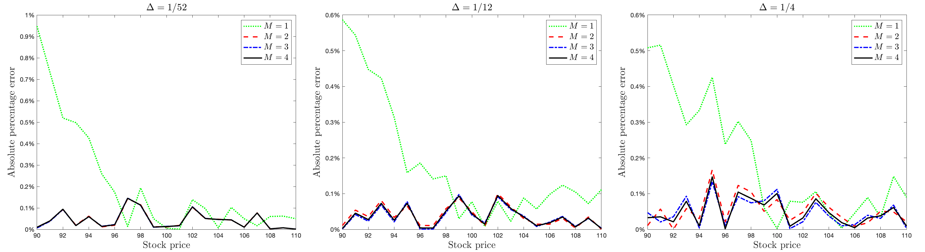
Figure 7: Maximum absolute error (top) and absolute percentage error (bottom) of option price approximations in (5.1) and (5.3) with $\lambda_{1}=1$ and $\Delta=1/52$ (left), 1/12 (center), 1/4 (right)

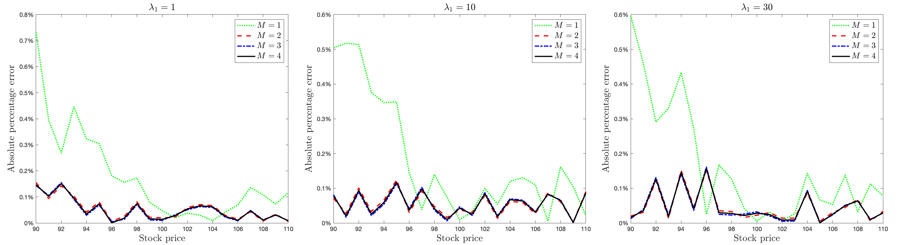
Figure 8: Maximum absolute error (top) and absolute percentage error (bottom) of option price approximations in (5.1) and (5.3) with $\lambda_{1}=1$ (left), 10 (center), 30 (right) and $\Delta=1/12$

5.3 Two-factor affine jump diffusion model

We here wish to examine the robustness of our method when applied to more complex models that go beyond one-factor volatility. We consider the stochastic volatility model with two factors for the volatility used in Filipović et al. (2016). In their specification, the dynamics of $s_{t}$ under the risk–neutral measure are given by

$$\begin{split}ds_{t}&=\left(\mu-v_{t}/2-\lambda\left(v_{t},m_{t}\right)\bar{J}\right)dt+\sqrt{v_{t}}dW_{1t}+\log\left(J_{t}^{S}+1\right)dN_{t},\\ dv_{t}&=\kappa_{V}\left(m_{t}-v_{t}\right)dt+\sigma_{V}\sqrt{v_{t}}\left(\rho dW_{1t}+\sqrt{1-\rho^{2}}dW_{2t}\right)+J_{t}^{V}dN_{t},\\ dm_{t}&=\kappa_{m}\left(\alpha_{m}-m_{t}\right)dt+\sigma_{m}\sqrt{m_{t}}W_{3t},\end{split}$$ (5.4)

where $W_{1}$, $W_{2}$, and $W_{3}$ are mutually independent standard Brownian motions. Compared to the models of the previous subsection, there is a second variance factor $m_{t}$, which represents a stochastic level around which $v_{t}$ reverts. The jump component consists of: (i) $N_{t}$, a Cox process with a bounded intensity function given by $\lambda\left(v,m\right)=\lambda_{0}+\lambda_{1}v+\lambda_{2}m$, and the variance jump size $J^{V}$ is exponentially distributed with parameter $\mu_{J}^{V}=\mathbb{E}\left[J_{t}^{V}\right]$.

Figure 9 reports the performance of our approximation for different times to maturity, and with different numbers of nodes for Gauss-Hermite quadrature. The parameter values we used are estimates in Aït-Sahalia et al. (2020). The performance of the approximation shares the same patterns that we found in Figure 1. It indicates that the performance of the approximation is still very good when we add more factors to the volatility specification.

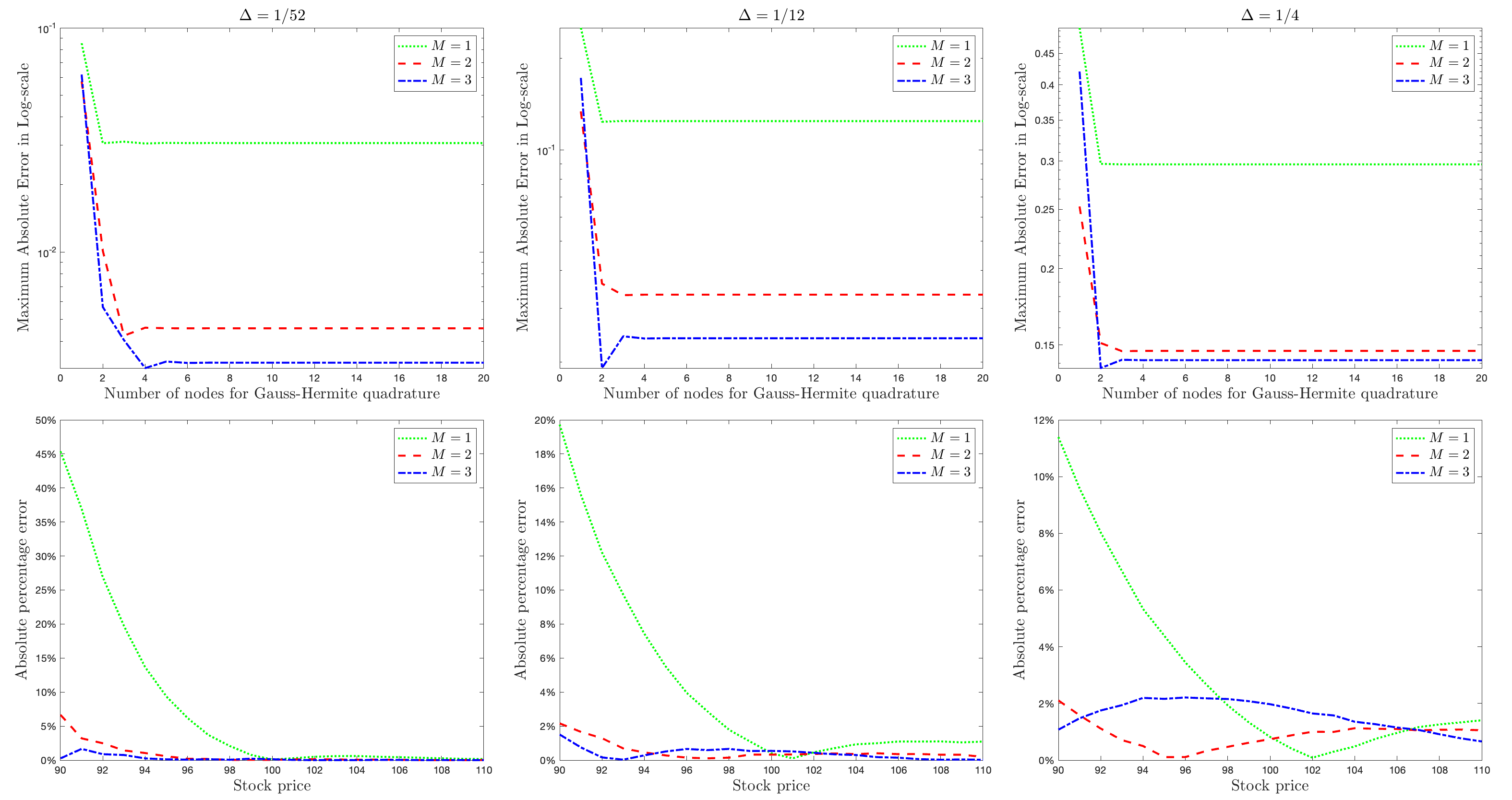
Figure 9: Maximum absolute error (top) and absolute percentage error (bottom) of option price approximations in (5.4) with $\Delta=1/52$, 1/12, 1/4

6 Conclusion

This paper provides a general framework for developing and analyzing series expansions of moments of continuous-time Markov processses, including jump-diffusions. The expansions come in two versions depending on the features of the moment. For ”regular” moments, we provide conditions under which the corresponding expansion will converge towards the actual moments as more terms are added. For the ”smoothed” expansion, no such theoretical guarantees exist: The expansion will eventually become imprecise as the number of terms grows. A numerical study shows that the smoothed expansions still work well in practice when a relatively small number of terms are used in its implementation.

Appendix A Relationship to existing literature

We here first present the proposal of Kristensen and Mele (2011) and show that it falls within the general framework of Section 2. We then proceed to show that the class of series expansions of Kristensen and Mele (2011) contains as special cases the ones of Yang et al. (2019) and Wan and Yang (2021)

Recall the definition of $u_{t}\left(x\right)$ in (2.2) of the motivating jump–diffusion example. To approximate $u_{t}\left(x\right)$, Kristensen and Mele (2011) takes as starting point an auxiliary model on the form

$$dx_{0,t}=\mu_{0}\left(x_{0,t}\right)dt+\sigma_{0}\left(x_{0,t}\right)dW_{t}+J_{0,t}dN_{0,t},$$ (A.1)

where $N_{0,t}$ is a Poisson process with jump intensity $\lambda_{0}\left(x\right)$ and $J_{0,t}$ has density $\nu_{0}\left(\cdot|x\right)$. Let $u_{0,t}\left(x\right)$ be the solution to the problem of interest but now under the auxiliary model,

$$-\partial_{t}u_{0,t}\left(x\right)=\left[A_{0}-r\left(x\right)\right]u_{0,t}\left(x\right),$$ (A.2)

with initial condition $u_{0,0}\left(x\right)=f\left(x\right)$, where $A$ has been replaced by the auxiliary model’s generator, $A_{0}=A_{0,D}+A_{0,J}$, with

$$A_{0,D}f\left(x\right) = \sum_{i=1}^{d}\mu_{0,i}\left(x\right)\partial_{x_{i}}f\left(x\right)+\frac{1}{2}\sum_{i,j=1}^{d}\sigma_{0,ij}^{2}\left(x\right)\partial_{x_{i},x_{j}}^{2}f\left(x\right),$$

$$A_{0,J}f\left(x\right) = \lambda_{0}\left(x\right)\int_{\mathbb{R}^{d}}\left[f\left(x+c\right)-f\left(x\right)\right]\nu_{0}\left(c|x\right)dc.$$

Kristensen and Mele (2011) then subtract (A.2) from (2.7) and, after some straightforward manipulations, arrive at the following PIDE of $\Delta u_{t}\left(x\right)\equiv u_{t}\left(x\right)-u_{0,t}\left(x\right)$:

$$\partial_{t}\Delta u_{t}\left(x\right)=\left[A-r\left(x\right)\right]\Delta u_{t}\left(x\right)+d_{t}\left(x\right).$$ (A.3)

where

$$d_{t}\equiv\left(A-A_{0}\right)u_{0,t}.$$ (A.4)

Since the initial conditions of (LABEL:eq:_PIDE_terminal) and (A.2) are the same, the initial condition of (A.3) becomes $\Delta u_{T}\left(x\right)=0$ which is now smooth and bounded. As with $u_{t}\left(x\right)$, $\Delta u_{t}\left(x\right)$ can be represented as a moment function using Feynman-Kac formula under weak regularity conditions,

$$u_{t}\left(x\right)=u_{0,t}\left(x\right)+\int_{0}^{t}E_{s}d_{s}\left(x\right)ds.$$ (A.5)

The second term on the right-hand side of Eq. (A.5) delivers an exact expression of the difference between $u_{t}\left(x\right)$ and $u_{0,t}\left(x\right)$.

The next step utilizes the smoothness of $d_{t}$ to obtain a Taylor expansion w.r.t. time of this second term. We first develop a power series expansion of the integrand,

$$w_{s}\left(x\right)\equiv E_{s}d_{s}\left(x\right),\text{ \ \ }s\geq 0,$$ (A.6)

at $s=t$ taking the form

$$\hat{w}_{s}\left(x\right)\equiv\sum\limits_{m=0}^{M-1}\frac{\left(s-t\right)^{m}}{m!}\left.\partial_{s}^{m}w_{s}\left(x\right)\right|_{s=t}=\sum\limits_{m=0}^{M-1}\frac{\left(s-t\right)^{m}}{m!}\left(\partial_{t}+A-r\right)^{m}d_{t}\left(x\right).$$

for some $M\geq 1$. This assumes that $\left(\partial_{t}+A-r\right)^{m}d_{t}\left(x\right)$ is well-defined, $1\leq m\leq M$. Combining these last two equations, substituting the resulting expression into (A.5) and evaluating the integral $\int\nolimits_{0}^{t}\hat{w}_{s}\left(x\right)ds$, we obtain the approximation originally proposed in Kristensen and Mele (2011), here extended to the general case of jump–diffusions:

$$\hat{u}_{t}\left(x\right)\equiv u_{0,t}\left(x\right)+\sum\limits_{m=0}^{M-1}\frac{t^{m+1}}{\left(m+1\right)!}\left(-\partial_{t}+A-r\right)^{m}d_{t}\left(x\right),$$ (A.7)

where $\left(-\partial_{t}+A-r\right)^{0}d_{t}\left(x\right)=d_{t}\left(x\right)$.

Finally, observe that an equivalent representation of $\hat{u}_{t}\left(x\right)$ is

$$\hat{u}_{t}\left(x\right)=\sum\limits_{m=0}^{M}\frac{t^{m}}{m!}\left(-\partial_{t}+A-r\right)^{m}u_{0,t}\left(x\right)$$ (A.8)

which follows from combining (A.2) and (A.4) to obtain

$$d_{t}=Au_{0,t}-A_{0}u_{0,t}=Au_{0,t}+\left\{-\partial_{t}u_{0,t}-r\left(x\right)u_{0,t}\right\}=\left(-\partial_{t}+A-r\right)u_{0,t}.$$

We recognize (A.8) as a special case of the general proposal in (2.16).

Next, we demonstrate that the above class of series expansions include as special cases the approximate transition densities and option prices proposed in Yang et al. (2019) and Wan and Yang (2021). With $r=0$ and $f\left(x\right)=\delta\left(y-x\right)$, (A.8) becomes

$$\hat{p}_{t}\left(y|x\right)=\sum\limits_{m=0}^{M}\frac{t^{m}}{m!}\left(-\partial_{t}+A\right)^{m}p_{0,t}\left(y|x\right),$$ (A.9)

where $p_{0,t}\left(y|x\right)$ is the transition density of the auxiliary model. Now, let us first consider the transition density expansion developed in Yang et al. (2019) for pure diffusions ($A_{J}=0$). Inspecting the expansion presented in eq. (10) of their paper, we recognize it to be identical to above when $p_{0,t}$ is chosen as in eq. (3.4) with $\sigma_{0}=\sigma\left(x\right)$. Thus, Yang et al. (2019) is a special case of Kristensen and Mele (2011). This somehow went unnoticed by the authors and we here clarify the connection between the two papers. Second, consider the expansion of the transition density in Wan and Yang (2021) in the pure diffusion case. As explained by the authors themselves, the preferred version of the expansion used in this paper is the same as the series expansion of Yang et al. (2019) when $\mu_{0}=0$ in the auxiliary BM model. And so the pure diffusion version of Wan and Yang (2021) is also a special case of Kristensen and Mele (2011).

Next, we show that the expansion of option prices developed in Wan and Yang (2021) is again a special case of Kristensen and Mele (2011). Setting $r\left(x\right)=0$ and $f\left(x\right)=\left(\exp\left(x_{1}\right)-K\right)^{+}$ and using as auxiliary model (3.3), $\hat{u}_{t}\left(x\right)$ as given in (A.8) delivers an expansion of the expected pay-off of a European option where $u_{0,t}\left(x\right)$ is now the pay-off function under the Black–Scholes model. To connect this option price approximation with the corresponding proposal of Wan and Yang (2021), observe that $u_{0,t}\left(x\right)=\int f\left(y\right)p_{0,t}\left(y|x\right)dy$, where $p_{0,t}\left(y|x\right)$ is given in (3.4). Substituting this into (A.8) and changing the order of integration and differentiation yields

$$\hat{u}_{t}(x) = \sum\limits_{m=0}^{M}\frac{t^{m}}{m!}\left(-\partial_{t}+A\right)^{m}\int f\left(y\right)p_{0,t}\left(y|x\right)dy$$ (A.10)

$$= \int f\left(y\right)\left\{\sum\limits_{m=0}^{M}\frac{t^{m}}{m!}\left(-\partial_{t}+A\right)^{m}p_{0,t}\left(y|x\right)\right\}dy$$

$$= \int f\left(y\right)\hat{p}_{t}\left(y|x\right)dy,$$

where $\hat{p}_{t}\left(y|x\right)$ is the density approximation we arrived at in (A.9). Thus, for simple moment functions, such as the ones appearing in European option prices with constant interest rates, the expansion of Kristensen and Mele (2011) is equivalent to first developing the corresponding expansion for the transition density and then using this to compute the relevant moment. However, in practice, it is easier to directly employ (A.8) with $u_{0,t}$ chosen as the pay-off under the Black–Scholes model since this avoids having to compute the integral $\int f\left(y\right)\hat{p}_{t}\left(y|x\right)dy$ after developing the expansion of the transition density.

Let us consider Wan and Yang (2021)’s proposal for option pricing approximation: They take as starting point that the pay-off can be written as $u_{t}(x)=\int f\left(y\right)p_{t}\left(y|x\right)dy,$and then replace $p_{t}\left(y|x\right)$ by the approximation given in (A.9) with auxiliary model chosen as Brownian motion with drift. As we just demonstrated in (A.10), this is identical to the approximation developed in Kristensen and Mele (2011) when the auxiliary model is chosen as the Black–Scholes model since the log–price in this case follows a Brownian Motion with drift. Thus, the option price approximation of Wan and Yang (2021) is again a special case of Kristensen and Mele (2011).

Appendix B Extension to time-inhomogenous problems

We here present the extension of our method to handle time–inhomogenous models and problems where no closed-form solution is available to (A.2). As motivating example, consider the following extended version of the model in (2.1):

$$dx_{t}=\mu_{t}\left(x_{t}\right)dt+\sigma_{t}\left(x_{t}\right)dW_{t}+J_{t}\left(x_{t}\right)dN_{t},$$ (B.1)

where now $\lambda_{t}\left(x\right)$, $\mu_{t}\left(x\right)$, $\sigma_{t}\left(x\right)$ and $\nu_{t}\left(x_{t}\right)$ are now allowed to vary with $t$. This in turn implies that the corresponding generator is also time–varying, $A_{t}f\left(x\right)=A_{D,t}f\left(x\right)+A_{J,t}f\left(x\right)$, where

$$A_{D,t}f\left(x\right) = \sum_{i=1}^{d}\mu_{i,t}\left(x\right)\partial_{x_{i}}f\left(x\right)+\frac{1}{2}\sum_{i,j=1}^{d}\sigma_{ij,t}^{2}\left(x\right)\partial_{x_{i},x_{j}}^{2}f\left(x\right),$$

$$A_{J,t}f\left(x\right) = \lambda_{t}\left(x\right)\int_{\mathbb{R}^{d}}\left[f\left(x+c\right)-f\left(x\right)\right]\nu_{t}\left(c\right)dc.$$

We are interested in computing $u_{s,t}\left(x\right)$ defined as

$$u_{s,t}\left(x\right)=E_{s,t}f\left(x\right),\text{ \ \ }0\leq s\leq t,$$ (B.2)

where

$$\left(s,t,f\right)\mapsto E_{s,t}f\left(x\right)\equiv\mathbb{E}\left[\left.\exp\left(-\int\nolimits_{s}^{t}r\left(x_{u}\right)du\right)f\left(x_{t}\right)\right|x_{s}=x\right].$$ (B.3)

Due to the time–inhomogeneity, the operator $E_{s,t}f\left(x\right)$ is now indexed by two time variables, $s$ and $t$. At the same time, for any fixed value of $s\geq 0$, $\left(t,f\right)\mapsto E_{s,t}f\left(x\right)$ remains a semi–group when $\mathcal{F}$ is chosen suitably. Most of the ideas and results from Sections 2–4 therefore carry over to the time–inhomogenous case with only minor differences. Below, we present the series expansion and explain how the theory applies to this.

We take as starting point a given $\left(s,t,f\right)\mapsto E_{s,t}f\left(x\right)$ where, for any given $s\geq 0$, $\left(t,f\right)\mapsto E_{s,t}f\left(x\right)$ is assumed to be semi–group on some funtion space $\left(\mathcal{F},\left\|\cdot\right\|_{\mathcal{F}}\right)$. In the following, we keep $s\geq 0$ fixed. We denote by $\mathcal{D}\left(B_{s}\right)$ the set of functions $f\in\mathcal{F}$ for which there exists $g_{s}\in\mathcal{F}$ such that, for each $t\geq 0$,

$$E_{s,t}f\left(x\right)=f\left(x\right)+\int_{s}^{t}E_{s,u}g_{s}\left(x\right)du,$$ (B.4)

and we write $B_{s}f\left(x\right):=g_{s}\left(x\right)$ and call $B_{s}$ the (extended) generator of $E_{s,t}$. In the motivating example above, it is easily shown by Ito’s Lemma that $B_{t}=A_{t}-r$ on the space

$$\mathcal{D}_{0}\left(B_{s}\right):=\left\{f\in\mathcal{C}^{2}\cap\mathcal{F}:E_{s,t}\left|f\right|\text{ and }E_{s,t}\left\|\frac{\partial f}{\partial x}\sigma_{s}\right\|^{2}\text{ exist for all }t>0\right\}\subseteq\mathcal{D}\left(B_{s}\right).$$

For any regular function $f$, regular in the sense that $f\in\mathcal{D}\left(B_{s}^{M}\right)$, we have

$$\partial_{t}u_{s,t}\left(x\right)=B_{t}^{m}u_{s,t}\left(x\right),\text{ \ }t>0,$$ (B.5)

c.f. Rüschendorf et al. (2016), which corresponds to the so–called forward equation. Thus, in this case the following is a valid series expansion of $u_{s,t}\left(x\right)$:

$$\hat{u}_{s,t}\left(x\right)=\sum\limits_{m=0}^{M}\frac{\left(t-s\right)^{m}}{m!}B_{s}^{m}f\left(x\right).$$ (B.6)

If $f$ is irregular, so that $f\notin\mathcal{D}\left(B_{s}\right)$, we introduce a smoothed version of it, $u_{0,s,t}\left(x\right)$ which is assumed to satisfy:

A.0’

(i) $\lim_{t\rightarrow s^{+}}u_{0,s,t}\left(x\right)=f\left(x\right)$ and (ii) $u_{0,s,t}\in\mathcal{D}\left(\left(\partial_{t}\right)^{M_{1}}\right)\cap\mathcal{D}\left(B_{s}^{M_{2}}\right)$ for some $M_{1},M_{2}\geq 1$.

Following the same steps as in the time–homogenous case of Section 2, we obtain the following series expansion:

$$\hat{u}_{s,t}\left(x\right)=\sum\limits_{m=0}^{M}\frac{\left(t-s\right)^{m}}{m!}\left(B_{s}-\partial_{t}\right)^{m}u_{0,s,t}\left(x\right).$$ (B.7)

Appendix C Proofs

Proof of Theorem 4.2. Use eq. (4.3) together with $E_{s}E_{t}=E_{s+t}=E_{t}E_{s}$ to obtain

$$E_{t}u_{s}\left(x\right)=u_{s}\left(x\right)+\int_{0}^{t}E_{s+w}\left(Bf\right)\left(x\right)dw=\int_{0}^{t}E_{w}\left(E_{s}\left(Bf\right)\right)\left(x\right)dw.$$

The second part of the theorem is obtained by taking derivatives w.r.t. $s$ on both sides of (4.3) and using that the right-hand side derivative equals $E_{s}\left(Bf\right)\left(x\right)=Bu_{s}\left(x\right)$ if this function is continuous w.r.t $s$ from the right.    

Proof of Theorem 4.4. We expand $t\mapsto E_{t}f\left(x\right)$ around $E_{0}f\left(x\right)=f\left(x\right)$ recursively: First rewrite (4.3) as

$$E_{t}f\left(x\right)=f\left(x\right)+\int_{0}^{t}E_{t_{1}}\left(Bf\right)\left(x\right)dt_{1}.$$ (C.1)

Since $Bf\in\mathcal{D}\left(B\right)$ by assumption, we can apply (C.1) again to $E_{t_{1}}\left(Bf\right)\left(x\right)$ yielding

$$E_{t_{1}}\left(Af\right)\left(x\right)=Bf\left(x\right)+\int_{0}^{t_{1}}E_{t_{2}}\left(B^{2}f\right)\left(x\right)dt_{2}.$$

Substitute the right-hand side of the last equation into (C.1) to obtain

$$E_{t}f\left(x\right) = f\left(x\right)+\int_{0}^{t}\left\{Bf\left(x\right)+\int_{0}^{t_{1}}E_{t_{2}}\left(B^{2}f\right)\left(x\right)dt_{2}\right\}dt_{1}$$

$$= f\left(x\right)+tBf\left(x\right)+\int_{0}^{t}\int_{0}^{t_{1}}E_{t_{2}}\left(B^{2}f\right)\left(x\right)dt_{2}dt_{1}.$$

Repeating this argument $M$ more times yields the claimed result.    

Proof of Theorem 4.5. By definition, $\left\|B^{m}f\right\|_{\mathcal{F}}/m!\leq 1/T_{0}^{m}$. Thus,

$$\left\|u_{t}-\hat{u}_{t}\right\|_{\mathcal{F}}\leq\sum_{m=M+1}^{\infty}\frac{t^{m}}{m!}\left\|B^{m}f\left(x\right)\right\|_{\mathcal{F}}\leq\sum_{m=M+1}^{\infty}\left(\frac{t}{T_{0}}\right)^{m}=\frac{\left(t/T_{0}\right)^{M+1}}{1-t/T_{0}}\rightarrow 0.$$

 

Proof of Theorem 4.7. The first part follows from Theorem 2.5.2 of Pazy (1983). To show the second part, recall the definition of radius of convergence $T_{0}$ in (4.8). To bound the right hand side of (4.8), first use that $f\left(x\right)=E_{\tau_{0}}g\left(x\right)$ and that $A$ and $E_{\tau_{0}}$ commute to obtain $\left\|B^{m}f\right\|_{\mathcal{F}}=\left\|\left(BE_{\tau_{0}/m}\right)^{m}g\right\|_{\mathcal{F}}\leq\left\|BE_{\tau_{0}/m}\right\|_{\mathrm{op}}^{m}\left\|g\right\|_{\mathcal{F}}$. Next, due to (4.9)–(4.10), we can apply part (d) of Theorem 2.5.2 of Pazy (1983) yielding $\left\|BE_{\tau_{0}/m}\right\|_{\mathrm{op}}^{m}\leq\left(C_{A}m/\tau_{0}\right)^{m}$. In total,

$$\left\|B^{m}f\right\|_{\mathcal{F}}/m!\leq\left\{\left(\frac{C_{A}}{\tau_{0}}\right)^{m}m^{m}/m!\right\}^{1/m}\left\|g\right\|_{\mathcal{F}}^{1/m}\leq\left(\frac{C_{A}e}{\tau_{0}}\right)\left\|g\right\|_{\mathcal{F}}^{1/m},$$

and we conclude that $T_{0}\geq\tau_{0}/\left(C_{A}e\right)$.    

Proof of Corollary 4.9. With the function space being a Hilbert space, we are able to introduce the adjoint $A^{\ast}$ of the operator $A$ with corresponding semigroup $E_{t}^{\ast}=e^{A^{\ast}t}$. If $x_{t}$ indeed is reversible in the sense that $A=A^{\ast}$ then $\sigma\left(A\right)\subseteq(-\infty,0]$ and so (4.9) is satisfied. (c.f. eq. 5.8 in Hansen and Scheinkman (1995)). Moreover, by the Spectral Mapping Theorem (Rudin (1973), Theorem 10.28), the spectrum of the resolvent satisfies

$$\sigma\left(R\left(\lambda\right)\right)\backslash\left\{0\right\}=\left(\lambda-\sigma\left(A\right)\right)^{-1}=\left\{\frac{1}{\lambda-w}:w\in\sigma\left(A\right)\right\}$$

Since $A$ is self-adjoint so is $R\left(\lambda\right)$ for any $\lambda\notin\sigma\left(A\right)$. Thus,

$$\left\|R\left(\lambda\right)\right\|_{\mathrm{op}}=\max_{w\in\sigma\left(R(\lambda\right))}\left|w\right|=\max_{w\in\sigma\left(A\right)}\frac{1}{\left|\lambda-w\right|}\leq\max_{w\leq 0}\frac{1}{\left|\lambda-w\right|}=\frac{1}{\left|\lambda\right|},$$

and so (4.10) is satisfied.    

Proof of Theorem 4.10. For any $f\in\mathcal{F}_{0}$,

$$\left\|A_{D}f\right\|_{\mathcal{F}_{0}} \leq \sum_{i=1}^{d}\left\|\mu_{i}\right\|_{\mathcal{F}}\left\|\frac{\partial f}{\partial x_{i}}\right\|_{\mathcal{F}}+\frac{1}{2}\sum_{i,j=1}^{d}\left\|\sigma_{ij}^{2}\right\|_{\mathcal{F}}\left\|\frac{\partial^{2}f}{\partial x_{i}\partial x_{j}}\right\|_{\mathcal{F}}$$

$$\leq \left(\sum_{i=1}^{d}\left\|\mu_{i}\right\|_{\mathcal{F}_{0}}+\frac{1}{2}\sum_{i,j=1}^{d}\left\|\sigma_{ij}^{2}\right\|_{\mathcal{F}_{0}}\right)\left\|f\right\|_{\mathcal{F}_{0}}$$

$$= :\bar{A}\left\|f\right\|_{\mathcal{F}_{0}},$$

where $\bar{A}<\infty$ under the assumptions of the theorem. Thus, $\left\|A\right\|_{\mathrm{op}}=\sup_{\left\|f\right\|_{\mathcal{F}_{0}}\leq 1}\left\|Af\right\|_{\mathcal{F}_{0}}<\infty$ and so $A:\mathcal{F}_{0}\mapsto\mathcal{F}_{0}$ is a bounded operator. This in turn implies that $\sum_{m=0}^{\infty}\frac{t^{m}}{m!}A^{m}f\left(x\right)$ is a well-defined representation of $w_{t}\left(x\right)$ for any $f\in\mathcal{F}_{0}$ and so the power series approximation is consistent. In particular,

$$\left\|\hat{w}_{t}-w_{t}\right\|_{\mathcal{F}_{0}}\leq\frac{t^{M+1}}{\left(M+1\right)!}\left\|A^{M+1}f\right\|_{\mathcal{F}_{0}}\leq\frac{\left(t\bar{A}\right)^{M+1}}{\left(M+1\right)!}\left\|f\right\|_{\mathcal{F}_{0}}.$$

 

Proof of Theorem 4.11. The first part follows from Theorem 1.1 in Escauriaza et al. (2017). For the second part, First note that $w_{0,t}\left(x\right)=E_{0,t+\tau_{0}}g\left(x\right)$. Now, by Theorem 1.1 in Escauriaza et al. (2017), $\left|\left.\partial_{t}^{m}w_{0,t}\right|_{t=0}\right|\leq C\left(\rho\tau_{0}\right)^{-m}m!$, for all $x\in\mathcal{X}_{0}$, for some constant $\rho=\rho\left(B,d\right)\in(0,1]$. This in turn implies that the power series expansion will converge with radius of convergence bounded by

$$T_{0}^{-1}=\lim\sup_{m\rightarrow\infty}\left\{\frac{1}{m!}\left\|\left.\partial_{t}^{m}w_{0,t}\right|_{t=0}\right\|_{\mathcal{F},0}\right\}^{1/m}\leq\frac{1}{\rho\tau_{0}}.$$

References

- Aït-Sahalia (2002) Aït-Sahalia, Y. (2002). Maximum likelihood estimation of discretely sampled diffusions: A closed-form approximation approach. Econometrica 70(1), 223–262.
- Aït-Sahalia (2008) Aït-Sahalia, Y. (2008). Closed-form likelihood expansions for multivariate diffusions. The Annals of Statistics 36(2), 906–937.
- Aït-Sahalia et al. (2010) Aït-Sahalia, Y., L. P. Hansen, and J. A. Scheinkman (2010). Operator methods for continuous-time markov processes. In Handbook of Financial Econometrics: Tools and Techniques, pp. 1–66. Elsevier.
- Aït-Sahalia et al. (2020) Aït-Sahalia, Y., M. Karaman, and L. Mancini (2020). The term structure of equity and variance risk premia. Journal of Econometrics 219(2), 204–230. Annals Issue: Econometric Estimation and Testing: Essays in Honour of Maxwell King.
- Aït-Sahalia and Kimmel (2007) Aït-Sahalia, Y. and R. L. Kimmel (2007). Maximum likelihood estimation of stochastic volatility models. Journal of Financial Economics 83(2), 413–452.
- Ames (1992) Ames, W. (1992). Numerical Methods for Partial Differential Equations. Academic Press.
- Andersen et al. (2002) Andersen, T. G., L. Benzoni, and J. Lund (2002). An empirical investigation of continuous-time equity return models. The Journal of Finance 57(3), 1239–1284.
- Bakshi et al. (2006) Bakshi, G., N. Ju, and H. Ou-Yang (2006). Estimation of continuous-time models with an application to equity volatility dynamics. Journal of Financial Economics 82(1), 227–249.
- Beskos et al. (2009) Beskos, A., O. Papaspiliopoulos, and G. Roberts (2009). Monte Carlo maximum likelihood estimation for discretely observed diffusion processes. The Annals of Statistics 37(1), 223 – 245.
- Björk (2009) Björk, T. (2009). Arbitrage Theory in Continuous Time. Oxford University Press.
- Brandt and Santa-Clara (2002) Brandt, M. W. and P. Santa-Clara (2002). Simulated likelihood estimation of diffusions with an application to exchange rate dynamics in incomplete markets. Journal of Financial Economics 63(2), 161–210.
- Cont and Tankov (2003) Cont, R. and P. Tankov (2003, dec). Financial Modelling with Jump Processes. Chapman and Hall/CRC.
- Davies (2007) Davies, E. B. (2007). Linear Operators and their Spectra. Cambridge University Press.
- Durham and Gallant (2002) Durham, G. B. and A. R. Gallant (2002). Numerical techniques for maximum likelihood estimation of continuous-time diffusion processes. Journal of Business & Economic Statistics 20(3), 297–338.
- Elerian et al. (2001) Elerian, O., S. Chib, and N. Shephard (2001). Likelihood inference for discretely observed nonlinear diffusions. Econometrica 69(4), 959–993.
- Eraker (2004) Eraker, B. (2004). Do stock prices and volatility jump? reconciling evidence from spot and option prices. The Journal of Finance 59(3), 1367–1403.
- Escauriaza et al. (2017) Escauriaza, L., S. Montaner, and C. Zhang (2017, jan). Analyticity of solutions to parabolic evolutions and applications. SIAM Journal on Mathematical Analysis 49(5), 4064–4092.
- Ethier and Kurtz (1986) Ethier, S. N. and T. G. Kurtz (1986). Markov Processes. John Wiley & Sons, Inc.
- Filipović et al. (2016) Filipović, D., E. Gourier, and L. Mancini (2016). Quadratic variance swap models. Journal of Financial Economics 119(1), 44–68.
- Filipović et al. (2013) Filipović, D., E. Mayerhofer, and P. Schneider (2013, oct). Density approximations for multivariate affine jump-diffusion processes. Journal of Econometrics 176(2), 93–111.
- Giesecke et al. (2018) Giesecke, K., A. Shkolnik, G. Teng, and Y. Wei (2018). Numerical solution of jump-diffusion sdes. Available at SSRN 2298701.
- Hansen and Scheinkman (1995) Hansen, L. P. and J. A. Scheinkman (1995). Back to the future: Generating moment implications for continuous-time markov processes. Econometrica 63(4), 767–804.
- Hansen et al. (1998) Hansen, L. P., J. A. Scheinkman, and N. Touzi (1998). Spectral methods for identifying scalar diffusions. Journal of Econometrics 86(1), 1–32.