Quantifying the biomimicry gap in biohybrid systems

Abstract

Biohybrid systems in which robotic lures interact with animals have become compelling tools for probing and identifying the mechanisms underlying collective animal behavior. One key challenge lies in the transfer of social interaction models from simulations to reality, using robotics to validate the modeling hypotheses. This challenge arises in bridging what we term the “biomimicry gap”, which is caused by imperfect robotic replicas, communication cues and physics constrains not incorporated in the simulations that may elicit unrealistic behavioral responses in animals. In this work, we used a biomimetic lure of a rummy-nose tetra fish (Hemigrammus rhodostomus) and a neural network (NN) model for generating biomimetic social interactions. Through experiments with a biohybrid pair comprising a fish and the robotic lure, a pair of real fish, and simulations of pairs of fish, we demonstrate that our biohybrid system generates high-fidelity social interactions mirroring those of genuine fish pairs. Our analyses highlight that: 1) the lure and NN maintain minimal deviation in real-world interactions compared to simulations and fish-only experiments, 2) our NN controls the robot efficiently in real-time, and 3) a comprehensive validation is crucial to bridge the biomimicry gap, ensuring realistic biohybrid systems.

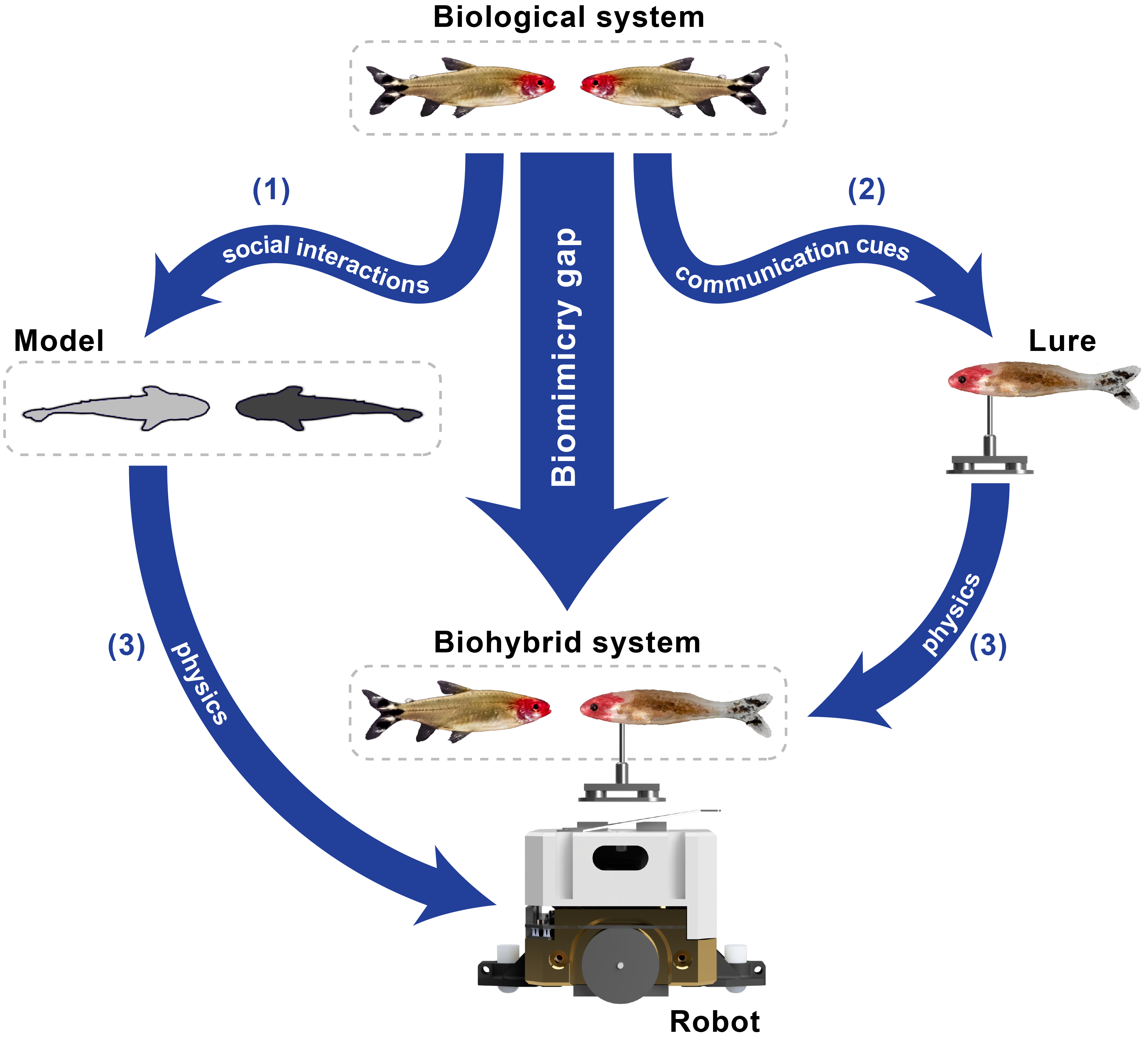
Figure 1: Illustration of the sources of the biomimicry gap. (1) The modeling phase may introduce a first source of discrepancy between the effect of social interactions on the swimming patterns in the model and the ones observed in real fish. (2) A second source of discrepancy between the visual appearance of the lure and that of a real fish might introduce imperfect communication cues and elicit unrealistic behavioral responses from neighboring organisms. (3) Finally, a third source of discrepancy between the characteristics of the movement produced by the model and its realization by the lure occurs when the numerical model is transferred to real-world scenarios due to the physics constrains that were not accounted for in the model. H. rhodostomus photo was taken by David Villa ScienceImage/CBI/CNRS, Toulouse.

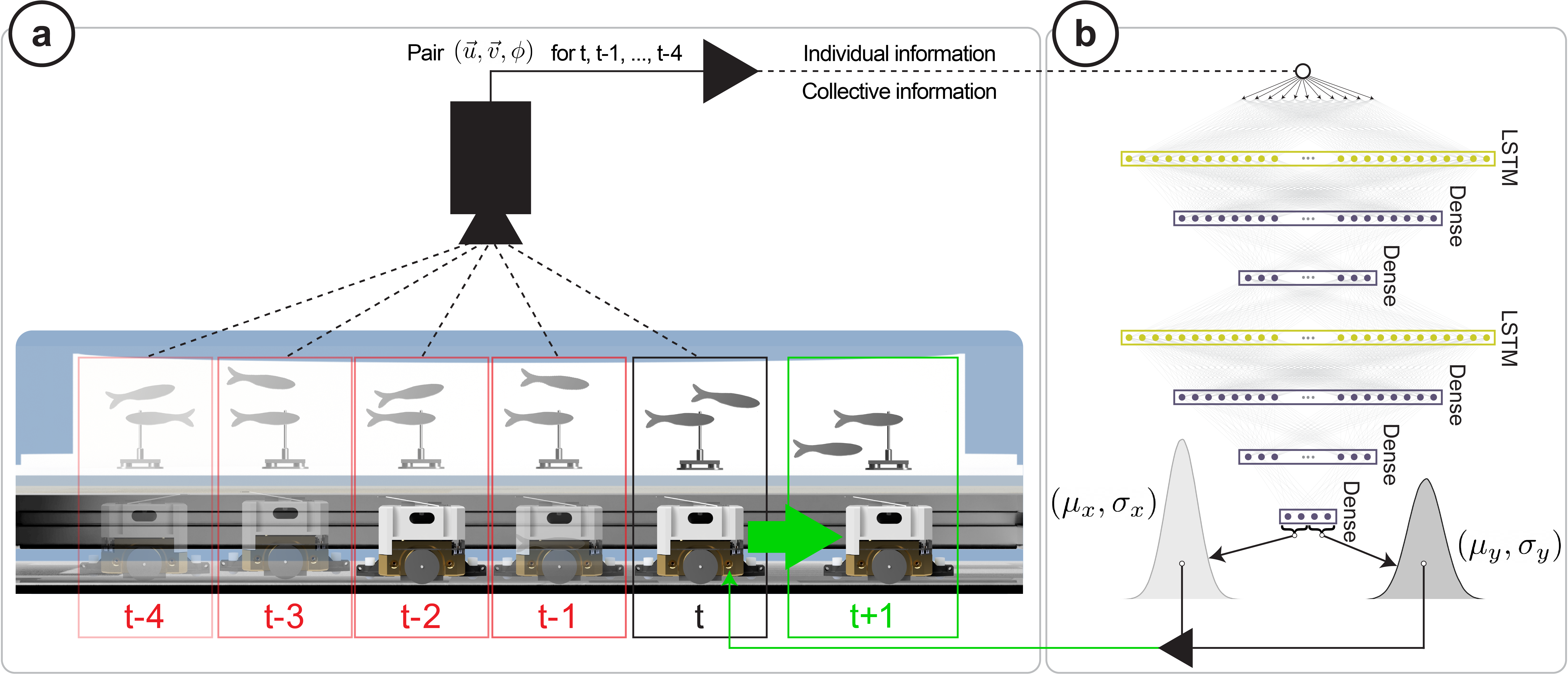
Figure 2: Closed-loop robot control with Deep Learning Interaction (DLI) model. (a) We use the top setup camera to track all agents (fish and/or lure) in real-time, and store unique trajectories for each agent. A $5\times 11$ vector of individual and collective states, spanning 5 timesteps is fed to the DLI. (b) The DLI outputs two acceleration distributions, one for each Cartesian component. Then, the accelerations are converted to desired speed and position for $t+1$ and communicated to the robot.

I Introduction

Robot-animal interactions have been increasingly gaining momentum as means to study collective behavior. Biohybrid systems, composed of living organisms and artificial agents, are particularly compelling as they enable researchers to investigate the way animals respond to controlled interactions. This is typically achieved through autonomous robotic devices equipped with species-specific communication channels, which can be employed to evoke responses in a biomimetic or non-biomimetic manner [41]. Robots offer the advantage of conducting repetitive and repeatable experiments, even when driven by complex behavioral models. This is particularly important in the context of social interactions, which encompass considerable complexity when scaling from short-term interactions at the individual level to long-term emergent collective patterns.

Social fish species, such as the rummy-nose tetra (Hemigrammus rhodostomus) and zebrafish (Danio rerio), are frequently selected for these studies due to the intricacy of their short- and long-term interactions and their suitability for laboratory environments [9, 41], as well as the abundance of general knowledge about their behavior, genetics, and housing conditions [33, 31, 48, 19, 22]. As a matter of fact, many fish-robot systems have been proposed to investigate various aspects of fish behavior, employing behavioral models with diverse degrees of detail and realistic features, and typically relying on analytical modeling approaches based on observation of fish interaction [21, 47, 30, 6, 29, 7, 39, 34, 42, 44, 17, 16, 15, 19]. Concurrently, machine learning-based modeling approaches have gained more interest [36, 23, 20, 13, 14], but only a handful have been tested in real-time with a robotic device [13]. These machine learning approaches are usually intended to study collective behavior by predicting motion in simulations alone [23, 20, 13], while the latter [14] only evaluate instantaneous group-level quantities in the short-term timescale.

A few flocking models for fish behavior, analytical or machine learning, have been evaluated in extended simulations to study long-term emergent collective behavior [19, 11, 36]; however, these models have not been tested and validated in biohybrid groups. Conversely, numerous models have been implemented on robotic devices without being tested in simulations [2, 8, 15, 17, 16, 14, 34]. Furthermore, the majority of these studies involve robot experiments lasting no more than 30 minutes, with the resulting interactions typically assessed solely in the short term. Consequently, none of these models have been stringently benchmarked on both short- and long-term timescales within both simulation and fish-robot biohybrid experiments. In fact, previous research indicates that certain models may yield satisfactory biomimetic outcomes in the short term while failing to reproduce emergent dynamics accurately on longer time scales [36].

Moreover, the transfer of computer models of social interactions into robot controllers that operate in real situations involving animals is not simple and can generate a discrepancy with their numerical simulation, akin to the reality gap observed when transferring simulated robot controllers to real-world applications [32]. As depicted in Fig. 1, many sources of discrepancy can combine and feed this gap: 1) subtle behavioral patterns that social interaction models fail to capture, 2) physics related to the operation of the robot in real life that were not accounted for, and 3) the extent of biomimicry exhibited by artificial lures [43, 35]. We refer to the cumulative effect of these discrepancies with the term “biomimicry gap”. Therefore, the biomimicry gap is an inherent aspect of the multifaceted, cross-domain process of creating biohybrid groups composed of animals and robots. To the best of our knowledge, the feasibility of bridging this biomimicry gap — achieved by conducting extended experiments in both simulated and real-world environments, and comparing their results — has yet to be conclusively and rigorously validated across all these levels in a single approach.

In this study, we investigate this notion by employing the (pretrained) machine learning model presented in [36]. We implement this model on a robotic system, the LureBot [35], and execute approximately 11 hours of multiple pair experiments wherein a biomimetic lure interacts with a single H. rhodostomus. This allows us to measure the behavioral differences between actual and simulated pairs H. rhodostomus, as well as, pairs of 1 biomimetic lure and 1 H. rhodostomus. In turn, this yields the first end-to-end approach aimed at minimizing the biomimicry gap, and presented in the following sections.

II Methods

II-A Real-time tracking and robot control

Experiments were performed with the Behavioral Observation and Biohybrid Interaction (BOBI) framework [35], including the LureBot, to propel a H. rhodostomus lure. A $30$ Hz camera mounted at the top of the setup keeps track of fish and the artificial lure swimming inside a circular $R=25$ cm water tank, while a second $30$ Hz camera on the bottom tracks the LureBot. The information is combined to distinguish which of the individuals seen by the top camera is the lure. Furthermore, BOBI is able to track multiple agents (here, only 2 are used) in real time, while maintaining unique IDs for each agent’s trajectory. These agent-specific sequences of spatial movement can be exploited by a behavioral model (see Section II-B) to compute real-time individual and collective quantities concerning the biohybrid group, and close the loop of interaction by adapting the robot’s behavior with instructions on future movements.

In BOBI, the output of such a behavioral model is communicated to a motion controller and converted to motor commands for the differential drive of the LureBot. Here, we use the Proportional-Integral-Derivative (PID) controller as defined in BOBI, that incorporates a priori velocity information provided by the behavioral model. The PID combines the linear and angular errors between the LureBot’s current and desired position, as well as the model’s predicted velocity profile, to smoothly displace the robot.

II-B Deep Learning Interaction model

We use a pretrained version of the Deep Learning Interaction (DLI) model [36], to generate real-time goal positions for the LureBot [35]. The DLI consists of 7 layers (see Fig. 2b): 1st and 4th are LSTM layers [24]; the remaining are densely connected layers; ReLU activations are used for all layers except for the last one which is linear. For a single agent $i$, the state at time $t$ is defined as a $1\times 5$ vector ${\bf x}_{i}(t)$:

$${\bf s}_{i}(t)=\big{(}\vec{u}_{i}(t),\vec{v}_{i}(t),r_{\rm w}^{i}(t)\big{)}\in\mathbb{R}^{5},$$ (1)

where $\vec{u}_{i}(t)$, $\vec{v}_{i}(t)$ are the 2D position and velocity, respectively, and $r_{\rm w}^{i}(t)$ the distance of the individual $i$ from the wall at time $t$. Then, the pairwise state at time $t$ is summarized in the following $1\times 11$ vector:

$${\bf S}_{ij}(t)=\big{(}\underbrace{{\bf s}_{i}(t)}_{\textrm{individual (focal)}\atop\textrm{information}},\underbrace{{\bf s}_{j}(t)}_{\textrm{individual (neighbor)}\atop\textrm{information}},~{}\underbrace{d_{ij}(t)}_{\textrm{collective}\atop\textrm{information}}~{}\big{)}\in\mathbb{R}^{11},$$ (2)

with $i$ the focal individual for which we generate trajectory predictions, $j$ its neighbor, and $d_{ij}$ their interindividual distance. In real-time, we feed the DLI with a $5\times 11$ sequence $({\bf S}(t-4),\dots,{\bf S}(t))$ of the pair-wise states (see Fig. 2a), where we make sure that $i$ (focal individual) corresponds to the LureBot.

Subsequently, the DLI model outputs the expected acceleration mean and standard deviation value, $(\mu_{x},\sigma_{x})$ and $(\mu_{y},\sigma_{y})$, of the Cartesian components $x$ and $y$. Assuming a Gaussian distribution for the acceleration [18], we sample this distribution to produce acceleration predictions $\vec{a}=(a_{x},a_{y})$ and use the following motion equations to generate velocity commands and the goal position of the LureBot at time $t+1$:

$$\vec{v}_{i}(t+1) = \vec{v}_{i}(t)+\Delta t\,\vec{a},$$ (3)

$$\vec{u}_{i}(t+1) = \vec{u}_{i}(t)+\Delta t\,\vec{v}_{i}(t+1),$$ (4)

where $\Delta t=0.12\,s$, a choice made with respect to the data filtering procedure applied on the raw data to generate an intermediate training dataset for the DLI [36]. The 2D velocity commands, defined in (4), and goal position, defined in (4), are given to the BOBI’s PID [35], and eventually translated to motor commands (see Section II-A; see Fig. 2a,b).

In [36], this approach was validated in long simulations and is shown to be capable of reproducing the social dynamics of H. rhodostomus pairs faithfully with respect to experiments. In the following sections, we test the extent to which the DLI can produce faithful interactions when deployed on a physical robot-fish group instead of a simulated group.

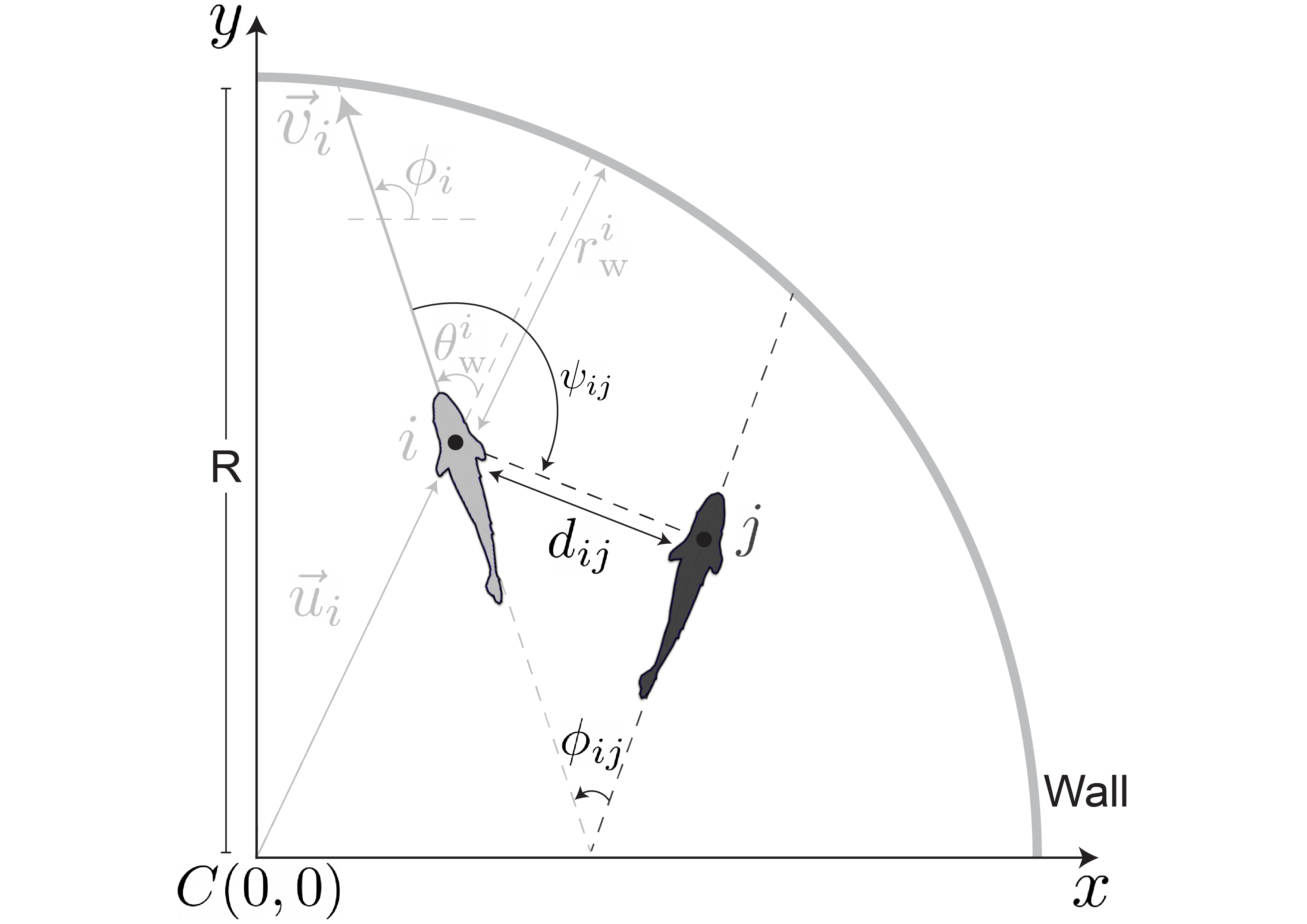
Figure 3: Individual and collective variables. For the focal agent $i$ (light gray) we define the individual quantities: $\vec{u}_{i}$ its Cartesian position, $\vec{v}_{i}$ its instantaneous velocity, $r_{\rm w}^{i}$ its distance to the wall, $\phi_{i}$ agent $i$’s heading angle. We also define the collective quantities from $i$’s perspective when its neighbor $j$ (dark gray) swims in the tank: interindividual distance $d_{ij}$. $R=25$ cm corresponds to the radius of the circular setup, $phi_{i}j$, the heading difference between both fish, and $\psi_{i}j$, the angle with which fish j is perceived by fish. Note that, for visualization purposes, the size of agents is not to scale.

II-C Evaluating the outcome of short- and long-term interactions between fish and the LureBot

Evaluating the extent to which models can reproduce the social dynamics of animal groups, here H. rhodostomus fish, is a non-trivial task. As explored in [36], such models may succeed in reproducing quantities in the short-term timescale, but may also fail to reproduce the emergent dynamics in the long term. Here, we opt to benchmark our results by exploiting the 9 observables considered in [36, 25] (see Fig. 3).

The first 3 observables correspond to instantaneous quantities at the individual level, for which we measure their probability density function (PDF): the speed, $V$ of an individual; its distance to the wall, $r_{\rm w}$; and its heading angle relative to the normal to the wall, $\theta_{\rm w}$. 3 additional observables probe the instantaneous collective dynamics: the distance $d_{ij}$ between the pair of individuals; the difference $|\phi_{ij}|$ between the heading directions of the two individuals ; and the angle $\psi_{ij}$ at which an individual perceives its neighbor. Finally, we consider 3 temporal correlation functions that probe the social dynamics at a very fine level [25], and which are generally particularly difficult to reproduce:

$$C_{X}(t) =\left\langle\left[\vec{u}_{i}(t+t^{\prime})-\vec{u}_{i}(t^{\prime})\right]^{2}\right\rangle,$$ (5)

$$C_{V}(t) =\left\langle\vec{v_{i}}(t+t^{\prime})\cdot\vec{v}_{i}(t^{\prime})\right\rangle,$$ (6)

$$C_{\theta_{\rm w}}(t) =\left\langle\cos\left[\theta_{\rm w}^{i}(t+t^{\prime})-\theta_{\rm w}^{i}(t^{\prime})\right]\right\rangle.$$ (7)

$C_{X}$ is the mean-squared displacement, $C_{V}$ the velocity autocorrelation, and $C_{\theta_{\rm w}}$ the autocorrelation of the angle of incidence to the wall. In general, we denote $C_{q}(t)=\langle q(t+t^{\prime})q(t^{\prime})\rangle$ as the average of the quantity $q(t)q(t+t^{\prime})$ over the reference times $t^{\prime}$, over individuals, and over different experiments. Assuming the stationarity of the system, the temporal correlation function $C_{q}(t)$ only depends on the time difference between observations, and is often noted $C_{q}(t)=\langle q(t)q(0)\rangle$ (implicitly implying an average over the reference time $t^{\prime}=0$).

III Dynamics of pairs of agents

In this work, we focus on the social dynamics that arise from pairwise interactions in three different conditions. First, we consider $\approx 11$ h of experiments involving pairs of H. rhodostomus, to characterize and quantify the spontaneous social interactions when no artificial devices are present in the tank.

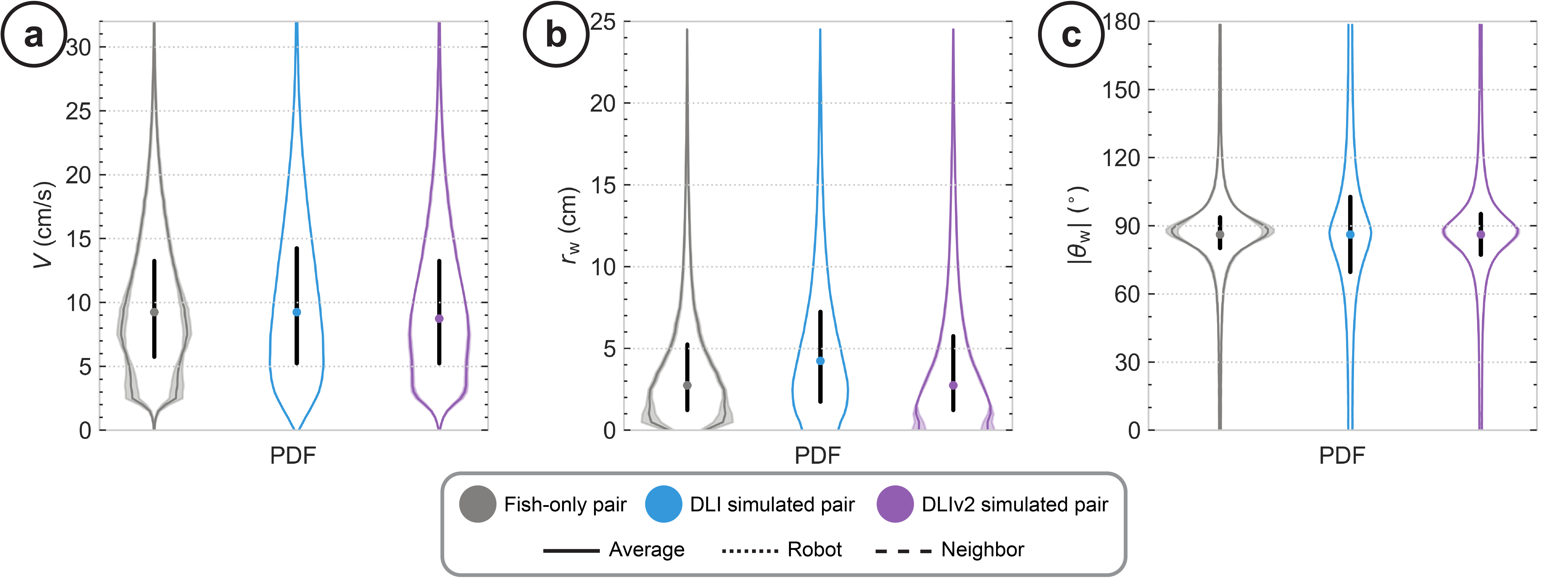
Figure S1: Instantaneous individual quantities. (a) Speed $V$ probability density function. (b) Distance to the wall $r_{\rm w}$ probability density function. (c) Angle of incidence to the wall $\theta_{\rm w}$ probability density function. Dark gray, blue, and red colors correspond to the distributions of the fish-only experiment, the DLI simulated pairs, and the DLIv2 simulated pairs, respectively. In all PDFs, the colored dot corresponds to the median, and the thick horizontal black line corresponds to the limits of the first and third quartile. The shaded areas correspond to the standard deviation.

Secondly, we consider $\approx 16$ h of effective trajectories for DLI simulated pairs (DLI-SP) [36], as a baseline to the robot’s underlying model in ideal conditions. This DLI model was originally trained in [36] on a different series of experimental data obtained in [11] for the same species (H. rhodostomus), but in different conditions (different tank but of same radius $R=25$ cm, lightning conditions…). We will also mention the results obtained after retraining the DLI model with the fish data considered in the present work, which we will refer to as the DLIv2-SP (see Supplementary Material and in particular Table S1 and Figs. S1-S3).

Finally, we conducted $\approx 11$ h of experiments where the LureBot propels a biomimetic lure moving inside the circular arena, which is interacting in closed-loop with an actual H. rhodostomus. For brevity, in the following analysis of the results, we will simply refer to the LureBot and the lure attached to it as the LureBot. The LureBot is given a pre-trained copy of the DLI model of [36], which is queried in real time to generate biomimetic trajectories (see Section II-B). We refer to these data as DLI biohybrid pairs (DLI-BP). We did not perform experiments with the LureBot trained with the DLIv2 model.

We explicitly designed a protocol which did not allow the use of the same fish in an experiment for at least $48$ h after their first test, to avoid potential learning effects when the fish interact with the lure. The fish housing conditions and experiments have been approved by the local ethical committee (see Section VI) and are described in detail in [35].

IV Results

This section reports the detailed comparison between the three test cases: 1) (fish-only) experiments with pairs of H. rhodostomus; 2) DLI simulated pairs (DLI-SP); and 3) DLI biohybrid pairs (DLI-BP), that consist of the LureBot interacting with a H. rhodostomus. In addition, at the end of this section, we will briefly present results for DLIv2 simulated pairs (DLIv2-SP).

The comparison between the different test cases exploits the observables described in Section II-C. For all quantities (PDF and correlation functions), we have computed the statistical and sample to sample standard error by using a bootstrap method. In addition, for each PDF, we report the mean and standard deviation (SD) in Table S1, as well as their standard error that we will omit to mention in the hereafter analysis of the results, for readability (except when their value is relevant to the discussion). Moreover, in order to compare the PDF for a given quantity between two given test cases, we compute the Hellinger distance between these distributions in Table S2. For two PDF $F$ and $G$ for the same quantity $x$, the Hellinger distance $H(F|G)$ quantifies their (dis)similarity [4, 5]:

$${H(F|G)} = \frac{1}{2}\int{{{\left({\sqrt{F(x)}-\sqrt{G(x)}}\right)}^{2}}}dx,$$ (8)

$$= 1-\int\sqrt{F(x)}\sqrt{G(x)}\,dx,$$

where we have used the normalization of the PDF, $\int F(x)\,dx=\int G(x)\,dx=1$, to obtain the last equality. The first definition of $H(F|G)$ clarifies that it measures the overall difference between $F(x)$ and $G(x)$. Meanwhile, the second equivalent definition provides a comprehensive interpretation in terms of the overlap of both PDF. Indeed, the second definition measures the distance from unity of the scalar product of $\sqrt{F(x)}$ and $\sqrt{G(x)}$ seen as vectors of unit Euclidean norm (a consequence of the normalization, $\int\sqrt{F(x)}^{2}\,dx=1$). The Hellinger distance is 0 if both PDFs are identical, and is bounded by 1, a limit reached if the distributions have a non-overlapping support. In general, a Hellinger distance $H(F|G)\lesssim 0.1$ points to a good agreement between both PDF, $0.1\lesssim H(F|G)\lesssim 0.2$ points to a fair similarity between them, while $H(F|G)\gtrsim 0.2$ indicates that the two distributions are significantly dissimilar.

IV-A Instantaneous individual observables

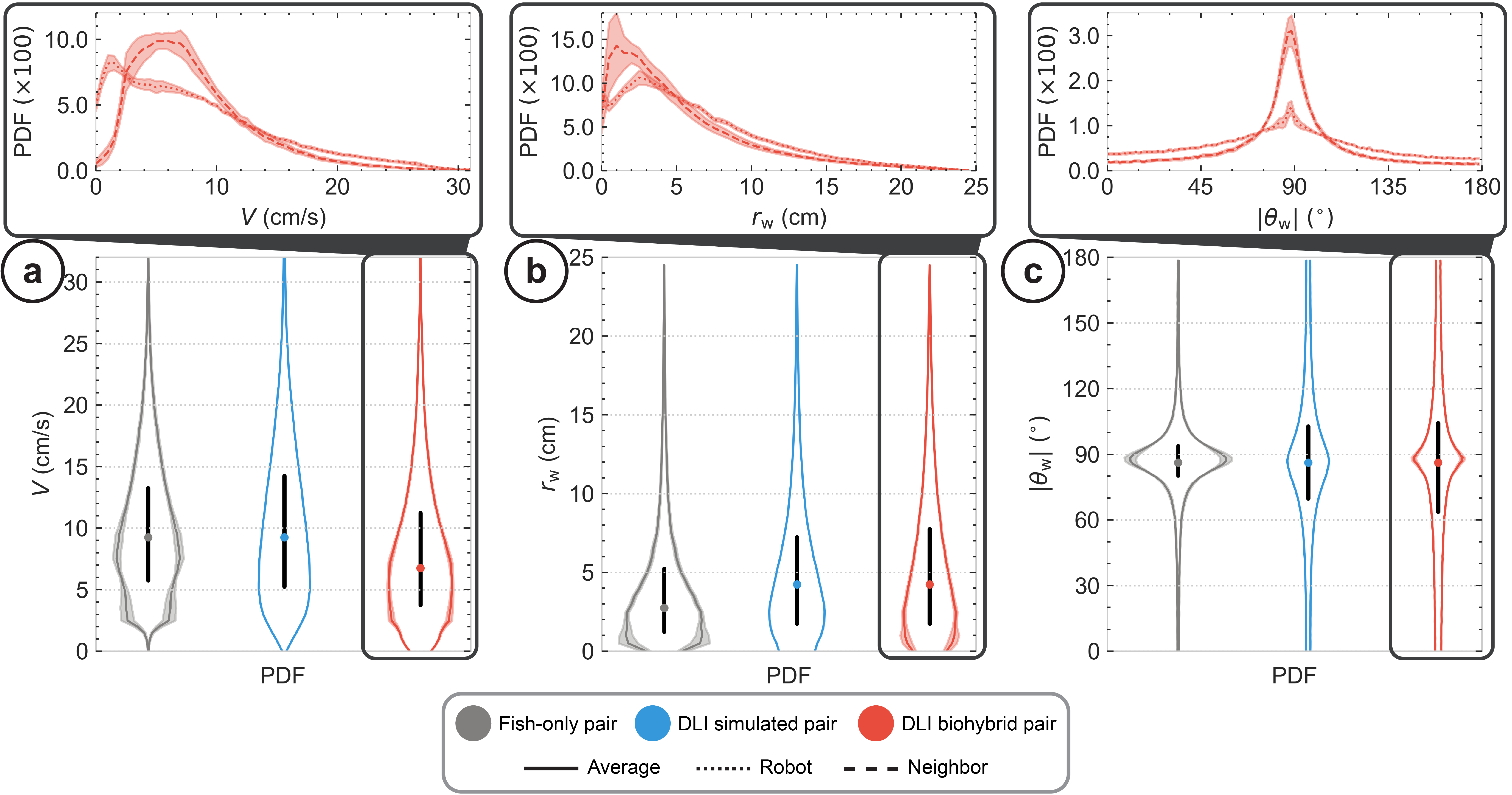
Figure 4: Instantaneous individual quantities. (a) Speed $V$ probability density function. (b) Distance to the wall $r_{\rm w}$ probability density function. (c) Angle of incidence to the wall $\theta_{\rm w}$ probability density function. Dark gray, blue, and red colors correspond to the distributions of the fish-only experiment, the DLI simulated pairs, and the DLI biohybrid pairs, respectively. In all PDFs, the colored dot corresponds to the median, and the thick horizontal black line corresponds to the limits of the first and third quartile. The inset plots depict the PDFs of the DLI biohybrid pair experiments where the dotted, dashed, and solid lines correspond to the robot, neighbor and average agent distributions, respectively. The shaded areas correspond to the standard deviation.

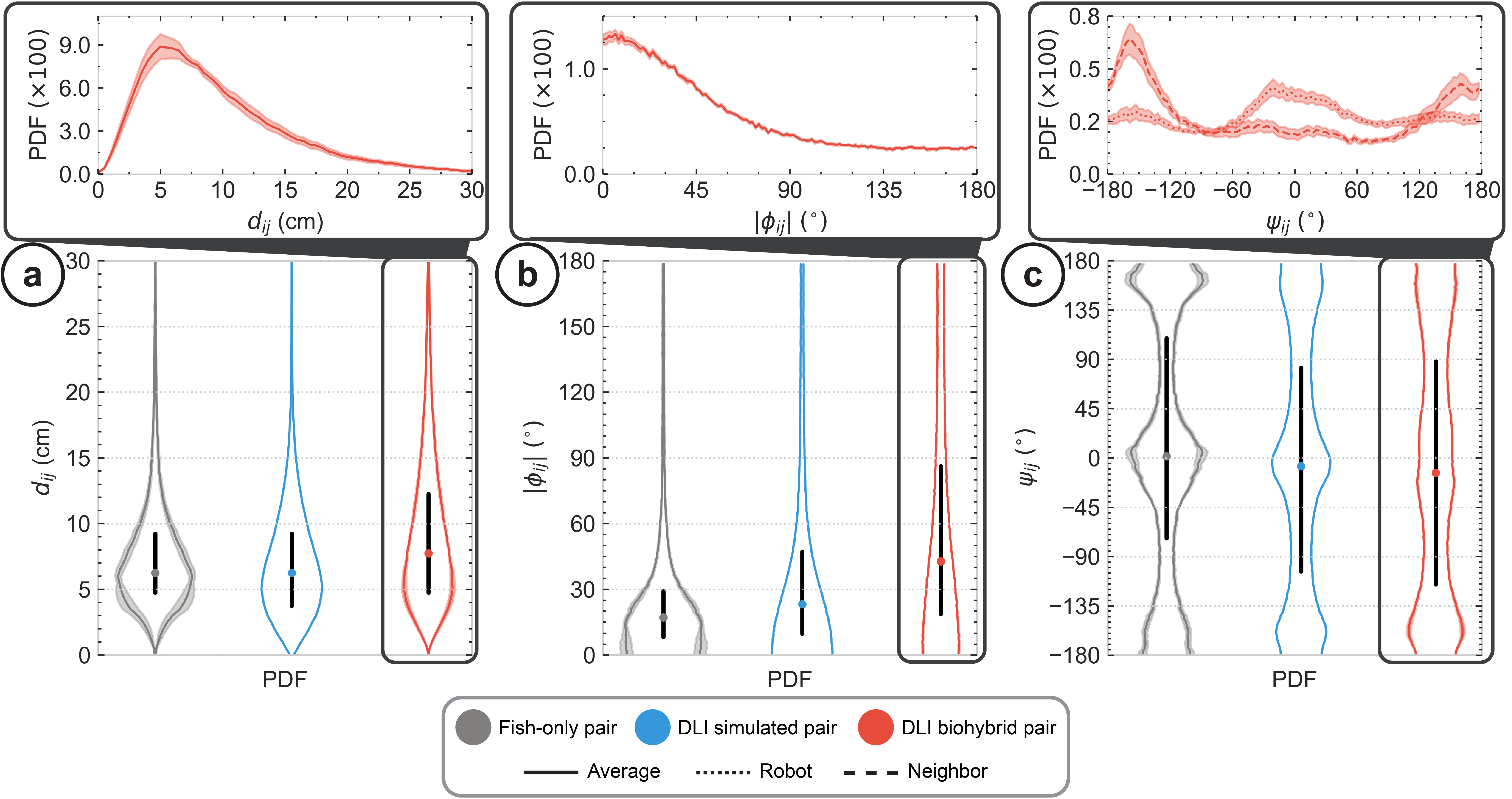
Figure 5: Instantaneous collective quantities. (a) Interindividual distance $d_{ij}$ probability density function. (b) Difference in heading angles $|\phi_{ij}|$ probability density function. (c) Viewing angle $\psi_{ij}$ probability density function. Dark gray, blue, and red colors correspond to the distributions of the experiment, DLI simulated pairs and DLI biohybrid pairs, respectively. In all PDFs, the colored dot corresponds to the median, and the thick horizontal black line corresponds to the limits of the first and third quartile. The inset plots depict the PDFs of the DLI biohybrid pair experiments where the dotted, dashed, and solid lines correspond to the robot, neighbor and average agent distributions, respectively. The shaded areas correspond to the standard deviation.

Fig. 4a shows the speed PDF for the three cases we considered. Fish pairs swim at a mean speed of $10.5$ cm/s, associated to a standard deviation (SD) of 5.7 cm/s (see Table S1). DLI simulated pairs produce a rather similar speed PDF (Hellinger distance $H=0.09$; see Table S2), albeit slightly wider (SD of 7.0 cm/s), with a nearly identical mean of 11.1 cm/s. For biohybrid pairs, the fish and the LureBot have a very similar mean speed (identical within error bars; see Table S1), but which is 20 % smaller than in the fish-only experiments, although the SD is similar to that of the fish experiments, resulting in a Hellinger distance of $H=0.18$.

In Fig. 4b, we plot the PDF of the distance to the wall, $r_{w}$, for each case. Fish pairs swim very close to the wall, with a mean distance of 4.4 cm and a SD of 3.9 cm, both comparable to the fish typical body length ($\sim$3.5 cm). This is a consequence of the burst-and-coast swimming mode exhibited by H. rhodostomus, as shown in [11]. Indeed, the motion of this species is characterized by a succession of sudden acceleration periods (“kicks” or bursts of typical duration 0.1 s), each followed by a longer gliding period of typical duration 0.5 s, during which the fish moves in a quasi straight line. Because of the rather narrow distribution of heading changes between kicks, even observed when a fish is far from the wall [11], the fish is unable to escape the concave boundaries of the wall, except when rare large heading changes occur. The mean distance to the wall is 5.7 cm for the DLI simulated pairs, and the associated PDF compared to that for fish experiments is $H=0.13$, showing that the DLI model captures reasonably well the tendency of the fish to move close to the wall. For biohybrid pairs, we found that the fish swims farther to the wall than in fish-only experiments, with a mean distance of 5.5 cm. In this case, the LureBot is even farther to the wall, at a mean distance of 6.6 cm, which likely also causes the fish to swim farther to the wall than in fish-only experiments.

Finally, in Fig. 4c, we plot the PDF of the absolute value of the heading angle relative to the normal to the wall, $|\theta_{\rm w}|$. As a consequence of the agents (fish, DLI model, or LureBot) moving close to the wall, we naturally find that the mean of $|\theta_{\rm w}|$ is very close to, but slightly below 90^∘ (see Table S1), a difference which is statistically significant. Indeed, as already reported in the experiments of [11], the agents spend slightly more time heading toward the wall ($|\theta_{\rm w}|<90^{\circ}$) than moving away from it ($|\theta_{\rm w}|>90^{\circ}$). The PDF for the three considered cases are symmetric around their mean, but we find that the fish experiments lead to the narrowest distribution, with a SD of 22^∘, compared to a SD of 35^∘ for the DLI simulated pairs, and a SD of 33^∘ and 43^∘ for the fish and the LureBot in a biohybrid pair. The values of these SD are naturally correlated with the mean distance of the agent to the wall: the farther the agent, the larger are the fluctuations (SD) of its heading angle relative to the wall. Note that although the SD is larger for biohybrid pairs than for DLI simulated pairs (and for fish pairs), the intensity of the peak near $|\theta_{\rm w}|=90^{\circ}$ is larger for biohybrid pairs, which will have further consequences when we will address the temporal correlations of $\theta_{\rm w}$ (see Section IV-C).

In summary, DLI-BP achieve fair agreement with the experimental results for all quantities. Concurrently, DLI-BP and DLI-SP show smaller dissimilarity, indicating that the transposition of the simulated model into the robot was successful leading a good overall precision (see Table S2). We also observe that, in some cases (e.g., $|\theta_{\rm w}|$), the fish’s behavior guides the DLI-powered robot to approximate the experimental dynamics better, either due to unaccounted for dynamics in the model or due to an adapted fish behavior caused by the robot’s presence. Nonetheless, the observables test the DLI’s performance at a very fine level, especially in the case of DLI-BP, where the physical aspect is also impeding the precise reproduction of the social dynamics, either due to the imperfect (with respect to fish) motion of the robot or the varying degree the robotic system’s acceptance by the fish.

IV-B Instantaneous collective observables

H. rhodostomus have a natural tendency to swim in close proximity to each other. In our experiments, fish pairs typically maintain a median interindividual distance $d_{ij}$ of less than two body lengths (see Fig. 5a), with a mean distance of $8.05\pm 0.71$ cm and a SD of 5.1 cm (see Table S1). The dynamics of DLI simulated pairs results in a very similar PDF ($H=0.16$), with a mean of $7.43\pm 0.03$ cm, which is within one standard error (for the fish experiments) from the mean obtained for fish. As for the biohybrid pair, it is less bound than pairs of fish or DLI, with a mean distance between the fish and the LureBot of $9.96\pm 0.48$ cm. The distribution is also slightly wider, with a SD of 6.3 cm. In fact, although the peak of the interindividual distance PDF is located at a similar value as for fish or DLI pairs ($5-6$ cm in the three cases), the biohybrid pairs are more often separated by a distance larger than 15 cm.

H. rhodostomus is a social species, often found to form well aligned schools. In fact, their pairwise alignment interaction was quantitatively measured in [11], showing that this interaction remains strong up to three body lengths, well within the typical distance between fish. In Fig. 5b, to quantify the alignment within pairs of agents, we plot the distribution of the absolute value of the difference between the heading angles of the two agents, $|\phi_{ij}|$ (see the graphical definition in Fig. 3). The mean heading difference observed in fish experiments is 27^∘, with a rather narrow PDF associated with a SD of 30^∘, confirming the good level of alignment between the two fish. The DLI simulated pairs are not as aligned as fish pairs, with a larger mean and SD equal to 38^∘, although the Hellinger distance between the two PDF $(H=0.14)$ remains satisfactory. The corresponding PDF for biohybrid pairs exhibits the largest disagreement with the fish experiments of all the PDF presented here ($H=0.30$). Indeed, despite also being peaked at $|\phi_{ij}|=0$, the PDF has a non-negligible weight for $|\phi_{ij}|>90^{\circ}$, resulting in a much larger mean of $59^{\circ}$ and a SD of $48^{\circ}$. This wider PDF is a consequence of the fact that the fish and the LureBot, despite remaining close to each other on average, have a much higher probability than fish pairs to be at a distance above the range of the alignment interaction. Moreover, when the fish and the LureBot are far apart and attempt to get closer, they have a high chance to be actually anti-aligned during this process, hence the significant weight of the PDF near $|\phi_{ij}|=180^{\circ}$.

Finally, Fig. 5c shows the PDF of the angle of perception $\psi_{ij}$, defined in Fig. 3. For pairs of fish, the PDF presents clear peaks at $\psi_{ij}=0^{\circ}$ and near $|\psi_{ij}|=180^{\circ}$. This indicates that the well aligned fish are following each other rather than swimming side by side. For DLI simulated pairs, the same pattern is observed but with slightly less pronounced peaks, although the Hellinger distance of $H=0.05$ confirms the excellent agreement between both PDF. As for the biohybrid pair, the PDF averaged over the fish and the LureBot again presents the same peaks as before, but even less pronounced. Again, the less sharp peaks are a consequence of the fact that the biohybrid pairs stand farther from the wall than fish pairs, and above all, of the fact that their distance has a higher probability to be large enough so that their angle of perception $\psi_{ij}$ becomes uncorrelated. The lesser alignment of the biohybrid pairs (see above) originates from the same causes, and in turn also results in a more homogeneous distribution of the angle of perception. However, the apparent reasonable agreement with the PDF for the fish-only and DLI-SP pairs masks the difference between the PDF for the fish and for the LureBot shown in the top inset of Fig. 5c. There, we observe that the peak near $\psi_{ij}=0^{\circ}$ is dominated by the contribution of the fish, showing that the fish more often follows the LureBot than the converse. In addition, we find that the PDF for the fish is also peaked slightly above $\psi_{ij}=-180^{\circ}$, while the PDF for the LureBot has a corresponding peak slightly below $\psi_{ij}=+180^{\circ}$. By periodicity of 360^∘, these two peaks are obviously located at almost the same angle, but this slight angular shift translates to the fact that the fish is, on average, slightly closer to the wall than the LureBot, as noted in Section IV-A.

The instantaneous collective quantities demonstrate that despite the dissimilarities measured in the individual behavior of both DLI-SP and DLI-BP with respect to the fish-only experiment, the collective dynamics are fairly reproduced. Furthermore, the DLI is transferred in a physical system with good agreement compared to its simulated version, and the living agent responds positively. However, the angular control of the robot is arguably less precise, which contributes to the general deviation from the experimental angle-related distributions.

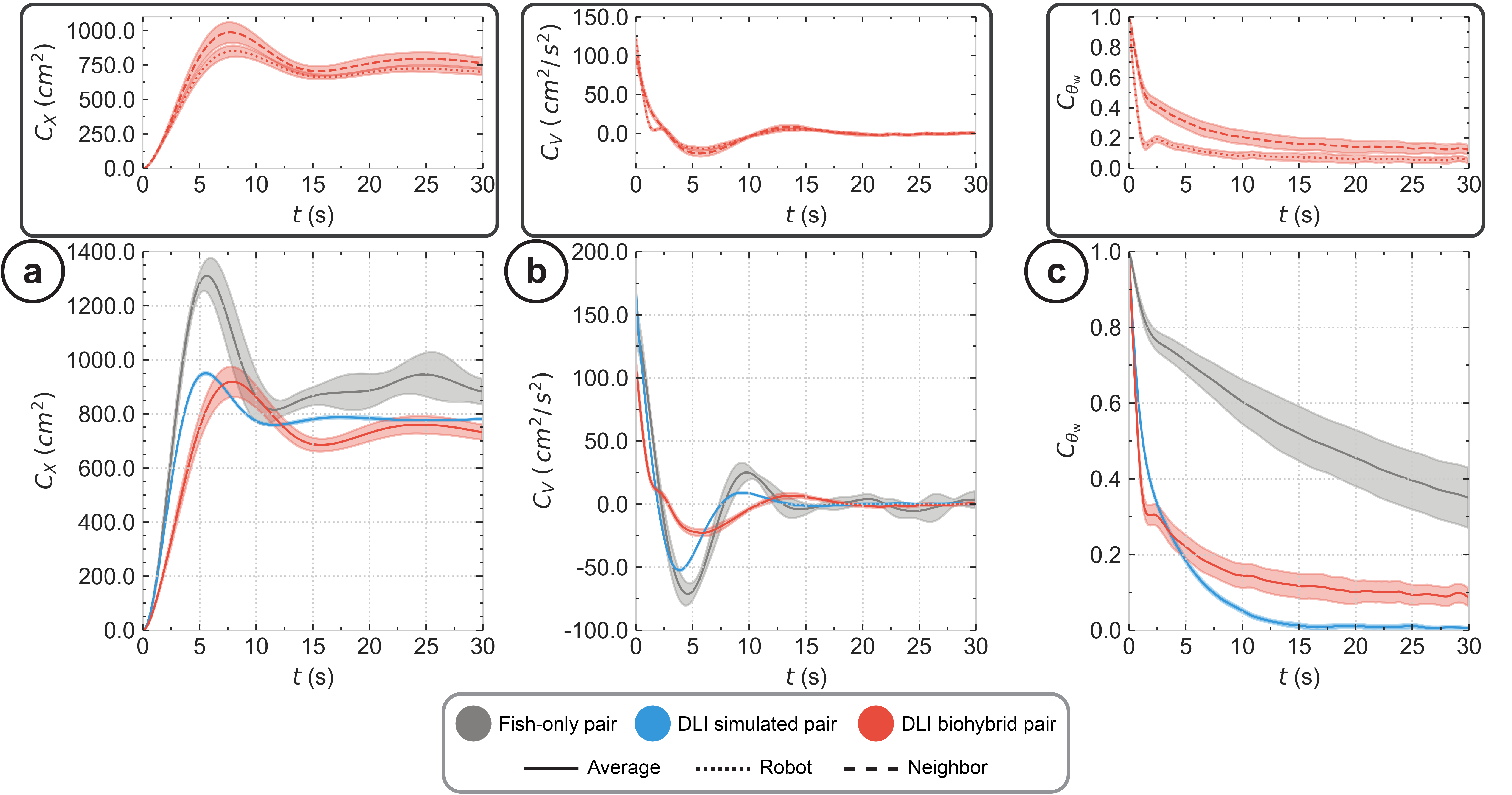
Figure 6: Temporal correlation quantities. (a) Mean squared displacement $C_{X}(t)$. (b) Velocity autocorrelation $C_{V}(t)$. (c) Temporal correlations of the angle of incidence to the wall $C_{\theta_{\rm w}}(t)$. Dark gray, blue and red colors correspond to the distributions of the experiment, DLI simulated pairs and DLI biohybrid pairs, respectively. Dotted, dashed and solid lines indicate the robot, neighbor and average agent distributions, respectively. The shaded areas correspond to the standard deviation.

IV-C Temporal correlation functions

In Fig. 6, we plot the three observables used to quantify the temporal correlations that emerge in the system during the long-term dynamics, which are defined in Section II-C.

Fig. 6a shows the mean square displacement of the agents, $C_{X}(t)$, in the three considered cases. After a rapid growth, $C_{X}(t)$ presents a peak and an ultimate decay to a mean level equal to twice the mean square of the distance to the center of the tank. Indeed, for large time difference, the positions at time $t^{\prime}$ and $t+t^{\prime}$ become uncorrelated, and we obtain

$$C_{X}(t) = \left\langle\left[\vec{u}_{i}(t+t^{\prime})-\vec{u}_{i}(t^{\prime})\right]^{2}\right\rangle$$ (9)

$$\mathop{\approx}\limits_{t\to+\infty} \left\langle\vec{u}_{i}^{2}(t+t^{\prime})\right\rangle+\left\langle\vec{u}_{i}^{2}(t^{\prime})\right\rangle$$

$$= 2\left\langle\vec{u}_{i}^{2}(t^{\prime})\right\rangle,$$

which becomes time-independent due to the stationarity of the dynamics. Although $C_{X}(t)$ has the same qualitative form in the three cases, one observes differences in the position and height of the peak and in the asymptotic value. The latter is explained by the fact that the closer the agents are to the wall, the larger is the mean square of their distance to the center of the tank, $\left\langle\vec{u}_{i}^{2}(t^{\prime})\right\rangle$. Indeed, we have found, in Section IV-A, that fish pairs swim closest to the wall, while biohybrid pairs are the farthest, which is consistent with the asymptotic behavior of $C_{X}(t)$ observed in Fig. 6a. Furthermore, the top inset of Fig. 6a for the biohybrid pairs shows that $C_{X}(t)$ for the fish is systematically larger than for the LureBot, which is also consistent with the fact that the fish swims slightly closer to the wall than the LureBot. As for the position of the peaks in Fig. 6a, it roughly corresponds to the time for the corresponding agent to travel half of the tank perimeter. This time is directly correlated with the mean speed of the agent. In Section IV-A, we found that the fish pairs and DLI simulated pairs had essentially the same mean speed, which explains the agreement between the position of the corresponding peaks in $C_{X}(t)$. However, we also found that the biohybrid pairs were $20$ % slower, which explains the fact that the peak in their $C_{X}(t)$ is reached at a later time than for fish and DLI pairs.

Fig. 6b shows the velocity autocorrelation, $C_{V}(t)$, in the three considered cases, which vanishes for $t$ large enough, when the velocity at time $t+t^{\prime}$ becomes uncorrelated with that at time $t^{\prime}$. It can be formally shown that $C_{V}(t)=d^{2}C_{X}(t)/dt^{2}$ (although this relation is only approximate, when the 2 quantities are observed independently over a finite sampling time), so that the interpretation of the shape of $C_{V}(t)$ results from the analysis that we have presented above for $C_{X}(t)$. In particular, the peaks of the first two oscillations in $C_{V}(t)$ roughly correspond to the two inflection points just before and after the main peak in $C_{X}(t)$. In addition, $C_{V}(t=0)$ is the mean square velocity, and we indeed observe an agreement between its value for fish and DLI pairs, while the slower biohybrid pairs result in a lower initial value of $C_{V}(t=0)$ in this case.

Finally, the (most subtle) temporal correlation function of the heading of an agent relative to the wall, $C_{\theta_{\rm w}}(t)=\left\langle\cos\left[\theta_{\rm w}^{i}(t+t^{\prime})-\theta_{\rm w}^{i}(t^{\prime})\right]\right\rangle$, is shown in Fig. 6c. For very large time $t$, $C_{\theta_{\rm w}}(t)$ must obviously decay, but we observe that for fish pairs, we still have $C_{\theta_{\rm w}}(t=30\,{\rm s})\approx 0.35$, indicating strong correlations. For DLI simulated pairs, We find that $C_{\theta_{\rm w}}(t)$ vanishes very rapidly ($C_{\theta_{\rm w}}(t=15\,{\rm s})\approx 0$). Finally, for biohybrid pairs, we still observe some weak remnant correlations at $t=30\,{\rm s}$, with $C_{\theta_{\rm w}}(t=30\,{\rm s})\approx 0.1$ (although the correlation is dominated by the contribution of the fish, as shown in the top inset of Fig. 6c). Here, the decay rate of $C_{\theta_{\rm w}}(t)$ is strongly related to the sharpness of the peak near $\theta_{\rm w}=90^{\circ}$ in the PDF of $\theta_{\rm w}$ (see Fig. 4c and Section IV-A). Indeed, a sharp peak suggests that it can take a long time to explore values of $\theta_{\rm w}$ far from $90^{\circ}$, leading to a slower decay of $C_{\theta_{\rm w}}(t)$. Accordingly, we indeed found that the least sharp peak in the PDF of $\theta_{\rm w}$ is observed for DLI simulated pairs, resulting in the fastest decay of $C_{\theta_{\rm w}}(t)$ in this case.

Both the DLI-SP and DLI-BP fail to precisely reproduce the correlation function $C_{\theta_{\rm w}}(t)$, producing a very similar sharp decay compared to the one of real fish. This is derived by the DLI’s tendency to frequently produce trajectories farther from the wall than what observed in the experiment. Despite an overall dissimilarity between the experiment and the DLI derivatives, the DLI-BP remains fairly faithful to the DLI-SP. Yet again, this indicates that the DLI is missing some aspects of the social dynamics before being implemented on the robot, but the robot performs reasonably well in reproducing its underlying model.

IV-D Complementary results for DLIv2 simulated pairs

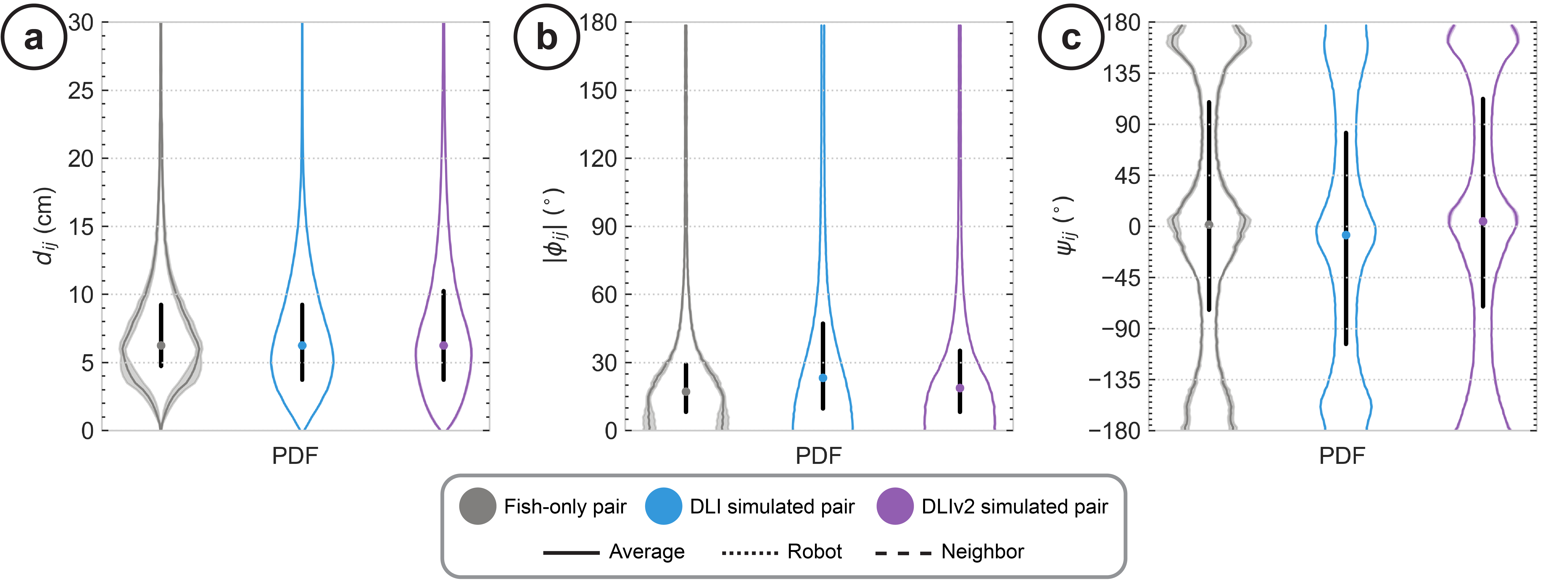
Figure S2: Instantaneous collective quantities. (a) Interindividual distance $d_{ij}$ probability density function. (b) Difference in heading angles $|\phi_{ij}|$ probability density function. (c) Viewing angle $\psi_{ij}$ probability density function. Dark gray, blue, and red colors correspond to the distributions of the experiment, DLI simulated pairs and DLIv2 simulated pairs, respectively. In all PDFs, the colored dot corresponds to the median, and the thick horizontal black line corresponds to the limits of the first and third quartile. The shaded areas correspond to the standard deviation.

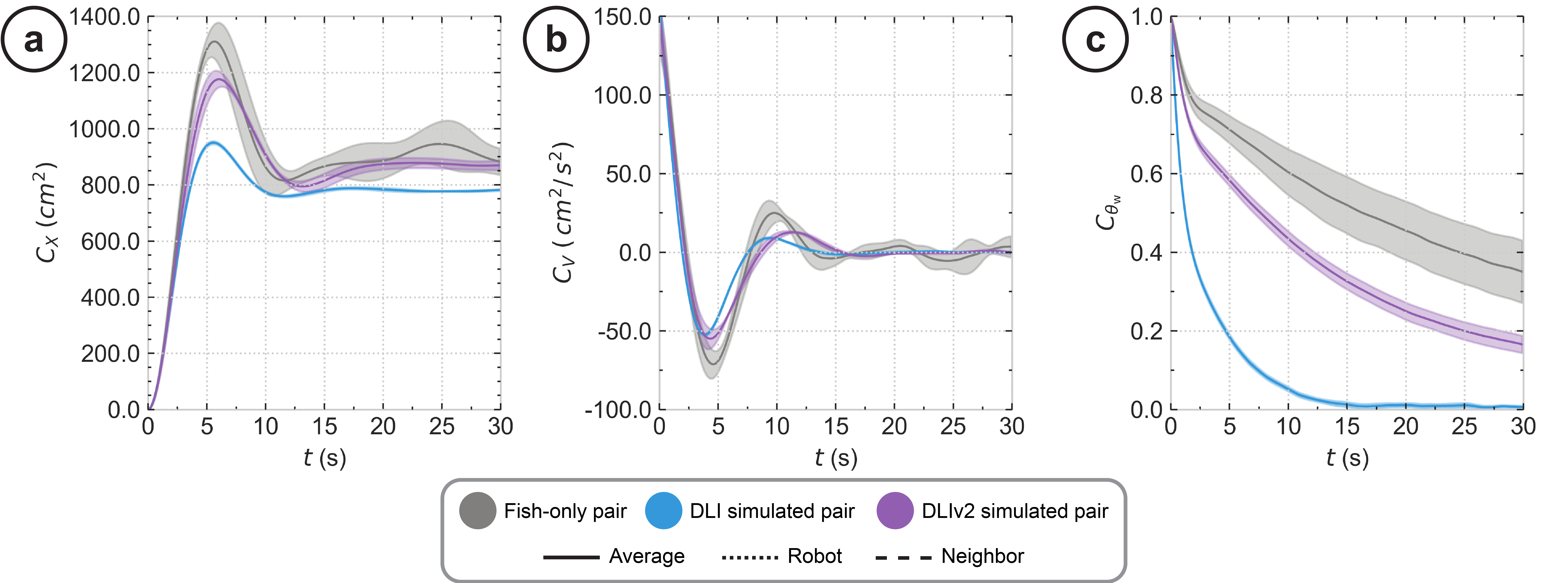
Figure S3: Temporal correlation quantities. (a) Mean squared displacement $C_{X}(t)$. (b) Velocity autocorrelation $C_{V}(t)$. (c) Temporal correlations of the angle of incidence to the wall $C_{\theta_{\rm w}}(t)$. Dark gray, blue and red colors correspond to the distributions of the experiment, DLI simulated pairs and DLIv2 simulated pairs, respectively. The shaded areas correspond to the standard deviation.

In addition to the Deep Learning Interaction (DLI) pretrained network utilized in the previous sections, we have also considered an updated version, the DLIv2. This version was retrained on data gathered from the present fish-only experiments under new lighting conditions, concurrently to the robot experiments presented in this work, so that retraining was only feasible after their completion. However, it provided us with the opportunity to test the scalability and predictive performance of the pretrained DLI with new input samples, which, while not fundamentally different, originated from altered social dynamics. For this purpose, we conducted extensive simulations with the DLIv2, and found that their results are in excellent agreement with the present fish-only pair experiments (see Tables S1 and S2 for further details) for the individual (see Fig. S1) and collective (see Fig. S2) observables, and for the temporal correlation functions (see Fig. S3). The performance of the simulated DLIv2 model present a significant improvement compared to that of the pretrained DLI model, and one could expect that the LureBot commanded by the DLIv2 model would lead to better results than for the LureBot commanded by the pretrained DLI model. Yet, our point here is that the pretrained DLI model, in different experimental conditions, can still interact with a fish in a similar way as a fish would do.

V Discussion and Conclusion

Despite the abundance of studies on fish-robot interactions, to our knowledge, no prior research has drawn comparisons between the social interaction dynamics produced by fish-only, biohybrid, and simulated groups. This comparison also introduces an intriguing issue: while the reality gap in robotics [32] typically pertains to the transferability of robot controllers from simulation to real-life conditions, a parallel can be drawn for biohybrid social interactions, termed the biomimicry gap. Addressing this gap is complicated by: 1) subtle behavioral patterns that researchers or machines fail to consider during the modelling process, 2) the inherently imperfect biomimetic properties of artificial lures and devices, and 3) the absence of physics in most models. Constructing biohybrid systems with minimal or, ideally, no biomimicry gap, thus making them indistinguishable from pure animal groups, could open doors to groundbreaking research in biological systems. This would enable, for example, the introduction of controlled, localized perturbations to accurately gauge an animal’s reaction. Such endeavors require that any non-biomimetic effects of the robot be stringently assessed and alleviated. It is therefore crucial to ensure that models do not simply overfit experimental data, but genuinely translate to real-world scenarios, through robotic systems that can reproduce these models as expected.

Alas, while substantial progress has been made in the intersection of behavioral modeling and robotics hardware which has long been promoted as the key to unraveling and understanding the mechanisms that underlie collective behavior in animal groups, this assertion has not been convincingly demonstrated in the literature. Especially in terms of models, most biohybrid systems are designed to modulate collective decisions between a limited set of spatial choices (which often resolves to a binary choice). Many of these systems rely on simplified passive (open-loop) [37, 38, 1, 28, 46, 45, 3, 27, 10] or reactive (closed-loop) [17, 13, 21, 47, 30, 29, 40, 26] models, with only a handful utilizing biomimetic models. Even fewer biomimetic models have been successfully tested in biohybrid groups [17, 13] to emulate real-life dynamics of fish groups. Simultaneously, to our knowledge, no end-to-end machine learning (ML) model has been examined in this context, despite the booming field of ML. Assessing a model’s fidelity is particularly challenging in the case of ML models, which are often black-box (i.e., not easily explainable). Moreover, our understanding of how well robotic devices can integrate and interact with living animal groups primarily relies on metrics that do not account for model limitations. Similarly, many models evaluated in simulations, rely on metrics that do not account for how such models can scale to real life [12, 15, 13]. Finally, the role of biomimetic lures and agile robotic devices in such studies is usually underplayed. That is, there is insufficient evidence to support the claim that biomimetic systems can bridge the biomimicry gap.

In this work, through the precise and comparative quantification of collective behavior in pairs of agents (fish-only pairs, DLI simulated pairs and DLI biohybrid pairs), we demonstrate that our biomimetic lure and robot system [35], combined with the DLI, are capable of bridging a substantial part of the biomimicry gap. More specifically, our study reveals that the overall gap between actual pairs of H. rhodostomus and simulation is smaller (root mean squared Hellinger distance of 0.12 of all observables) than that of the simulation and the biohybrid experiment (root mean squared Hellinger distance of 0.14 of all observables), or the biohybrid pairs compared to fish-only pairs (root mean squared Hellinger distance of 0.20 of all observables). In essence, our DLI model is successful in generating realistic social interactions [36], our robotic system is very capable of replicating its instructions with small discrepancies, but the transferred model results in greater discrepancies and the gap widens compared to the simulation (see Table S2). Nonetheless, the biohybrid pair is not well aligned compared to fish groups, which is confirmed when we compute the largest Hellinger distance value out of the quantities considered (Hellinger distance between angle of incidence PDF is $H=0.30$), and is the largest contributor to widening the social interaction discrepancies (i.e., the largest contributor, out of all observables, to increasing the Hellinger distance). These discrepancies are consequently observed for the correlation function of the angle of incidence to the wall. It is worth noting that even in fish-only experiment comparisons, the Hellinger distance will probably exceed zero (albeit it is expected to be close to it), owing to the inherent behavioral variability fish display between experiments. This suggests that the primary goal for robotic systems might be to significantly reduce the gap, rather than entirely eliminating it.

Therefore, despite the positive results highlighted in our study, we demonstrated that further closing the biomimicry gap requires work on minimizing all three discrepancy sources (depicted in Fig. 1). First, it requires that we refine our modelling approaches (e.g., by repeating the experiments with the DLIv2). Second, the physics-related discrepancies, primarily attributable to the transposition of the model into the robot, remains relatively small, but also requires measurable improvement in the robotic system’s operation to fully bridge the gap. Finally, discrepancies in the communication cues pose a considerable challenge in terms of evaluation and could only be fully measured in the absence of the other two sources of discrepancies. These discrepancies might correlate with the way social interactions are faithfully modeled, under the assumption that the real fish’s responses change due to the artificial lure, potentially influencing the interaction dynamics it is exhibiting in unexpected ways (i.e., not frequently or at all observed in spontaneous interactions). Whereas it remains indeterminate as to what constitutes the ultimate goal in reducing the biomimicry gap, our study introduces a methodology and the resulting baseline values that produced realistic interactions. Furthermore, the correlation between improving the Hellinger distance and reducing the gap is not yet known, but future studies can leverage the values presented in this study as a baseline comparison score. To that end, along with the between-sample noise that we measured with our bootstrap approach, future work could include independently repeating the entirety of the fish-only experiments to provide insight into the behavioral variability of H. rhodostomus. In turn, this could provide better understanding into a sensible lower bound for the average Hellinger distance value, that indicates excellent agreement between any two datasets.

We believe our study may be the first of many that emphasizes on both simulated and biomimetic biohybrid experiments in a single end-to-end approach. An approach that, as demonstrated, allows us to gain more insight into which aspects led to behavioral differences in the biohybrid experiments and, therefore, need improvement. In turn, this contributes to: 1) establishing a better experimentation pipeline to investigate the varying sources of gaps (e.g., physical robot limitations, social interaction gaps in models, and eventually discrepancies in the communication cues exploited to evoke responses), and 2) drawing more definitive and insightful behavioral conclusions without the unrealistic effects introduced by the robotic system and social interaction models. In future work, we aim to test the DLI with multiple neighbors and species, thereby gaining further insight into how our model scales to multiagent interactions and whether large groups of living animals are equally receptive to the DLI-driven artificial agent. We also aim to consistently report the biomimicry gap score (in the form of the quantities presented), in the hope that future studies may standardize and utilize a common methodology to evaluate the fidelity of biohybrid systems with respect to natural ones.

VI Ethics statement

Experiments were approved by the local ethical committee for experimental animals and were performed at the Centre de Recherches sur la Cognition Animale, Centre de Biologie Intégrative, Toulouse, in an approved fish facility (A3155501) under permit APAFIS$\#$27303-2020090219529069 v8 in agreement with the French legislation.

Supplementary Material

Supplementary Video S1

Video segments for fish-only experiments, DLI simulated pairs (DLI-SP), and biohybrid pairs (DLI-SP). https://doi.org/10.5281/zenodo.8253256

Supplementary Tables

TABLE S1: Means and standard deviations. For the case of fish-only experiments, DLI simulated pairs (DLI-SP), and biohybrid pairs (DLI-SP), we report the mean and the standard deviation (SD) of the 6 observables introduced in Section II-C, along with their respective standard error. The speed $V$ is given in cm/s, the distances $r_{\textrm{w}}$ and $d_{ij}$ are given in cm, and the angles $|\theta_{\textrm{w}}|$, $|\phi_{ij}|$, and $\psi_{ij}$ are in degrees. Note the small standard error in the case of the (DLI-SP) resulting from extensive simulations (16.6 h long, almost twice the amount of data collected for other cases) and the fact that the 2 agents are statistically identical. For the biohybrid experiments, we report the mean and SD for $V$, $r_{\textrm{w}}$, and $|\theta_{\textrm{w}}|$, averaged over the fish and the LureBot, as well as for each of them. Finally, we present the corresponding results for a DLI model retrained on the present fish experiments (DLIv2-SP).

Pair	Quantity	Mean	Standard deviation
Fish-only	$V$	$10.50\pm 0.60$	$5.73\pm 0.36$
	$r_{\textrm{w}}$	$4.39\pm 0.43$	$3.86\pm 0.22$
	$|\theta_{\textrm{w}}|$	$87.42\pm 0.39$	$21.91\pm 1.46$
	$d_{ij}$	$8.05\pm 0.71$	$5.11\pm 0.43$
	$|\phi_{ij}|$	$26.72\pm 1.91$	$29.81\pm 1.24$
	$\psi_{ij}$	$7.96\pm 4.73$	$108.98\pm 1.19$
DLI-SP	$V$	$11.06\pm 0.04$	$7.04\pm 0.02$
	$r_{\textrm{w}}$	$5.66\pm 0.03$	$4.42\pm 0.03$
	$|\theta_{\textrm{w}}|$	$88.07\pm 0.06$	$34.55\pm 0.16$
	$d_{ij}$	$7.43\pm 0.03$	$4.38\pm 0.04$
	$|\phi_{ij}|$	$38.06\pm 0.19$	$38.63\pm 0.17$
	$\psi_{ij}$	$-4.11\pm 0.33$	$107.13\pm 0.06$
DLI-BP	$V$	$8.60\pm 0.22$	$5.93\pm 0.12$
	$r_{\textrm{w}}$	$6.05\pm 0.25$	$4.76\pm 0.06$
	$|\theta_{\textrm{w}}|$	$86.44\pm 0.17$	$38.07\pm 0.73$
	$d_{ij}$	$9.96\pm 0.48$	$6.27\pm 0.33$
	$|\phi_{ij}|$	$58.60\pm 0.91$	$48.38\pm 0.24$
	$\psi_{ij}$	$-7.42\pm 4.16$	$110.41\pm 0.51$
DLI-BP (fish)	$V$	$8.44\pm 0.26$	$5.13\pm 0.21$
	$r_{\textrm{w}}$	$5.54\pm 0.35$	$4.54\pm 0.09$
	$|\theta_{\textrm{w}}|$	$87.46\pm 0.19$	$32.76\pm 1.25$
DLI-BP (robot)	$V$	$8.74\pm 0.16$	$6.62\pm 0.12$
	$r_{\textrm{w}}$	$6.59\pm 0.15$	$4.91\pm 0.05$
	$|\theta_{\textrm{w}}|$	$85.42\pm 0.24$	$42.78\pm 0.79$
DLIv2-SP	$V$	$10.53\pm 0.48$	$6.18\pm 0.28$
	$r_{\textrm{w}}$	$4.64\pm 0.23$	$4.37\pm 0.05$
	$|\theta_{\textrm{w}}|$	$87.56\pm 0.11$	$26.47\pm 0.47$
	$d_{ij}$	$8.39\pm 0.07$	$6.15\pm 0.11$
	$|\phi_{ij}|$	$30.54\pm 0.30$	$33.11\pm 0.29$
	$\psi_{ij}$	$11.72\pm 0.87$	$109.08\pm 0.19$

TABLE S2: Hellinger distances. We exploit the Hellinger distance between two PDF to compare the PDF of the 6 observables introduced in Section II-C, for fish-only experiments, DLI simulated pairs (DLI-SP), and biohybrid pairs (DLI-SP).

Pair	Quantity	Hellinger distance
Fish-only vs DLI-SP	$V$	$0.09$
	$r_{\textrm{w}}$	$0.13$
	$|\theta_{\textrm{w}}|$	$0.23$
	$d_{ij}$	$0.12$
	$|\phi_{ij}|$	$0.14$
	$\psi_{ij}$	$0.09$
Fish-only vs DLI-BP	$V$	$0.18$
	$r_{\textrm{w}}$	$0.15$
	$|\theta_{\textrm{w}}|$	$0.25$
	$d_{ij}$	$0.16$
	$|\phi_{ij}|$	$0.30$
	$\psi_{ij}$	$0.15$
DLI-SP vs DLI-BP	$V$	$0.14$
	$r_{\textrm{w}}$	$0.04$
	$|\theta_{\textrm{w}}|$	$0.04$
	$d_{ij}$	$0.18$
	$|\phi_{ij}|$	$0.17$
	$\psi_{ij}$	$0.07$
Fish-only vs DLIv2-SP	$V$	$0.05$
	$r_{\textrm{w}}$	$0.08$
	$|\theta_{\textrm{w}}|$	$0.08$
	$d_{ij}$	$0.14$
	$|\phi_{ij}|$	$0.06$
	$\psi_{ij}$	$0.04$

Supplementary Figures

References

- [1] Nicole Abaid, Tiziana Bartolini, Simone Macrì, and Maurizio Porfiri, Zebrafish responds differentially to a robotic fish of varying aspect ratio, tail beat frequency, noise, and color, Behavioural brain research 233 (2012), no. 2, 545–553.
- [2] Nicole Abaid and Maurizio Porfiri, Fish in a ring: spatio-temporal pattern formation in one-dimensional animal groups, Journal of The Royal Society Interface 7 (2010), no. 51, 1441–1453.
- [3] Tiziana Bartolini, Violet Mwaffo, Ashleigh Showler, Simone Macrì, Sachit Butail, and Maurizio Porfiri, Zebrafish response to 3d printed shoals of conspecifics: the effect of body size, Bioinspiration & biomimetics 11 (2016), no. 2, 026003.
- [4] Ayanendranath Basu, Ian R Harris, and Srabashi Basu, 2 minimum distance estimation: The approach using density-based distances, Handbook of Statistics 15 (1997), 21–48.
- [5] Rudolf Beran, Minimum hellinger distance estimates for parametric models, The annals of Statistics (1977), 445–463.
- [6] Frank Bonnet, Stefan Binder, Marcelo Elias de Oliveria, José Halloy, and Francesco Mondada, A miniature mobile robot developed to be socially integrated with species of small fish, 2014 IEEE International Conference on Robotics and Biomimetics (ROBIO 2014), IEEE, 2014, pp. 747–752.
- [7] Frank Bonnet, Alexey Gribovskiy, José Halloy, and Francesco Mondada, Closed-loop interactions between a shoal of zebrafish and a group of robotic fish in a circular corridor, Swarm Intelligence 12 (2018), 227–244.
- [8] Frank Bonnet, Yuta Kato, José Halloy, and Francesco Mondada, Infiltrating the zebrafish swarm: design, implementation and experimental tests of a miniature robotic fish lure for fish–robot interaction studies, Artificial Life and Robotics 21 (2016), no. 3, 239–246.
- [9] Sachit Butail, Nicole Abaid, Simone Macrì, and Maurizio Porfiri, Fish–robot interactions: robot fish in animal behavioral studies, Robot Fish: Bio-inspired Fishlike Underwater Robots (2015), 359–377.
- [10] Sachit Butail, Giovanni Polverino, Paul Phamduy, Fausto Del Sette, and Maurizio Porfiri, Influence of robotic shoal size, configuration, and activity on zebrafish behavior in a free-swimming environment, Behavioural brain research 275 (2014), 269–280.
- [11] Daniel S Calovi, Alexandra Litchinko, Valentin Lecheval, Ugo Lopez, Alfonso Pérez Escudero, Hugues Chaté, Clément Sire, and Guy Theraulaz, Disentangling and modeling interactions in fish with burst-and-coast swimming reveal distinct alignment and attraction behaviors, PLoS computational biology 14 (2018), no. 1, e1005933.
- [12] Leo Cazenille, Nicolas Bredeche, and José Halloy, Multi-objective optimization of multi-level models for controlling animal collective behavior with robots, 2015, pp. 379–390.
- [13] Leo Cazenille, Nicolas Bredeche, and José Halloy, Evolutionary optimisation of neural network models for fish collective behaviours in mixed groups of robots and zebrafish, Biomimetic and Biohybrid Systems: 7th International Conference, Living Machines 2018, Paris, France, July 17–20, 2018, Proceedings 7, Springer, 2018, pp. 85–96.
- [14] Leo Cazenille, Nicolas Bredeche, and José Halloy, Automatic calibration of artificial neural networks for zebrafish collective behaviours using a quality diversity algorithm, 2019, pp. 38–50.
- [15] Leo Cazenille, Yohann Chemtob, Frank Bonnet, Alexey Gribovskiy, Francesco Mondada, Nicolas Bredeche, and José Halloy, Automated calibration of a biomimetic space-dependent model for zebrafish and robot collective behaviour in a structured environment, 2017, pp. 107–118.
- [16] Leo Cazenille, Yohann Chemtob, Frank Bonnet, Alexey Gribovskiy, Francesco Mondada, Nicolas Bredeche, and José Halloy, How to blend a robot within a group of zebrafish: Achieving social acceptance through real-time calibration of a multi-level behavioural model, 2018, pp. 73–84.
- [17] Leo Cazenille, Bertrand Collignon, Yohann Chemtob, Frank Bonnet, Alexey Gribovskiy, Francesco Mondada, Nicolas Bredeche, and José Halloy, How mimetic should a robotic fish be to socially integrate into zebrafish groups?, Bioinspiration & biomimetics 13 (2018), no. 2, 025001.
- [18] Kurtland Chua, Roberto Calandra, Rowan McAllister, and Sergey Levine, Deep reinforcement learning in a handful of trials using probabilistic dynamics models, 2018, pp. 4754–4765.
- [19] Bertrand Collignon, Axel Séguret, and José Halloy, A stochastic vision-based model inspired by zebrafish collective behaviour in heterogeneous environments, Royal Society open science 3 (2016), no. 1, 150473.
- [20] Tiago Costa, Andres Laan, Francisco JH Heras, and Gonzalo G de Polavieja, Automated discovery of local rules for desired collective-level behavior through reinforcement learning, Front. Phys. 8: 200. doi: 10.3389/fphy (2020).
- [21] Jolyon J Faria, John RG Dyer, Romain O Clément, Iain D Couzin, Natalie Holt, Ashley JW Ward, Dean Waters, and Jens Krause, A novel method for investigating the collective behaviour of fish: introducing ‘robofish’, Behavioral Ecology and Sociobiology 64 (2010), 1211–1218.
- [22] Roy Harpaz, Ariel C Aspiras, Sydney Chambule, Sierra Tseng, Marie-Abèle Bind, Florian Engert, Mark C Fishman, and Armin Bahl, Collective behavior emerges from genetically controlled simple behavioral motifs in zebrafish, Science advances 7 (2021), no. 41, eabi7460.
- [23] Francisco J. H. Heras, Francisco Romero-Ferrero, Robert C. Hinz, and Gonzalo G. de Polavieja, Deep attention networks reveal the rules of collective motion in zebrafish, PLOS Computational Biology 15 (2019), no. 9, 1–23.
- [24] Sepp Hochreiter and Jürgen Schmidhuber, Long short-term memory, Neural computation 9 (1997), no. 8, 1735–1780.
- [25] Bertrand Jayles, Ramon Escobedo, Roberto Pasqua, Christophe Zanon, Adrien Blanchet, Matthieu Roy, Gilles Trédan, Guy Theraulaz, and Clément Sire, Collective information processing in human phase separation, Philosophical Transactions of the Royal Society B 375 (2020), no. 1807, 20190801.
- [26] Changsu Kim, Tommaso Ruberto, Paul Phamduy, and Maurizio Porfiri, Closed-loop control of zebrafish behaviour in three dimensions using a robotic stimulus, Scientific reports 8 (2018), no. 1, 657.
- [27] Maarja Kruusmaa, Guillaume Rieucau, José Carlos Castillo Montoya, Riho Markna, and Nils Olav Handegard, Collective responses of a large mackerel school depend on the size and speed of a robotic fish but not on tail motion, Bioinspiration & biomimetics 11 (2016), no. 5, 056020.
- [28] Fabrizio Ladu, Violet Mwaffo, Jasmine Li, Simone Macrì, and Maurizio Porfiri, Acute caffeine administration affects zebrafish response to a robotic stimulus, Behavioural brain research 289 (2015), 48–54.
- [29] Tim Landgraf, David Bierbach, Hai Nguyen, Nadine Muggelberg, Pawel Romanczuk, and Jens Krause, Robofish: increased acceptance of interactive robotic fish with realistic eyes and natural motion patterns by live trinidadian guppies, Bioinspiration & biomimetics 11 (2016), no. 1, 015001.
- [30] Tim Landgraf, Hai Nguyen, Stefan Forgo, Jan Schneider, Joseph Schröer, Christoph Krüger, Henrik Matzke, Romain O Clément, Jens Krause, and Raúl Rojas, Interactive robotic fish for the analysis of swarm behavior, Advances in Swarm Intelligence: 4th International Conference, ICSI 2013, Harbin, China, June 12-15, 2013, Proceedings, Part I 4, Springer, 2013, pp. 1–10.
- [31] Noam Miller and Robert Gerlai, From schooling to shoaling: patterns of collective motion in zebrafish (danio rerio), PloS one 7 (2012), no. 11, e48865.
- [32] Jean-Baptiste Mouret and Konstantinos Chatzilygeroudis, 20 years of reality gap: a few thoughts about simulators in evolutionary robotics, 2017, pp. 1121–1124.
- [33] Michael B Orger and Gonzalo G de Polavieja, Zebrafish behavior: opportunities and challenges, Annual review of neuroscience 40 (2017), 125–147.
- [34] Vaios Papaspyros, Frank Bonnet, Bertrand Collignon, and Francesco Mondada, Bidirectional interactions facilitate the integration of a robot into a shoal of zebrafish danio rerio, PloS one 14 (2019), no. 8, e0220559.
- [35] Vaios Papaspyros, Daniel Burnier, Raphaél Cherfan, Guy Theraulaz, Clément Sire, and Francesco Mondada, A biohybrid interaction framework for the integration of robots in animal societies, IEEE Access 11 (2023), 67640–67659.
- [36] Vaios Papaspyros, Ramón Escobedo, Alexandre Alahi, Guy Theraulaz, Clément Sire, and Francesco Mondada, Predicting long-term collective animal behavior with deep learning, 2023.
- [37] P Phamduy, G Polverino, RC Fuller, and M Porfiri, Fish and robot dancing together: bluefin killifish females respond differently to the courtship of a robot with varying color morphs, Bioinspiration & biomimetics 9 (2014), no. 3, 036021.
- [38] Giovanni Polverino and Maurizio Porfiri, Zebrafish (danio rerio) behavioural response to bioinspired robotic fish and mosquitofish (gambusia affinis), Bioinspiration & biomimetics 8 (2013), no. 4, 044001.
- [39] Maurizio Porfiri, Inferring causal relationships in zebrafish-robot interactions through transfer entropy: a small lure to catch a big fish, Animal Behavior and Cognition 5 (2018), no. 4, 341–367.
- [40] Maurizio Porfiri, Chiara Spinello, Yanpeng Yang, and Simone Macrì, Zebrafish adjust their behavior in response to an interactive robotic predator, Frontiers in Robotics and AI 6 (2019), 38.
- [41] Donato Romano, Elisa Donati, Giovanni Benelli, and Cesare Stefanini, A review on animal–robot interaction: from bio-hybrid organisms to mixed societies, Biological cybernetics 113 (2019), no. 3, 201–225.
- [42] Donato Romano and Cesare Stefanini, Unveiling social distancing mechanisms via a fish-robot hybrid interaction, Biological Cybernetics 115 (2021), no. 6, 565–573.
- [43] Donato Romano and Cesare Stefanini, Any colour you like: fish interacting with bioinspired robots unravel mechanisms promoting mixed phenotype aggregations, Bioinspiration & Biomimetics 17 (2022), no. 4, 045004.
- [44] Donato Romano and Cesare Stefanini, Robot-fish interaction helps to trigger social buffering in neon tetras: The potential role of social robotics in treating anxiety, International Journal of Social Robotics 14 (2022), no. 4, 963–972.
- [45] Tommaso Ruberto, Violet Mwaffo, Sukhgewanpreet Singh, Daniele Neri, and Maurizio Porfiri, Zebrafish response to a robotic replica in three dimensions, Royal Society open science 3 (2016), no. 10, 160505.
- [46] Chiara Spinello, Simone Macrì, and Maurizio Porfiri, Acute ethanol administration affects zebrafish preference for a biologically inspired robot, Alcohol 47 (2013), no. 5, 391–398.
- [47] Daniel T Swain, Iain D Couzin, and Naomi Ehrich Leonard, Real-time feedback-controlled robotic fish for behavioral experiments with fish schools, Proceedings of the IEEE 100 (2011), no. 1, 150–163.
- [48] Adam K Zienkiewicz, Fabrizio Ladu, David AW Barton, Maurizio Porfiri, and Mario Di Bernardo, Data-driven modelling of social forces and collective behaviour in zebrafish, Journal of Theoretical Biology 443 (2018), 39–51.