IMM: An Imitative Reinforcement Learning Approach with Predictive Representation Learning for Automatic Market Making

Abstract

Market making (MM) has attracted significant attention in financial trading owing to its essential function in ensuring market liquidity. With strong capabilities in sequential decision-making, Reinforcement Learning (RL) technology has achieved remarkable success in quantitative trading. Nonetheless, most existing RL-based MM methods focus on optimizing single-price level strategies which fail at frequent order cancellations and loss of queue priority. Strategies involving multiple price levels align better with actual trading scenarios. However, given the complexity that multi-price level strategies involves a comprehensive trading action space, the challenge of effectively training profitable RL agents for MM persists. Inspired by the efficient workflow of professional human market makers, we propose Imitative Market Maker (IMM), a novel RL framework leveraging both knowledge from suboptimal signal-based experts and direct policy interactions to develop multi-price level MM strategies efficiently. The framework start with introducing effective state and action representations adept at encoding information about multi-price level orders. Furthermore, IMM integrates a representation learning unit capable of capturing both short- and long-term market trends to mitigate adverse selection risk. Subsequently, IMM formulates an expert strategy based on signals and trains the agent through the integration of RL and imitation learning techniques, leading to efficient learning. Extensive experimental results on four real-world market datasets demonstrate that IMM outperforms current RL-based market making strategies in terms of several financial criteria. The findings of the ablation study substantiate the effectiveness of the model components.

Introduction

Market making (MM) is a process where a market maker continuously places buy and sell orders on both sides of the limit order book (LOB) of a given security. During this process, market makers encounter various risks, including inventory risk, adverse selection risk, and non-execution risk, rendering MM a complex trading task. Optimal MM entails dynamic adjustment of bids and asks in response to the market maker’s inventory level and current market status to maximize the risk-adjusted returns.

In contrast to traditional MM approaches (Avellaneda and Stoikov 2008; Guéant, Lehalle, and Fernandez-Tapia 2012) which rely on mathematical models with strong assumptions, (deep) Reinforcement Learning (RL) has emerged as a promising approach for developing MM strategies capable of adapting to changing market dynamics. While there has been extensive research on the application of RL for MM, the majority of studies have focused on optimising single-price level policies (Spooner et al. 2018; Sadighian 2019; Guéant and Manziuk 2019; Xu, Cheng, and He 2022). Unfortunately, it is pointed out that such strategies result in frequent and unnecessary order cancellations, leading to the loss of order priority and non-execution risks (Chung et al. 2022; Jerome, Palmer, and Savani 2022). Consequently, strategies enabling traders to place multi-price level orders in advance to reserve good queue positions beyond best bid/ask levels are better suited for realistic MM scenarios. However, given that multi-price level strategies involves a large fine-grained trading action space than the single-price level ones, how to effectively train profitable RL agents for MM remains a challenging problem. Furthermore, the trade-off between profits and the various sources of risk based on personalized risk preferences has not been well addressed. To address these challenges, this paper proposes the Imitative Market Maker (IMM), an RL framework that integrates proficient representation learning and imitation learning techniques, to resolve the optimal MM problem using multi-price level policies.

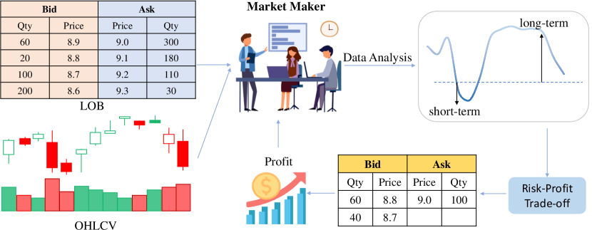
Figure 1: Workflow of professional human market makers.

The insight of IMM comes from the following inspiration: considering the workflow of a skilled human market maker (Figure 1), the professional first gathers both micro- and macro-level market information. The former aids in assessing market liquidity, while the latter contributes to evaluating adverse selection risks. Subsequently, he/she predicts short-term and long-term market trends based on these market information. Afterwards, he/she trade off between risks and profits according to their risk preference, leading to the ultimate trading decision ( the multiple prices and volumes of the quotes). Within numerous successful trading firms, this workflow plays a pivotal role in deriving robust and profitable MM strategies. Furthermore, beyond learning from interactions with the environment, extracting trading knowledge from experts presents an appealing method for mining profitable patterns (Ding et al. 2018). Leveraging expert data is a favorable approach to improve the exploration ability of RL algorithms(Sun, Bagnell, and Boots 2018; Mendonca et al. 2019).

Motivated by these inspirations, IMM integrates a state representation learning unit (SRLU) with an imitative RL unit (IRLU) to facilitate efficient policy learning for MM. Our primary contributions can be summarized as follows:

• IMM introduces effective state and action representations adeptly encoding multi-price level order information. These representations are well-suited for the MM environment, enabling the implementation of order stacking. Furthermore, IMM incorporates multi-granularity predictive signals as auxiliary variables, and employs a temporal convolution and spatial attention (TCSA) network to distill valuable representations from noisy market data.

• IMM utilizes trading knowledge from experts to facilitate effective exploration in the complex trading environment. To meet various risk preferences, IRLU trains customized agents by adjusting utility parameters of a specially crafted reward function.

• Through extensive experiments on four real-world financial futures datasets, we demonstrate that IMM significantly outperforms many baseline methods in relation to both risk-adjusted returns and adverse selection ratios. We underscore IMM’s practical applicability to MM through a series of comprehensive exploratory and ablative studies.

Related Work

Traditional Finance Methods

Traditional approaches for MM in the finance literature (Amihud and Mendelson 1980; Glosten and Milgrom 1985; Avellaneda and Stoikov 2008; Guéant, Lehalle, and Fernandez-Tapia 2012) consider MM as a stochastic optimal control problem that can be solved analytically. For example, the Avellaneda–Stoikov (AS) model (Avellaneda and Stoikov 2008) assumes a drift-less diffusion process for the mid-price evolution, then uses the Hamilton-Jacobi-Bellman equations to derive closed-form approximations to the optimal quotes. On a related note, (Guéant, Lehalle, and Fernandez-Tapia 2012) consider a variant of the AS model with inventory limits. However, such methods are typically predicated on a set of strong assumptions, and employ multiple parameters that need to be laboriously calibrated on historical data. It seems promising to consider more advanced methods such as RL that enables learning directly from data in a model-free fashion.

RL-based Methods

Recent years have witnessed a strong popularity of (deep) RL in the field of quantitative trading (Chan and Shelton 2001; Cartea, Donnelly, and Jaimungal 2015; Patel 2018; Zhong, Bergstrom, and Ward 2020; Fang et al. 2021; Niu, Li, and Li 2022; Sun et al. 2023).

The majority of the RL-based MM approaches adopts a single-price level strategy. Among those studies, several methods proposed defining the action space in advance (Spooner et al. 2018; Xu, Cheng, and He 2022; Sadighian 2019). Several researchers utilized a ”half-spread” action space which chooses a continuous half spread on each side of the book (Glosten and Milgrom 1985; Jumadinova and Dasgupta 2010; Cartea, Jaimungal, and Penalva 2015; Lim and Gorse 2018; Guéant and Manziuk 2019). Unfortunately, when actually implementing such a strategy, to change the half spread on each side of the book, it is necessary to actively cancel orders at each time step and place new orders at the new level. This results in frequent unnecessary order cancellations, leading to queue position losing (Jerome, Palmer, and Savani 2022).

To overcome this limitation, ladder strategies, which place a unit of volume at all prices in two price intervals, one on each side of the book, has been adopted(Chakraborty and Kearns 2011; Abernethy and Kale 2013). The latest work uses variants of this strategy to construct multi-price level MM policies. The $DRL_{OS}$ (Chung et al. 2022) agent decides whether to retain one unit of volume on each price level, and the beta policy (Jerome, Palmer, and Savani 2022) allows for flexibility in the distribution of order volumes.

However, to provide more accurate trading decisions, multi-price level strategy involves a much complex fine-grained action space (multi-level price and quantity). Little attention has been paid to inefficient exploration problem due to the complex action space of multi-price strategies. While have shown great promise, these approaches might be limited to achieve efficient exploration, particularly in highly dynamic and complex market environments.

Imitative Market Maker (IMM)

This section introduces the proposed IMM framework. We start with introducing a novel state/action space and illustrating the transition dynamics of MM procedure that accommodates multi-price level order stacking. Subsequently, we elaborate on the SRLU which aims at forecasting multi-granularity signals while extracting valuable representations from the noisy market data. Lastly, we outline the MM policy learning approach, which incorporates the RL and imitation learning objectives.

Multi-Price Level Strategy

In this subsection, we introduce a novel action space specially crafted to define the multi-price level MM strategy.

In practical MM scenarios, market participants analyze many quantities before sending orders, among which the most important one is the distance between their target price and the ”reference market price” $p_{ref}$, typically the midprice (Huang, Lehalle, and Rosenbaum 2013). The LOB can be formulated as a $2K$-dimensional vector, where $K$ denotes the number of available limits on each side. Notably, $p_{ref}$ serves as the LOB’s central point, thereby determining the positions of the 2K limits $Q_{\pm i}$, where $Q_{\pm i}$ represents the limit at the distance $i-0.5$ ticks to the right ($+i$) or left ($-i$) of $p_{ref}$. It is assumed that buy limit orders are placed on the bid side, and sell ones on the ask side. The queue length at $Q_{i}$ is denoted as $l_{i}$.

Most existing MM methods adopt the market midprice as $p_{ref}$ to encode the LOB. However, the specific price linked with level $i$ may experience frequent shifts due to the dynamic fluctuations in the midprice. Whenever alterations occur in $p_{ref}$, the corresponding $l_{i}$ instantaneously transitions to the value of one of its adjacent neighbors. This hinders the extraction of valid micro-market information from LOB. The necessity arises to define a stable reference price.

To this end, this paper formulates $p_{ref}$ in the subsequent manner: Firstly, we set up a reference price $\tilde{p}_{ref}$ that follows the midprice. Specifically, in instances where the market spread is odd, $\tilde{p}_{ref,t}:=m_{t}=\frac{ask_{t}+bid_{t}}{2}$. When the spread is even, $\tilde{p}_{ref,t}:=m_{t}\pm\frac{\text{price tick}}{2}$, with the selection of the sign based on proximity to the prior value. Afterwards, at the beginning of an episode, we set $p_{ref,0}=\tilde{p}_{ref,0}$. Then when the midprice $m_{t}$ increases (or decreases), only if $l_{-1,t}=0$ (or $l_{1,t}=0$), $p_{ref,t}$ is updated to $\tilde{p}_{ref,t}$. Consequently, changes of $p_{ref}$ are possibly caused by one of the three following events: (1) The insertion of a buy/sell limit order within the bid-ask spread while $Q_{1}$/$Q_{-1}$ is empty. (2) A cancellation of the last limit order at one of the best price. (3) A market order that consumes the last limit order at one of the best offer queues. Note that within our framework, the LOB accommodates empty limits, as depicted in Figure 2. In this way, we obtain a more stable $p_{ref}$, enabling effective encoding of LOB and multi-price level orders.

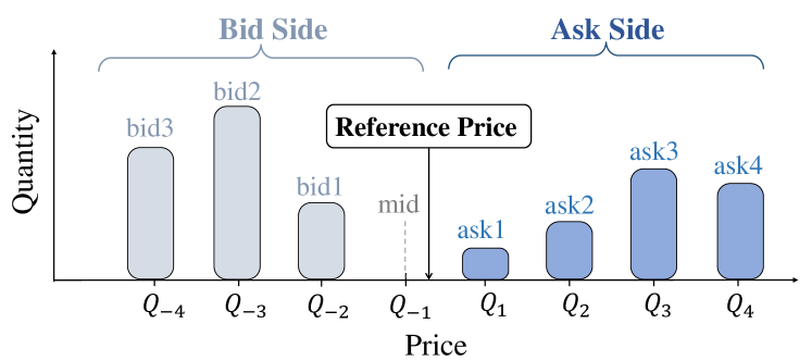
Figure 2: Limit order book and the reference price. In this instance, $Q_{-1}$ is an empty limit.

State Space

With such a stable reference price, IMM then effectively encodes both micro-level market information and multi-price level orders. To mitigate adverse selection risk, the state space necessitates the inclusion of macro-level market information¹. At time step $t$, the IMM agent observes the state formulated by:

$$\bm{s}_{t}=(\bm{s}_{t}^{m},\bm{s}_{t}^{s},\bm{s}_{t}^{p}),$$ (1)

where $\bm{s}_{t}^{m}$ denotes the market variables encoding the current market status; $\bm{s}_{t}^{s}$ denotes the signal variables, including multi-granularity auxiliary predictive signals; $\bm{s}_{t}^{p}$ denotes the private variables, including: the current inventory $z_{t}$, the queue position information and volume of the agent’s orders that rests on the LOB, denoted by $s_{t}^{q}=(q_{t}^{-K}...,q_{t}^{-1},q_{t}^{1},...,q_{t}^{K})$ and $s_{t}^{v}=(v_{t}^{-K}...,v_{t}^{-1},v_{t}^{1},...,v_{t}^{K})$ respectively. Here $q_{i}$ and $v_{i}$ denote the queue position information and volume at price level $i$ respectively. Suppose there are $m_{i}$ orders resting at level $i$ placed at different time step. The queue position value of the $j$-th order at level $i$ can be defined as $q_{t}^{i,j}=\frac{l_{i}^{front,j}}{l_{t}^{i}},$ where $l_{i}^{front,j}$ is the queue length in front of this order. Thus the queue position value at price level $i$ can be defined as the volume weighted average of the queue position values of the $m_{i}$ orders: $q_{t}^{i}=\sum\frac{l_{t}^{front,i,j}}{l_{t}^{i}}\frac{v_{t}^{i,j}}{l_{t}^{i}}.$ Through covering the information of the current quotes in states, the IMM learns to avoid frequent order cancellations and replacements.

Action Space

Reserving good queue positions beyond best bid/ask levels holds advantages of controlling adverse selection and non-execution risks. Therefore, practitioners tend to deploy order stacking strategies that place limit orders at multiple price levels in advance. IMM introduces an action encoding that expresses the complex multi-price level strategies within a low-dimensional space. At time step $t$, the action $\bm{a}_{t}$ is defined as

$$\bm{a}_{t}=(m_{t}^{*},\delta_{t}^{*},\bm{\phi}^{bid}_{t},\bm{\phi}^{ask}_{t}),$$ (2)

where $m_{t}^{*}$ and $\delta_{t}^{*}$ denote the desired quoted midprice w.r.t $p_{ref}$ and spread respectively. This implies that the agent’s target selling price is no lower than $m_{t}^{*}+\delta_{t}^{*}/2$, and the highest buying price is $m_{t}^{*}-\delta_{t}^{*}/2$. $\bm{\phi}^{bid}_{t}$ and $\bm{\phi}^{ask}_{t}$ represent parameter vectors that govern the volume distribution of the multi-level quotations. An instance of diverse two-price level actions is illustrated in Figure 3. By adopting such action formulation, the agent gains the flexibility to determine both the width and asymmetry of the quotes with respect to the reference price.

We formulate MM as an episodic RL task. The MM procedure allows for multi-price level order stacking, as specified below: (1) Choose a random start time for the episode and initialize the environment and the simulator. (2) Let the agent choose the desired volumes and price levels at which the agent would like to be positioned in the LOB. (3) Turn these desired positions into orders, including cancelling orders from levels with too much volume and placing new limit orders. (4) Match the orders in market-replay simulator according to the price-time priority. (5) Update the agent’s cash and inventory of the traded asset and track profit and loss. (6) Repeat steps (2-4) until the episode terminates. A picture illustration can be found in Figure LABEL:fig:env in the supplementary material.

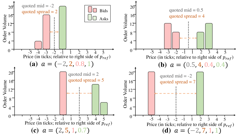
Figure 3: Illustration of action space. Consider a scenario where an agent positions two-level orders on both sides of the LOB, $\phi_{t}^{ask}$ (the green number) determines the ratio of volume placed at the two adjacent ask price levels (heights of the green bars).

State Representation Learning Unit (SRLU)

Signal Generation

To leverage the labels containing future information, IMM pretrains supervised learning (SL) models to generate both short- and long-term trend signals¹. The choice of the SL models are flexible. In this paper, we adopt LightGBM (Ke et al. 2017), a highly robust ensemble model based on decision trees, to generate four multi-granularity trend signals denoted by $(y^{20},y^{120},y^{240},y^{600})$, which are the labels of price movement trend after $1/6,1,2,5$ minutes respectively. While training the RL policy, the parameters of the pre-trained predictors are frozen, and the outputs constitute the auxiliary signal variables $\bm{s}^{s}$.

Attention-based Representation Learning

Deep RL algorithms usually suffer from the low data-efficiency issue. Besides the auxiliary signal prediction, we propose an temporal convolution and spatial attention (TCSA) network to extract additional effective representations from the noisy market data $\bm{x}$. The structure of TCSA is depicted in Figure 4.

The proposed approach IMM first utilizes a temporal convolution network (TCN) (Yu and Koltun 2015) block to extract the time-axis relations in the data. Compared to recurrent neural networks, TCN has several appealing properties including parallel computation and longer effective memory. After conducting TCN operations on $\bm{x}\in\mathbb{R}^{F\times L}$ along the time axis, we obtain an output tensor denoted by $\hat{\bm{H}}\in\mathbb{R}^{F\times L}$, where $F$ is the dimension of features, and $L$ is the temporal dimension.

Afterward, IMM adopts an attention mechanism (Vaswani et al. 2017) to handle the spatial relationships among different features. Given the output vector of TCN, we calculate the spatial attention weight as $\hat{\bm{S}}=\bm{V}\cdot\text{sigmoid}\big{(}(\hat{\bm{H}}\bm{W}_{1})\bm{\cdot}(\hat{\bm{H}}\bm{W}_{2})^{T}+\bm{b}\big{)},$ where $\bm{W}_{1},\bm{W}_{2}\in\mathbb{R}^{L}$, and $\bm{V}\in\mathbb{R}^{F\times F}$ are parameters to learn, $\bm{b}\in\mathbb{R}^{F\times F}$ is the bias vector. The matrix $\bm{\hat{}}{S}\in\mathbb{R}^{F\times F}$ is then normalized by rows to represent the correlation among features: $\bm{S}_{i,j}=\frac{\exp(\hat{\bm{S}}_{i,j})}{\sum_{u=1}^{F}\exp(\hat{\bm{S}}_{i,u})},\forall 1\leq i\leq F.$

We adopt the ResNet (He et al. 2016) structure to alleviate the vanishing gradient problem in deep learning. The final representation abstracted from $\bm{x}$ is denoted by $H=S\times\hat{\bm{H}}+\bm{x}$, and it is then translated to a vector with dim $F^{\prime}$ using a fully connected layer: $\bm{s}^{m}=\text{sigmoid}(W_{4}\cdot\text{ReLU}(\bm{H}W_{3}+\bm{b}_{3})+\bm{b}_{4}).$ The representation $\bm{s}^{m}$ is concatenated with the signal state $\bm{s}^{s}$ and private state $\bm{s}^{p}$.

RB

FU

CU

AG

EPnL[$10^{3}$]

MAP[unit]

PnLMAP

EPnL[$10^{3}$]

MAP[unit]

PnLMAP

EPnL[$10^{3}$]

MAP[unit]

PnLMAP

EPnL[$10^{3}$]

MAP[unit]

PnLMAP

FOIC

3.23 $\pm$ 4.35

255 $\pm$ 111

14 $\pm$ 22

-7.79 $\pm$ 9.25

238 $\pm$ 135

-43 $\pm$ 56

-33.05 $\pm$ 27.63

206 $\pm$ 141

-161 $\pm$ 224

-48.39 $\pm$ 28.83

189 $\pm$ 154

-250 $\pm$ 335

LIIC

2.26 $\pm$ 3.32

123$\pm$32

20 $\pm$ 29

-6.89 $\pm$ 6.66

115$\pm$ 30

-66 $\pm$ 69

-24.19 $\pm$ 14.83

150 $\pm$ 20

-164 $\pm$ 513

-38.9 $\pm$ 26.2

142 $\pm$ 45

-302 $\pm$ 243

LTIIC

9.16 $\pm$ 4.87

65 $\pm$ 6

139 $\pm$ 68

8.26 $\pm$ 2.64

52 $\pm$ 3

160 $\pm$ 50

-16.74 $\pm$ 15.81

112 $\pm$ 109

-190 $\pm$ 203

-32.57 $\pm$ 22.8

128 $\pm$ 22

-264 $\pm$ 166

$RL_{SD}$

4.36 $\pm$ 1.64

38 $\pm$ 4

114 $\pm$ 38

7.31 $\pm$ 5.38

76 $\pm$ 29

90 $\pm$ 46

-19.7 $\pm$ 17

214 $\pm$ 109

-92 $\pm$ 298

-25.43 $\pm$ 23.83

107 $\pm$ 37

-237 $\pm$ 235

$DRL_{OS}$

8.22 $\pm$ 3.70

51 $\pm$ 4

156 $\pm$ 61

11.03 $\pm$ 13.87

37 $\pm$ 3

30 $\pm$ 36

-18.9 $\pm$ 18.02

647 $\pm$ 2367

-99 $\pm$ 147

-28.39 $\pm$ 27.92

169 $\pm$ 154

-167 $\pm$ 135

IMM

16.46 $\pm$ 9.10

96$\pm$ 13

165 $\pm$ 74

28.10 $\pm$ 10.27

102 $\pm$ 14

274 $\pm$ 89

-4.86 $\pm$ 10.17

111 $\pm$ 28

-43 $\pm$ 87

-14.5 $\pm$ 20.2

102 $\pm$ 14

-274 $\pm$ 89

Table 1: The comparison results of the proposed method and the benchmarks.

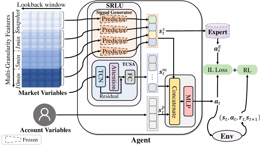
Figure 4: The proposed IMM learning framework.

Imitative Reinforcement Learning Unit (IRLU)

A Signal-Based Expert

To guide efficient exploration, we define a linear suboptimal rule-based expert strategy named Linear in Trend and Inventory with Inventory Constraints (LTIIC), which is commonly used by human experts. Readers might employ other effective expert strategies if available. $LTIIC(a,b,c,d)$ corresponds to a strategy where a market maker adjusts its quote prices based on both its inventory level and trend prediction signals. If $-d\leq z_{t}\leq d$ at time $t$, the ask and bid orders are placed with prices:

$$\left\{\begin{aligned} ask_{t}^{q}&=&m_{t}+a+b\cdot z_{t}+c\cdot\hat{y}_{t},\\ bid_{t}^{q}&=&m_{t}-a+b\cdot z_{t}+c\cdot\hat{y}_{t},\\ \end{aligned}\right.$$ (3)

where $a$, $b$, $c$ and $d$ are predetermined parameters, $m_{t}$ stands for the midprice of the LOB, $z_{t}$ represents the inventory, and $\hat{y}_{t}\in\{-1,0,1\}$ signifies a short-term predictive trend signal. The insights of LTIIC strategy lies in that during a short-term upward market trend, ask-side limit orders are more likely to be executed than bid-side ones. A logical approach involves implementing a narrow half-spread on the bid side and a broader half-spread on the ask side, thus reducing the risk exposure due to adverse selection. Simultaneously, the trader adjusts parameter $b$ to regulate the inventory level, while $a$ determines the quoted spread. In cases where $z_{t}>=d$ or $z_{t}<=-d$, only orders on the side opposite to the inventory are posted.

Policy Learning

We utilized the actor-critic RL framework (Konda and Tsitsiklis 1999), where the critic evaluates the action taken by the actor by computing the value function, and the actor (policy) is optimized to maximize the value output by the critic. To improve the sample efficiency, we use the off-policy actor-critic method TD3 (Fujimoto, Hoof, and Meger 2018) as the base learner, and the policy $\pi$ is updated with the deterministic policy gradient (Silver et al. 2014):

$$\pi=\arg\max_{\pi}\mathbb{E}_{(\bm{s},a)\sim D}\big{[}Q(\bm{s},\pi(\bm{s}))\big{]},$$ (4)

where $Q$ is a value function approximating the expected cumulative reward, $Q(\bm{s}_{t},\bm{a}_{t})=\mathbb{E}[\sum_{i=t}^{T}\gamma^{i-t}r_{i}|\bm{s}_{t},\bm{a}_{t}]$.

In Equation (4), $D$ denotes the replay buffer collected by a behavior policy, which is generated by adding some noise to the learned policy $\pi$. Following the TD3 method (Fujimoto, Hoof, and Meger 2018), the value function $Q$ is optimized in a twin delayed manner with the data sampled from both the replay buffer $D$ and expert dataset $D_{E}$.

Since the high-dimensional state space, the complex action space, and the stochastic trading environment induce a hard exploration problem, learning with a pure RL objective in Equation (4) is extremely difficult. To promote the policy learning in such complex trading environment, we propose to augment the RL method with the objective of imitating the quoting behavior in an expert dataset $D_{E}$ as:

$$\pi= \arg\max_{\pi}\mathbb{E}_{(\bm{s},a)\sim D}\big{[}Q(\bm{s},\pi(\bm{s}))\big{]}-\mathbb{E}_{(\bm{s},\hat{a})\sim D_{E}}\big{[}\lambda\cdot(\pi(\bm{s})-\hat{a})^{2}\big{]},$$ (5)

where $\lambda$ is a scaling coefficient that balances maximizing the Q values and minimizing the behavior cloning (BC) loss. We set $\lambda$ decrease with the growth of the training steps.

As the expert dataset contains reasonable suboptimal MM behaviors, the agent benefits from the imitation learning techniques through abstracting advanced trading knowledge. Thus the proposed method could achieve more efficient exploration and policy learning in the highly stochastic market environment compared to the RL methods without imitation learning.

Reward Function for Diverse Utilities

The decision process of the market makers is subject to several trade-offs, including probability of execution and spread, inventory risk, and compensation from the exchange. To meet the diverse utilities of market makers, three factors are proposed to be considered:

Profit and loss ($PnL$). PnL is a natural choice for the problem domain, comprising a realized $PnL$ term (left part) and a floating $PnL$ term (right part), given by:

$$PnL_{t}=\bigg{(}\sum_{i\in A_{t}}p^{a}_{i}\cdot v^{a}_{i}-\sum_{j\in B_{t}}p^{b}_{j}\cdot v^{b}_{j}\bigg{)}+(p_{t+1}-p_{t})\cdot z_{t+1},$$ (6)

where $p$ denotes the market midprice; $p^{a},v^{a},p^{b},v^{b}$ represents the price and volume of the filled ask (bid) orders respectively; $z$ signifies the current inventory, with $z>0$ when the agent holds a greater long position than short.

Truncated Inventory Penalty. To mitigate inventory risk, it is reasonable to introduce an additional inventory dampening term. Considering that advanced market makers may choose to hold a non-zero inventory to exploit clear trends while capturing the spread, an enhanced approach involves applying the dampening term solely to higher-risk inventory levels:

$$IP_{t}=-\eta|z_{t}|\cdot\mathbb{I}(|z_{t}|>C),$$ (7)

A penalty for inventory holding is applied solely when the inventory $z_{t}$ surpasses a constant $C$.

The Market Makers’ compensation from the exchange constitutes a primary revenue stream for numerous market makers (Fernandez-Tapia 2015). Therefore, ensuring a substantial volume of transactions to secure compensations holds significant importance for a variety of MM companies. To this end, a bonus term is incorporated to encourage transactions of the agent:

$$C_{t}=\beta\bigg{(}\sum_{i\in A_{t}}p^{a}_{i}\cdot v^{a}_{i}+\sum_{j\in B_{t}}p^{b}_{j}\cdot v^{b}_{j}\bigg{)},$$ (8)

Ultimately, by appropriately tuning the parameters $\eta$ and $\beta$ based on personalized utilities, IMM ensures alignment with the requirements of a broad spectrum of market makers, employing the combination of these three categories of rewards:

$$\mathcal{R}(\bm{s}_{t},\bm{a}_{t},\bm{s}_{t+1})=PnL_{t}+C_{t}+IP_{t}.$$ (9)

Experiments

Experimental Setup

We conduct experiments on four datasets comprised of historical data of the spot month contracts of the $FU$, $RB$, $CU$ and $AG$ futures from the Shanghai Futures Exchange. The data consists of the 5-depth LOB and aggregated trades information associated with a $500$-milliseconds real-time financial period. We use the data from July 2021 to March 2022 (126 trading days) for training with $20\%$ as the validation set, and test model performance on April 2022 $\sim$ July 2022 (60 trading days). In each episode, the agent adjusts its 2-level bids and asks every $500$ milliseconds, with a fixed total volume $N=20$ units on each side. The episode length is set to 1.5 trading hour, with $T=10800$ steps.

Benchmarks

We compare IMM with three rule-based benchmarks and two state-of-the-art RL-based approaches:

1. FOIC represents a Fixed Offset with Inventory Constraints strategy introduced by (Gašperov and Kostanjčar 2021). $FOIC(d)$ refers to the strategy that posts bid (ask) orders at the current best bid (ask) while adhering to the inventory constraint $d$.

2. LIIC. A Linear in Inventory with Inventory Constraints strategy (Gašperov and Kostanjčar 2021) corresponds to the strategy where a market maker adjusts its quote prices based on its inventory level. The quotes of LIIC can be formulated as $LTIIC(a,b,c=0,d)$ using Equation (3).

3. LTIIC is the expert adopted in IMM.

4. $\bf RL_{DS}$ refers to a RL-based single-price level strategy proposed by (Spooner et al. 2018).

5. $\bf DRL_{OS}$ refers to a state-of-the-art RL-based multi-price level strategy proposed in (Chung et al. 2022). The agent decides whether to retain one unit of volume on each price level, not allowing for volume distribution across all price levels.

Evaluation metrics

We adopt four financial metrics to assess the performance of a MM strategy:

• Episodic PnL is a natural choice to evaluate the profitability of a MM agent, since there is no notion of starting capital in MM procedure: $EPnL_{T}=\sum_{t=1}^{T}PnL_{t}.$

• Mean Absolute Position (MAP) accounts for the inventory risk, defined as: $MAP_{T}=\frac{\sum_{t=1}^{T}|z_{t}|}{\sum_{t=1}^{T}1\cdot\mathbb{I}(|z_{t}|>0)}$.

• Return Per Trade (RPT) evaluates the agent’s capability of capturing the spread. It is normalized across different markets by the average market spread $\overline{\delta^{m}}$ .

  $$RPT_{T}=\bigg{(}\frac{\sum_{i\in A_{T}}p_{i}^{a}*n_{i}^{a}}{\sum_{i\in A_{T}}n_{i}^{a}}-\frac{\sum_{j\in B_{T}}p_{j}^{b}*n_{j}^{b}}{\sum_{j\in B_{T}}n_{j}^{b}}\bigg{)}\bigg{/}\overline{\delta^{m}}.$$

• PnL-to-MAP Ratio (PnLMAP) simultaneously considers the profitability and the incurred inventory risk of a market making strategy: $PnLMAP_{T}=\frac{EPnL_{T}}{MAP_{T}}$.

Comparison Results with Baselines

For a fair comparison, we tune the hyper-parameters of these methods for the maximum PnLMAP_T value on the validation dataset. The comparison results of IMM and the benchmarks on the four test datasets are given in Table 1 and supplementary materials. These comparison results indicate that the proposed approach significantly outperforms the benchmarks in terms of both profitability and risk management.

As demonstrated in Table 1, on the RB dataset, the proposed method attains the highest terminal wealth as well as risk-ajusted return, albeit with a slightly elevated MAP in comparison to the expert and the two RL-based methods. Besides, the two multi-price level RL-based agents $DRL_{OS}$ and IMM outperform the single-price level method $RL_{DS}$, indicating the superiority of mult-price level strategy. On the FU dataset, IMM not only achieves the highest terminal wealth but also demonstrates the most favorable return-to-risk performance and spread-capturing ability, while maintaining the second-lowest inventory level. The RL-based strategies achieve commendable performance compared to the rule-based strategies which fail to make profits in most trading days. Moreover, it is observed that IMM acquires a competitive MM strategy, which attains stable dividends with profits (the pink line) while sustaining the inventory at a tolerable low level (the compact blue region) in a violate market, as illustrated in the left part of Figure 5. The inventory fluctuates around zero, which is a desirable behaviour. Remarkably, since IMM does not force the agent to place opposite-side orders to clear its inventory, it is a quite appealing result to see IMM accomplishes automatic inventory control based on state-derived information. Even in the challenging MM tasks on CU and AG markets which show lower market liquidity, the proposed method significantly outperforms the benchmarks in terms of the terminal wealth and risk-adjsted return.

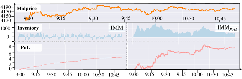
Figure 5: Performance of IMM and IMM${}_{-}PnL$ on FU on Jun. 14th, 2022.

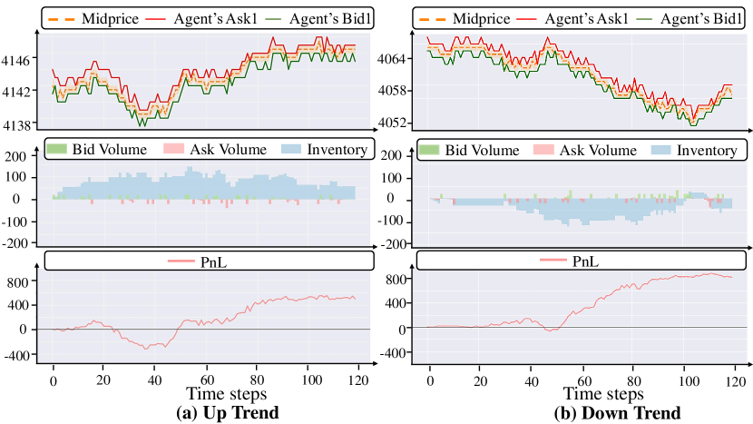
Figure 6: 1-minute Cases. IMM performs well in both up- and down-trend markets.

Model Component Ablation Study

To investigate the effectiveness of the model component, we compare the proposed IMM with its five variations summarized in Table 2, and the results are listed in Table 3.

Effectiveness of the State Representations

To examine the efficacy of the proposed state representations, we analyse the performance of three IMM_SL(⋅) models. Based on Table 3, it is evident that introducing multi-granularity signals as auxiliary observations holds significant importance in enhancing the MM strategy’s performance. Figure 6 visualizes the behaviour of IMM during two 1-minute periods with different trends on FU test dataset. As demonstrated in Figure 6(a), benefiting from the auxiliary signals, the IMM agent anticipates an ascending price trend and proactively maintains a long position prior to the onset of a short-term bullish trend (steps 0-40). With the trend terminates (step 70-120), the agent gradually reduces its inventory through placing orders with narrow ask-side half-spread and broad bide-side one w.r.t the market midprice. Similarly, the IMM agent demonstrates proficient behavior in downside markets as shown in 6(b). Combined with the adverse select ratio depicted in Figure 7, it can be concluded that IMM has learned to mitigated adverse selection risk.

For a deeper investigation into the role of auxiliary signals in improving performance, we calculated the adverse selection ratio as $adv\_ratio=\frac{\text{\# adverse fills}}{\text{\# fills in last interval}}.$ Here adverse fills refers to limit bid (ask) orders which are executed shortly before a downward (upward) movement of the best bid (ask) price. As if the best bid price would have gone down, it might have better to wait the next bid price level (Chung et al. 2022). Based on Figure 7(a), we can deduce that the multi-granularity predictive signals play a vital role in mitigating adverse selections. That might because they provide effective information about market conditions, which enables more flexible trade-off between spread-capturing and trend-chasing. Moreover, Figure 7(b) demonstrates that the information regarding multi-price level orders additionally contributes to enhancing the fills count by minimizing frequent cancellations and preserving queue positions.

Models	QuotesInfo	Signals	TCSA	RL	IL
IMMSL(m)	O	O	X	O	O
IMMSL(s)	O	X	O	O	X
IMMSL(q)	X	O	O	O	O
IMMBC(0)	O	O	O	O	X
IMMBC(1)	O	O	O	X	O

Table 2: Five variations of the proposed IMM.

	EPnL[$10^{3}$]	MAP[unit]	PnLMAP	SR
IMMSL(m)	10.57 $\pm$ 8.63	74 $\pm$ 41	142 $\pm$ 39	1.22
IMMSL(s)	7.83 $\pm$ 3.64	49 $\pm$ 5	159 $\pm$ 46	2.15
IMMSL(q)	10.20 $\pm$ 9.72	74 $\pm$ 47	104 $\pm$ 56	1.05
IMMBC(0)	14.67 $\pm$ 5.11	85 $\pm$ 5	172 $\pm$ 57	2.87
IMMBC(1)	8.22 $\pm$ 3.70	51 $\pm$ 4	156 $\pm$ 61	2.22
IMM	28.097 $\pm$ 10.27	103 $\pm$ 15	274 $\pm$ 89	2.80

Table 3: Comparison results of ablation study on FU dataset.

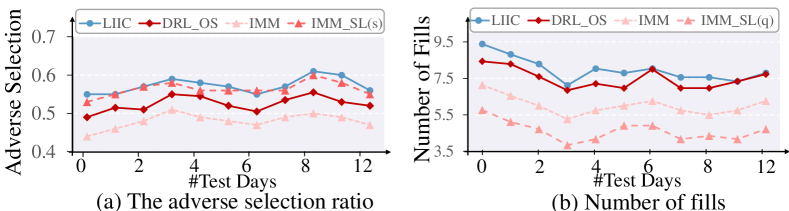
Figure 7: The daily adverse selection ratios and normalized number of fills.

Effectiveness of the IRLU

The comparison results between IMM_BC(⋅) and IMM provide empirical evidence of the importance of extracting additional knowledge from the expert and conducting efficient exploration, particularly for challenging financial tasks. Besides, IMM outperforms the expert LTIIC strategy a lot. As the RL agent faces challenges in identifying a viable trading approach and sustaining it over multiple steps during the initial training phase. Training while pursuing the imitation learning objective facilitates the agent in obtaining favorable rewards and drawing valuable lessons from these experiences.

Effects of Reward Functions

To investigate whether the proposed reward function meets different utilities, we train IMM that with three different rewards: The IMM_PNL mehtod trains IMM using the PnL reward ($\eta,\beta=0$); The IMM_PNL+C method trains IMM with the combination of the PNL and compensation reward ($\eta=0,\beta>0$); The IMM_PNL+IP method trains IMM with the combination of the PNL and truncated inventory penalty reward ($\eta>0,\beta=0$). The hyperparameters resulting in the maximum PnLMAP value on the validation dataset are chosen for these models. The results on the FU dataset are outlined in Table 4. Here the metric #T signifies the number of fills normalized by the episode length.

	EPnL[$10^{3}$]	MAP[unit]	PnLMAP	#T
IMMPnL	58.76 $\pm$ 94.43	2156 $\pm$ 655	31 $\pm$ 48	4.43 $\pm$ 0.94
IMMPnL+C	42.86 $\pm$ 123.04	2041 $\pm$ 465	27 $\pm$ 68	4.85 $\pm$ 1.09
IMMPnL+IP	73.07 $\pm$ 53.83	756 $\pm$ 289	90 $\pm$ 46	4.42 $\pm$ 0.96
IMM	28.097 $\pm$ 10.27	103 $\pm$ 15	274 $\pm$ 89	5.15 $\pm$ 1.19

Table 4: Performance of IMM variations trained with different reward preferemces on FU dataset.

As shown in Table 4, the IMM_PNL strategy tends to have the most substantial inventory risk exposure. We depict an example of the intra-day performance of the IMM_PNL policy in the right part of Figure 5. We observe that the IMM_PNL agent learns to chase trends through maintaining a large inventory ($>1000$). This result in poor out-of-sample performance with large variance. Therefore, the truncated inventory penalty term proves crucial in curbing blind trend-chasing tendencies.

The IMM_PnL+C strategy also grapples with elevated inventory risk, yet it achieves a greater number of transactions #T compared to IMM_PnL. The IMM_PnL+IP strategy attains the highest average terminal wealth and the return per trade metric, but concurrently records the lowest #T, a circumstance that may be less advantageous for risk-averse market makers. The strategy trained with the proposed reward significantly improve the return-to-risk performance with the lowest MAPs, as well as a larger #T, compared to the IMM_PnL+IP strategies. Althoug having the lowest average terminal wealth, the proposed IMM strategy acts very stably and might be the most favorable policy among these four policies for a risk-averse market maker. Besides, note that the proposed strategy has a largest #T, it could receive more compensation from the exchange.

Conclusion

In this paper, we propose IMM, a novel RL-based approach aimed at efficiently learning multi-price level MM policies. IMM first introduces efficient state and action representations. Subsequently, it pre-train a SL-based prediction model to generate multiple trend signals as effective auxiliary observations. Futhermore, IMM utilizes a TCSA network to handle the temporal and spatial relationships in noisy financial data. Through abstracting trading knowledge from a sub-optimal expert meanwhile interacting with the environments, IMM explores the state and action spaces efficiently. Experiments on four futures markets demonstrate that IMM outperforms the benchmarks, and further ablation studies verify the effectiveness of the components in the proposed method.

References

- Abernethy and Kale (2013) Abernethy, J. D.; and Kale, S. 2013. Adaptive Market Making via Online Learning. In NIPS.
- Amihud and Mendelson (1980) Amihud, Y.; and Mendelson, H. 1980. Dealership market: Market-making with inventory. Journal of Financial Economics, 8: 31–53.
- Avellaneda and Stoikov (2008) Avellaneda, M.; and Stoikov, S. 2008. High Frequency Trading in a Limit Order Book. Quantitative Finance, 8: 217–224.
- Cartea, Donnelly, and Jaimungal (2015) Cartea, Á.; Donnelly, R. F.; and Jaimungal, S. 2015. Enhancing trading strategies with order book signals. Applied Mathematical Finance, 25: 1 – 35.
- Cartea, Jaimungal, and Penalva (2015) Cartea, Á.; Jaimungal, S.; and Penalva, J. S. 2015. Algorithmic and High-Frequency Trading.
- Chakraborty and Kearns (2011) Chakraborty, T.; and Kearns, M. 2011. Market making and mean reversion. In ACM Conference on Economics and Computation.
- Chan and Shelton (2001) Chan, N. T.; and Shelton, C. R. 2001. An Electronic Market-Maker.
- Chung et al. (2022) Chung, G. Y.; Chung, M.; Lee, Y.; and Kim, W. C. 2022. Market Making under Order Stacking Framework: A Deep Reinforcement Learning Approach. Proceedings of the Third ACM International Conference on AI in Finance.
- Ding et al. (2018) Ding, Y.; Liu, W.; Bian, J.; Zhang, D.; and Liu, T.-Y. 2018. Investor-Imitator: A Framework for Trading Knowledge Extraction. Proceedings of the 24th ACM SIGKDD International Conference on Knowledge Discovery & Data Mining.
- Fang et al. (2021) Fang, Y.; Ren, K.; Liu, W.; Zhou, D.; Zhang, W.; Bian, J.; Yu, Y.; and Liu, T.-Y. 2021. Universal Trading for Order Execution with Oracle Policy Distillation. In AAAI.
- Fernandez-Tapia (2015) Fernandez-Tapia, J. 2015. Modeling, optimization and estimation for the on-line control of trading algorithms in limit-order markets. Ph.D. thesis.
- Fujimoto, Hoof, and Meger (2018) Fujimoto, S.; Hoof, H.; and Meger, D. 2018. Addressing function approximation error in actor-critic methods. In International conference on machine learning, 1587–1596. PMLR.
- Gašperov and Kostanjčar (2021) Gašperov, B.; and Kostanjčar, Z. 2021. Market Making With Signals Through Deep Reinforcement Learning. IEEE Access, 9: 61611–61622.
- Glosten and Milgrom (1985) Glosten, L. R.; and Milgrom, P. R. 1985. Bid, ask and transaction prices in a specialist market with heterogeneously informed traders. Journal of Financial Economics, 14: 71–100.
- Guéant, Lehalle, and Fernandez-Tapia (2012) Guéant, O.; Lehalle, C.-A.; and Fernandez-Tapia, J. 2012. Dealing with the inventory risk: a solution to the market making problem. Mathematics and Financial Economics, 7(4): 477–507.
- Guéant and Manziuk (2019) Guéant, O.; and Manziuk, I. 2019. Deep Reinforcement Learning for Market Making in Corporate Bonds: Beating the Curse of Dimensionality. Applied Mathematical Finance, 26: 387 – 452.
- He et al. (2016) He, K.; Zhang, X.; Ren, S.; and Sun, J. 2016. Deep residual learning for image recognition. In Proceedings of the IEEE conference on computer vision and pattern recognition, 770–778.
- Huang, Lehalle, and Rosenbaum (2013) Huang, W.; Lehalle, C.-A.; and Rosenbaum, M. 2013. Simulating and analyzing order book data: The queue-reactive model. Papers 1312.0563, arXiv.org.
- Jerome, Palmer, and Savani (2022) Jerome, J.; Palmer, G.; and Savani, R. 2022. Market Making with Scaled Beta Policies. Proceedings of the Third ACM International Conference on AI in Finance.
- Jumadinova and Dasgupta (2010) Jumadinova, J.; and Dasgupta, P. 2010. A Comparison of Different Automated Market-Maker Strategies.
- Ke et al. (2017) Ke, G.; Meng, Q.; Finley, T.; Wang, T.; Chen, W.; Ma, W.; Ye, Q.; and Liu, T.-Y. 2017. LightGBM: A Highly Efficient Gradient Boosting Decision Tree. In Proceedings of the 31st International Conference on Neural Information Processing Systems, NIPS’17, 3149–3157. Red Hook, NY, USA: Curran Associates Inc. ISBN 9781510860964.
- Konda and Tsitsiklis (1999) Konda, V.; and Tsitsiklis, J. 1999. Actor-critic algorithms. Advances in neural information processing systems, 12.
- Lim and Gorse (2018) Lim, Y.-S.; and Gorse, D. 2018. Reinforcement Learning for High-Frequency Market Making. In ESANN.
- Mendonca et al. (2019) Mendonca, R.; Gupta, A.; Kralev, R.; Abbeel, P.; Levine, S.; and Finn, C. 2019. Guided Meta-Policy Search. In Neural Information Processing Systems.
- Niu, Li, and Li (2022) Niu, H.; Li, S. K.; and Li, J. 2022. MetaTrader: An Reinforcement Learning Approach Integrating Diverse Policies for Portfolio Optimization. Proceedings of the 31st ACM International Conference on Information & Knowledge Management.
- Patel (2018) Patel, Y. 2018. Optimizing Market Making using Multi-Agent Reinforcement Learning. ArXiv, abs/1812.10252.
- Sadighian (2019) Sadighian, J. 2019. Deep Reinforcement Learning in Cryptocurrency Market Making. arXiv: Trading and Market Microstructure.
- Silver et al. (2014) Silver, D.; Lever, G.; Heess, N.; Degris, T.; Wierstra, D.; and Riedmiller, M. 2014. Deterministic policy gradient algorithms. In International conference on machine learning, 387–395. PMLR.
- Spooner et al. (2018) Spooner, T.; Fearnley, J.; Savani, R.; and Koukorinis, A. 2018. Market Making via Reinforcement Learning. In AAMAS.
- Sun et al. (2023) Sun, S.; Wang, X.; Xue, W.; Lou, X.; and An, B. 2023. Mastering Stock Markets with Efficient Mixture of Diversified Trading Experts. In Proceedings of the 29th ACM SIGKDD Conference on Knowledge Discovery and Data Mining, KDD ’23, 2109–2119. New York, NY, USA: Association for Computing Machinery. ISBN 9798400701030.
- Sun, Bagnell, and Boots (2018) Sun, W.; Bagnell, J. A.; and Boots, B. 2018. Truncated Horizon Policy Search: Combining Reinforcement Learning & Imitation Learning. ArXiv, abs/1805.11240.
- Vaswani et al. (2017) Vaswani, A.; Shazeer, N.; Parmar, N.; Uszkoreit, J.; Jones, L.; Gomez, A. N.; Kaiser, L.; and Polosukhin, I. 2017. Attention is All You Need. In Proceedings of the 31st International Conference on Neural Information Processing Systems, NIPS’17, 6000–6010. Red Hook, NY, USA: Curran Associates Inc. ISBN 9781510860964.
- Xu, Cheng, and He (2022) Xu, Z.; Cheng, X.; and He, Y. 2022. Performance of Deep Reinforcement Learning for High Frequency Market Making on Actual Tick Data. In AAMAS.
- Yu and Koltun (2015) Yu, F.; and Koltun, V. 2015. Multi-scale context aggregation by dilated convolutions. arXiv preprint arXiv:1511.07122.
- Zhong, Bergstrom, and Ward (2020) Zhong, Y.; Bergstrom, Y.; and Ward, A. R. 2020. Data-Driven Market-Making via Model-Free Learning. In IJCAI.