Lifted Algorithms for Symmetric Weighted First-Order Model Sampling

Abstract

Weighted model counting (WMC) is the task of computing the weighted sum of all satisfying assignments (i.e., models) of a propositional formula. Similarly, weighted model sampling (WMS) aims to randomly generate models with probability proportional to their respective weights. Both WMC and WMS are hard to solve exactly, falling under the #¶-hard complexity class. However, it is known that the counting problem may sometimes be tractable, if the propositional formula can be compactly represented and expressed in first-order logic. In such cases, model counting problems can be solved in time polynomial in the domain size, and are known as domain-liftable. The following question then arises: Is it also the case for weighted model sampling? This paper addresses this question and answers it affirmatively. Specifically, we prove the domain-liftability under sampling for the two-variables fragment of first-order logic with counting quantifiers in this paper, by devising an efficient sampling algorithm for this fragment that runs in time polynomial in the domain size. We then further show that this result continues to hold even in the presence of cardinality constraints. To empirically verify our approach, we conduct experiments over various first-order formulas designed for the uniform generation of combinatorial structures and sampling in statistical-relational models. The results demonstrate that our algorithm outperforms a start-of-the-art WMS sampler by a substantial margin, confirming the theoretical results.

1 Introduction

Given a propositional formula and a weight for each truth assignment, weighted model counting (WMC) aims to compute the cumulative weight of all satisfying assignments (i.e., models) of the input formula. A closely related problem to WMC is weighted model sampling (WMS), which samples models of the propositional formula, where the probability of choosing a model is proportional to its weight. These problems find applications in various domains, including machine learning [28, 30], probabilistic inference [5], statistics, planning and combinatorics [8, 38], and constrained random verification [2, 3, 32]. Unfortunately, both WMC and WMS are computationally challenging, falling within the #¶-hard complexity class [35, 9]. Nevertheless, a glimmer of hope emerges when the input propositional formula can be naturally and compactly represented using first-order logic. In such cases, the WMC problem may become tractable by exploiting the symmetries present in the problem.

Weighted first-order model counting (WFOMC) is a variant of WMC in first-order logic. In the context of WFOMC, we consider a function-free first-order sentence $\Gamma$ and a finite domain $\Delta$. A model of $\Gamma$ interprets each predicate in $\Gamma$ over $\Delta$ such that the interpretation satisfies $\Gamma$. First-order model counting (FOMC), the unweighted version of WFOMC, aims to compute the total number of models of $\Gamma$. For instance, the model count of $\forall x\exists y:R(x,y)$ over a domain of size $n$ is equal to $(2^{n}-1)^{n}$. In WFOMC, one further associates a real number called weight with atomic facts and their negations in the models, and defines the weight of a model as the product of the weights of its constituent facts. The WFOMC problem is then to calculate the weighted summation over all models of the formula $\Gamma$. Many real-world problems, including probabilistic inference and weight learning in various statistical-relational learning (SRL) models, can be directly reduced to WFOMC [42, 45].

An important advantage of WFOMC is the existence of domain-lifted (or simply lifted) algorithms for certain fragments of first-order logic, which are algorithms that have a polynomial runtime with respect to the domain size [39, 1, 23, 24]. In contrast to algorithms for WMC that operate on the propositional representation of the first-order sentence, lifted algorithms can provide an exponential acceleration as the domain size increases. The existence of lifted algorithms for WFOMC then raises an intriguing question: Are there likewise lifted algorithms for WMS variations in first-order logic?

In this work, we answer this question by studying the weighted first-order model sampling (WFOMS) problem. This problem, which is a sampling counterpart of WFOMC, aims to generate a model of the input first-order sentence $\Gamma$ based on a probability that is proportional to its weight. The WFOMS problem offers a natural reduction for a wide range of sampling problems without the necessity of converting them into WMS by grounding the input first-order sentence. Many problems relating to the generation of combinatorial structures can be readily formulated as WFOMS. For instance, suppose we are interested in uniformly sampling labeled 2-colored graphs with $n$ nodes, it is equivalent to solving the WFOMS problem on the sentence:

$$\forall x: \neg E(x,x)\ \land$$ (1)

$$\forall x\forall y: E(x,y)\Rightarrow E(y,x)\ \land$$

$$\forall x: Red(x)\lor Black(x)\ \land$$

$$\forall x: \neg Red(x)\lor\neg Black(x)\land$$

$$\forall x\forall y: E(x,y)\Rightarrow\neg(Red(x)\land Red(y))\land\neg(Black(x)\land Black(y))$$

over a domain of size $n$, where $Red$ and $Black$ are two unary predicates representing the two colors of vertices. Moreover, sampling problems in SRL can be also reduced to WFOMS as well. An illustrative example is the sampling of possible worlds from a Markov logic network (MLN) [29]. This can be easily transformed into a WFOMS problem using the same reduction technique employed for converting probabilistic inference to WFOMC (please see E.1).

The answer to the question of whether there exist lifted algorithms for the WFOMS problem depends on the input sentence of the problem. Indeed, by the direct reduction from the spectrum membership problem [19], one can easily show that it is unlikely for every first-order sentence to have a lifted sampling algorithm. In the context of model counting, a first-order sentence or a class of sentences that allows for a lifted counting algorithm is referred to as domain-liftable (or simply liftable). Similarly, for WFOMS, we use the terminology of domain-liftable under sampling (or simply sampling liftable) to describe the fragments that allow for a lifted sampling algorithm. The objective of this paper is to investigate the sampling liftability for certain fragments of first-order logic.

The main contribution of this work is establishing the sampling liftability for the two-variables fragment of first-order logic with counting quantifiers $\exists_{=k}$, $\exists_{\leq k}$ and $\exists_{\geq k}$ (see, e.g., [16]), which stand for exist exactly $k$, exist at most $k$, and exist at least $k$ respectively. We note that this fragment, denoted by $\mathbf{C}^{2}$, is expressive enough to encode various interesting sampling problems. For instance, the sentence for sampling 2-colored graphs mentioned above contains only two variables and is in $\mathbf{C}^{2}$. The uniform generation of $k$-regular graphs, a problem that has been widely studied in the combinatorics community [6, 12], can be also solved by a lifted sampling algorithm for $\mathbf{C}^{2}$. This problem can be formulated as a WFOMS on the following $\mathbf{C}^{2}$ sentence:

$$\forall x\forall y:(E(x,y)\Rightarrow E(y,x))\land\forall x:\neg E(x,x)\land\forall x\exists_{=k}y:E(x,y),$$ (2)

where $\forall x\exists_{=k}y:E(x,y)$ expresses that every vertex $x$ has exactly $k$ incident edges.

Our proof for the sampling liftability of $\mathbf{C}^{2}$ is proceed by progressively demonstrating the sampling liftability for the following fragments:

• $\mathbf{UFO}^{2}$: The first-order fragment comprising of universally quantified sentences of the form $\forall x\forall y:\psi(x,y)$ with some quantifier-free formula $\psi(x,y)$;

• $\mathbf{FO}^{2}$: The two-variable fragment of first-order logic obtained by restricting the variable vocabulary to $\{x,y\}$;

• $\mathbf{C}^{2}$: The two-variable fragment of first-order logic with counting quantifiers $\exists_{=k}$, $\exists_{\leq k}$ and $\exists_{\geq k}$.

Note that $\mathbf{UFO}^{2}$ is a sub-fragment of $\mathbf{FO}^{2}$, which in turn is a sub-fragment of $\mathbf{C}^{2}$. The analysis of sampling liftability for smaller fragments can serve as a basis for that of the larger ones. This is analogous to the case of WFOMC, where the liftability for $\mathbf{C}^{2}$ is established by first proving the liftability for $\mathbf{UFO}^{2}$ [39] and $\mathbf{FO}^{2}$ [43], and then extending the result to $\mathbf{C}^{2}$ [24].

This manuscript is an expanded version of a conference paper that appeared in LICS 2023 [47]. It includes all the technical preliminaries and provides comprehensive details of the proofs. Additionally, this journal version extends the positive result therein to the $\mathbf{C}^{2}$ fragment. The rest of the paper is organized as follows. Section 2 presents the essential concepts utilized throughout this paper. In Section 3, we formally define the problem of weighted first-order model sampling. The domain-liftability under sampling for $\mathbf{UFO}^{2}$, $\mathbf{FO}^{2}$ and $\mathbf{C}^{2}$ is then established in Sections 4, 5 and 6, respectively. In Section 7, we extend the result to the case with additional cardinality constraints, which in turn provides a more practically efficient sampling algorithm for a particular subfragment of $\mathbf{C}^{2}$. Section 8 presents the experimental results, which demonstrate the efficiency of our proposed algorithm. Section 9 discusses the relevant literature concerning the WFOMS problems. Finally, Section 10 provides the concluding remarks and outlines potential directions for future research.

2 Preliminaries

In this section, we briefly review the main necessary technical concepts that we will use in the paper.

2.1 First-order Logic

We consider the function-free fragment of first-order logic. An atom of arity $k$ takes the form $P(x_{1},\dots,x_{k})$ where $P/k$ is from a vocabulary of predicates (also called relations), and $x_{1},\dots,x_{k}$ are logical variables from a vocabulary of variables. A literal is an atom or its negation. A formula is defined inductively as an atom, the negation of a single formula, or the conjunction or disjunction of two formulas. A formula may optionally be surrounded by one or more quantifiers of the form $\forall x$ or $\exists x$, where $x$ is a logical variable. A logical variable in a formula is said to be free if it is not bound by any quantifier. A formula with no free variables is called a sentence. The vocabulary of a formula $\alpha$ is taken to be $\mathcal{P}_{\alpha}$.

Given a predicate vocabulary $\mathcal{P}$, a $\mathcal{P}$-structure $\mathcal{A}$ is a tuple $(\Delta,\mathcal{I})$, where $\Delta$, called domain, is an arbitrary finite set, and $\mathcal{I}$ interprets each predicate in $\mathcal{P}$ over $\Delta$. In the context of this paper, the domain is usually predefined, and thus we can leave out the domain from a structure and instead treat a structure as either a set of ground literals in $\mathcal{I}$ or their conjunction. Given a $\mathcal{P}$-structure $\mathcal{A}$ and $\mathcal{P}^{\prime}\subseteq\mathcal{P}$, we write $\langle\mathcal{A}\rangle_{\mathcal{P}^{\prime}}$ for the $\mathcal{P}^{\prime}$-reduct of $\mathcal{A}$. We follow the standard semantics of first-order logic for determining whether a structure is a model of a formula. We denote the set of all models of a formula $\alpha$ over the domain $\Delta$ by $\mathcal{M}_{\alpha,\Delta}$. A set $L$ of ground literals is said to be valid w.r.t. $(\alpha,\Delta)$, if there exists a model $\mu$ in $\mathcal{M}_{\alpha,\Delta}$ such that $L\subseteq\mu$.

2.2 Weighted First-Order Model Counting

The first-order model counting problem [42] asks, when given a domain $\Delta$ and a sentence $\Gamma$, how many models $\Gamma$ has over $\Delta$. The weighted first-order model counting problem (WFOMC) adds a pair of weighting functions $(w,\bar{w})$ to the input, that both map the set of all predicates in $\Gamma$ to a set of weights: $\mathcal{P}_{\Gamma}\to$. Given a set $L$ of literals, the weight of $L$ is defined as

$$\langle w,\bar{w}\rangle(L):=\prod_{l\in L_{T}}w(\mathsf{pred}(l))\cdot\prod_{l\in L_{F}}\bar{w}(\mathsf{pred}(l))$$

where $L_{T}$ (resp. $L_{F}$) denotes the set of true ground (resp. false) literals in $L$, and $\mathsf{pred}(l)$ maps a literal $l$ to its corresponding predicate name.

Definition 1 (Weighted first-order model counting).

Let $(w,\bar{w})$ be a weighting on a sentence $\Gamma$. The WFOMC of $\Gamma$ over a finite domain $\Delta$ under $(w,\bar{w})$ is

$$\mathsf{WFOMC}(\Gamma,\Delta,w,\bar{w}):=\sum_{\mu\in\mathcal{M}_{\Gamma,\Delta}}\langle w,\bar{w}\rangle(\mu).$$

Note that since these weightings are defined on the predicate level, all groundings of the same predicate get the same weights. For this reason, the notion of WFOMC defined here is also referred to as symmetric WFOMC.

Given a sentence, or a class of sentences, prior research has mainly focused on its data complexity for WFOMC—the complexity of computing $\mathsf{WFOMC}(\Gamma,\Delta,w,\bar{w})$ when fixing the input sentence $\Gamma$ and weighting $(w,\bar{w})$, and treating the domain size $n$ as a unary input. A sentence, or class of sentences, that exhibits polynomial-time data complexity is said to be domain-liftable (or liftable). Various fragments of first-order logic have been proven to be liftable, such as $\mathbf{UFO}^{2}$[39], $\mathbf{FO}^{2}$[43] $\mathbf{S}^{2}\mathbf{FO}^{2}{}$ [22] and $\mathbf{S}^{2}\mathbf{RU}$ [22].

For technical purposes, when the domain is fixed, we allow the input sentence to contain some ground literals, e.g., $(\forall x\forall y:fr(x,y)\land sm(x)\Rightarrow sm(y))\land sm(e_{1})\land\neg fr(e_{1},e_{3})$ over a fixed domain of $\{e_{1},e_{2},e_{3}\}$. These ground literals are often called evidence, and the WFOMC problem on such sentences is known as WFOMC with evidence [41, 40]. In this paper, we also call this counting problem conditional WFOMC. An important result of conditional WFOMC is its maintenance of polynomial complexity when the ground literals are unary. This result was provided in [41] for a specific lifted counting algorithm, called first-order knowledge compilation (refer to Positive Result in Section 4). We generalize the result to any lifted counting algorithm in Proposition 1 based on a similar technique. Please find the details in A.

Proposition 1.

Let $\Gamma$ be a domain-liftable first-order sentence, and let $\Delta$ be a domain. For any set $L$ of unary literals grounding on $\Delta$, the conditional WFOMC of $\Gamma\land\bigwedge_{l\in L}l$ over $\Delta$ can be computed in time polynomial in both the domain size and the size of $L$.

2.3 Types and Tables

We define a 1-literal as an atomic predicate or its negation using only the variable $x$, and a 2-literal as an atomic predicate or its negation using both variables $x$ and $y$. An atom like $R(x,x)$ or its negation is considered a 1-literal, even though $R$ is a binary relation. A 2-literal is always of the form $R(x,y)$ and $R(y,x)$, or their respective negations.

Let $\mathcal{P}$ be a finite vocabulary. A 1-type over $\mathcal{P}$ is a maximally consistent set of 1-literals formed by $\mathcal{P}$. Denote the set of all 1-types over $\mathcal{P}$ as $U_{\mathcal{P}}$. The size of $U_{\mathcal{P}}$ is finite and only depends on the size of $\mathcal{P}$. We often view a 1-type $\tau$ as a conjunction of its elements, where $\tau(x)$ is a formula in the single variable $x$.

Consider a structure $\mathcal{A}$ defined over a predicate vocabulary $\mathcal{P}$. An element $e$ in the domain of $\mathcal{A}$ realizes the 1-type $\tau$ if $\mathcal{A}\models\tau(e)$. Every domain element in $\mathcal{A}$ realizes exactly one 1-type over $\mathcal{P}$, which we call the 1-type of the element.

A 2-table over $\mathcal{P}$ is a maximally consistent set of 2-literals formed by $\mathcal{P}$. We often identify a 2-table $\pi$ with a conjunction of its elements and write it as a formula $\pi(x,y)$. The total number of 2-tables over $\mathcal{P}$ also only depends on the size of $\mathcal{P}$. Given a $\mathcal{P}$-structure $\mathcal{A}$ over a domain $\Delta$, the 2-table of an element tuple $(a,b)\in\Delta^{2}$ is the unique 2-table $\pi$ that $(a,b)$ satisfies in $\mathcal{A}$: $\mathcal{A}\models\pi(a,b)$.

Example 1.

Consider the vocabulary $\mathcal{P}=\{F/2,G/1\}$ and the structure over $\mathcal{P}$

$$\{F(a,a),G(a),F(b,b),\neg G(b),F(a,b),\linebreak\neg F(b,a)\}$$

with the domain $\{a,b\}$. The 1-types of the elements $a$ and $b$ are $F(x,x)\land G(x)$ and $F(x,x)\land\neg G(x)$ respectively. The 2-table of the element tuples $(a,b)$ and $(b,a)$ are $F(x,y)\land\neg F(y,x)$ and $\neg F(x,y)\land F(y,x)$ respectively.

2.4 Notations

We will use $[n]$ to denote the set of $\{1,2,\dots,n\}$. The notation $\{x_{i}\}_{i\in[n]}$ represents the set of terms $\{x_{1},x_{2},\dots,x_{n}\}$, and $(x_{i})_{i\in[n]}$ the vector of $(x_{1},x_{2},\dots,x_{n})$, which is also denoted by $\mathbf{x}$. We use $\mathbf{x}^{\mathbf{y}}$ to denote the product over element-wise power of two vectors $\mathbf{x}$ and $\mathbf{y}$: $\mathbf{x}^{\mathbf{y}}=\prod_{i\in[n]}x_{i}^{y_{i}}$. Using the vector notation, we write the multinomial coefficient $\binom{N}{x_{1},x_{2},\dots,x_{n}}$ as $\binom{N}{\mathbf{x}}$.

A partition of a set is defined as a grouping of its elements into disjoint subsets. In this paper, all partitions under consideration are presumed to be order dependent, and are represented by a vector of subsets $(S_{i})_{i\in[m]}$. Given a partition $\mathcal{S}=(S_{i})_{i\in[m]}$ of a finite set, we refer to the vector of cardinalities $(|S_{i}|)_{i\in[m]}$ as the configuration of $\mathcal{S}$. We adopt the term configuration space to refer to the set of all partition configurations with a constant length over a given domain.

Definition 2 (Configuration space).

Given a non-negative integer $M$ and a positive integer $m$, we define the configuration space $\mathcal{T}_{M,m}$ as

$$\mathcal{T}_{M,m}=\left\{(n_{i})_{i\in[m]}\mid\sum_{i\in[m]}n_{i}=M,n_{1},n_{2},\dots,n_{m}\in\mathbb{N}\right\}.$$

We remark that the size of $\mathcal{T}_{M,m}$ is given by $\binom{M+m-1}{m-1}$, which is polynomial in $M$ (while exponential in $m$).

3 Weighted First-Order Model Sampling

We are now ready to formally define the problem of weighted first-order model sampling (WFOMS).

Definition 3 (Weighted first-order model sampling).

Let $(w,\bar{w})$ be a pair of weighting functions: $\mathcal{P}_{\Gamma}\to_{\geq 0}$ . The symmetric weighted first-order model sampling problem on $\Gamma$ over a domain $\Delta$ under $(w,\bar{w})$ is to generate a model $G(\Gamma,\Delta,w,\bar{w})$ of $\Gamma$ over $\Delta$ such that

$$\mathbb{P}[G(\Gamma,\Delta,w,\bar{w})=\mu]=\frac{\langle w,\bar{w}\rangle(\mu)}{\mathsf{WFOMC}(\Gamma,\Delta,w,\bar{w})}$$ (3)

for every $\mu\in\mathcal{M}_{\Gamma,\Delta}$.

We call a probabilistic algorithm that realizes a solution to the WFOMS a weighted model sampler (WMS). We adapt the notion of data complexity of WFOMC to the sampling problem, and say a WMS is domain-lifted (or simply lifted) if the model sampling algorithm runs in time polynomial in the domain size $n$. We call a sentence, or class of sentences, that admits a domain-lifted WMS domain-liftable under sampling (or simply sampling liftable).

Example 2.

A WMS of the sentence $\forall x\forall y:(E(x,y)\to E(y,x))\land\neg E(x,x)$ over a domain of size $n$ under the weighting $w(E)=3,\bar{w}(E)=1$ samples undirected graphs, where the probability of each edge is $\frac{w(E)*w(E)}{w(E)*w(E)+w(\neg E)*w(\neg E)}=0.9$. The WMS actually corresponds to an Erdös-Rényi graph $\mathcal{G}_{n,p=0.9}$ [10].

We define the probability of a sentence $\Phi$ conditional on another sentence $\Gamma$ over a domain $\Delta$ under $(w,\bar{w})$ as

$$\mathbb{P}[\Phi\mid\Gamma;\Delta,w,\bar{w}]:=\frac{\mathsf{WFOMC}(\Phi\land\Gamma,\Delta,w,\bar{w})}{\mathsf{WFOMC}(\Gamma,\Delta,w,\bar{w})}.$$

With a slight abuse of notation, we also write the probability of a set $L$ of ground literals conditional on a sentence $\Gamma$ over a domain $\Delta$ under $(w,\bar{w})$ in the same form:

$$\mathbb{P}[L\mid\Gamma;\Delta,w,\bar{w}]:=\mathbb{P}\left[\bigwedge_{l\in L}l\mid\Gamma;\Delta,w,\bar{w}\right].$$

Then, the required sampling probability of $G(\Gamma,\Delta,w,\bar{w})$ in the WFOMS can be written as $\mathbb{P}[G(\Gamma,\Delta,w,\bar{w})=\mu]=\mathbb{P}[\mu\mid\Gamma;\Delta,w,\bar{w}]$. When the context is clear, we omit $\Delta$ and $(w,\bar{w})$ in the conditional probability.

In this paper, we often convert one WFOMS problem into another, which is commonly referred to as a reduction. The essential property of such reductions extensively used in this paper is their soundness.

Definition 4 (Sound reduction).

A reduction of the WFOMS of $(\Gamma,\Delta,w,\bar{w})$ to $(\Gamma^{\prime},\Delta^{\prime},w^{\prime},\bar{w}^{\prime})$ is sound iff there exists a polynomial-time deterministic function $f$, such that $f$ is a mapping from $\mathcal{M}_{\Gamma^{\prime},\Delta^{\prime}}$ to $\mathcal{M}_{\Gamma,\Delta}$, and for every model $\mu\in\mathcal{M}_{\Gamma,\Delta}$,

$$\mathbb{P}[\mu\mid\Gamma;\Delta,w,\bar{w}]=\sum_{\begin{subarray}{c}\mu^{\prime}\in\mathcal{M}_{\Gamma^{\prime},\Delta^{\prime}}:\\ f(\mu^{\prime})=\mu\end{subarray}}\mathbb{P}[\mu^{\prime}\mid\Gamma^{\prime};\Delta^{\prime},w^{\prime},\bar{w}^{\prime}].$$ (4)

A mapping function $f$ used most in this paper is the projection $f(\mu^{\prime})=\langle\mu^{\prime}\rangle_{\mathcal{P}_{\Gamma}}$, where $\mathcal{P}_{\Gamma}\subseteq\mathcal{P}_{\Gamma^{\prime}}$. Through a sound reduction, we can easily transform a WMS $G^{\prime}$ of $(\Gamma^{\prime},w^{\prime},\bar{w}^{\prime},\Delta^{\prime})$ to a WMS $G$ of $(\Gamma,w,\bar{w},\Delta)$ by

$$G(\Gamma,\Delta,w,\bar{w}):=f(G^{\prime}(\Gamma^{\prime},\Delta^{\prime},w^{\prime},\bar{w}^{\prime})).$$

The soundness is transitive, i.e., if the reductions from a WFOMS $\mathfrak{S}_{1}$ to $\mathfrak{S}_{2}$ and from $\mathfrak{S}_{2}$ to $\mathfrak{S}_{3}$ are both sound, the reduction from $\mathfrak{S}_{1}$ to $\mathfrak{S}_{3}$ is also sound.

4 Universally Quantified $\mathbf{FO}^{2}$ is Sampling Liftable

In this section, we provide our first result of domain-liftability under sampling. We consider the fragment of $\mathbf{UFO}^{2}$, a fragment containing all sentences in the form $\forall x\forall y:\psi(x,y)$, where $\psi(x,y)$ is a quantifier-free formula.

Theorem 1.

The fragment of $\mathbf{UFO}^{2}$ is domain-liftable under sampling.

We prove the sampling liftability of $\mathbf{UFO}^{2}$ by constructing a lifted WMS. Suppose that we wish to sample models from some input $\mathbf{UFO}^{2}$ sentence $\Gamma=\forall x\forall y:\psi(x,y)$ over a domain $\Delta=\{e_{i}\}_{i\in[n]}$ under weights $(w,\bar{w})$. Given a $\mathcal{P}_{\Gamma}$-structure $\mathcal{A}$ over $\Delta$, we denote $\tau_{i}$ the 1-type of the domain element $e_{i}$ and $\pi_{i,j}$ the 2-table of the elements tuple $(e_{i},e_{j})$. The structure $\mathcal{A}$ is fully characterized by the ground 1-types $\tau_{i}(e_{i})$ and 2-tables $\pi_{i,j}(e_{i},e_{j})$, and we can write the sampling probability of $\mathcal{A}$ as

$$\mathbb{P}[\mathcal{A}\mid\Gamma]=\mathbb{P}\left[\bigwedge_{i\in[n]}\tau_{i}(e_{i})\land\bigwedge_{i,j\in[n]:i<j}\pi_{i,j}(e_{i},e_{j})\mid\Gamma\right].$$

By the definition of conditional probability, the sampling probability can be further decomposed as

$$\mathbb{P}[\mathcal{A}\mid\Gamma]=\underbrace{\mathbb{P}\left[\bigwedge_{\begin{subarray}{c}i,j\in[n]:\\ i<j\end{subarray}}\pi_{i,j}(e_{i},e_{j})\mid\Gamma\land\bigwedge_{i\in[n]}\tau_{i}(e_{i})\right]}_{\mathfrak{P}_{2}}\cdot\underbrace{\mathbb{P}\left[\bigwedge_{i\in[n]}\tau_{i}(e_{i})\mid\Gamma\right]}_{\mathfrak{P}_{1}}.$$ (5)

This decomposition naturally gives rise to a two-phase sampling algorithm:

1. sample the 1-types $\tau_{i}$ of all elements according to the probability $\mathfrak{P}_{1}$, and

2. sample the 2-tables $\pi_{i,j}$ of all elements tuples according to $\mathfrak{P}_{2}$.

Example 3.

Consider the sampling of the 2-colored graphs with $4$ vertices. It corresponds to a WFOMS on the sentence (1) over a domain of size $4$. The 1-types that can be sampled are $Red(x)\land\neg Black(x)$ and $\neg Red(x)\land Black(x)$, which correspond to coloring the vertices as red and black, respectively. The 2-tables that can be sampled are $E(x,y)\land E(y,x)$ and $\neg E(x,y)\land\neg E(y,x)$, indicating the presence or absence of an edge between two vertices. This sampling problem can be decomposed into two steps: the vertices coloring and the edges sampling.

4.1 Sampling 1-types

Recall that the number of all possible 1-types over a predicates vocabulary $\mathcal{P}$ is $|U_{\mathcal{P}}|$. Any assignment of 1-types to elements can be viewed as a $|U_{\mathcal{P}_{\Gamma}}|$-length partition of the domain, where each disjoint subset precisely contains the elements realizing the corresponding 1-type. Therefore, sampling 1-types is equivalent to randomly partitioning the domain $\Delta$ into subsets of size $|U_{\mathcal{P}_{\Gamma}}|$. Furthermore, the symmetry property of the weighting function guarantees that any permutation of the elements in the domain will not impact the satisfaction or weight of the models. Thus, partitions with the same configuration are equally likely to be sampled. This allows us to further split the sampling problem of 1-types into two stages: 1) sampling a partition configuration and 2) randomly partitioning the domain according to the sampled configuration. The latter stage of random partitioning is trivial, and we will demonstrate that the first stage of sampling a partition configuration can be accomplished in time polynomial in the domain size.

Example 4.

Consider 1-types sampling for Example 3. Let $w(Red)=2$ and all other weights be $1$. The sampling of 1-types is to color the vertices as red and black, and realized by a binary partition. The probability of a given partition or coloring scheme is proportional to the weight $W$ of any graph with the coloring scheme, multiplying the number $|\mathcal{G}|$ of graphs that can be generated under that specific coloring scheme. As shown in Table 1, the coloring schemes with the same partition configuration will have the same $W$ and $|\mathcal{G}|$, and thus have the same sampling probability.

Table 1: 1-types sampling for 2-colored graphs

Configuration	Coloring scheme	$W$	$|\mathcal{G}|$
$(0,4)$		1	$2^{0}=1$
$(1,3)$		2	$2^{3}=8$
$(2,2)$		4	$2^{4}=16$
$(3,1)$		8	$2^{3}=8$
$(4,0)$		16	$2^{0}=1$

We first observe that the overall number of partition configurations is given by the size of the configuration space $\mathcal{T}_{n,|U_{\mathcal{P}_{\Gamma}}|}$, which is polynomial in the domain size. This property allows us to utilize the enumerative sampling approach to generate the partition configuration randomly. In order to achieve this, we need to calculate the sampling probability of each possible configuration. For any partition configuration $\mathbf{m}=(m_{1},m_{2},\dots,m_{|U_{\mathcal{P}_{\Gamma}}|})$, there are a total of $\binom{n}{\mathbf{m}}$ partitions. The symmetry of the weighting function guarantees that all of these partitions have an identical sampling probability. The probability can be written in the form of $\mathfrak{P}_{1}$, due to the equivalence between partitions and 1-types assignments of domain elements. Thus, the sampling probability of the partition size $\mathbf{m}$ can be calculated as $\mathfrak{P}_{1}\cdot\binom{n}{\mathbf{m}}$. Finally, let us demonstrate that the computation of the probability $\mathfrak{P}_{1}$ is polynomial-time in the domain size. The value of $\mathfrak{P}_{1}$ can be calculated by

$$\mathfrak{P}_{1}=\frac{\mathsf{WFOMC}(\Gamma\land\bigwedge_{i=1}^{n}\tau_{i}(e_{i}),\Delta,w,\bar{w})}{\mathsf{WFOMC}(\Gamma,\Delta,w,\bar{w})}.$$

In the above equation, the computation of the denominator WFOMC on $\Gamma$ is in polynomial-time in the domain size due to the liftability of $\Gamma$ for WFOMC [39]. The numerator can be viewed as a WFOMC of $\Gamma$ conditioned on the unary facts in all ground 1-types $\tau_{i}(e_{i})$, whose size is clearly polynomial in the size of the domain. By Proposition 1 and the liftability of $\Gamma$ for WFOMC, it follows that the complexity of computing such WFOMC is polynomial in the domain size.

4.2 Sampling 2-tables

For sampling $\pi_{i,j}$ according to the probability $\mathfrak{P}_{2}$, we first ground out $\Gamma$ over the domain $\Delta$:

$$\bigwedge_{i,j\in[n]:i<j}\psi(e_{i},e_{j})\land\psi(e_{j},e_{i}),$$

where $\psi(x,y)$ is the quantifier-free formula in $\Gamma$. Let $\psi^{\prime}_{i,j}(x,y)$ be the simplified formula of $\psi(x,y)\land\psi(y,x)$ obtained by replacing the ground 1-literals with their truth value given by the 1-types $\tau_{i}$ and $\tau_{j}$. The probability $\mathfrak{P}_{2}$ can be written as

$$\mathbb{P}[\bigwedge_{i,j\in[n]:i<j}\pi_{i,j}(e_{i},e_{j})\mid\bigwedge_{i,j\in[n]:i<j}\psi_{i,j}^{\prime}(e_{i},e_{j})].$$ (6)

In this conditional probability, all ground 2-tables $\pi_{i,j}(e_{i},e_{j})$ are independent in the sense that they do not share any ground literals. The independence also holds for the ground formulas $\psi_{i,j}^{\prime}(e_{i},e_{j})$, because all ground 1-literals were replaced by their truth values. It follows that (6) can be factorized into

$$\prod_{i,j\in[n]:i<j}\mathbb{P}[\pi_{i,j}(e_{i},e_{j})\mid\psi_{i,j}^{\prime}(e_{i},e_{j})].$$

Hence, sampling the 2-tables $\pi_{i,j}$ can be solved separately, where each $\pi_{i,j}$ is sampled from its respective ground formula $\psi^{\prime}(e_{i},e_{j})$ based on the probability $\mathbb{P}[\pi_{i,j}(e_{i},e_{j})\mid\psi_{i,j}^{\prime}(e_{i},e_{j})]$. The overall computational complexity is clearly polynomial in the domain size.

Example 5.

Consider the 2-tables sampling in the WFOMS presented in Example 3. It is clear that the sampling of an edge is fully determined by the colors of its endpoints. There are only two cases: if the endpoints share the same color, no edge can exist between them, otherwise the edge is sampled with a probability of $1/2$.

Proof of Theorem 1.

The procedures presented above for sampling $\tau_{i}$ and $\pi_{i,j}$ are both polynomial in the domain size, which forms a lifted WMS for $\Gamma$, and thus complete the proof. ∎

Remark 1.

Directly extending the approach above to the case of $\mathbf{FO}^{2}$ necessitates another novel and more sophisticated strategy, specifically for the sampling of 2-tables. This is due to the fact that it is impossible to decouple the grounding of $\forall x\exists y:\varphi(x,y)$ into a conjunction of independent formulas, even when conditioned on the sampled 1-types.

5 $\mathbf{FO}^{2}$ is Sampling Liftable

We now show the domain-liftability under sampling of the $\mathbf{FO}^{2}$ fragment. It is common for logical algorithms to operate on normal form representations instead of arbitrary sentences. The normal form of $\mathbf{FO}^{2}$ used in our sampling algorithm is the Scott normal form (SNF) [31]; an $\mathbf{FO}^{2}$ sentence is in SNF, if it is written as:

$$\Gamma=\forall x\forall y:\psi(x,y)\land\bigwedge_{k\in[m]}\forall x\exists y:\varphi_{k}(x,y),$$ (7)

where the formulas $\psi(x,y)$ and $\varphi_{k}(x,y)$ are quantifier-free formulas. It is well-known that one can convert any $\mathbf{FO}^{2}$ sentence $\Gamma$ in polynomial-time into a formula $\Gamma_{SNF}$ in SNF such that $\Gamma$ and $\Gamma_{SNF}$ are equisatisfiable [15]. The principal idea is to substitute, starting from the atomic level and working upwards, any subformula $\varphi(x)=Qy:\phi(x,y)$, where $Q\in\{\forall,\exists\}$ and $\phi$ is quantifier-free, with an atomic formula $A_{\varphi}$, where $A_{\varphi}$ is a fresh predicate symbol. This novel atom $A_{\varphi}(x)$ is then separately “axiomatized” to be equivalent to $\varphi(x)$. If we set the weight of $A_{\varphi}$ to be $w(A_{\varphi})=\bar{w}(A_{\varphi})=1$, following a reasoning similar to one by Kuusisto and Lutz [23], we have that such reduction is also sound (recall the soundness definition in Definition 4).

Lemma 1.

For any WFOMS of $\mathfrak{S}=(\Gamma,\Delta,w,\bar{w})$ where $\Gamma$ is an $\mathbf{FO}^{2}$ sentence, there exists a WFOMS $\mathfrak{S}^{\prime}=(\Gamma^{\prime},\Delta,w^{\prime},\bar{w}^{\prime})$, where $\Gamma^{\prime}$ is in SNF, such that the reduction from $\mathfrak{S}$ to $\mathfrak{S}^{\prime}$ is sound.

The proof is straightforward, as every novel predicate (e.g., $P_{\varphi}$) introduced in the SNF transformation is axiomatized to be equivalent to the subformula ($\varphi(x)$), and thus fully determined by the subformula in every model of the resulting SNF sentence (see the details in B.1).

Theorem 2.

The fragment $\mathbf{FO}^{2}$ is domain-liftable under sampling.

We demonstrate the sampling liftability of $\mathbf{FO}^{2}$ through the development of a lifted WMS that is somewhat similar to the framework presented in Section 4. Specifically, the approach involves a two-stage algorithm derived from the probability decomposition of 1-types and 2-tables in (5), which comprises the sampling of 1-types $\tau_{i}$ in the first stage, followed by the sampling of 2-tables $\pi_{i,j}$ in the second stage. In the first stage, the same technique used for $\mathbf{UFO}^{2}$ as discussed in Section 4 can be utilized. The time complexity of this process remains polynomial in the size of the domain following the same reasoning and the domain-liftability of $\mathbf{FO}^{2}$ for WFOMC [43]. The second stage, which is to sample 2-tables conditional on the sampled 1-types, however, is the most challenging aspect of the sampling problem and will be the main focus of the remainder of this section.

5.1 An Intuitive Example

Before delving into the details of the algorithm, we provide an intuitive example to illustrate the basic idea for sampling 2-tables. The example is to sample an undirected graph of size $n$ without any isolated vertex uniformly at random. Its corresponding sentence can be written in SNF:

$$\Gamma_{G}:=\left(\forall x\forall y:(E(x,y)\Rightarrow E(y,x))\land\neg E(x,x)\right)\land\left(\forall x\exists y:E(x,y)\right),$$

and the sampling problem corresponds to a WFOMS on $\Gamma_{G}$ under $w(E)=\bar{w}(E)=1$ over a domain of vertices $V=\{v_{i}\}_{i\in[n]}$. In this sentence, the only 1-type that can be sampled is $\neg E(x,x)$, which does not require any sampling. The 2-tables that can be sampled are $\pi^{1}(x,y)=E(x,y)\land E(y,x)$ and $\pi^{2}(x,y)=\neg E(x,y)\land\neg E(y,x)$ representing the connectedness of two vertices. In the following, we will focus on the sampling problem of 2-tables (i.e., edges).

We first apply the following transformation on $\Gamma_{G}$ resulting in $\Gamma_{GT}$:

1. introduce an auxiliary Tseitin predicate $Z/1$ with the weight $w(Z)=\bar{w}(Z)=1$ that indicates the non-isolation of vertices,

2. append $\forall x:Z(x)\Leftrightarrow\exists y:E(x,y)$ to $\Gamma_{G}$, and

3. remove $\forall x\exists y:E(x,y)$.

We then consider a slightly more general WFOMS on ${\widehat{\Gamma}}_{G}:=\Gamma_{GT}\land\bigwedge_{v\in V_{\exists}}Z(v)$ over a domain $V_{\forall}$, where $V_{\exists}\subseteq V_{\forall}\subseteq V$ and $V_{\exists}$ represents the set of vertices that should be non-isolated in the graph induced by $V_{\forall}$. The original WFOMS of $\Gamma_{G}$ can be clearly reduced to the more general problem by setting $V_{\exists}=V_{\forall}=V$, and the reduction is sound with the mapping function $f(\mu^{\prime})=\langle\mu^{\prime}\rangle_{\{E\}}$. Given a $\mathcal{P}_{{\widehat{\Gamma}}_{G}}$-structure $\mathcal{A}$, the interpretation of the predicate $E$ fully determines the interpretation of $Z$. Therefore, in the subsequent discussion, any $\mathcal{P}_{{\widehat{\Gamma}}_{G}}$-structure should be understood as a $\mathcal{P}_{\{E\}}$-structure, where $Z$ is omitted.

Given an $\mathcal{P}_{{\widehat{\Gamma}}_{G}}$-structure $\mathcal{A}$, we denote the substructure of $\mathcal{A}$ concerning a vertex $v_{i}\in V_{\forall}$ by $\mathcal{A}_{i}$:

$$\mathcal{A}_{i}:=\bigcup_{v_{j}\in V_{\forall}:j\neq i}\pi_{i,j}(v_{i},v_{j}),$$

where $\pi_{i,j}$ is the 2-table of $(v_{i},v_{j})$. We then proceed to choose a vertex $v_{t}$ from $V_{\forall}$, and decompose the sampling probability of $\mathcal{A}$ as follows:

$$\mathbb{P}[\mathcal{A}\mid{\widehat{\Gamma}}_{G}]=\mathbb{P}\left[\mathcal{A}\mid{\widehat{\Gamma}}_{G}\land\mathcal{A}_{t}\right]\cdot\mathbb{P}[\mathcal{A}_{t}\mid{\widehat{\Gamma}}_{G}].$$ (8)

The decomposition leads to two successive sub-problems of the general WFOMS: the first one is to sample a substructure $\mathcal{A}_{t}$ from ${\widehat{\Gamma}}_{G}$; and the second can be viewed as a new WFOMS on ${\widehat{\Gamma}}_{G}$ conditioned on the sampled $\mathcal{A}_{t}$.

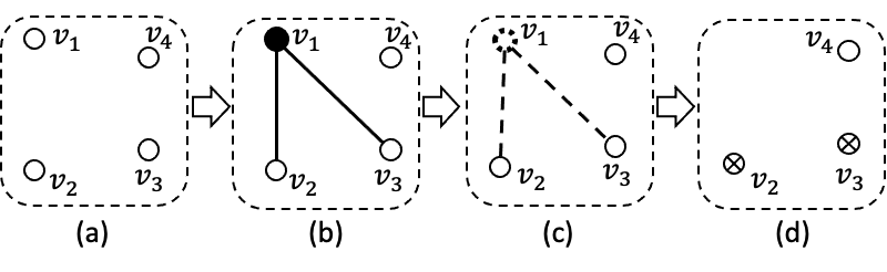
Figure 1: A sampling step for an undirected graph with no isolated vertices: (a) begins with an initial graph that has no edges, and in the more general sampling problem, $V_{\forall}=V_{\exists}=\{v_{1},v_{2},v_{3},v_{4}\}$; (b) sample edges for the vertex $v_{1}$; (c) remove the vertex $v_{1}$ with its sampled edges; (d) and obtain a graph with some vertices already non-isolated ($v_{2}$ and $v_{3}$), resulting in a new sampling problem with $V_{\forall}^{\prime}=\{v_{2},v_{3},v_{4}\}$ and $V_{\exists}^{\prime}=\{v_{4}\}$.

We first show that if $\mathcal{A}_{t}$ is valid w.r.t. $({\widehat{\Gamma}}_{G},V_{\forall})$, the new WFOMS can be reduced to the general WFOMS but with the smaller domain $V_{\forall}^{\prime}=V_{\forall}\setminus\{v_{t}\}$ and

$$V_{\exists}^{\prime}=V_{\exists}\setminus\left(\{v_{t}\}\cup\{v_{i}\mid v_{i}\in V_{\exists}:\pi_{t,i}=\pi^{2}\}\right).$$

The set $V_{\exists}^{\prime}$ removes the vertices that become non-isolated after the sampling of $\mathcal{A}_{t}$ from $V_{\exists}$. It is easy to check that the reduction is sound, because every model of the WFOMS $(\Gamma_{GT}\land\bigwedge_{v\in V_{\exists}^{\prime}}Z(v),V_{\forall}^{\prime},w,\bar{w})$ can be mapped to a unique model of the WFOMS $({\widehat{\Gamma}}_{G}\land\mathcal{A}_{t},V_{\forall},w,\bar{w})$, and vice versa, without affecting the satisfaction and weight of the models.

By the reduction above, the decomposition of (8) can be performed recursively on the WFOMS of ${\widehat{\Gamma}}_{G}$ over $V_{\forall}$. Specifically, the recursive algorithm takes $V_{\forall}$ and $V_{\exists}$ as input,

1. selects a vertex $v_{t}$ from $V_{\forall}$,

2. samples its substructure $\mathcal{A}_{t}$ according to the probability $\mathbb{P}[\mathcal{A}_{t}\mid{\widehat{\Gamma}}_{G}]$, and

3. obtains a new problem with updated $V_{\forall}^{\prime}$ and $V_{\exists}^{\prime}$ for recursion.

The recursion terminates when all substructures $\mathcal{A}_{i}$ are sampled (i.e., $V_{\forall}$ contains a single vertex), or the problem degenerates to a WFOMS on $\mathbf{UFO}^{2}$ sentence (i.e., $V_{\exists}$ is empty). The number of recursions is less than $|V|$, the total number of vertices. An example of a recursive step is shown in Figure 1.

The remaining problem is to sample the substructure $\mathcal{A}_{t}$ according to $\mathbb{P}[\mathcal{A}_{t}\mid{\widehat{\Gamma}}_{G}]$. Recall that $\mathcal{A}_{t}$ determines the edges between $v_{t}$ and vertices in $V_{\forall}^{\prime}$. Let $V_{1}=V_{\forall}^{\prime}\setminus V_{\exists}$ and $V_{2}=V_{\forall}^{\prime}\setminus V_{1}$. We can effectively generate a sample of $\mathcal{A}_{t}$ by sampling two binary partitions of $V_{1}$ and $V_{2}$, respectively, yielding the sets ${V_{11},V_{12}}$ and ${V_{21},V_{22}}$; the vertices in $V_{11}$ and $V_{21}$ will be connected to $v_{t}$, while the vertices in $V_{12}$ and $V_{22}$ will be disconnected to $v_{t}$. It can be demonstrated that the sampling probability of a substructure $\mathcal{A}_{t}$ only depends on the two partition configurations $(|V_{11}|,|V_{12}|)$ and $(|V_{21}|,|V_{22}|)$. The proof of this claim can be found in Section 5.2.4, where the more general case of $\mathbf{FO}^{2}$ sampling is addressed. As a result, the sampling of $\mathcal{A}_{t}$ can be achieved by first sampling the two partition configurations, followed by two random partitions on $V_{1}$ and $V_{2}$ with the respective sampled configurations. To sample a tuple of partition configurations, we utilize the enumerative sampling method. The number of all possible tuples of partition configurations is clearly polynomial in $|V_{\forall}^{\prime}|$, and it will be shown in Section 5.2.4 that the sampling probability of each configurations tuple can be computed in time polynomial in $|V_{\forall}^{\prime}|$. Therefore, the complexity of the sampling algorithm is polynomial in the number of vertices. This, together with the complexity of the recursion procedure, which is also polynomial in the number of vertices, implies that the whole sampling algorithm is lifted.

5.2 Domain Recursive Sampling for 2-tables

We now present our algorithm for sampling 2-tables, which uses the technique illustrated in the previous subsection. The core idea, called domain recursion, involves considering individual objects from the domain at a time, sampling their corresponding atomic facts, and subsequently obtaining a new sampling problem that has a similar form to the original one but with a smaller domain and potentially fewer existentially-quantified formulas. This process is repeated recursively on the reduced sampling problems until the domain has become a singleton or all the existentially-quantified formulas have been eliminated.

Let us consider the WFOMS with fixed 1-types $(\Gamma\land\bigwedge_{i\in[n]}\tau_{i}(e_{i}),\Delta,w,\bar{w})$, where $\Gamma$ is a sentence in SNF (7), $\Delta=\{e_{i}\}_{i\in[m]}$ is a domain of size $n$, and each $\tau_{i}$ is the sampled 1-type of the element $e_{i}$. W.l.o.g. , we suppose that each formula $\varphi_{k}(x,y)$ in the SNF sentence (7) is an atomic formula $R_{k}(x,y)$, where each $R_{k}$ is a binary predicate with weights $w(R_{k})=\bar{w}(R_{k})=1$.

5.2.1 A More General Sampling Problem

We first construct the following sentence from $\Gamma$:

$$\Gamma_{T}:=\forall x\forall y:\psi(x,y)\land\bigwedge_{k\in[m]}\forall x:Z_{k}(x)\Leftrightarrow(\exists y:R_{k}(x,y)),$$ (9)

where each $Z_{k}/1$ is a Tseitin predicate with the weight $w(Z_{k})=\bar{w}(Z_{k})=1$. Note that in (9), the interpretation of $R_{k}$ fully determines the interpretation of $Z_{k}$. Once the 2-tables are sampled, the interpretation of $Z_{k}$ is also fixed, adding no additional cost to the sampling problem. Therefore, for ease of presentation, we will omit the handling of $Z_{k}$ in the following discussion.

We then consider a more general WFOMS problem of the following sentence

$$\Gamma_{T}\land\bigwedge_{i\in[n]}\left(\tau_{i}(e_{i})\land\mathcal{C}_{i}\right)$$ (10)

over a domain of $\{e_{i}\}_{i\in[n]}$, where each $\mathcal{C}_{i}$ is a conjunction over a subset of the ground atoms $\{Z_{k}(e_{i})\}_{k\in[m]}$. We call $\mathcal{C}_{i}$ the existential constraint on the element $e_{i}$ and allow $\mathcal{C}_{i}=\top$, which means $e_{i}$ is not existentially quantified.

The more general sampling problem has the necessary structure for the domain recursion algorithm to be performed. To verify it, the original WFOMS of $\Gamma\land_{i\in[n]}\tau_{i}(e_{i})$ can be reduced to the more general problem by setting all existential constraints to be $\bigwedge_{k\in[m]}Z_{k}(x)$. On the other hand, the WFOMS on the $\mathbf{UFO}^{2}$ sentence $\forall x\forall y:\psi(x,y)\land\bigwedge_{i\in[n]}\tau_{i}(e_{i})$ is also reducible to the problem with $\mathcal{C}_{i}=\top$ for all $i\in[n]$. It is easy to check that these two reductions are both sound.

5.2.2 Block and Cell Types

It is worth noting that the Tseitin predicates $Z_{k}$ introduced in the more general sampling problem are not contained in the given 1-types $\tau_{i}$. Therefore, in order to incorporate these predicates into the sampling problem, we introduce the notions of block and cell types.

Consider a set of Tseitin predicates $\{Z_{k}\}_{k\in[m]}$. A block type $\beta$ is a subset of the atoms $\{Z_{k}(x)\}_{k\in[m]}$. The number of the block types is $2^{m}$, where $m$ is the number of existentially-quantified formulas. We often represent a block type as $\beta(x)$ and view it as a conjunctive formula over the atoms within the block. It is important to note that the block types only indicate which Tseitin atoms should hold for a given element, while the Tseitin atoms not covered by the block types are left unspecified. In contrast, the 1-types explicitly determine the truth values of all unary and reflexive atoms, excluding the Tseitin atoms.

The block type and 1-type work together to define the cell type. A cell type $\eta=(\beta,\tau)$ is a pair of a block type $\beta$ and a 1-type $\tau$. We also write a cell type as a conjunctive formula of $\eta(x)=\beta(x)\land\tau(x)$. The cell type of an element is simply the tuple of its block type (given by the sentence ${\widehat{\Gamma}}$) and 1-type (already sampled in the first stage of the algorithm). The cell types of elements naturally produce a partition of the domain, similar to how a 1-types assignment divides a domain into disjoint subsets. Each disjoint subset of elements is called a cell. The cell configuration is defined as the configuration of the corresponding partition.

With the notion of block and cell type, we can write the existential constraint $\mathcal{C}_{i}$ in (10) as $\beta_{i}(e_{i})$, where $\beta_{i}$ is the block type of the element $e_{i}$, and the sentence (10) as $\Gamma_{T}\land\bigwedge_{i\in[n]}\eta_{i}(e_{i})$, where $\eta_{i}=(\beta_{i},\tau_{i})$.

5.2.3 Domain Recursion

We now show how to apply the domain recursion scheme to the WFOMS $(\Gamma_{T}\land\bigwedge_{i\in[n]}\eta_{i}(e_{i}),\Delta,w,\bar{w})$. Let $\mathcal{A}_{i}$ be the set of ground 2-tables concerning the element $e_{i}$:

$$\mathcal{A}_{i}:=\bigcup_{j\in[n]:j\neq i}\pi_{i,j}(e_{i},e_{j}).$$ (11)

By the domain recursion, we select an arbitrary element $e_{t}$ from $\Delta$ and decompose the sampling probability of a structure $\mathcal{A}$ into

$$\mathbb{P}\left[\mathcal{A}\mid\Gamma_{T}\land\bigwedge_{i\in[n]}\eta_{i}(e_{i})\land\mathcal{A}_{t}\right]\cdot\mathbb{P}\left[\mathcal{A}_{t}\mid\Gamma_{T}\land\bigwedge_{i\in[n]}\eta_{i}(e_{i})\right].$$

We always assume that the substrcture $\mathcal{A}_{t}$ is valid w.r.t. $(\Gamma_{T}\land\bigwedge_{i\in[n]}\eta_{i}(e_{i}),\Delta)$, i.e., $\Gamma_{T}\land\bigwedge_{i\in[n]}\eta_{i}(e_{i})\land\mathcal{A}_{t}$ is satisfiable, or the sampling probability of $\mathcal{A}_{t}$ is zero. We will demonstrate that the WFOMS specified by the first probability in the above equation can be reduced to a new WFOMS of the same form as the original sampling problem, but over a smaller domain $\Delta^{\prime}=\Delta\setminus{e_{t}}$.

We first introduce the notion of relaxed block. Given a 2-table $\pi$ and a block type $\beta$, the relaxed block of $\beta$ under $\pi$ is defined as

$${\beta}\downarrow{{\pi}}:=\beta\setminus\{Z_{k}(x)\mid k\in[m]:R_{k}(y,x)\in\pi\}.$$

Similarly, we can apply the relaxation under $\pi$ on a cell type $\eta=(\beta,\tau)$, resulting in a relaxed cell type ${\eta}\downarrow{{\pi}}=({\beta}\downarrow{{\pi}},\tau)$.

Example 6.

Consider a WFOMS on the sentence

$$\forall x :(Z_{1}(x)\Leftrightarrow(\exists y:R_{1}(x,y))\land$$

$$\forall x :(Z_{2}(x)\Leftrightarrow(\exists y:R_{2}(x,y))$$

$$\land \dots\land Z_{1}(a)\land Z_{2}(a)\land\dots,$$

where only the block type $\beta=\{Z_{1}(x),Z_{2}(x)\}$ of the element $a$ is shown. Suppose the sampled 2-table of $(e_{t},a)$ is

$$\pi=\{\neg R_{1}(x,y),R_{1}(y,x),R_{2}(x,y),\neg R_{2}(y,x)\}.$$

Then the relaxed block of the element $a$ is ${\beta}\downarrow{{\pi}}=\{Z_{2}(x)\}$, as the corresponding quantified formula $\exists y:R_{1}(a,y)$ of $Z_{1}(a)$ is satisfied the fact $R_{1}(a,e_{t})$ in $\pi(e_{t},a)$.

Let

$${\widetilde{\Gamma}}:=\Gamma_{T}\land\bigwedge_{i\in[n]}\eta_{i}(e_{i})\land\mathcal{A}_{t},$$ (12)

and

$${\widetilde{\Gamma}}^{\prime}:=\Gamma_{T}\land\bigwedge_{i\in[n]\setminus\{t\}}({\eta_{i}}\downarrow{{\pi_{t,i}}})(e_{i}).$$ (13)

We have the following lemma.

Lemma 2.

If ${\widetilde{\Gamma}}$ is satisfiable, the reduction from the WFOMS of $({\widetilde{\Gamma}},\Delta,w,\bar{w})$ to $({\widetilde{\Gamma}}^{\prime},\Delta^{\prime},w,\bar{w})$ is sound.

Proof.

We prove the soundness of the reduction by constructing a mapping function from models of ${\widetilde{\Gamma}}^{\prime}$ to models of ${\widetilde{\Gamma}}$. This function is defined as $f(\mu^{\prime})=\mu^{\prime}\cup\mathcal{A}_{t}\cup\tau_{t}(e_{t})$. The function $f$ is clearly deterministic, polynomial-time. To simplify the remaining arguments of the proof, we will first show that $f$ is bijective. Write the sentence ${\widetilde{\Gamma}}$ and ${\widetilde{\Gamma}}^{\prime}$ as

$${\widetilde{\Gamma}}=\forall x\forall y:\psi(x,y)\land\bigwedge_{i\in[n]}\left(\tau_{i}(e_{i})\land\beta_{i}(e_{i})\right)\land\mathcal{A}_{t}\land\Lambda,$$

$${\widetilde{\Gamma}}^{\prime}=\forall x\forall y:\psi(x,y)\land\bigwedge_{i\in[n]\setminus\{t\}}\left(\tau_{i}(e_{i})\land({\beta_{i}}\downarrow{{\pi_{t,i}}})(e_{i})\right)\land\Lambda,$$

where $\Lambda=\bigwedge_{k\in[m]}\forall:Z_{k}(x)\Leftrightarrow(\exists y:R_{k}(x,y))$.

($\Rightarrow$)

For any model $\mu^{\prime}$ in $\mathcal{M}_{{\widetilde{\Gamma}}^{\prime},\Delta^{\prime}}$, we will prove that $f(\mu^{\prime})=\mu^{\prime}\cup\mathcal{A}_{t}\cup\tau_{t}(e_{t})$ is a model in $\mathcal{M}_{{\widetilde{\Gamma}},\Delta}$. First, one can easily check that $f(\mu^{\prime})$ satisfies $\forall x\forall y:\psi(x,y)\land\bigwedge_{i\in[n]}\tau_{i}(e_{i})$. Next, we will demonstrate that $f(\mu^{\prime})$ also satisfies $\bigwedge_{i\in[n]}\beta_{i}(e_{i})\land\Lambda$. For any element $i\in[n]\setminus\{t\}$, we have that $\exists y:R_{k}(e_{i},y)$ is true in $\mu^{\prime}$ (and also $f(\mu^{\prime})$) for all $k\in[m]$ such that $Z_{k}(x)\in{\beta_{i}}\downarrow{{\pi_{t,i}}}$. By the definition of the relaxed block, for any $k\in[m]$ such that $Z_{k}(x)\in\beta_{i}\setminus({\beta_{i}}\downarrow{{\pi_{t,i}}})$, the ground relation $R_{k}(e_{i},e_{t})$ is in $\mathcal{A}_{t}$, and thus $\exists y:R_{k}(e_{i},y)$ is also satisfied in $f(\mu^{\prime})$. It follows that $\exists y:R_{k}(e_{i},y)$ is true in $f(\mu^{\prime})$ for all $k\in[m]$ such that $Z_{k}(x)\in\beta_{i}$. Furthermore, the satisfaction of $\exists y:R_{k}(e_{t},y)$ for all $k\in[m]$ such that $Z_{k}(x)\in\beta_{t}$ is guaranteed by the satisfiability of ${\widetilde{\Gamma}}$. Therefore, it is easy to show that $f(\mu^{\prime})$ satisfies $\bigwedge_{i\in[n]}\beta_{i}(e_{i})\land\Lambda$, which together with the satisfaction of $\forall x\forall y:\psi(x,y)\land\bigwedge_{i\in[n]}\tau_{i}(e_{i})$ implies that $f(\mu^{\prime})$ is a model of ${\widetilde{\Gamma}}$.

($\Leftarrow$)

For any model $\mu$ in $\mathcal{M}_{{\widetilde{\Gamma}},\Delta}$, we will show that there exists a unique model $\mu^{\prime}$ in $\mathcal{M}_{{\widetilde{\Gamma}}^{\prime},\Delta^{\prime}}$ such that $f(\mu^{\prime})=\mu$. Let the respective structure be $\mu^{\prime}=\mu\setminus((\mathcal{A}_{t})\cup\tau_{t}(e_{t}))$, and the uniqueness is is clear from the definition of $f$. First, it is easy to check that $\mu^{\prime}$ satisfies $\forall x\forall y:\psi(x,y)\land\bigwedge_{i\in[n]\setminus\{t\}}\tau_{i}(e_{i})$. Then we will show that $\mu^{\prime}$ also satisfies $\bigwedge_{i\in[n]\setminus\{t\}}({\beta_{i}}\downarrow{{\pi_{t,i}}})(e_{i})\land\Lambda$. For any $i\in[n]\setminus\{t\}$, we have that $\exists y:R_{k}(e_{i},e)$ is true in $\mu$. Grounding $\exists y:R_{k}(e_{i},e)$ over $\Delta$ and replacing the atoms $R_{k}(e_{t},e_{j})$ with their truth values in $\mathcal{A}_{t}$, we have that $\bigvee_{j\in[n]\setminus\{t\}}R_{k}(e_{i},e_{j})$ is true in $\mu^{\prime}$ for all $k\in[m]$ such that $Z_{k}(x)\in{\beta_{i}}\downarrow{{\pi_{t,i}}}$. Thus, $\mu^{\prime}$ also satisfies $\bigwedge_{i\in[n]\setminus\{t\}}({\beta_{i}}\downarrow{{\pi_{t,i}}})(e_{i})\land\Lambda$. This, along with the satisfaction of $\forall x\forall y:\psi(x,y)\land\bigwedge_{i\in[n]\setminus\{t\}}\tau_{i}(e_{i})$, leads to the conclusion.

Now, we are prepared to demonstrate the consistency of sampling probability through the mapping function. Since $f$ is bijective, it is sufficient to show

$$\mathbb{P}[f(\mu^{\prime})\mid{\widetilde{\Gamma}};\Delta,w,\bar{w}]=\mathbb{P}[\mu^{\prime}\mid{\widetilde{\Gamma}}^{\prime};\Delta^{\prime},w,\bar{w}]$$

for any model in $\mathcal{M}_{{\widetilde{\Gamma}}^{\prime},\Delta^{\prime}}$. By the definition of the mapping function $f$, we have

$$\langle w,\bar{w}\rangle(f(\mu^{\prime}))=\langle w,\bar{w}\rangle(\mu^{\prime})\cdot\langle w,\bar{w}\rangle(\mathcal{A}_{t})\cdot\langle w,\bar{w}\rangle(\tau_{t}).$$

Moreover, due to the bijectivity of $f$, we have

$$\mathsf{WFOMC}({\widetilde{\Gamma}},\Delta,w,\bar{w}) =\sum_{\mu\in\mathcal{M}_{{\widetilde{\Gamma}},\Delta}}\langle w,\bar{w}\rangle(\mu)$$ (14)

$$=\sum_{\mu^{\prime}\in\mathcal{M}_{{\widetilde{\Gamma}}^{\prime},\Delta^{\prime}}}\langle w,\bar{w}\rangle(f(\mu^{\prime}))$$

$$=\langle w,\bar{w}\rangle(\mathcal{A}_{t})\cdot\langle w,\bar{w}\rangle(\tau_{t})\cdot\sum_{\mu^{\prime}\in\mathcal{M}_{{\widetilde{\Gamma}}^{\prime},\Delta^{\prime}}}\langle w,\bar{w}\rangle(\mu^{\prime})$$

$$=\langle w,\bar{w}\rangle(\mathcal{A}_{t})\cdot\langle w,\bar{w}\rangle(\tau_{t})\cdot\mathsf{WFOMC}({\widetilde{\Gamma}}^{\prime},\Delta^{\prime},w,\bar{w}).$$

Finally, by the definition of conditional probability, we can write

$$\mathbb{P}[f(\mu^{\prime})\mid{\widetilde{\Gamma}};\Delta,w,\bar{w}] =\frac{\langle w,\bar{w}\rangle(f(\mu^{\prime}))}{\mathsf{WFOMC}({\widetilde{\Gamma}},\Delta,w,\bar{w})}$$ (15)

$$=\frac{\langle w,\bar{w}\rangle(\mu^{\prime})\cdot\langle w,\bar{w}\rangle(\mathcal{A}_{t})\cdot\langle w,\bar{w}\rangle(\tau_{t})}{\langle w,\bar{w}\rangle(\mathcal{A}_{t})\cdot\langle w,\bar{w}\rangle(\tau_{t})\cdot\mathsf{WFOMC}({\widetilde{\Gamma}}^{\prime},\Delta^{\prime},w,\bar{w})}$$

$$=\frac{\langle w,\bar{w}\rangle(\mu^{\prime})}{\mathsf{WFOMC}({\widetilde{\Gamma}}^{\prime},\Delta^{\prime},w,\bar{w})}$$

$$=\mathbb{P}[\mu^{\prime}\mid{\widetilde{\Gamma}}^{\prime};\Delta^{\prime},w,\bar{w}],$$

completing the proof. ∎

With the sound reduction presented above, one can readily perform the domain recursion on the more general WFOMS problem. The only remaining task is the sampling of the substructure $\mathcal{A}_{t}$ at each recursive step, which will be discussed in the following subsection.

5.2.4 Sampling substructures

For the sake of brevity, we shall limit our focus to the initial recursive step involving sampling $\mathcal{A}_{t}$ from $\Gamma_{T}\land\bigwedge_{i\in[n]}\eta_{i}(e_{i})$. The subsequent steps can be executed by the same process.

We will follow a similar approach as in the 1-types sampling, which samples $\mathcal{A}_{t}$ through random partitions on cells. Let $N_{c}$ be the total number of cell types, and fix the linear order of cell types as $\eta^{1},\eta^{2},\dots,\eta^{N_{c}}$. For all $i\in[N_{c}]$, denote by $C_{\eta^{i}}\subseteq\Delta^{\prime}$ the cells of $\eta^{i}$ constructed from the cell types $\eta_{1},\eta_{2},\dots,\eta_{n-1}$:

$$C_{\eta^{i}}:=\{e_{j}\mid j\in[n-1]:\eta_{j}=\eta^{i}\}.$$

Let $N_{b}$ be the number of all 2-tables, and fix the linear order of 2-tables as $\pi^{1},\pi^{2},\dots,\pi^{N_{b}}$. Recall that $\mathcal{A}_{t}$ consists of the ground 2-tables of all tuples of $e_{t}$ and the elements in $\Delta^{\prime}$. Any substructure $\mathcal{A}_{t}$ can be represented as a collection of $N_{c}$ partitions; each partition is applied to a cell $C_{\eta^{i}}$ in order to split it into $N_{b}$ disjoint subsets; each of these subsets is associated with a specific 2-table $\pi^{j}$, and contains precisely the elements $e$, whose combination $(e_{t},e)$ with $e_{t}$ has the 2-table $\pi^{j}$.

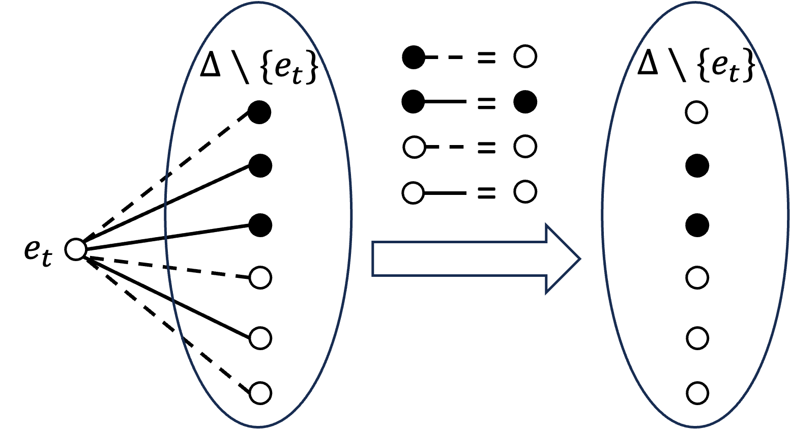
Figure 2: An example of sampling a substructure. There are two cell types, denoted by and , and two 2-tables, denoted by and . The sampled substructure $\mathcal{A}_{t}$ is represented on the left, whose 2-tables configuration is $(g_{\text{\faCircle{}},\text{ \leavevmode\hbox to16.16pt{\vbox to0.8pt{\text{[drawing]}}}{}}}^{\mathcal{A}_{t}},g_{\text{\faCircle{}},\text{ \leavevmode\hbox to15.03pt{\vbox to0.8pt{\text{[drawing]}}}{}}}^{\mathcal{A}_{t}},g_{\text{\faCircleThin{}},\text{ \leavevmode\hbox to16.16pt{\vbox to0.8pt{\text{[drawing]}}}{}}}^{\mathcal{A}_{t}},g_{\text{\faCircleThin{}},\text{ \leavevmode\hbox to15.03pt{\vbox to0.8pt{\text{[drawing]}}}{}}}^{\mathcal{A}_{t}})=(1,2,2,1)$. With the relaxations of cell types defined above the arrow, where, e.g., $\text{\faCircle{}}\text{ \leavevmode\hbox to16.16pt{\vbox to0.8pt{\text{[drawing]}}}}=\text{\faCircleThin{}}$ means the relaxed cell type of under is , the reduced cell types for each element is presented on the right. One can easily obtain the reduced cell configuration from the 2-table configuration $(g_{\text{\faCircle{}},\text{ \leavevmode\hbox to16.16pt{\vbox to0.8pt{\text{[drawing]}}}{}}}^{\mathcal{A}_{t}},g_{\text{\faCircle{}},\text{ \leavevmode\hbox to15.03pt{\vbox to0.8pt{\text{[drawing]}}}{}}}^{\mathcal{A}_{t}},g_{\text{\faCircleThin{}},\text{ \leavevmode\hbox to16.16pt{\vbox to0.8pt{\text{[drawing]}}}{}}}^{\mathcal{A}_{t}},g_{\text{\faCircleThin{}},\text{ \leavevmode\hbox to15.03pt{\vbox to0.8pt{\text{[drawing]}}}{}}}^{\mathcal{A}_{t}})$.

Consider a substructure $\mathcal{A}_{t}$ and its corresponding partitions. For any cell $C_{\eta^{i}}$, let $g_{\eta^{i},\pi^{j}}^{\mathcal{A}_{t}}$ represents the cardinality of the subset in $C_{\eta^{i}}$ associated with the 2-table $\pi^{j}$. We can write the configuration of the partition of cell $C_{\eta^{i}}$ as $(g_{\eta^{i},\pi^{j}}^{\mathcal{A}_{t}})_{j\in[N_{b}]}$, and denote it by the vector $\mathbf{g}_{\eta^{i}}^{\mathcal{A}_{t}}$. The 2-tables configuration $\mathbf{g}$ of $\mathcal{A}_{t}$ is then defined as the concatenation of partition configurations over all cells, i.e., $\mathbf{g}^{\mathcal{A}_{t}}:=\bigoplus_{i\in[N_{c}]}\mathbf{g}_{\eta^{i}}^{\mathcal{A}_{t}}$, where $\oplus$ denotes the concatenation operator. Figure 2 illustrates an example of a substructure and its 2-tables configuration. In the following, we will show that the sampling probability of $\mathcal{A}_{t}$ is entirely determined by its corresponding 2-tables configuration.

To begin, it is clear that the sampling probability of $\mathcal{A}_{t}$ is proportional to the value of $\mathsf{WFOMC}(\Gamma_{T}\land\bigwedge_{i\in[n]}\eta_{i}(e_{i})\land\mathcal{A}_{t},\Delta,w,\bar{w})$. As stated by (14), we can write this WFOMC as

$$\mathsf{WFOMC}({\widetilde{\Gamma}}^{\prime},\Delta^{\prime},w,\bar{w})\cdot\langle w,\bar{w}\rangle(\tau_{t})\cdot\langle w,\bar{w}\rangle(\mathcal{A}_{t})$$ (16)

where ${\widetilde{\Gamma}}^{\prime}=\Gamma_{T}\land\bigwedge_{i\in[n]\setminus\{t\}}({\eta_{i}}\downarrow{{\pi_{t,i}}})(e_{i})$ is the reduced sentence given the substrcture $\mathcal{A}_{t}$. Denote by $\mathbf{w}=\left(\langle w,\bar{w}\rangle(\pi^{i})\right)_{i\in N_{b}}$, the weight vector of 2-tables. We can write (16) as

$$\mathsf{WFOMC}({\widetilde{\Gamma}}^{\prime},\Delta^{\prime},w,\bar{w})\cdot\langle w,\bar{w}\rangle(\tau_{t})\cdot\prod_{i\in[N_{c}]}\mathbf{w}^{\mathbf{g}_{\eta^{i}}^{\mathcal{A}_{t}}}.$$ (17)

In the equation above, the 1-types $\tau_{t}$ is fixed, and the last term fully depends on the 2-tables configurations $\mathbf{g}^{\mathcal{A}_{t}}$. The only part that needs further analysis is the WFOMC of ${\widetilde{\Gamma}}^{\prime}$.

The WFOMC of ${\widetilde{\Gamma}}^{\prime}$ can be viewed as the WFOMC of $\Gamma_{T}$ conditioned on the cell types ${\eta_{i}}\downarrow{{\pi_{t,i}}}$. By the symmetry of the weighting function, its value does not depend on the specific cell types ${\eta_{i}}\downarrow{{\pi_{t,i}}}$ assigned to each element, but instead relies on the overall cell configuration corresponding to the cell types ${\eta_{i}}\downarrow{{\pi_{t,i}}}$. We denote this cell configuration by a vector $(n_{\eta^{i}})_{i\in[N_{c}]}$, where $n_{\eta^{i}}$ represents the number of elements whose cell type is $\eta^{i}$ under the relaxation of 2-tables in $\mathcal{A}_{t}$. By the definition of $g_{\eta^{i},\pi^{j}}^{\mathcal{A}_{t}}$, which is the number of elements in the cell $C_{\eta^{i}}$ that are relaxed by the 2-table $\pi^{j}$, we can write each $n_{\eta^{i}}$ as

$$n_{\eta^{i}}=\sum_{j\in[N_{c}]}\sum_{k\in[N_{b}]:{\eta^{j}}\downarrow{{\pi^{k}}}=\eta^{i}}g_{\eta^{j},\pi^{k}}^{\mathcal{A}_{t}}.$$ (18)

For the example in Figure 2, we have $n_{\text{\faCircle{}}}=g_{\text{\faCircle{}},\text{ \leavevmode\hbox to15.03pt{\vbox to0.8pt{\text{[drawing]}}}{}}}^{\mathcal{A}_{t}}$ and $n_{\text{\faCircleThin{}}}=g_{\text{\faCircle{}},\text{ \leavevmode\hbox to16.16pt{\vbox to0.8pt{\text{[drawing]}}}{}}}^{\mathcal{A}_{t}}+g_{\text{\faCircleThin{}},\text{ \leavevmode\hbox to16.16pt{\vbox to0.8pt{\text{[drawing]}}}{}}}^{\mathcal{A}_{t}}+g_{\text{\faCircleThin{}},\text{ \leavevmode\hbox to15.03pt{\vbox to0.8pt{\text{[drawing]}}}{}}}^{\mathcal{A}_{t}}$. Therefore, we have that the 2-tables configuration fully determines the cell configuration and, consequently, the WFOMC of ${\widetilde{\Gamma}}^{\prime}$.

According to the aforementioned reasoning, the sampling probability of a substructure is completely determined by its 2-tables configuration. Thus, we can adopt a similar approach to the one we used to sample 1-types in Section 4.1 and sample $\mathcal{A}_{t}$ by first sampling a 2-tables configuration, and then randomly partitioning the cells accordingly. The sampling for the 2-tables configuration can be achieved by the enumerative sampling method. For any 2-tables configuration $\mathbf{g}^{\mathcal{A}_{t}}$, its sampling probability is proportional to the value of (17) multiplied by $\prod_{i\in[N_{c}]}\binom{|C_{\eta^{i}}|}{\mathbf{g}_{\eta^{i}}^{\mathcal{A}_{t}}}$, where $|C_{\eta^{i}}|$ is the cardinality of $C_{\eta^{i}}$.

Finally, we need to ensure that the sampled substructure $\mathcal{A}_{t}$ is valid w.r.t. $(\Gamma_{T}\land\bigwedge_{i\in[n]}\eta_{i}(e_{i}),\Delta)$. It can be easily achieved by imposing some constraints on the 2-tables configuration to be sampled. A 2-table $\pi$ is called coherent with a 1-types tuple $(\tau,\tau^{\prime})$ if, for some domain elements $a$ and $b$, the interpretation of $\tau(a)\cup\pi(a,b)\cup\tau^{\prime}(b)$ satisfies the formula $\psi(a,b)\land\psi(b,a)$. The following two constraints on the 2-tables configuration can make the sampled substructure valid:

• Any 2-table $\pi_{t,i}$ contained in $\mathcal{A}_{t}$ must be coherent with $\tau_{t}$ and $\tau_{i}$, the 1-types of $e_{t}$ and $e_{i}$. This translates to a requirement on the 2-tables configuration that when sampling a configuration of partition of a cell $C_{\eta^{i}}$, the cardinality of 2-tables that are not coherent with $\tau_{t}$ and $\tau_{i}$ is restricted to be $0$;

• For any Tseitin $Z_{k}$ in the block type $\beta_{t}$, the substructure $\mathcal{A}_{t}$ must contain at least one ground atom $R_{k}(e_{t},a)$, where $a$ is a domain element, to make $\mathcal{A}_{t}$ satisfy the existentially quantified formula $\exists y:R_{k}(e_{t},y)$. This means that there must be at least one 2-table $\pi$ such that $R_{k}(x,y)\in\pi$, whose cardinality in some cells is nonzero.

5.2.5 Sampling Algorithm

Algorithm 1 $\textsf{TwoTablesSampler}(\Gamma_{T},\Delta,w,\bar{w},(\eta_{i})_{i\in[n]})$

1:if $n=1$ then

2:     return $\emptyset$

3:end if

4:if all block types $\beta_{1},\dots,\beta_{n}$ are $\top$ then

5:     return a set of 2-tables sampled by the algorithm in Section 4.2 from $\forall x\forall y:\psi(x,y)\land\bigwedge_{i\in[n]}\tau_{i}(e_{i})$

6:end if

7:$W\leftarrow\mathsf{WFOMC}(\Gamma_{T}\land\bigwedge_{i\in[n]}\eta_{i}(e_{i}),\Delta,w,\bar{w})$

8:Choose $t\in[n]$; $\Delta^{\prime}\leftarrow\Delta\setminus\{e_{t}\}$

9:Obtain the cells $C_{\eta^{1}},\dots,C_{\eta^{N_{c}}}$ given by $\eta_{1},\dots,\eta_{n-1}$

10:for $\left(\mathbf{g}_{\eta^{i}}\right)_{i\in[N_{c}]}\leftarrow\bigotimes_{i\in[N_{c}]}\mathcal{T}_{|C_{\eta^{i}}|,N_{b}}$ do $\triangleright$ $\bigotimes$ is the Cartesian product

11:     $\mathbf{g}\leftarrow\bigoplus_{i\in[N_{c}]}\mathbf{g}_{\eta^{i}}$

12:     if $\textsf{ExSat}\left(\mathbf{g},\eta_{t}\right)$ then

13:         Obtain the reduced cell configuration $(n_{\eta^{i}})_{i\in[N_{c}]}$ from $\mathbf{g}$ by (18)

14:         $W^{\prime}\leftarrow\eqref{eq:structure_weight}\cdot\prod_{i\in[N_{c}]}\binom{n_{\eta^{i}}}{\mathbf{g}_{\eta^{i}}}$

15:         if $\textsf{Uniform}(0,1)<\frac{W^{\prime}}{W}$ then

16:              $\mathbf{g}^{*}\leftarrow\mathbf{g}$

17:              break

18:         else

19:              $W\leftarrow W-W^{\prime}$

20:         end if

21:     end if

22:end for

23:Remove $e_{t}$ from the cell $C_{\eta_{t}}$; $\mathcal{A}\leftarrow\emptyset$

24:for $i\in[N_{c}]$ do

25:     Randomly partition the cell $C_{\eta^{i}}$ into $\left\{G_{\eta^{i},\pi^{j}}\right\}_{j\in[N_{b}]}$ according to $\mathbf{g}^{*}_{\eta^{i}}$

26:     for $j\in[N_{b}]$ do

27:         $\mathcal{A}\leftarrow\mathcal{A}\cup\left\{\pi^{j}(e_{t},e)\right\}_{e\in G_{\eta^{i},\pi^{j}}}$

28:         $\forall e_{s}\in G_{\eta^{i},\pi^{j}},\eta_{s}^{\prime}\leftarrow{\eta_{s}}\downarrow{{\pi^{j}}}$

29:     end for

30:end for

31:$\mathcal{A}\leftarrow\mathcal{A}\cup\textsf{TwoTablesSampler}(\Gamma_{T},\Delta^{\prime},w,\bar{w},\left(\eta_{i}^{\prime}\right)_{i\in[n-1]})$

32:return $\mathcal{A}$

By combining all the ingredients discussed above, we now present our sampling algorithm for 2-tables, as shown in Algorithm 1. The overall structure of the algorithm follows a recursive approach, where a recursive call with a smaller domain and relaxed cell types is invoked at Line 31. The algorithm terminates when the input domain contains a single element (at Line 1) or there are no existential constraints on the elements (at Line 4). In the latter case, the algorithm resorts to the 2-tables sampling algorithm for $\mathbf{UFO}^{2}$ presented in Section 4.2. In Lines 10-22, all possible 2-tables configurations are enumerated. For each configuration, we compute its corresponding weight in Lines 13-14 and decide whether it should be sampled in Lines 15-20, where $\textsf{Uniform}(0,1)$ is a random number uniformly distributed in $[0,1]$. When the 2-tables configuration has been sampled, we randomly partition the cells, and then update the sampled 2-tables and the cell type of each element respectively at Line 27 and 28. The submodule $\textsf{ExSat}(\mathbf{g},\eta)$ at Line 12 is used to check whether the 2-tables configuration $\mathbf{g}$ guarantees the validity of the sampled substructures. Its pseudo-code can be found in D.2.

Lemma 3.

The complexity of $\textsf{TwoTablesSampler}(\cdot,\cdot,\cdot,\cdot)$ in Algorithm 1 is polynomial in the size of the input domain.

Proof.

The algorithm TwoTablesSampler is invoked at most $n$ times, where $n$ is the size of the domain. The main computation of each recursive call is the for-loop, where we need to iterate over all $\prod_{i\in[N_{c}]}|\mathcal{T}_{n_{\eta^{i}},N_{b}}|$ possible configurations. Recall that the size of the configuration space $\mathcal{T}_{M,m}$ is polynomial in $M$. Thus the number of iterations executed by the loop is also polynomial in the domain size. The other complexity arises from the WFOMC problems of $W$ and (17). These problems can be viewed as WFOMC with a set of unary facts, whose size is clearly polynomial in the domain size. Therefore, according to Proposition 1 and the liftability of $\mathbf{FO}^{2}$ for WFOMC, the aforementioned counting problems can be solved in polynomial-time in the domain size. As a result, the complexity of the entire algorithm is polynomial in the size of the input domain. ∎

Remark 2.

We note that there are several optimizations to TwoTablesSampler in our implementation, e.g., heuristically choosing the domain element for recursion so that the algorithm can quickly reach the terminal condition. However, the algorithm as described here is easier to understand and efficient enough to prove our main result, so we leave the discussion of some of the optimizations to D.1.

With the proposed TwoTablesSampler, we can now prove Theorem 2.

Proof of Theorem 2.

By Lemma 1, it is sufficient to demonstrate that all SNF sentences are sampling liftable. To achieve this, we construct a lifted WMS for SNF sentences. The WMS consists of two stages, one for sampling 1-types and the other for 2-tables, in a manner similar to the WMS for $\mathbf{UFO}^{2}$. The sampling of 1-types can be realized using the same methodology in the proof of Theorem 1. Due to the domain-liftability of $\mathbf{FO}^{2}$ for WFOMC, this approach retains its polynomial complexity w.r.t. the domain size. The sampling of 2-tables is handled by TwoTablesSampler, whose complexity has been proved polynomial in the domain size, according to Lemma 3. Therefore, the entire WMS runs in time polynomial in the domain size, and hence is domain-lifted. ∎

6 $\mathbf{C}^{2}$ is Sampling Liftable

In this section, we extend the sampling liftability of $\mathbf{FO}^{2}$ to $\mathbf{C}^{2}$, the 2-variables fragment of first-order logic with counting quantifiers $\exists_{=k}$, $\exists_{\leq k}$ and $\exists_{\geq k}$. These counting quantifiers are defined as follows. Let $\mathcal{A}$ be a structure defined on a domain $\Delta$. Then the sentence $\exists_{=k}x:\varphi(x)$ is true in $\mathcal{A}$ if there are exactly $k$ distinct elements $t_{1},\dots,t_{k}\in\Delta$ such that $\mathcal{A}\models\varphi(t_{i})$. For example, the sentence

$$\forall x\forall y:(E(x,y)\Rightarrow E(y,x))\land\forall x:\neg E(x,x)\land\forall x\exists_{=2}y:E(x,y)$$

encodes 2-regular graphs, i.e., graphs where each vertex has exactly two neighbors. The other two counting quantifiers can be defined: $(\exists_{\leq k}x:\varphi(x))\Leftrightarrow(\forall x:\neg\varphi(x))\land\bigvee_{i\in[k]}(\exists_{=i}x:\varphi(x))$ and $(\exists_{\geq k}x:\varphi(x))\Leftrightarrow\neg(\exists_{\leq k}x:\varphi(x))$. For ease of presentation, we allow the counting parameter $k=0$, and define the quantifier $\exists_{=0}$ by $(\exists_{=0}x:\varphi(x))\Leftrightarrow(\forall x:\neg\varphi(x))$. Note that the existential quantifiers $\exists$ can be always written as $\exists_{\geq 1}$, and thus we omit $\exists$ in the following discussion and assume that $\mathbf{C}^{2}$ is obtained by adding the counting quantifiers to $\mathbf{UFO}^{2}$. The notation of $[\cdot]$ is extended such that $[i,j]$ denotes the set of integers $\{i,i+1,\dots,j\}$.

The sampling liftability and the lifted sampling algorithm for $\mathbf{C}^{2}$ are built upon the framework for $\mathbf{FO}^{2}$ as in Section 5, which includes the following components.

Normal form

We first introduce the following sentence as a normal form of $\mathbf{C}^{2}$:

$$\Gamma_{\forall}\land\bigwedge_{i\in[m]}(\forall x:A_{i}(x)\Leftrightarrow(\exists_{=k_{i}}y:R_{i}(x,y))),$$ (19)

where $\Gamma_{\forall}$ is a $\mathbf{UFO}^{2}$ sentence, each $k_{i}$ is a non-negative integer, $R_{k}(x,y)$ is an atomic formula, and $A_{k}$ is a unary predicate. Any $\mathbf{C}^{2}$ sentence can be converted into this normal form and the corresponding reduction is sound. This process involves converting all $\exists_{\leq k}$ and $\exists_{\geq k}$ quantifiers into $\exists_{=k}$ quantifiers according to the definition of counting quantifiers. Then a similar approach for converting $\mathbf{FO}^{2}$ sentence into SNF in Section 5 is utilized to substitute each $\exists_{=k}y:R_{i}(x,y)$ with an auxiliary atom $A_{i}(x)$. The details can be found in B.2.

Lemma 4.

For any WFOMS of $\mathfrak{S}=(\Gamma,\Delta,w,\bar{w})$ where $\Gamma$ is a $\mathbf{C}^{2}$ sentence, there exists a WFOMS $\mathfrak{S}^{\prime}=(\Gamma^{\prime},\Delta,w^{\prime},\bar{w}^{\prime})$ where $\Gamma^{\prime}$ is of the form (19) and $\max_{k\in[q]}m_{k}\leq|\Delta|$, such that the reduction from $\mathfrak{S}$ to $\mathfrak{S}^{\prime}$ is sound.

Sampling 1-types

The 1-type for each element $e_{i}$ can be sampled by the same approach as in Section 5. Let $\tau_{1},\tau_{2},\dots,\tau_{n}$ be the sampled 1-types. The predicates $A_{i}$ are contained in these 1-types, and thus will be determined after the 1-types sampling.

A more general WFOMS for 2-tables sampling

Similar to the case of $\mathbf{FO}^{2}$, we need to transform the 2-tables sampling problem into a more general form to apply the domain recursion scheme. For each formula $\exists_{=k_{j}}y:R_{j}(x,y)$, we introduce $2(k_{j}+1)$ new unary predicates $Z^{\exists}_{j,0},Z^{\exists}_{j,1},\dots,Z^{\exists}_{j,k_{j}}$, $Z^{\nexists}_{j,0},Z^{\nexists}_{j,1},\dots,Z^{\nexists}_{j,k_{j}}$, and append the conjunction

$$\forall x:\left(Z^{\exists}_{j,q}(x)\Leftrightarrow(\exists_{=q}y:R_{j}(x,y))\right)\land\left(Z^{\nexists}_{j,q}(x)\Leftrightarrow\neg(\exists_{=q}y:R_{j}(x,y))\right)$$

over $q\in[0,k_{j}]$ to $\Gamma_{\forall}$, resulting in a new sentence $\Gamma_{T}$. Let

$$\mathcal{Z}_{j}:=\{Z^{\exists}_{j,0}(x),\dots,Z^{\exists}_{j,k_{j}}(x),Z^{\nexists}_{j,0}(x),\dots,Z^{\nexists}_{j,k_{j}}(x),\top\},$$

and

$$\mathcal{Z}:=\{\{Z_{1}(x),Z_{2}(x),\dots,Z_{m}(x)\}\mid Z_{1}(x)\in\mathcal{Z}_{1},\dots,Z_{m}(x)\in\mathcal{Z}_{m}\}.$$ (20)

The more general WFOMS is then defined on

$$\Gamma_{T}\land\bigwedge_{i\in[n]}\tau_{i}(e_{i})\land\bigwedge_{i\in[n]}\nu_{i}(e_{i}),$$ (21)

where each $\nu_{i}(x)$ is a conjunction over a set of atomic formulas in $\mathcal{Z}$:

$$\nu_{i}(x)\in\left\{\bigwedge_{j\in[m]}Z_{j}(x)\mid\{Z_{1}(x),Z_{2}(x),\dots,Z_{m}(x)\}\in\mathcal{Z}\right\}.$$

Let $w(Z_{j,q}^{*})=\bar{w}(Z_{j,q}^{*})=1$ for all $j\in[m],q\in[0,k_{j}]$ and $*\in\{\exists,\nexists\}$. It is easy to check that the 2-tables sampling problem is reducible to the more general WFOMS, and the reduction is sound.

Example 7.

Consider the WFOMS on the following sentence:

$$\forall x\forall y:(E(x,y)\Rightarrow E(y,x))\land\forall x:\neg E(x,x)\land$$

$$\forall x:Red(x)\Leftrightarrow(\exists_{=2}y:E(x,y)).$$

It encodes the colored graphs where a vertex is colored red if and only if it has exactly two neighbors. Suppose the domain is $\{v_{1},v_{2},v_{3},v_{4}\}$, and the sampled 1-types for each element are $\tau_{1}=\{Red(x)\}$, $\tau_{2}=\{\neg Red(x)\}$, $\tau_{3}=\{\neg Red(x)\}$, $\tau_{4}=\{Red(x)\}$. The transformed sentence for the more general WFOMS is

$$\forall x\forall y:E(x,y)\Rightarrow E(y,x)\land\forall x:\neg E(x,x)\land$$

$$Red(v_{1})\land\neg Red(v_{2})\land Red(v_{3})\land Red(v_{4})\land$$

$$\forall x:(Z^{\exists}_{1,0}(x)\Leftrightarrow(\exists_{=0}y:E(x,y)))\land\forall x:(Z^{\nexists}_{1,0}(x)\Leftrightarrow\neg(\exists_{=0}y:E(x,y)))\land$$

$$\forall x:(Z^{\exists}_{1,1}(x)\Leftrightarrow(\exists_{=1}y:E(x,y)))\land\forall x:(Z^{\nexists}_{1,1}(x)\Leftrightarrow\neg(\exists_{=1}y:E(x,y)))\land$$

$$\forall x:(Z^{\exists}_{1,2}(x)\Leftrightarrow(\exists_{=2}y:E(x,y)))\land\forall x:(Z^{\nexists}_{1,2}(x)\Leftrightarrow\neg(\exists_{=2}y:E(x,y)))\land$$

$$Z_{1,2}^{\exists}(v_{1})\land Z_{1,2}^{\nexists}(v_{2})\land Z_{1,2}^{\nexists}(v_{3})\land Z_{1,2}^{\exists}(v_{4}).$$

The block types for each element are $\nu_{1}(x)=\{Z^{\exists}_{1,2}(x)\}$, $\nu_{2}(x)=\{Z^{\nexists}_{1,2}(x)\}$, $\nu_{3}(x)=\{Z^{\nexists}_{1,2}(x)\}$, $\nu_{4}(x)=\{Z^{\exists}_{1,2}(x)\}$.

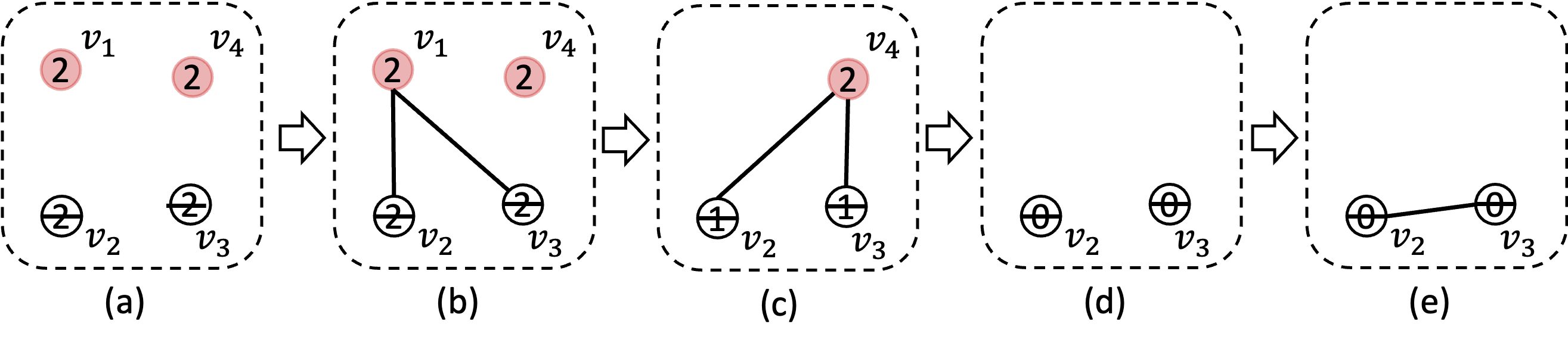
Figure 3: An illustration of domain recursion for the WFOMS in Example 7. The vertices $v_{1}$ and $v_{4}$ are colored red, while the vertices $v_{2}$ and $v_{3}$ are not colored, according to the sampled 1-types. The number shown in each vertex corresponds to its block type, denoting the number of neighbors that the vertex should or should not have, e.g., $v_{1}$ should have exactly two neighbors, while $v_{2}$ should not have any neighbors. In each domain recursion step, the block types of the selected element are relaxed according to the sampled edges. Note that in the final step, the edge between $v_{1}$ and $v_{4}$ is always sampled, as the block type of $v_{1}$ and $v_{3}$ requires them to have at least one neighbor.

Domain recursion

The domain recursion scheme is applicable to the WFOMS of (21), where we view the sets in $\mathcal{Z}(x)$ as “block types”, and $\nu_{i}(x)$ as the block type of $e_{i}$. When the substructure $\mathcal{A}_{t}$ of an element $e_{t}$ has been sampled, the block types of the remaining elements are relaxed by the 2-tables in $\mathcal{A}_{t}$. This will lead to a new WFOMS problem on the sentence in the same form of (21), but with a smaller domain. We can show that this reduction to the new WFOMS problem is sound. The argument is similar to what we have done for $\mathbf{FO}^{2}$, and is deferred to F. An example of this reduction is illustrated in Figure 3.

Lemma 5.

Define the relaxed block type ${\nu}\downarrow{{\pi}}$ of a block type $\nu$ under a 2-table $\pi$ as a set in $\mathcal{Z}$ such that for each $Z^{*}_{j,q}\in\nu$,

• if $*=\nexists$, $q=0$ and $R_{j}(y,x)\in\pi$, then $\top\in{\nu}\downarrow{{\pi}}$;

• otherwise, if $R_{j}(y,x)\in\pi$, then $Z^{*}_{j,q-1}\in{\nu}\downarrow{{\pi}}$, and if $R_{j}(y,x)\notin\pi$, then $Z^{*}_{j,q}\in{\nu}\downarrow{{\pi}}$.

For any substructure $\mathcal{A}_{t}$ defined in (11), let

$${\widetilde{\Gamma}}:=\Gamma_{T}\land\bigwedge_{i\in[n]}\tau_{i}(e_{i})\land\bigwedge_{i\in[n]}\nu_{i}(e_{i})\land\mathcal{A}_{t},$$ (22)

and

$${\widetilde{\Gamma}}^{\prime}:=\Gamma_{T}\land\bigwedge_{i\in[n]\setminus\{t\}}\tau_{i}(e_{i})\land\bigwedge_{i\in[n]\setminus\{t\}}({\nu_{i}}\downarrow{{\pi_{t,i}}})(e_{i}).$$ (23)

If ${\widetilde{\Gamma}}$ is satisfiable, the reduction from the WFOMS problem of $({\widetilde{\Gamma}},\Delta,w,\bar{w})$ to $({\widetilde{\Gamma}}^{\prime},\Delta\setminus\{e_{t}\},w,\bar{w})$ is sound.

Sampling algorithm

By the domain recursion scheme, it is easy to devise a recursive algorithm for sampling 2-tables in a manner similar to Algorithm 1. In fact, the procedure in Algorithm 1 will remain the same except for the following modifications:

• M1: All block types in the algorithm, including those in the cell types, are changed with $\nu(x)$,

• M2: The termination condition on block types becomes that all block types are $\{\top\}$.

• M3: The subroutine ExSat now includes an additional check for the satisfaction of block types. Specifically, the sampled 2-tables concerning the selected element must satisfy the block type of the element, i.e., for any $Z^{\exists}_{j,q}(x)$ (resp. $Z^{\nexists}_{j,q}(x)$) in $\nu_{t}(x)$, there must exist exactly $q$ (resp. must not exist $q$) elements $e\in\Delta\setminus\{e_{t}\}$ such that $R_{j}(e_{t},e)\in\pi$.

Remark 3.

As mentioned at the beginning of the section, the existential quantifiers $\exists$ can be replaced by $\exists_{\geq 1}$. Then the auxiliary predicates $Z^{\nexists}_{j,0}$ are exactly the Tseitin predicates $Z_{j}$ introduced in (9). The block types $\nu(x)$, which can only contain $\top$ and $Z^{\nexists}_{j,0}(x)$, will degenerate to the ones we defined in Section 5.2.2 for $\mathbf{FO}^{2}$. Lemma 5 and the sampling algorithm above is equivalent to Lemma 2 and Algorithm 1 respectively.

Theorem 3.

The $\mathbf{C}^{2}$ fragment is domain-liftable under sampling.

Proof.

By Lemma 4, it is sufficient to demonstrate that all $\mathbf{C}^{2}$ sentences in the normal form (19) are sampling liftable. We prove it by showing that the sampling algorithm presented above is lifted. The sampling of 1-types is clearly polynomial-time in the domain size by the same argument as in the proof of Theorem 2 and the liftability of $\mathbf{C}^{2}$ for WFOMC [24]. For sampling 2-tables, we will show that the modifications $\mathbf{M1},\mathbf{M2}$ and $\mathbf{M3}$ on Algorithm 1 do not change the polynomial-time complexity in the domain size. It is clear that the complexity is not affected by $\mathbf{M2}$ as well as $\mathbf{M3}$. For $\mathbf{M1}$, we need some additional arguments. First, by the definition of block types, the number of all possible block types is $\prod_{j\in[m]}2(k_{j}+2)$, which is independent of the domain size. Therefore, the complexity of the main loop in Algorithm 1 is still polynomial-time in the domain size. With $\mathbf{M1}$, the algorithm now needs to compute the WFOMC of sentences in the form of (21). These counting problems can be again viewed as WFOMC with unary evidence, whose complexity is clearly polynomial in the domain size, following from Proposition 1 and the liftability of $\mathbf{C}^{2}$ for WFOMC. As a result, the complexity of the modified algorithm is still polynomial in the domain size, and hence the $\mathbf{C}^{2}$ fragment is domain-liftable under sampling. ∎

7 Sampling Liftability with Cardinality Constraints

In this section, we extend our result to the case containing the cardinality constraints. A single cardinality constraint is a statement of the form $|P|\bowtie q$, where $\bowtie$ is a comparison operator (e.g., $=$, $\leq$, $\geq$, $<$, $>$) and $q$ is a natural number. These constraints are imposed on the number of distinct positive ground literals in a structure $\mathcal{A}$ formed by the predicate $P$. For example, a structure $\mathcal{A}$ satisfies the constraint $|P|\leq q$ if there are at most $q$ literals for $P$ that are true in $\mathcal{A}$. For illustration, we allow cardinality constraints as atomic formulas in the FO formulas, e.g., $(|E|=2)\land(\forall x\forall y:E(x,y)\Rightarrow E(y,x))$ (its models can be interpreted as undirected graphs with exactly one edge) and the satisfaction relation $\models$ is extended naturally.

7.1 $\mathbf{C}^{2}$ with Cardinality Constraints

We first establish the domain-liftability under sampling for the fragment $\mathbf{C}^{2}$ augmented with cardinality constraints. Since $\mathbf{C}^{2}$ is a superset of $\mathbf{FO}^{2}$ and $\mathbf{UFO}^{2}$, this result also implies the domain-liftability under sampling of $\mathbf{FO}^{2}$ and $\mathbf{UFO}^{2}$ with cardinality constraints. Let $\Gamma$ be a $\mathbf{C}^{2}$ sentence and

$$\Upsilon:=\varphi(|P_{1}|\bowtie q_{1},\dots,|P_{M}|\bowtie q_{M}),$$ (24)

where $\varphi$ is a Boolean formula, $\{P_{i}\}_{i\in[M]}\subseteq\mathcal{P}_{\Gamma}$, and $\forall i\in[M],q_{i}\in\mathbb{N}$. Let us consider the WFOMS problem on $\Gamma\land\Upsilon$ over the domain $\Delta$ under $(w,\bar{w})$.

The sampling algorithm for $\Gamma\land\Upsilon$ keeps the same structure as those for $\mathbf{UFO}^{2}$, $\mathbf{FO}^{2}$ and $\mathbf{C}^{2}$, containing two successive sampling routines for 1-types and 2-tables respectively. As usual, we only focus on the sampling of 2-tables in the following, since the process for sampling 1-types is identical to those for $\mathbf{UFO}^{2}$, $\mathbf{FO}^{2}$ and $\mathbf{C}^{2}$.

We first show that the domain recursive property still holds in the sampling problem of 2-tables. Given a set $L$ of ground literals and a predicate $P$, we define $N(P,L)$ as the number of positive ground literals for $P$ in $L$. Given a substructure $\mathcal{A}_{t}$ of the element $e_{t}$, denote the 1-type of $e_{t}$ by $\tau_{t}$ as usual, let $q_{i}^{\prime}=q_{i}-N(P_{i},\mathcal{A}_{t})-N(P_{i},\tau_{t}(e_{t}))$ for every $i\in[M]$, and define

$$\Upsilon^{\prime}=\varphi(|P_{1}|\bowtie q_{1}^{\prime},\dots,|P_{M}|\bowtie q_{M}^{\prime}).$$ (25)

Let ${\widetilde{\Gamma}}_{C}={\widetilde{\Gamma}}\land\Upsilon$ and ${\widetilde{\Gamma}}_{C}^{\prime}={\widetilde{\Gamma}}^{\prime}\land\Upsilon^{\prime}$, where ${\widetilde{\Gamma}}$ and ${\widetilde{\Gamma}}^{\prime}$ are the original and reduced sentences defined as (22) and (23) respectively. Then the reduction from the WFOMS problem on ${\widetilde{\Gamma}}_{C}$ to ${\widetilde{\Gamma}}_{C}^{\prime}$ is sound. The proof follows the same argument for Lemma 2 and Lemma 5, and is deferred to F.

Lemma 6.

The reduction from the WFOMS of $({\widetilde{\Gamma}}_{C},\Delta,w,\bar{w})$ to $({\widetilde{\Gamma}}_{C}^{\prime},\Delta^{\prime},w,\bar{w}^{\prime})$ is sound.

Algorithm 2 $\textsf{TwoTablesSampler}(\Gamma_{T},\Upsilon,\Delta,w,\bar{w},(\eta_{i})_{i\in[n]})$

1:if $n=1$ then

2:     return $\emptyset$

3:end if

4:$W\leftarrow\mathsf{WFOMC}(\Gamma_{T}\land\bigwedge_{i\in[n]}\eta_{i}(e_{i})\land\Upsilon,\Delta,w,\bar{w})$

5:…

6:for $\left(\mathbf{g}_{\eta^{i}}\right)_{i\in[N_{c}]}\leftarrow\textsf{Prod}(\mathcal{T}_{n_{\eta^{1}},N_{b}},\dots,\mathcal{T}_{n_{\eta^{N_{c}}},N_{b}})$ do

7:     if $\textsf{ExSat}\left(\mathbf{g},\eta_{t},\Upsilon\right)$ then

8:         Obtain the reduced cell configuration $(n_{\eta^{i}})_{i\in[N_{c}]}$ from $\mathbf{g}$ by (18)

9:         Get the new cardinality constraints $\Upsilon^{\prime}$ w.r.t. $\mathbf{g}$ by (25)

10:         $W^{\prime}\leftarrow\mathsf{WFOMC}({\widetilde{\Gamma}}^{\prime}\land\Upsilon^{\prime},w,\bar{w},\Delta)\cdot\langle w,\bar{w}\rangle(\tau_{t})\cdot\prod_{i\in[N_{c}]}\binom{n_{\eta^{i}}}{\mathbf{g}_{\eta^{i}}}\cdot\mathbf{w}^{\mathbf{g}_{\eta^{i}}}$

11:         …

12:     end if

13:end for

14:…

15:Obtain the reduced cardinality constraints $\Upsilon^{\prime}$ w.r.t. $\mathbf{g}^{*}$ by (25)

16:$\mathcal{A}\leftarrow\mathcal{A}\cup\textsf{TwoTablesSampler}(\Gamma_{T},\Upsilon^{\prime},\Delta^{\prime},w,\bar{w},\left(\eta_{i}^{\prime}\right)_{i\in[n-1]})$

17:return $\mathcal{A}$

By Lemma 6, we develop a recursive sampling algorithm for 2-tables in Algorithm 2. This algorithm is derived from Algorithm 1 with the redundant lines not shown in the pseudocode. The differences from the original algorithm are:

• M1: All WFOMC problems now contain the cardinality constraints, e.g., $\Upsilon$ in Line 4 and $\Upsilon^{\prime}$ in Line 10,

• M2: The terminal condition, which previously checked the block types, is removed, and

• M3: The validity check for the sampled 2-tables configuration in ExSat now includes an additional check for the well-definedness of the reduced cardinality constraints $\Upsilon^{\prime}$, returning False if there is any $q_{i}^{\prime}\notin\mathbb{N}$ for $i\in[M]$.

Theorem 4.

Let $\Gamma$ be a $\mathbf{C}^{2}$ sentence and $\Upsilon$ be of the form (24). Then $\Gamma\land\Upsilon$ is domain-liftable under sampling.

Proof.

We prove the sampling liftability of $\mathbf{C}^{2}$ with cardinality constraints by showing the WMS presented above is lifted. The complexity of sampling 1-types is polynomial in the domain size by the same argument as in the proof of Theorem 1 and the liftability of $\mathbf{C}^{2}$ with cardinality constraints for WFOMC [24]. Next, we will show that the modifications $\mathbf{M1},\mathbf{M2}$ and $\mathbf{M3}$ to Algorithm 1 do not affect the polynomial-time complexity of the algorithm. First, it can be observed that $\mathbf{M3}$ has a negligible impact on the algorithm’s complexity, and $\mathbf{M2}$ does not affect the polynomial-time complexity of the algorithm. Then, by the liftability of $\mathbf{C}^{2}$ with cardinality constraints for WFOMC and Proposition 1, we have that the new WFOMC problems with additional cardinality constraints are still liftable. Therefore, the entire complexity of Algorithm 2 remains polynomial in the domain size, and thus the WMS combining the 1-types sampling and Algorithm 2 is lifted, which completes the proof. ∎

7.2 A More Efficient WMS for $\mathbf{SC}^{2}$

With the lifted WMS for $\mathbf{FO}^{2}$ with cardinality constraints, we can provide a practically more efficient WMS for some subfragment of $\mathbf{C}^{2}$. Specifically, we focus on the fragment $\mathbf{SC}^{2}$, which consists of sentences of the form

$$\Gamma_{\forall} \land(\forall x\exists_{=k_{1}}y:\phi_{1}(x,y))\land\dots\land(\forall x\exists_{=k_{m}}:\phi_{m^{\prime}}(x,y))$$

$$\land(\exists_{=k_{1}^{\prime}}x\forall y:\phi^{\prime}_{1}(x,y))\land\dots\land(\exists_{=k_{m^{\prime}}^{\prime}}x\forall y:\phi^{\prime}_{m^{\prime}}(x,y)),$$

where $\Gamma_{\forall}$ is a $\mathbf{UFO}^{2}$ sentence. We call this fragment two-variable logic with counting in SNF ($\mathbf{SC}^{2}$), as its extended conjunction to $\mathbf{UFO}^{2}$ sentences resembles SNF. The sentence (2) for encoding k-regular graphs is an example of $\mathbf{SC}^{2}$ sentences.

The more efficient WMS for $\mathbf{SC}^{2}$ draws inspiration from the work conducted by Kuzelka [24]. The primary findings of their study were partially obtained through a reduction from the WFOMC problem on $\mathbf{SC}^{2}$ sentences to $\mathbf{UFO}^{2}$ sentences with cardinality constraints. We demonstrate that this reduction can be also applied to the sampling problem and it is sound. The proof follows a similar technique used in [24], and the details are deferred to C.

Lemma 7.

For any WFOMS $\mathfrak{S}=(\Phi,\Delta,w,\bar{w})$ where $\Phi$ is a $\mathbf{SC}^{2}$ sentence, there exists a WFOMS $\mathfrak{S}^{\prime}=(\Gamma^{\prime}\land\Upsilon,\Delta,w^{\prime},\bar{w}^{\prime})$, where $\Gamma^{\prime}$ is a $\mathbf{UFO}^{2}$ sentence, $\Upsilon$ denotes cardinality constraints of the form (24), such that the reduction from $\mathfrak{S}$ to $\mathfrak{S}^{\prime}$ is sound.

Using the Lemma above and the lifted WMS in Algorithm 2 for $\mathbf{UFO}^{2}$ with cardinality constraints, it is easy to devise a lifted WMS for $\mathbf{SC}^{2}$ without involving the counting quantifiers. It is known that the counting algorithm for $\mathbf{C}^{2}$ sentences usually needs more complicated and sophisticated techniques than the one for $\mathbf{UFO}^{2}$ sentences with cardinality constraints [24]. Thus, the new WMS for $\mathbf{SC}^{2}$ based on Lemma 7 and Algorithm 2 is more efficient and easier to implement than the one based on the sampling algorithm presented in Section 6. We also note that further generalizing this technique to the $\mathbf{C}^{2}$ sentences is infeasible, since the reduction from $\mathbf{C}^{2}$ to $\mathbf{SC}^{2}$ for WFOMC used in [24] introduced some negative weights on predicates, which would make the corresponding sampling problem ill-defined. As a result, for WFOMS of general $\mathbf{C}^{2}$ sentences, one has to resort to the lifted sampling algorithm presented in Section 6.

8 Experimental Results

We conducted several experiments to evaluate the performance and correctness of our sampling algorithms. All algorithms were implemented in Python  and the experiments were performed on a computer with an 8-core Intel i7 3.60GHz processor and 32 GB of RAM.

Many sampling problems can be expressed as WFOMS problems. Here we consider two typical ones:

• Sampling combinatorial structures: the uniform generation of some combinatorial structures can be directly reduced to a WFOMS, e.g., the uniform generation of graphs with no isolated vertices and $k$-regular graphs in Section 5.1 and the introduction. We added four more combinatorial sampling problems to these two for evaluation: functions, functions w/o fix-points (i.e., the functions $f$ satisfying $f(x)\neq x$), permutations and permutations w/o fix-points. The details of these problems are described in E.1.

• Sampling from MLNs: our algorithms can be also applied to sample possible worlds from MLNs. An MLN defines a distribution over structures (i.e., possible worlds in SRL literature), and its respective sampling problem is to randomly generate possible worlds according to this distribution. There is a standard reduction from the sampling problem of an MLN to a WFOMS problem (see E.1 and also [46]). We used two MLNs in our experiments:

  • A variant of the classic friends-smokers MLN with the constraint that every person has at least one friend:

    $$\{ (+\infty,\neg fr(x,x)),$$

    $$(+\infty,fr(x,y)\Rightarrow fr(y,x)),$$

    $$(+\infty,\exists y:fr(x,y))$$

    $$(0,sm(x)),$$

    $$(0.2,fr(x,y)\land sm(x)\Rightarrow sm(y))\}.$$

  • The employment MLN used in [43]:

    $$\{(1.3,\exists y:workfor(x,y)\lor boss(x))\},$$

    which states that with high probability, every person either is employed by a boss or is a boss.

  The details about the reduction from sampling from MLNs to WFOMS and the corresponding WFOMS problems of these two MLNs can be found in E.1.

8.1 Correctness

We first examine the correctness of our implementation on the uniform generation of combinatorial structures over small domains, where exact sampling is feasible via enumeration-based techniques; we choose the domain size of $5$ for evaluation. To serve as a benchmark, we implemented a simple ideal uniform sampler, denoted by IS, by enumerating all the models and then drawing samples uniformly from these models; this is also why we used such a small domain consisting only of five elements in this experiment. For each combinatorial structure encoded into an $\mathbf{FO}^{2}$ sentence $\Gamma$, a total of $100\times|\mathcal{M}_{\Gamma,\Delta}|$ models were generated from both IS and our WMS. Figure 4 depicts the model distribution produced by these two algorithms—the horizontal axis represents models numbered lexicographically, while the vertical axis represents the generated frequencies of models. The figure suggests that the distribution generated by our WMS is indistinguishable from that of IS. Furthermore, a statistical test on the distributions produced by WMS was performed, and no statistically significant difference from the uniform distribution was found. The details of this test can be found in E.2.

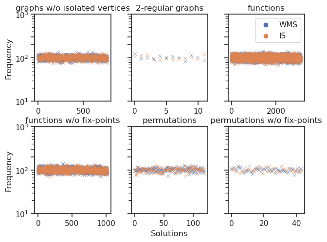
Figure 4: Uniformity comparison between an ideal sampler (IS) and our WMS.

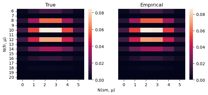
(a) friends-smokers

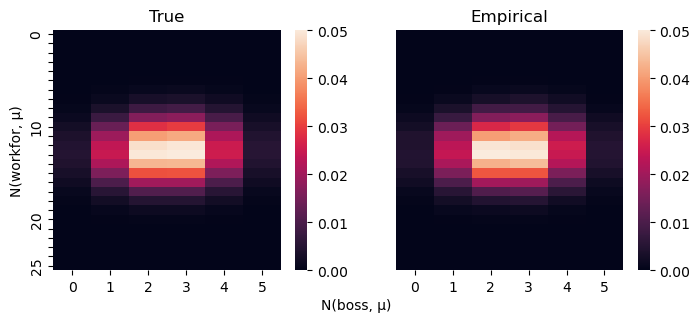
(b) employment

Figure 5: Conformity testing for the count distribution of MLNs.

For sampling problems from MLNs, enumerating all the models is infeasible even for a domain of size $5$, e.g., there are $2^{2^{5}+5}=2^{37}$ models in the employment MLN. That is why we test the count distribution of predicates from the problems. Instead of specifying the probability of each model, the count distribution only tells us the probability that a certain number of predicates are interpreted to be true in the models. An advantage of testing count distributions is that they can be efficiently computed for our MLNs. Please refer to [24] for more details about count distributions. We also note that the conformity of count distribution is a necessary condition for the correctness of algorithms. We kept the domain size to be $5$ and sampled $10^{5}$ models from friends-smokers and employment MLNs respectively. The empirical distributions of count-statistics, along with the true count distributions, are shown in Figure 5. It is easy to check the conformity of the empirical distribution to the true one from the figure. The statistical test was also performed on the count distribution, and the results confirm the conclusion drawn from the figure (also see E.2).

8.2 Performance

To evaluate the performance, we compared our weighted model samplers with Unigen [2, 32], the state-of-the-art approximate sampler for Boolean formulas. Note that there is no guarantee of polynomial complexity for Unigen, and its runtime highly depends on the underlying SAT solver it uses. We reduce the WFOMS problems to the sampling problems of Boolean formulas by grounding the input first-order sentence over the given domain. Since Unigen only works for uniform sampling, we employed the technique in [4] to encode the weighting function in the WFOMS problem into a Boolean formula.

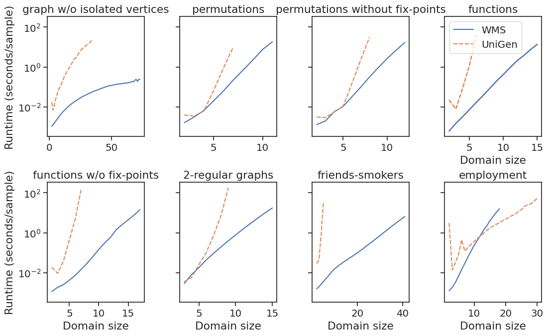
Figure 6: Performance of WMS versus UniGen.

For each sampling problem, we randomly generated $1000$ models by our WMS and Unigen respectively, and computed the average sampling time per one model. The performance comparison is shown in Figure 6. In most cases, our approach is much faster than UniGen. The exception in the employment MLN, where UniGen performed better than WMS, is likely due to the simplicity of this specific instance for its underlying SAT solver. This coincides with the theoretical result that our WMS is polynomial-time in the domain size, while UniGen usually needs amounts of expensive SAT calls on the grounded formulas.

9 Related Work

The studies on model counting and sampling problems date back to the 1970s [35, 36, 20]. In the seminal paper by Jerrum et al. [20], a significant connection was established between the random generation of combinatorial structures (i.e., model sampling) and the problem of model counting. Specifically, this paper showed that the random generation of combinatorial structures can be reduced in polynomial time to the model counting problem, under the condition of self-reducible. Self-reducibility refers to the property where the solution set for a given instance of a problem can be expressed in terms of the solution sets of smaller instances of the same problem. In the context of propositional logic, self-reducibility naturally holds as the solution set of a Boolean formula $\Gamma$ can be expressed in terms of the solution sets of $\Gamma_{a}$ and $\Gamma_{\neg a}$, where $a$ is an arbitrary atom in $\Gamma$, and $\Gamma_{a}$ and $\Gamma_{\neg a}$ are the formulas obtained from $\Gamma$ by setting $a$ to be true and false respectively. This property allows for a polynomial-time reduction from WMS to WMC, where the truth value of each atom in $\Gamma$ is incrementally sampled based on the ratio of the WMC of $\Gamma_{a}$ and $\Gamma_{\neg a}$. However, in first-order logic, self-reducibility is not generally guaranteed. Conditioning on a ground atom in a first-order sentence may make the resulting problem intractable, even if the original problem is tractable. For example, Van den Broeck and Davis [41] have proven that there exists a $\mathbf{UFO}^{2}$ sentence whose WFOMC with binary ground atoms cannot be computed in time polynomial in the size of the binary atoms, unless ¶=. This result implies that the reduction derived from self-reducibility is not applicable to WFOMS, motivating this paper to develop new techniques for sampling from first-order formulas.

The approach taken in this paper, as well as the formal liftability notions considered here, are inspired by the lifted inference literature [44]. In lifted inference, the goal is to perform probabilistic inference in statistical-relational models in a way that exploits symmetries in the high-level structure of the model. Models that are amenable to scalable inference as domain size increases are dubbed domain-liftable, in a similar spirit to the notion of domain-liftability under sampling presented here. There exists a very extensive literature on lifted inference, both viewed from the logical as well as graphical models perspective [27, 7, 13, 39, 33], which we do not cover exhaustively here for brevity. We do, however, draw the reader’s attention to Beame et al. [1, Appendix C], which studies the data complexity of WFOMC of $\mathbf{UFO}^{2}$. The general argument used there—namely, the analysis of a two-variable sentence in terms of its cell types—forms a basis for our sampling approaches discussed in the paper.

The domain recursion scheme, another important approach adopted in this paper, is similar to the domain recursion rule used in weighted first-order model counting [39, 21, 22, 34]. The domain recursion rule for WFOMC is a technique that utilizes a gradual grounding process on the input first-order sentence, where only one element of the domain is grounded at a time. As each element is grounded, the partially grounded sentence is simplified until the element is entirely removed, resulting in a new WFOMC problem with a smaller domain. With the domain recursion rule, one can apply the principle of induction on the domain size, and compute WFOMC by dynamic programming. A closely related work to this paper is the approach presented by Kazemi et al. [21], where they used the domain recursion rule to compute WFOMC of $\mathbf{FO}^{2}$ sentences without using Skolemization [43], which introduces negative weights. However, it is important to note that their approach can be only applied to some specific first-order formulas, whereas the domain recursion scheme presented in this paper, mainly designed for eliminating the existentially-quantified formulas, supports the entire $\mathbf{C}^{2}$ fragment with cardinality constraints.

It is also worth mentioning that weighted model sampling is a relatively well-studied area [14, 2, 3]. However, many real-world problems can be represented more naturally and concisely in first-order logic, and suffer from a significant increase in formula size when grounded out to propositional logic. For example, a formula of the form $\forall x\exists y:\varphi$ is encoded as a Boolean formula of the form $\bigwedge_{i=1}^{n}\bigvee_{j=1}^{n}l_{i,j}$, whose length is quadratic in the domain size $n$. Since even finding a solution to a such large ground formula is challenging, most sampling approaches for propositional logic instead focus on designing approximate samplers. We also note that these approaches are not polynomial-time in the length of the input formula, and rely on access to an efficient SAT solver. An alternative strand of research [17, 18, 11] on combinatorial sampling, focuses on the development of near-uniform and efficient sampling algorithms. However, these approaches can only be employed for specific Boolean formulas that satisfy a particular technical requirement known as the Lovász Local Lemma. The WFOMS problems studied in this paper do not typically meet the requisite criteria for the application of these techniques.

10 Conclusion and Future Work

In this paper, we prove the domain-liftability under sampling for the $\mathbf{C}^{2}$ fragment. The result is further extended to the fragment of $\mathbf{C}^{2}$ with the presence of cardinality constraints. The widespread applicability of WFOMS renders the proposed approach a promising candidate to serve as a universal paradigm for a plethora of sampling problems.

A potential avenue for further research is to expand the methodology presented in this paper to encompass more expressive first-order languages. Specifically, the utilization of the domain recursion scheme employed in this paper could be extended beyond the confines of $\mathbf{C}^{2}$, as its analogous technique, the domain recursion rule, has been demonstrated to be effective in proving the domain-liftability of the fragments $\mathbf{S}^{2}\mathbf{FO}^{2}{}$ and $\mathbf{S}^{2}\mathbf{RU}$ for WFOMC [22].

In addition to extending the input logic, other potential directions for future research include incorporating elementary axioms, such as tree axiom [37] and linear order axiom [34], as well as more general weighting functions that involve negative weights. However, it is important to note that these extensions would likely require a more advanced and nuanced approach than the one proposed in this paper, and may present significant challenges.

Finally, the lower complexity bound of WFOMS is also an interesting open problem. We have discussed in the introduction that it is unlikely for an (even approximate) lifted WMS to exist for full first-order logic. However, the establishment of a tighter lower bound for fragments of FO, such as $\mathbf{FO}^{3}$, remains an unexplored and challenging area that merits further investigation.

Appendix A WFOMC with Unary Evidence

In this section, we show how to deal with unary evidence in conditional WFOMC.

Van den Broeck and Davis [41] handled the unary evidence by the following transformation of the input sentence $\Gamma$. For any unary predicate $P$ appearing in the evidence, they split the domain into $\Delta_{\top}^{P}$, $\Delta_{\bot}^{P}$ and $\Delta_{\emptyset}^{P}$, where $\Delta_{\top}^{P}$ and $\Delta_{\bot}^{P}$ contains precisely the elements with evidence $P(a)$ and $\neg P(a)$, respectively, and $\Delta_{\emptyset}^{P}=\Delta\setminus(\Delta_{\top}^{P}\cup\Delta_{\bot}^{P})$ is the remaining elements. Then the sentence $\Gamma$ was transformed into

$$\left(\forall x\in\Delta_{\top}^{P}:\Gamma_{\top}^{P}\right)\land\left(\forall x\in\Delta_{\bot}^{P}:\Gamma_{\bot}^{P}\right)\land\left(\forall x\in\Delta_{\emptyset}^{P}:\Gamma\right),$$

where $\Gamma_{\top}^{P}$ and $\Gamma_{\bot}^{P}$ were obtained from $\Gamma$ by replacing all occurrences of $P$ with $\mathsf{True}$ and $\mathsf{False}$, respectively, and $\forall x\in\Delta^{\prime}$ was a domain constraint that restricts the quantifier to the domain $\Delta^{\prime}$. The procedure could be repeated to support multiple unary predicates, and the resulting sentence was then compiled into a FO d-DNNF circuits [42] for model counting. The domain constraints are natively supported by FO d-DNNF circuits, and the compilation and model counting has been shown to be in time polynomial in the domain size.

However, not all WFOMC algorithms can effectively support the domain constraints, and efficiently count the model of the transformed sentence. In the following, we provide a simpler approach to deal with the unary evidence, without the need for domain constraints.

We first introduce the notion of evidence type. An evidence type $\sigma$ over a predicate vocabulary $\mathcal{P}$ is a consistent set of 1-literals formed by $\mathcal{P}$. For instance, both $\{P(x),\neg Q(x)\}$ and $\{P(x)\}$ are evidence types over $\{P/1,Q/1\}$. The evidence type can be also viewed as a conjunction of its elements, where $\sigma(x)$ denotes a quantifier-free formula. If the evidence type $\sigma$ is an empty set, then $\sigma(x)$ is defined as $\top$. The number of evidence types over $\mathcal{P}$ is finite, and independent of the size of the domain. Given a set $L$ of ground 1-literals, the evidence type of an element is defined as the set of all literals in $L$ that are associated with the element. For example, if $L=\{P(a),\neg Q(a),R(b)\}$ and $\Delta=\{a,b,c\}$, then the evidence type of $a$ is $\{P(x),\neg Q(x)\}$, the evidence type of $b$ is $\{R(x)\}$, and the evidence type of $c$ is $\emptyset$.

See 1

Proof.

Let $\sigma^{1},\sigma^{2},\dots,\sigma^{m}$ be the distinct evidence types of elements given by $L$. The number of elements with evidence type $\sigma^{i}$ is denoted by $n_{i}$. We first transform the input sentence into

$$\Gamma^{\prime}:=\Gamma\land\bigwedge_{i\in[m]}(\forall x:\xi^{i}(x)\Rightarrow\sigma^{i}(x))\land\Lambda,$$

where each $\xi^{i}/1$ is a fresh predicate for $\sigma^{i}$ with the weight $w(\xi^{i})=\bar{w}(\xi^{i})=1$, and

$$\Lambda=\left(\forall x:\bigvee_{i\in[m]}\xi^{i}(x)\right)\land\left(\forall x:\bigwedge_{i,j\in[m]:i\neq j}(\neg\xi^{i}(x)\lor\neg\xi^{j}(x))\right).$$

The formula $\Lambda$ states that each element $a$ has exactly one True $\xi^{i}(a)$. In other words, the interpretation of predicates $\xi^{i}$ can be seen as a partition of the domain, where each disjoint subset in the partition contains precisely the elements with evidence type $\sigma^{i}$. Then we have

$$\mathsf{WFOMC}(\Gamma\land\bigwedge_{l\in L}l,\Delta,w,\bar{w})=\frac{1}{\binom{n}{n_{1},n_{2},\dots,n_{m}}}\cdot\mathsf{WFOMC}(\Gamma^{\prime}\land\bigwedge_{i\in[m]}(|\xi^{i}|=n_{i}),\Delta,w,\bar{w}),$$ (26)

where $|\xi^{i}|=n_{i}$ is a cardinality constraint that restricts the number of True $\xi^{i}$ in the model to be $n_{i}$. The reasoning is as follows. Denote by $k_{1},k_{2},\dots,k_{n}$ the indices of evidence type of each element in the domain, e.g., $\sigma^{k_{i}}$ is the evidence type of $i$-th element in the domain. It is easy to show that

$$\mathsf{WFOMC}(\Gamma\land\bigwedge_{l\in L}l,\Delta,w,\bar{w})=\mathsf{WFOMC}(\Gamma^{\prime}\land\bigwedge_{i\in[n]}\xi^{k_{i}}(e_{i}),\Delta,w,\bar{w}),$$ (27)

where $e_{i}$ is the $i$-th element in the domain. Next, let us consider the WFOMC problems of $\Gamma^{\prime}\land\bigwedge_{i\in[m]}(|\xi^{i}|=n_{i})$ and $\Gamma^{\prime}\land\bigwedge_{i\in[n]}\xi^{k_{i}}(e_{i})$. We view the interpretation of $\xi^{i}$ as an order dependent partition of the domain, and call $(|\xi^{1}|,|\xi^{2}|,\dots,|\xi^{m}|)$ the configuration of the partition. Then, the WFOMC of $\Gamma^{\prime}\land\bigwedge_{i\in[m]}(|\xi^{i}|=n_{i})$ can be written as the summation of the WFOMC of $\Gamma^{\prime}\land\bigwedge_{i\in[n]}\xi^{k_{i}^{\prime}}(e_{i})$ over all possible interpretations $\xi^{k_{i}^{\prime}}(e_{i})$, whose corresponding partition configuration is $(n_{1},\dots,n_{m})$. There are totally $\binom{n}{n_{1},n_{2},\dots,n_{m}}$ such interpretations, and the interpretation $\xi^{k_{i}}(e_{i})$ is one of them. Furthermore, due to the symmetry of WFOMC, all these interpretations have the same value of WFOMC. Thus, we can write

$$\mathsf{WFOMC}(\Gamma^{\prime}\land \bigwedge_{i\in[m]}(|\xi^{i}|=n_{i}),\Delta,w,\bar{w})$$ (28)

$$=\binom{n}{n_{1},n_{2},\dots,n_{m}}\cdot\mathsf{WFOMC}(\Gamma^{\prime}\land\bigwedge_{i\in[n]}\xi^{k_{i}}(e_{i}),\Delta,w,\bar{w}).$$

Combining (27) and (28) yields (26). Finally, computing the WFOMC in (26) has been shown to be in time polynomial in the domain size in [42] for any domain-liftable sentence $\Gamma$, which completes the proof. ∎

Appendix B Normal Forms

B.1 Scott Normal Form

We briefly describe the transformation of $\mathbf{FO}^{2}$ formulas to SNF and prove the soundness of its corresponding reduction on the WFOMS problems. The process is well-known, so we only sketch the related details.

Let $\Gamma$ be a sentence of $\mathbf{FO}^{2}$. To put it into SNF, consider a subformula $\varphi(x)=Qy:\phi(x,y)$, where $Q\in\{\forall,\exists\}$ and $\phi$ is quantifier-free. Let $A_{\varphi}$ be a fresh unary predicate and consider the sentence

$$\forall x:(A_{\varphi}(x)\Leftrightarrow(Qy:\phi(x,y)))$$

which states that $\varphi(x)$ is equivalent to $A_{\varphi}(x)$. Let $Q^{\prime}$ denote the dual of $Q$, i.e., $Q^{\prime}\in\{\forall,\exists\}\setminus\{Q\}$, this sentence can be seen equivalent to

$$\Gamma^{\prime}:= \forall xQy:(A_{\varphi}(x)\Rightarrow\phi(x,y))$$

$$\land\forall xQ^{\prime}y:(\phi(x,y)\Rightarrow A_{\varphi}(x)).$$

Let

$$\Gamma^{\prime\prime}:=\Gamma^{\prime}\land\Gamma[\varphi(x)/A_{\varphi}(x)],$$

where $\Gamma[\varphi(x)/A_{\varphi}(x)]$ is obtained from $\Gamma$ by replacing $\varphi(x)$ with $A_{\varphi}(x)$. For any domain $\Delta$, every model of $\Gamma^{\prime\prime}$ over $\Delta$ can be mapped to a unique model of $\Gamma$ over $\Delta$. The bijective mapping function is simply the projection $\langle\cdot\rangle_{\mathcal{P}_{\Gamma}}$. Let both the positive and negative weights of $A_{\varphi}$ be $1$ and denote the new weighting functions as $w^{\prime}$ and $\bar{w}^{\prime}$. It is clear that the reduction from $(\Gamma,\Delta,w,\bar{w})$ to $(\Gamma^{\prime\prime},\Delta,w^{\prime},\bar{w}^{\prime})$ is sound. Repeat this process from the atomic level and work upwards until the sentence is in SNF. The whole reduction remains sound due to the transitivity of soundness.

B.2 Normal Form for $\mathbf{C}^{2}$

We show that any $\mathbf{C}^{2}$ sentence can be converted into the normal form:

$$\Gamma_{\forall}\land\bigwedge_{i\in[m]}(\forall x:A_{i}(x)\Leftrightarrow(\exists_{=k_{i}}y:R_{i}(x,y))),$$

where $\Gamma_{\forall}$ is a $\mathbf{FO}^{2}$ sentence, each $k_{i}$ is a non-negative integer, $R_{i}(x,y)$ is an atomic formula, and $A_{i}$ is an unary predicate. The process is as follows:

1. Convert each counting-quantified formula of the form $\exists_{\geq k}y:\phi(x,y)$ to $\neg(\exists_{\leq k-1}y:\phi(x,y))$.

2. Decompose each $\exists_{\leq k}y:\phi(x,y)$ into $\bigvee_{i\in[0,k]}(\exists_{=i}y:\phi(x,y))$.

3. Replace each subformula $\exists_{=k}y:\phi(x,y)$, where $k>|\Delta|$, with False.

4. Starting from the atomic level and working upwards, replace any subformula $\exists_{=k}\phi(x,y)$, where $\phi(x,y)$ is a formula that does not contain any counting quantifier, with $A(x)$; and append $\forall x\forall y:R(x,y)\Leftrightarrow\phi(x,y)$ and $\forall x:A(x)\Leftrightarrow(\exists_{=k}y:R(x,y))$, where $R$ is an auxiliary binary predicate, to the original sentence.

It is easy to check that the reduction presented above is sound and independent of the domain size if the domain size is greater than the maximum counting parameter $k$ in the input sentence.

Appendix C A Sound Reduction from $\mathbf{SC}^{2}$ to $\mathbf{FO}^{2}$ with Cardinality Constraints

In this section, we show the sound reduction from a WFOMS problem on $\mathbf{SC}^{2}$ sentence to a WFOMS problem on $\mathbf{FO}^{2}$ sentence with cardinality constraints.

We first need the following two lemmas, which are based on the transformations from [24].

Lemma 8.

Let $\Gamma$ be a first-order logic sentence, and let $\Delta$ be a domain. Let $\Phi$ be a first-order sentence with cardinality constraints, defined as follows:

$$\Pi:= (|P|=k\cdot|\Delta|)$$

$$\land(\forall x\forall y:P(x,y)\Leftrightarrow(R_{1}^{P}(x,y)\lor\dots\lor R_{k}^{P}(x,y)))$$

$$\land\bigwedge_{i\in[k]}(\forall x\exists y:R_{i}^{P}(x,y))$$

$$\land\bigwedge_{i,j\in[k]:i\neq j}(\forall x\forall y:\neg R_{i}^{P}(x,y)\lor\neg R_{j}^{P}(x,y)),$$

where $R_{i}^{P}$ are auxiliary predicates not in $\mathcal{P}_{\Gamma}$ with weight $w(R_{i}^{P})=\bar{w}(R_{i}^{P})=1$. Then the reduction from the WFOMS $(\Gamma\land\forall x\exists_{=k}y:P(x,y),\Delta,w,\bar{w})$ to $(\Gamma\land\Pi,\Delta,w,\bar{w})$ is sound.

Proof.

Let $f(\cdot)=\langle\cdot\rangle_{\mathcal{P}_{\Gamma}\cup\{P\}}$ be a mapping function. We first show that $f$ is from $\mathcal{M}_{\Gamma\land\Pi,\Delta}$ to $\mathcal{M}_{\Gamma\land\forall x\exists_{=k}:P(x,y),\Delta}$: if $\mathcal{A}\models\Gamma\land\Pi$ then $f(\mathcal{A})\models\Gamma\land\forall x\exists_{=k}y:P(x,y)$.

The sentence $\Pi$ means that for every $c_{1},c_{2}\in\Delta$ such that $P(c_{1},c_{2})$ is true, there is exactly one $i\in[k]$ such that $R_{i}^{P}(c_{1},c_{2})$ is true. Thus we have that $\sum_{i\in[k]}|R_{i}^{P}|=|P|=k\cdot|\Delta|$, which together with $\bigwedge_{i\in[k]}\forall x\exists y:R_{i}^{P}(x,y)$ implies that $|R_{i}^{P}|=k$ for $i\in[k]$. We argue that each $R_{i}^{P}$ is a function predicate in the sense that $\forall x\exists_{=1}y:R_{i}^{P}(x,y)$ holds in any model of $\Gamma\land\Pi$. Let us suppose, for contradiction, that $(\forall x\exists y:R_{i}^{P}(x,y))\land(|R_{i}^{P}|=k)$ holds but there is some $a\in\Delta$ such that $R_{i}^{P}(a,b)$ and $R_{i}^{P}(a,b^{\prime})$ are true for some $b\neq b^{\prime}\in\Delta$. We have $|\{(x,y)\in\Delta^{2}\mid R_{i}^{P}(x,y)\land x\neq a\}|\geq|\Delta|-1$ by the fact $\forall x\exists y:R_{i}^{P}(x,y)$. It follows that $|R_{i}^{P}|\geq|\{(x,y)\in\Delta^{2}\mid R_{i}^{P}(x,y)\land x\neq a\}|+2>|\Delta|$, which leads to a contradiction. Since all of $R_{i}^{P}$ are function predicates, it is easy to check $\forall x\exists_{=k}y:P(x,y)$ must be true in any model $\mu$ of $\Gamma\land\Pi$, i.e., $f(\mu)\models\Gamma\land\forall x\exists_{=k}y:P(x,y)$.

To finish the proof, one can easily show that, for every model $\mu\in\mathcal{M}_{\Gamma\land\forall x\exists_{=k}y:P(x,y),\Delta}$, there are exactly $(k!)^{|\Delta|}$ models $\mu^{\prime}\in\mathcal{M}_{\Gamma\land\Pi,\Delta}$ such that $f(\mu^{\prime})=\mu$. The reason for this is that 1) if, for any $a\in\Delta$, we permute $b_{1},b_{2},\dots,b_{k}$ in $R_{1}^{P}(a,b_{1}),R_{2}^{P}(a,b_{2}),\dots,R_{k}^{P}(a,b_{k})$ in the model $\mu^{\prime}$, we get another model of $\Gamma\land\Pi$, and 2) up to these permutations, the predicates $R_{i}^{P}$ in $\mu^{\prime}$ are determined uniquely by $\mu$. Finally, the weights of all these $\mu^{\prime}$ are the same as those of $\mu$, and we can write

$$\sum_{\begin{subarray}{c}\mu^{\prime}\in\mathcal{M}_{\Gamma\land\Pi,\Delta}:\\ f(\mu^{\prime})=\mu\end{subarray}}\mathbb{P}[\mu^{\prime}\mid\Gamma\land\Pi] =\frac{\sum_{\begin{subarray}{c}\mu^{\prime}\in\mathcal{M}_{\Gamma\land\Pi,\Delta}:\\ f(\mu^{\prime})=\mu\end{subarray}}\langle w,\bar{w}\rangle(\mu^{\prime})}{\mathsf{WFOMC}(\Gamma\land\Pi,\Delta,w,\bar{w})}$$

$$=\frac{(k!)^{|\Delta|}\cdot\langle w,\bar{w}\rangle(\mu)}{(k!)^{|\Delta|}\cdot\mathsf{WFOMC}(\Gamma\land\forall x\exists_{=k}y:P(x,y),\Delta,w,\bar{w})}$$

$$=\frac{\langle w,\bar{w}\rangle(\mu)}{\mathsf{WFOMC}(\Gamma\land\forall x\exists_{=k}y:P(x,y),\Delta,w,\bar{w})}$$

$$=\mathbb{P}[\mu\mid\Gamma\land\forall x\exists_{=k}y:P(x,y)],$$

which completes the proof. ∎

Lemma 9.

Let $\Gamma$ be a first-order logic sentence, $\Delta$ be a domain, and $P$ be a predicate. Then the WFOMS $(\Gamma\land\forall_{=k}\forall y:P(x,y),\Delta,w,\bar{w})$ can be reduced to $(\Gamma\land(|U|=k)\land(\forall x:U(x)\Leftrightarrow(\forall y:P(x,y))),\Delta,w,\bar{w})$, where $U$ is an auxiliary unary predicate with weight $w(U)=\bar{w}(U)=1$, and the reduction is sound.

Proof.

The proof is straightforward. ∎

Proof of Lemma 7.

We can first get rid of all formulas of the form $\exists_{=k}x\forall y:P(x,y)$ by repeatedly using Lemma 9. Then we can use Lemma 8 repeatedly to eliminate the formulas of the form $\forall x\exists_{=k}y:P(x,y)$. The whole reduction is sound due to the transitivity of soundness. ∎

Appendix D Missing Details of WMS

D.1 Optimizations for WMS

There exist several optimizations to make the sampling algorithm more practical. Here, we present some of them that are used in our implementation.

Heuristic method for element selection

The complexity of TwoTablesSampler heavily depends on the recursion depth. In our implementation, when selecting a domain element $e_{t}$ for sampling its substructure, we always chose the element with the “strongest” existential constraint that contains the most Tseitin atoms $Z_{k}(x)$. It would help TwoTablesSampler reach the condition that the existential constraint for all elements is $\top$. In this case, TwoTablesSampler will invoke the more efficient WMS for $\mathbf{UFO}^{2}$ to sample the remaining substructures.

Further decomposition of 2-tables sampling

Let $\mathcal{P}_{\exists}$ be the union of predicates vocabularies of the existentially quantified formulas

$$\mathcal{P}_{\exists}:=\{R_{1},R_{2},\dots,R_{m}\}.$$

We further decomposed the sampling probability of 2-tables $\mathbb{P}[\mathcal{A}\mid\Gamma_{T}\land\bigwedge_{i\in[n]}\eta_{i}(e_{i})]$ into

$$\mathbb{P}\left[\mathcal{A}\mid\Gamma_{T}\land\bigwedge_{i\in[n]}\eta_{i}(e_{i})\land\mathcal{A}_{\exists}\right]\cdot\mathbb{P}\left[\mathcal{A}_{\exists}\mid\Gamma_{T}\land\bigwedge_{i\in[n]}\eta_{i}(e_{i})\right],$$

where $\mathcal{A}_{\exists}$ is a $\mathcal{P}_{\exists}$-structure over $\Delta$. It decomposes the conditional sampling problem of $\mathcal{A}$ into two subproblems—one is to sample $\mathcal{A}_{\exists}$ and the other to sample the remaining substructures conditional on $\mathcal{A}_{\exists}$. The subproblem of sampling $\mathcal{A}$ conditioned on $\mathcal{A}_{\exists}$ can be reduced into a sampling problem on a $\mathbf{UFO}^{2}$ sentence with evidence

$$\Gamma^{\prime}=\forall x\forall y:\psi(x,y)\land\bigwedge_{i\in[m]}\tau_{i}(e_{i})\land\mathcal{A}_{\exists},$$ (29)

since all existentially-quantified formulas have been satisfied with $\mathcal{A}_{\exists}$. Recall that for a $\mathbf{UFO}^{2}$ sentence, when the 1-types $\tau_{i}$ of all elements has been fixed, the sampling problem of 2-tables can be decomposed into multiple independent sampling problems of the 2-table for each elements tuple (see Section 4.2). Sampling 2-tables from (29) can be solved in a similar way, by decomposing the sampling probability into

$$\mathbb{P}\left[\bigwedge_{i,j\in[n]:i<j}\pi_{i,j}(e_{i},e_{j})\mid\Gamma^{\prime}\right]=\prod_{i,j\in[n]:i<j}\mathbb{P}\left[\pi_{i,j}(e_{i},e_{j})\mid\psi^{\prime}(e_{i},e_{j})\right],$$

where $\psi^{\prime}(e_{i},e_{j})$ is the simplified formula of $\psi(e_{i},e_{j})\land\psi(e_{j},e_{i})$ obtained by replacing the ground 1-literals with their truth values by the 1-types $\tau_{i}(e_{i})$ and $\tau_{j}(e_{j})$, and the sampled structure $\mathcal{A}_{\exists}$. The 2-tables $\pi_{i,j}$ as well as the simplified formulas $\psi^{\prime}(e_{i},e_{j})$ are independent of each other, and thus can be efficiently sampled in parallel. The other subproblem of sampling $\mathcal{A}_{\exists}$ can be solved by an algorithm similar to TwoTablesSampler. In this algorithm, the 2-tables used to partition cells are now defined over $\mathcal{P}_{\exists}$, whose size is only $4^{m}$. Compared to the number $4^{B}$ of 2-tables in the original algorithm TwoTablesSampler, where $B\geq m$ is the number of binary predicates in $\Gamma$, the number of 2-tables in the new algorithm can be exponentially smaller. As a result, the for-loop that enumerates all 2-tables configurations in Algorithm 1 will be exponentially faster.

Cache

We cached the weight $\langle w,\bar{w}\rangle(\tau^{i})$ of all 1-types and the weight $\langle w,\bar{w}\rangle(\pi^{i})$ of all 2-tables, which are often used in our WMS.

D.2 The Submodule $\textsf{ExSat}(\cdot,\cdot)$

The pseudo-code of ExSat is presented in Algorithm 3.

Algorithm 3 ExSat($\mathbf{g},\eta$)

1:Decompose $\mathbf{g}$ into $\{g_{\eta^{i},\pi^{j}}\}_{i\in[N_{c}],j\in[N_{b}]}$

2:$(\beta,\tau)\leftarrow(\eta)$

3:// Check the coherence of 2-tables

4:for $i\in[N_{u}]$ do

5:     for $j\in[N_{b}]$ do

6:         // $\tau(\eta^{i})$ is the 1-type in $\eta^{i}$

7:         if $\pi^{j}$ is not coherent with $\tau(\eta^{i})$ and $\tau$ and $g_{\eta^{i},\pi^{j}}>0$ then

8:              return False

9:         end if

10:     end for

11:end for

12:// Check the satisfaction of existentially-quantified formulas

13:$\forall j\in[N_{b}],h_{\pi^{j}}\leftarrow\sum_{i\in[N_{c}]}g_{\eta^{i},\pi^{j}}$

14:for $Z_{k}(x)\in\beta$ do

15:     for $j\in[N_{b}]$ do

16:         if $R_{k}(x,y)\in\pi^{j}$ and $h_{\pi^{j}}>0$ then

17:              return True

18:         end if

19:     end for

20:end for

21:return False

Appendix E Missing Details of Experiments

E.1 Experiment Settings

Sampling Combinatorial Structures

The corresponding WFOMS problems for the uniform generation of combinatorial structures used in our experiments are presented as follows. The weighting functions $w$ and $\bar{w}$ map all predicates to $1$.

• Functions:

  $$\forall x\exists_{=1}y:f(x,y).$$

• Functions w/o fix points:

  $$(\forall x\exists_{=1}y:f(x,y))\land(\forall x:\neg f(x,x)).$$

• Permutations:

  $$(\forall x\exists_{=1}y:Per(x,y))\land(\forall y\exists_{=1}x:Per(x,y)).$$

• Permutation without fix-points:

  $$(\forall x\exists_{=1}y:Per(x,y))\land(\forall y\exists_{=1}x:Per(x,y))\land(\forall x:\neg Per(x,x)).$$

Sampling from MLNs

An MLN is a finite set of weighted first-order formulas $\{(w_{i},\alpha_{i})\}_{i\in[m]}$, where each $w_{i}$ is either a real-valued weight or $\infty$, and $\alpha_{i}$ is a first-order formula. Let $\mathcal{P}$ be the vocabulary of $\alpha_{1},\alpha_{2},\dots,\alpha_{m}$. An MLN $\Phi$ paired with a domain $\Delta$ induces a probability distribution over $\mathcal{P}$-structures (also called possible worlds):

$$p_{\Phi,\Delta}(\omega):=\begin{cases}\frac{1}{Z_{\Phi,\Delta}}\exp\left(\sum_{(\alpha,w)\in\Phi w\cdot\#(\alpha,\omega)\right)&\textrm{if }\omega\models\Phi_{\infty}\\ 0&\textrm{otherwise}\end{cases}}$$

where $\Phi$ and $\Phi_{\infty}$ are the real-valued and $\infty$-valued formulas in $\Phi$ respectively, and $\#(\alpha,\omega)$ is the number of groundings of $\alpha$ satisfied in $\omega$. The sampling problem on an MLN $\Phi$ over a domain $\Delta$ is to randomly generate a possible world $\omega$ according to the probability $p_{\Phi,\Delta}(\omega)$.

The reduction from the sampling problems on MLNs to WFOMS can be performed following the same idea as in [42]. For every real-valued formula $(\alpha_{i},w_{i})\in\Phi$, where the free variables in $\alpha_{i}$ are $\mathbf{x}$, we introduce a novel auxiliary predicate $\xi_{i}$ and create a new formula $\forall\mathbf{x}:\xi_{i}(\mathbf{x})\Leftrightarrow\alpha_{i}(\mathbf{x})$. For formula $\alpha_{i}$ with infinity weight, we instead create a new formula $\forall\mathbf{x}:\alpha_{i}(\mathbf{x})$. Denote the conjunction of the resulting set of sentences by $\Gamma$, and set the weighting function to be $w(\xi_{i})=\exp(w_{i})$ and $\bar{w}(\xi_{i})=1$, and for all other predicates, we set both $w$ and $\bar{w}$ to be $1$. Then the sampling problem on $\Phi$ over $\Delta$ is reduced to the WFOMS $(\Gamma,\Delta,w,\bar{w})$.

By the reduction above, we can write the two MLNs used in our experiments to WFOMS problems. The weights of predicates are all set to be $1$ unless otherwise specified.

• Friends-smokers MLN: the reduced sentence is

  $$\forall x:\neg fr(x,x)\land sm(x)\land$$

  $$\forall x\forall y:fr(x,y)\Leftrightarrow fr(y,x)\land$$

  $$\forall x\forall y:\xi(x,y)\Leftrightarrow(fr(x,y)\land sm(x)\Rightarrow sm(y))\land$$

  $$\forall x\exists y:fr(x,y),$$

  and the weight of $\xi$ is set to be $w(\xi)=\exp(0.2)$.

• Employment MLN: the corresponding sentence is

  $$\forall x:\xi(x)\Leftrightarrow(\exists y:workfor(x,y)\lor boss(x)),$$

  and the weight of $\xi$ is set to be $\exp(1.3)$.

E.2 More Experimental Results

We utilized the Kolmogorov-Smirnov (KS) test [25] to validate the conformity of the (count) distributions produced by our algorithm to the reference distributions. The KS test used here is based on the multivariate Dvoretzky–Kiefer–Wolfowitz (DKW) inequality recently proved by [26].

Let $\mathbf{X}_{1}=(X_{1i})_{i\in[k]},\mathbf{X}_{2}=(X_{2i})_{i\in[k]},\dots,\mathbf{X}_{n}=(X_{ni})_{i\in[k]}$ be $n$ real-valued independent and identical distributed multivariate random variables with cumulative distribution function (CDF) $F(\cdot)$. Let $F_{n}(\cdot)$ be the associated empirical distribution function defined by

$$F_{n}(\mathbf{x}):=\frac{1}{n}\sum_{i\in[n]}\mathbbm{1}_{X_{i1}\leq x_{1},X_{i2}\leq x_{2},\dots,X_{ik}\leq x_{k}},\qquad\mathbf{x}\in^{k}.$$

The DKW inequality states

$$\mathbb{P}\left[\sup_{\mathbf{x}\in^{k}}|F_{n}(\mathbf{x})-F(\mathbf{x})|>\epsilon\right]\geq(n+1)ke^{-2n\epsilon^{2}}$$ (30)

for every $\epsilon,n,k>0$. When the random variables are univariate, i.e., $k=1$, we can replace $(n+1)k$ in the above probability bound by a tighter constant $2$.

Table 2: The Kolmogorov-Smirnov Test

Problem	Maximum deviation	Upper bound
graphs w/o isolated vertices	0.0036	0.0049
2-regular graphs	0.0065	0.0069
functions	0.0013	0.0024
functions w/o fix-points	0.0027	0.0042
permutations	0.0071	0.0124
permutations w/o fix-points	0.019	0.02
friends-smokers	0.0021	0.0087
employment	0.0030	0.0087

In the KS test, the null hypothesize is that the samples $\mathbf{X}_{1},\mathbf{X}_{2},\dots,\mathbf{X}_{n}$ are distributed according to some reference distribution, whose CDF is $F(\cdot)$. By (30), with probability $1-\alpha$, the maximum deviation $\sup_{\mathbf{x}\in^{k}}|F_{n}(\mathbf{x})-F(\mathbf{x})|$ between empirical and reference distributions is bounded by $\epsilon=\sqrt{\frac{\ln(k(n+1)/\alpha)}{2n}}$ ($\frac{\sqrt{\ln(2/\alpha)}}{2n}$ for the univariate case). If the actual value of the maximum deviation is larger than $\epsilon$, we can reject the null hypothesis at the confidence level $\alpha$. Otherwise, we cannot reject the null hypothesis, i.e., the empirical distribution of the samples is not statistically different from the reference one. In our experiments, we choose $\alpha=0.05$ as a significant level.

For the uniform generation of combinatorial structures, we assigned each model a lexicographical number and treated the model indices as a multivariate random variable with a discrete multi-dimensional uniform distribution. For the sampling problems of MLNs, we test their count distributions against the true count distributions. Table 2 shows the maximum deviation between the empirical and reference cumulative distribution functions, along with the upper bound set by the DKW inequality. As shown in Table 2, all maximum deviations are within their respective upper bounds. Therefore, we cannot reject any null hypotheses, i.e., there is no statistically significant difference between the two sets of distributions.

Appendix F Missing Proofs

See 5

Proof.

Following a similar argument as in the proof of Lemma 2, the soundness of the reduction can be proved by showing that the function $f(\mu^{\prime})=\mu^{\prime}\cup\mathcal{A}_{t}\cup\tau_{t}(e_{t})$ is bijective. Let $\Lambda$ be the conjunction of

$$\forall x:\left(Z^{\exists}_{j,q}(x)\Leftrightarrow(\exists_{=q}y:R_{j}(x,y))\right)\land\left(Z^{\nexists}_{j,q}(x)\Leftrightarrow\neg(\exists_{=q}y:R_{j}(x,y))\right)$$

over all $j\in[m]$ and $q\in[0,k_{j}]$. We write the sentence ${\widetilde{\Gamma}}$ and ${\widetilde{\Gamma}}^{\prime}$ as

$${\widetilde{\Gamma}} =\Gamma_{\forall}\land\bigwedge_{i\in[n]}\left(\tau_{i}(e_{i})\land\nu_{i}(e_{i})\right)\land\mathcal{A}_{t}\land\Lambda$$

$${\widetilde{\Gamma}}^{\prime} =\Gamma_{\forall}\land\bigwedge_{i\in[n]\setminus\{t\}}\left(\tau_{i}(e_{i})\land({\nu_{i}}\downarrow{{\pi_{t,i}}})(e_{i})\right)\land\Lambda.$$

($\Rightarrow$)

For any model $\mu^{\prime}$ in $\mathcal{M}_{{\widetilde{\Gamma}}^{\prime},\Delta^{\prime}}$, we will prove that $f(\mu^{\prime})=\mu^{\prime}\cup\mathcal{A}_{t}\cup\tau_{t}(e_{t})$ is a model in $\mathcal{M}_{{\widetilde{\Gamma}},\Delta}$. First, one can easily check that $f(\mu^{\prime})$ satisfies $\Gamma_{\forall}\land\bigwedge_{i\in[n]}\tau_{i}(e_{i})$ by the satisfiability of ${\widetilde{\Gamma}}$. Next, we will demonstrate that $f(\mu^{\prime})$ also satisfies $\bigwedge_{i\in[n]}\nu(e_{i})\land\Lambda$. For any index $i\in[n]\setminus\{t\}$, any $j\in[n],q\in[0,k_{j}]$ such that $Z_{j,q}^{\exists}(x)\in\nu_{i}$, it can be easily shown that there exist exact $q$ ground atoms $R_{j}(e_{i},e)$ in $f(\mu^{\prime})$ by the definition of ${\nu_{i}}\downarrow{{\pi_{t,i}}}$. Thus, the counting quantified formula $\exists_{=q}y:R_{j}(e_{i},y)$ is true in $f(\mu^{\prime})$. Then let us consider the case of $\neg(\exists_{q}y:R_{j}(e_{i},y))$. For any $j\in[n],q\in[0,k_{j}]$ such that $Z_{j,q}^{\nexists}(x)\in\nu_{i}$, if $q>0$ or $R_{j}(e_{i},e_{t})\notin\mathcal{A}_{t}$, there must not exist $q$ ground atoms $R_{j}(e_{i},e)$ in $f(\mu^{\prime})$ following the similar argument as above. If $q=0$ and $R_{j}(e_{i},e_{t})\in\mathcal{A}_{t}$, the counting quantified formula $\neg(\exists_{=0}R_{j}(e_{i},y))$ is true in $\mathcal{A}_{t}$, and thus also satisfied in $f(\mu^{\prime})$. Finally, by the satisfability of ${\widetilde{\Gamma}}$, we have that $\nu_{t}(e_{t})\land\Lambda$ is true in $\mathcal{A}_{t}$. Therefore, we can conclude that $f(\mu^{\prime})$ satisfies $\bigwedge_{i\in[n]}\nu(e_{i})\land\Lambda$, which together with the satisfaction of $\Gamma_{\forall}\land\bigwedge_{i\in[n]}\tau_{i}(e_{i})$, implies that $f(\mu^{\prime})$ is a model in $\mathcal{M}_{{\widetilde{\Gamma}},\Delta}$.

($\Leftarrow$)

For any model $\mu$ in $\mathcal{M}_{{\widetilde{\Gamma}},\Delta}$, we will prove that $\mu^{\prime}=\mu\setminus(\mathcal{A}_{t}\cup\tau_{t}(e_{t}))$ is the unique model in $\mathcal{M}_{{\widetilde{\Gamma}}^{\prime},\Delta^{\prime}}$ such that $f(\mu^{\prime})=\mu$. The uniqueness of $\mu^{\prime}$ is clear from the definition of $f$. Since $\mu$ is a model of ${\widetilde{\Gamma}}$, we first have that $\mu^{\prime}$ satisfies $\Gamma_{\forall}\land\bigwedge_{i\in[n]\setminus\{t\}}\tau_{i}(e_{i})$. Then we will show that $\mu^{\prime}$ also satisfies $\bigwedge_{i\in[n]\setminus\{t\}}({\nu_{i}}\downarrow{{\pi_{t,i}}})(e_{i})\land\Lambda$. For any $i\in[n]$, by the definition of the block type, it is easy to check that there are exact $q$ ground atoms $R_{j}(e_{i},e)$ in $\mu$ for all $j\in[m],q\in[0,k_{j}]$ such that $Z^{\exists}_{j,q}(x)\in\nu_{i}$. Therefore, if $R_{j}(y,x)\in\pi_{t,i}$, we have that there exist exact $q-1$ ground atoms $R_{j}(e_{i},e)$ in $\mu^{\prime}$. Otherwise, the number of ground atoms $R_{j}(e_{i},e)$ in $\mu^{\prime}$ remains $q$. It follows that $\exists_{=s}y:R_{j}(e_{i},y)$ is true in $\mu^{\prime}$ for all $j\in[m],s\in[0,k_{j}]$ such that $Z_{j,s}^{\exists}(x)\in{\nu_{i}}\downarrow{{\pi_{t,i}}}$. The argument for the case of $\neg(\exists_{=s}y:R_{j}(e_{i},y))$ is similar. Hence, we have that $\mu^{\prime}$ satisfies $\bigwedge_{i\in[n]\setminus\{t\}}({\nu_{i}}\downarrow{{\pi_{t,i}}})(e_{i})\land\Lambda$, which combined with the satisfaction of $\forall x\forall y:\psi(x,y)\land\bigwedge_{i\in[n]\setminus\{t\}}\tau_{i}(e_{i})$ leads to conclusion.

By the bijectivity of the mapping function $f$, it is easy to prove the consistency of sampling probability through the reduction. The argument is the same as in the proof of Lemma 2. ∎

See 6

Proof.

The proof follows the same argument for Lemma 5. The only statement that needs to be argued is the bijectivity of the mapping function $f(\mu^{\prime})=\mu^{\prime}\cup\mathcal{A}_{t}\cup\tau_{t}(e_{t})$. For any model $\mu^{\prime}$ in $\mathcal{M}_{{\widetilde{\Gamma}}^{\prime},\Delta^{\prime}}$, $\mu^{\prime}$ satisfies both ${\widetilde{\Gamma}}^{\prime}$ and $\Upsilon^{\prime}$. It follows that $f(\mu^{\prime})$ satisfies both ${\widetilde{\Gamma}}$ and $\Upsilon$. For any model $\mu$ in $\mathcal{M}_{{\widetilde{\Gamma}},\Delta}$, the reasoning is similar, and we have that $f^{-1}(\mu)=\mu\setminus(\mathcal{A}_{t}\cup\tau_{t}(e_{t}))$ is a unique model in $\mathcal{M}_{{\widetilde{\Gamma}}^{\prime},\Delta^{\prime}}$. This establishes the bijectivity of $f$. The remainder of the proof, including the consistency of sampling probability, proceeds exactly the same as Lemma 2. ∎

References

- Beame et al. [2015] Paul Beame, Guy Van den Broeck, Eric Gribkoff, and Dan Suciu. Symmetric weighted first-order model counting. In Proceedings of the 34th ACM SIGMOD-SIGACT-SIGAI Symposium on Principles of Database Systems, pages 313–328, 2015.
- Chakraborty et al. [2013] Supratik Chakraborty, Kuldeep S Meel, and Moshe Y Vardi. A scalable and nearly uniform generator of sat witnesses. In International Conference on Computer Aided Verification, pages 608–623. Springer, 2013.
- Chakraborty et al. [2015a] Supratik Chakraborty, Daniel J Fremont, Kuldeep S Meel, Sanjit A Seshia, and Moshe Y Vardi. On parallel scalable uniform sat witness generation. In International Conference on Tools and Algorithms for the Construction and Analysis of Systems, pages 304–319. Springer, 2015a.
- Chakraborty et al. [2015b] Supratik Chakraborty, Dror Fried, Kuldeep S Meel, and Moshe Y Vardi. From weighted to unweighted model counting. In Twenty-Fourth International Joint Conference on Artificial Intelligence, 2015b.
- Chavira and Darwiche [2008] Mark Chavira and Adnan Darwiche. On probabilistic inference by weighted model counting. Artificial Intelligence, 172(6-7):772–799, 2008.
- Cooper et al. [2007] Colin Cooper, Martin Dyer, and Catherine Greenhill. Sampling regular graphs and a peer-to-peer network. Combinatorics, Probability and Computing, 16(4):557–593, 2007.
- de Salvo Braz et al. [2005] Rodrigo de Salvo Braz, Eyal Amir, and Dan Roth. Lifted first-order probabilistic inference. In IJCAI, pages 1319–1325. Professional Book Center, 2005.
- Domshlak and Hoffmann [2007] Carmel Domshlak and Jörg Hoffmann. Probabilistic planning via heuristic forward search and weighted model counting. Journal of Artificial Intelligence Research, 30:565–620, 2007.
- Dyer et al. [2002] Martin Dyer, Alan Frieze, and Mark Jerrum. On counting independent sets in sparse graphs. SIAM Journal on Computing, 31(5):1527–1541, 2002.
- Erdős et al. [1960] Paul Erdős, Alfréd Rényi, et al. On the evolution of random graphs. Publ. Math. Inst. Hung. Acad. Sci, 5(1):17–60, 1960.
- Feng et al. [2021] Weiming Feng, Kun He, and Yitong Yin. Sampling constraint satisfaction solutions in the local lemma regime. In Proceedings of the 53rd Annual ACM SIGACT Symposium on Theory of Computing, pages 1565–1578, 2021.
- Gao and Wormald [2015] Pu Gao and Nicholas Wormald. Uniform generation of random regular graphs. In 2015 IEEE 56th Annual Symposium on Foundations of Computer Science, pages 1218–1230. IEEE, 2015.
- Gogate and Domingos [2011] Vibhav Gogate and Pedro M. Domingos. Probabilistic theorem proving. In UAI, pages 256–265. AUAI Press, 2011.
- Gomes et al. [2021] Carla P Gomes, Ashish Sabharwal, and Bart Selman. Model counting. In Handbook of satisfiability, pages 993–1014. IOS press, 2021.
- Grädel et al. [1997] Erich Grädel, Phokion G Kolaitis, and Moshe Y Vardi. On the decision problem for two-variable first-order logic. Bulletin of symbolic logic, 3(1):53–69, 1997.
- Gradel et al. [1997] Erich Gradel, Martin Otto, and Eric Rosen. Two-variable logic with counting is decidable. In Proceedings of Twelfth Annual IEEE Symposium on Logic in Computer Science, pages 306–317. IEEE, 1997.
- Guo et al. [2019] Heng Guo, Mark Jerrum, and Jingcheng Liu. Uniform sampling through the lovász local lemma. Journal of the ACM (JACM), 66(3):1–31, 2019.
- He et al. [2021] Kun He, Xiaoming Sun, and Kewen Wu. Perfect sampling for (atomic) lov'asz local lemma. arXiv preprint arXiv:2107.03932, 2021.
- Jaeger [2015] Manfred Jaeger. Lower complexity bounds for lifted inference. Theory and Practice of Logic Programming, 15(2):246–263, 2015.
- Jerrum et al. [1986] Mark Jerrum, Leslie G. Valiant, and Vijay V. Vazirani. Random generation of combinatorial structures from a uniform distribution. Theor. Comput. Sci., 43:169–188, 1986.
- Kazemi et al. [2016] Seyed Mehran Kazemi, Angelika Kimmig, Guy Van den Broeck, and David Poole. New liftable classes for first-order probabilistic inference. Advances in Neural Information Processing Systems, 29, 2016.
- Kazemi et al. [2017] Seyed Mehran Kazemi, Angelika Kimmig, Guy Van den Broeck, and David Poole. Domain recursion for lifted inference with existential quantifiers. arXiv preprint arXiv:1707.07763, 2017.
- Kuusisto and Lutz [2018] Antti Kuusisto and Carsten Lutz. Weighted model counting beyond two-variable logic. In Proceedings of the 33rd Annual ACM/IEEE Symposium on Logic in Computer Science, pages 619–628, 2018.
- Kuzelka [2021] Ondrej Kuzelka. Weighted first-order model counting in the two-variable fragment with counting quantifiers. Journal of Artificial Intelligence Research, 70:1281–1307, 2021.
- Massey Jr [1951] Frank J Massey Jr. The kolmogorov-smirnov test for goodness of fit. Journal of the American statistical Association, 46(253):68–78, 1951.
- Naaman [2021] Michael Naaman. On the tight constant in the multivariate dvoretzky–kiefer–wolfowitz inequality. Statistics & Probability Letters, 173:109088, 2021.
- Poole [2003] David Poole. First-order probabilistic inference. In IJCAI, pages 985–991. Morgan Kaufmann, 2003.
- Raedt et al. [2007] Luc De Raedt, Angelika Kimmig, and Hannu Toivonen. Problog: A probabilistic prolog and its application in link discovery. In Manuela M. Veloso, editor, IJCAI 2007, Proceedings of the 20th International Joint Conference on Artificial Intelligence, Hyderabad, India, January 6-12, 2007, pages 2462–2467, 2007.
- Richardson and Domingos [2006] Matthew Richardson and Pedro Domingos. Markov logic networks. Machine learning, 62(1):107–136, 2006.
- Sang et al. [2005] Tian Sang, Paul Beame, and Henry Kautz. Solving bayesian networks by weighted model counting. In Proceedings of the Twentieth National Conference on Artificial Intelligence (AAAI-05), volume 1, pages 475–482. AAAI Press, 2005.
- Scott [1962] Dana Scott. A decision method for validity of sentences in two variables. Journal of Symbolic Logic, 27(377):74, 1962.
- Soos et al. [2020] Mate Soos, Stephan Gocht, and Kuldeep S Meel. Tinted, detached, and lazy cnf-xor solving and its applications to counting and sampling. In International Conference on Computer Aided Verification, pages 463–484. Springer, 2020.
- Taghipour et al. [2013] Nima Taghipour, Daan Fierens, Jesse Davis, and Hendrik Blockeel. Lifted variable elimination: Decoupling the operators from the constraint language. J. Artif. Intell. Res., 47:393–439, 2013.
- Tóth and Kuželka [2023] Jan Tóth and Ondřej Kuželka. Lifted inference with linear order axiom. In Proceedings of the AAAI Conference on Artificial Intelligence, 2023. to appear.
- Valiant [1979a] Leslie G. Valiant. The complexity of enumeration and reliability problems. SIAM J. Comput., 8(3):410–421, 1979a.
- Valiant [1979b] Leslie G. Valiant. The complexity of computing the permanent. Theor. Comput. Sci., 8:189–201, 1979b.
- van Bremen and Kuzelka [2021] Timothy van Bremen and Ondrej Kuzelka. Lifted inference with tree axioms. In Meghyn Bienvenu, Gerhard Lakemeyer, and Esra Erdem, editors, Proceedings of the 18th International Conference on Principles of Knowledge Representation and Reasoning, KR 2021, Online event, November 3-12, 2021, pages 599–608, 2021.
- van Bremen et al. [2021] Timothy van Bremen, Vincent Derkinderen, Shubham Sharma, Subhajit Roy, and Kuldeep S. Meel. Symmetric component caching for model counting on combinatorial instances. In Thirty-Fifth AAAI Conference on Artificial Intelligence, AAAI 2021, pages 3922–3930. AAAI Press, 2021.
- Van den Broeck [2011] Guy Van den Broeck. On the completeness of first-order knowledge compilation for lifted probabilistic inference. Advances in Neural Information Processing Systems, 24, 2011.
- Van den Broeck and Darwiche [2013] Guy Van den Broeck and Adnan Darwiche. On the complexity and approximation of binary evidence in lifted inference. Advances in Neural Information Processing Systems, 26, 2013.