Capturing Popularity Trends: A Simplistic Non-Personalized Approach for Enhanced Item Recommendation

Abstract.

Recommender systems have been gaining increasing research attention over the years. Most existing recommendation methods focus on capturing users’ personalized preferences through historical user-item interactions, which may potentially violate user privacy. Additionally, these approaches often overlook the significance of the temporal fluctuation in item popularity that can sway users’ decision-making. To bridge this gap, we propose Popularity-Aware Recommender (PARE), which makes non-personalized recommendations by predicting the items that will attain the highest popularity. PARE consists of four modules, each focusing on a different aspect: popularity history, temporal impact, periodic impact, and side information. Finally, an attention layer is leveraged to fuse the outputs of four modules. To our knowledge, this is the first work to explicitly model item popularity in recommendation systems. Extensive experiments show that PARE performs on par or even better than sophisticated state-of-the-art recommendation methods. Since PARE prioritizes item popularity over personalized user preferences, it can enhance existing recommendation methods as a complementary component. Our experiments demonstrate that integrating PARE with existing recommendation methods significantly surpasses the performance of standalone models, highlighting PARE’s potential as a complement to existing recommendation methods. Furthermore, the simplicity of PARE makes it immensely practical for industrial applications and a valuable baseline for future research.

1. Introduction

In recent years, recommendation systems have experienced substantial growth, with applications spanning diverse scenarios such as e-commerce (Alamdari et al., 2020; Gu et al., 2020), education (De Medio et al., 2020; Salazar et al., 2021), and social media (Da’u and Salim, 2020; Hanjraw et al., 2019). Most existing research works are based on collaborative filtering with the assumption that similar users may interact with similar items (He et al., 2017b; Wu et al., 2023; Wang et al., 2019; Zhou et al., 2023). More specifically, these works make personalized recommendations by leveraging users’ historical interaction data to discern individual preferences. Later, sequential recommendation systems are proposed due to the inherent variations in user preferences, together with the sequential dependencies between their interactions (Chen et al., 2018; Tang and Wang, 2018; Sun et al., 2019; Tan et al., 2021; Huang et al., 2018). These methods take into account the chronological dynamics of user activities by applying tailored significance factors according to the corresponding interaction timestamps. However, sequential recommendation methods predominantly target the dynamic nature of user preferences while ignoring the temporal fluctuations in item popularity.

Predicting item popularity is crucial in enhancing recommendation accuracy and enriching user interaction experiences for several reasons. First, due to a pervasive herd mentality among users  (Loxton et al., 2020; Kurdi, 2021; Kameda and Hastie, 2015), their decisions are strongly swayed by items’ popularity at any given moment. For example, Frank (2020) emphasized that an individual’s proclivity towards smoking is strongly influenced by the prevailing smoking rates among his peers. Besides, findings from Ji et al. (2020) demonstrated that recommending the most popular movies from the past month significantly outperformed recommending items with the highest global popularity, thereby underscoring the importance of recent item popularity in enhancing recommendation accuracy. Such effect is particularly apparent for time-sensitive or frequently updated items such as fashionable clothing, movies, and news (Zhang, 2013; Li and Wang, 2019; Li et al., 2022). These domains are particularly susceptible to fluctuations in popularity, necessitating effective prediction strategies.

Second, making recommendations by leveraging item popularity predictions can protect user privacy. Concerns have been raised regarding platforms exploiting user interaction history for personalized recommendations, which may compromise user privacy (Lee et al., 2011; Tucker, 2014; Al-Rubaie and Chang, 2019). However, predicting item popularity does not necessarily knowing the precise items that users have interacted with, thus offering a degree of privacy protection.

Third, making recommendations considering the forthcoming item popularity can help mitigate the popularity bias (Chen et al., 2023; Abdollahpouri and Mansoury, 2020) in recommendation systems to a significant extent. On the one hand, most existing recommendation methods, which are based on historical user-item interactions, often overlook recommending long-tail or newly released items, given their sparse interaction history. On the other hand, “classic” items with a history of high popularity are frequently over-recommended. Both cold-start and debiased recommendation methods are proposed to address these challenges (Zheng et al., 2021b; Barkan et al., 2019; Yi et al., 2019; Krishnan et al., 2018; Zhu et al., 2021). Nevertheless, many cold-start methods capitalize on item properties, leveraging similarity between new releases and previously seen items (Saveski and Mantrach, 2014; Du et al., 2020), which may lead to unfair treatment for truly novel items. As for debiased recommendation approaches, some make attempts to uniformly boost the visibility of less-popular items  (Yi et al., 2019; Krishnan et al., 2018; Abdollahpouri, 2019), or employ regularizers to rectify popularity bias (Zhu et al., 2021; Kamishima et al., 2014; Chen et al., 2020). However, we believe that a more effective solution lies in accurately predicting future popularity trends. Such prediction can help surface long-tail items or newly-released items that might be on the cusp of becoming popular, improving the visibility of these less-known items. Similarly, items that have already gained popularity can receive the attention they deserve, thus contributing to a fairer and more diverse item recommendation.

There are many factors that we can take into account when predicting item popularity. First, the lifecycle of most items typically features periods of prosperity followed by decline. This phenomenon has been illustrated through our empirical analysis of three real-world datasets. Figure 1a shows how the average number of interactions on items changes with the time after being released. Douban Movies is from Douban, and both Home and Kitchen and Video Games are from Amazon. We observe all items tend to attract peak attention within the first two months post-release before rapidly diminishing in popularity, which is even more evident on Douban Movies and Video Games. We also notice the slowly rising popularity trend for items on Home and Kitchen after 1 year of being released. This may be due to the limited product lifespan and the consumers’ repurchase.

Moreover, different categories of items undergo various periodic shifts in popularity. As shown in Figure 1b, we analyze the average monthly interactions for movies within the Romance and Animation genres on Douban Movies. Peak attention for Romance is observed in February and December, which could be attributed to Valentine’s Day and Christmas respectively, both occasions when romantic films are traditionally favored. On the other hand, Animation is most popular in August and January, likely coinciding with summer and winter school holidays, during which teenagers tend to have more leisure time.

Besides categories, other side information may also contribute to the items’ popularity. Take movie recommendation as an example, the reputation of the director or the presence of high-profile actors could enhance a movie’s attractiveness. And user reviews offer crucial insights into the public’s perception of the movie. In particular, high ratings often lead to high and long-lasting popularity.

In this work, we introduce a straightforward model without complex network architectures, named Popularity-Aware Recommender (PARE). PARE makes non-personalized recommendations by selecting the item predicted to have the highest popularity. PARE relies simply on item features, including the popularity history and side information. Given the observed pattern of items experiencing boom and bust over time in Figure 1, we incorporate the current time as well as the item release time into PARE. Besides, observing the periodic fluctuations in popularity experienced by different item genres in Figure 1b, PARE captures these periodic shifts to refine the predictive capability.

We perform comprehensive experiments on three real-world datasets to demonstrate the effectiveness of PARE. Remarkably, the simplistic non-personalized PARE performs on par or even better than the state-of-the-art sophisticated recommendation systems. Given that our proposed PARE focuses on capturing item popularity to make recommendations, it differs from existing methods that target the capture of users’ preferences. Therefore, PARE can serve as a complementary component to enhance existing recommendation systems. We incorporated PARE into existing personalized recommendation models and found that PARE significantly enhances the performances of all baselines, including traditional recommendation methods, and the state-of-the-art non-sequential and sequential methods.

With this paper, we make the following contributions:

• Consistent with Ji et al. (2020), we found that recommending recently popular items performs better than recommending globally popular items to a large margin. In particular, on Douban Movie, it surpasses all recommendation baselines in terms of all metrics in the top 10 recommendations, further emphasizing the importance of recent item popularity.

• Observing the evolving item popularity over time and the herd mentality of users when making decisions, we propose to model item popularity trends over time. To the best of our knowledge, this is the first work explicitly predicting item popularity in recommendation systems.

• Extensive experiments demonstrate the effectiveness of PARE, which approximately doubles the NDCG@10 of the best state-of-the-art baselines on Douban Movies. The simplicity of PARE makes it a valuable baseline for future research, as well as a practical solution for industrial applications.

• Further, when we integrate PARE with existing recommendation models, the performance of this combined approach surpasses that of any individual model. Ablation studies show small overlaps in the recommendation lists generated by PARE and the best baseline, ICLRec. These findings underscore the potential of PARE as a powerful complement to existing recommendation systems.

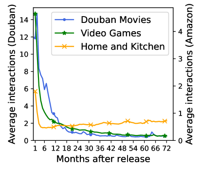
(a)

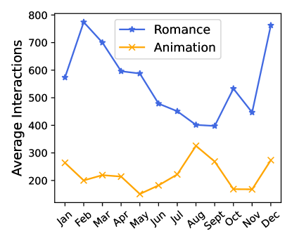
(b)

Figure 1. (a) Average monthly interactions of items after being released on three datasets. Douban Movies is from Douban. Both Home and Kitchen and Video Games are from Amazon. (b) Average monthly interactions for movies within the Romance and Animation genres on Douban Movies.

2. Related Works

2.1. Sequential Recommendation

Traditional recommendation methods often assign equal importance to all historical user-item interactions, overlooking the reality that user preferences and the appeal of items can change over time (He and McAuley, 2016a; Rendle et al., 2010; He et al., 2017a). Furthermore, recognizing sequential dependencies in user behaviors, such as purchasing car insurance after buying a car, can enrich the system’s understanding of the user’s actions. Therefore, sequential recommendation systems are introduced to capture the evolution of user preferences, which places a greater emphasis on recent interactions (Ma et al., 2019; Tang and Wang, 2018; Li et al., 2019; Liu et al., 2018).

Early sequential recommendation methods model the sequential patterns with Markov Chain (MC) (Rendle et al., 2010; He and McAuley, 2016a; He et al., 2016) or translation-based models (He et al., 2017a; Li et al., 2019). Rendle et al. (2010) combined the first-order MC and matrix factorization to model the sequential information and make predictions, achieving admirable results. He and McAuley (2016a) further introduced high-order MC to extract more complicated information to make personalized recommendations. He et al. (2017a) proposed a Translation-based model, TransRec, which focuses on user-item-item third-order relationship.

Later, deep neural network approaches have been integrated into sequential recommendation systems. It is intuitive to utilize recurrent neural networks (RNNs) due to their capability to effectively process sequential inputs (Hidasi et al., 2015, 2016; Donkers et al., 2017; Quadrana et al., 2017; Ma et al., 2019; Yu et al., 2016). RNN-based sequential recommendation systems usually leverage long-short-term-memory (LSTM) or gated recurrent units (GRU) to capture sequential dependencies (Donkers et al., 2017; Zhu et al., 2017; Hidasi et al., 2015; Zheng et al., 2019). However, these RNN-based models heavily depend on interaction sequences and are tailored to model point-wise dependencies, potentially overlooking collective dependencies (Kang and McAuley, 2018; Sun et al., 2019). Additionally, convolution neural networks (CNN) are also applied in sequential recommendation systems (Tang and Wang, 2018; Jiang et al., 2022). These systems first regard sequential interaction as a matrix and subsequently treat this matrix as an ”image” in both temporal and latent spaces (Tang and Wang, 2018). In recent years, graph neural networks (GNN) have emerged as a leading approach in sequential recommendation systems (Wu et al., 2019; Zhang et al., 2020; Xu et al., 2019) and the attention mechanism has demonstrated significant promise in the sequential recommendation (Li et al., 2017; Liu et al., 2018; Kang and McAuley, 2018; Fan et al., 2022). For example, to model both global and local information on the graph, Xu et al. (2019) dynamically constructed a graph with a self-attention mechanism for session sequences.

Summary: Sequential recommendation systems are designed to capture the change in users’ preferences by assigning varying levels of importance to historical user-item interactions. However, to the best of our knowledge, all the existing sequential recommendation approaches fail to model the fluctuations in item popularity over time, which are crucial for influencing users’ decisions.

2.2. Item Popularity in Recommender Systems

It is intuitive to make recommendations based on the items’ popularity. The non-personalized strategy, which consistently recommends the most popular items according to the whole interaction history, has often been employed as a benchmark in assessing recommendation systems (Ji et al., 2020; Tang and Wang, 2018; Kang and McAuley, 2018; He et al., 2017b). Also, item popularity has been discussed extensively in relation to recommendation systems.

First, the so-called ”long-tail” phenomenon presents a significant challenge. In this scenario, a small fraction of items gain immense popularity and attract a large user base, while a majority of items are consumed by very few users (Abdollahpouri et al., 2019; Abdollahpouri and Mansoury, 2020), which may lead the recommendation system to over-recommend popular items. Various methods have been proposed to address such problems, including regularization models (Abdollahpouri et al., 2017; Chen et al., 2020; Kamishima et al., 2014; Zhu et al., 2021), Causal-based models (Wang et al., 2021; Wei et al., 2021; Zhang et al., 2021; Zheng et al., 2021a), and adversarial models (Krishnan et al., 2018; Arduini et al., 2020). Regularization models directly regulate the model predictions according to item popularity (Zhu et al., 2021; Kamishima et al., 2014; Abdollahpouri et al., 2017) or placing more emphasis on unpopular items (Chen et al., 2020). On the other hand, causal-based methods apply counterfactual intervention over the Causal Graph (Peters et al., 2017) to mitigate the bias. Lastly, adversarial models try to strike a balance between recommending less popular items and using existing knowledge to maintain recommendation accuracy (Krishnan et al., 2018; Arduini et al., 2020). However, removing popularity bias directly usually negatively impacts the accuracy of the recommendations. As a result, recent studies have been focusing on reducing popularity bias while maintaining the models’ performances (Zhao et al., 2022; Xv et al., 2022; Yang et al., 2023).

Moreover, researchers have studied the effects of different methods of calculating item popularity on recommendation performance. Ji et al. (2020) compared the perofmances of the MostPop, RecentPop, and DecayPop models. The MostPop model recommends items with the highest global popularity, while RecentPop recommends the most popular movies from the past month. The DecayPop model, on the other hand, accounts for the weighted sum of an item’s popularity over the past six months. The results showed that both RecentPop and DecayPop outperformed the traditionally used MostPop model, suggesting that recent item popularity influences user choices more than overall item popularity throughout the entire interaction history. In another study, Anelli et al. (2019) proposed TimePop to track item popularity within a user’s specific network and make recommendations based on this personalized item popularity.

Summary: Despite a wealth of research on item popularity in recommendation systems, there’s a gap when it comes to explicitly predicting an item’s future popularity trend. Furthermore, current research focuses on the interactions between users and items, often underestimating the influence of item popularity trends on the recommendation system.

3. Popularity-Aware Recommender

3.1. Problem Definition

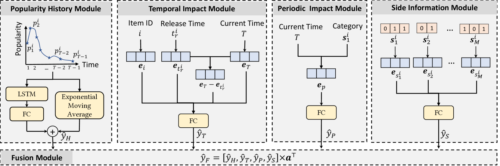
Figure 2. The proposed architecture of PARE. The model consists of four modules modeling popularity history, temporal impact, periodic impact, and side information, respectively. Finally, an attention layer is leveraged to fuse the outputs of four modules.

We first present essential notations. We use $i\in\mathcal{I}$ to denote the item and $t\in\mathcal{T}$ to denote the time. Each item $i$ is associated with multiple features, such as the release time $t^{i}_{r}$ and $M$ other side information $\mathcal{S}^{i}=\{s^{i}_{1},\cdots,s^{i}_{M}\}$. Note that $\mathbf{s}^{i}_{1}\in\mathbb{R}^{C}$ refers to the item category, whereas $C$ refers to the number of categories. If item $i$ is associated with category $j$, $\mathbf{s}^{i}_{1}[j]=1$, otherwise, $\mathbf{s}^{i}_{1}[j]=0$. Also, the time $t$ is not a single timestamp but a period of time, so item $i$ may have multiple interactions at time $t$. We denote the set of users who have interacted with item $i$ at time $t$ as $\mathcal{U}^{i}_{t}=\{u^{i}_{1},\cdots,u^{i}_{|\mathcal{U}^{i}_{t}|}\}$, where $|\cdot|$ denotes the set size. The popularity of $i$ is then defined as $p^{i}_{t}=|{\mathcal{U}^{i}_{t}}|$, where $t\geq t^{i}_{r}$.

Given the item release time $t^{i}_{r}\in\mathcal{T}$, the popularity history $\mathbf{p}^{i}=[p^{i}_{t^{i}_{r}},\cdots,p^{i}_{T-2},p^{i}_{T-1}]$, and other side information $\mathcal{S}^{i}$ of item $i$, the goal is to predict the item popularity $p^{i}_{T}$ at time $T$. Then the top $N$ items with the highest predicted popularity will be recommended to all users without distinction.

3.2. Model Architecture

As shown in Figure 2, PARE consists of four concise modules, each designed to predict the impending item popularity from distinct facets of item attributes. Finally, a Fusion Module combines the four predictions using an attention layer.

3.2.1. Popularity History Module

The past popularity of an item can usually provide a reasonable approximation of its current popularity. We believe that an item’s popularity generally follows specific trends based on its current popularity and rarely experiences sudden, drastic shifts over time. Therefore, as shown in Figure 2, we incorporated two simple but effective components into PARE, which are designed to assess the item’s latest popularity status and predict the impending popularity trend, respectively.

First, given the presumption that recent popularity carries more significance than older popularity, we utilize the exponential moving average (EMA) (Klinker, 2011) method, which assigns a higher weight to more recent data points. We use $\text{EMA}_{t}^{i}$ to denote the popularity estimator for item $i$ at time $t$:

(1) $$\text{EMA}_{t}^{i}=\left\{\begin{array}[]{ccl}0&&\text{if}\ t<t^{i}_{r}\\ p^{i}_{t^{i}_{r}}&&\text{if}\ t=t^{i}_{r},\\ \alpha p^{i}_{t}+(1-\alpha)\text{EMA}_{t-1}^{i}&&else\end{array}\right.$$

where $\alpha\in[0,1]$. A higher value of $\alpha$ refers to a greater emphasis on the recent popularity of the item. The latest popularity status at current time $T$ is then defined as $\hat{y}_{status}=\text{EMA}_{T-1}$.

Then, in order to predict whether an item will gain increased attention or decline in popularity, we utilize the Long Short-Term Memory (LSTM) method (Sak et al., 2014). The distinctive use of a cell state and gating mechanisms in LSTMs allows them to selectively remember or forget information across various time intervals, rendering them particularly suitable for tasks involving long sequences. More specifically, given the popularity history $\mathbf{p}^{i}=[p^{i}_{t^{i}_{r}},\cdots,p^{i}_{T-2},p^{i}_{T-1}]$, the following operations are carried out:

(2) $$\begin{split}I_{t}&=\sigma(\textbf{W}_{I}[p_{t}^{i},H_{t-1}]+\textbf{b}_{I})\\ F_{t}&=\sigma(\textbf{W}_{F}[p_{t}^{i},H_{t-1}]+\textbf{b}_{F})\\ G_{t}&=\text{tanh}(\textbf{W}_{G}[p_{t}^{i},H_{t-1}]+\textbf{b}_{G})\\ O_{t}&=\sigma(\textbf{W}_{O}[p_{t}^{i},H_{t-1}]+\textbf{b}_{O})\\ C_{t}&=F_{t}\odot C_{t-1}+I_{t}\odot G_{t}\\ H_{t}&=O_{t}\odot\text{tanh}(C_{t}),\end{split}$$

where $H_{t}$, and $C_{t}$ represent the hidden state and cell state of the popularity at time $t$. $I_{t}$, $F_{t}$, $G_{t}$, and $O_{t}$ denote the input, forget, cell, and output gates, respectively. $\sigma$ denotes a sigmoid layer that maps the values between 0 and 1, with 1 meaning retaining the whole information and 0 signifying discarding it entirely. The operation $\odot$ denotes the Hadamard product. The final hidden state, $H_{T-1}$, is then fed into a fully connected layer to predict the popularity trend:

(3) $$\hat{y}_{trend}=\bm{w}_{H}^{\top}H_{T-1}+\bm{b}_{H}.$$

In this case, a positive $\hat{y}_{trend}$ suggests an increase in popularity, while a negative value indicates a decrease.

Finally, we combine the two estimations using:

(4) $$\hat{y}_{H}=\hat{y}_{status}+\hat{y}_{trend}.$$

3.2.2. Temporal Impact Module

As illustrated in Figure 1a, we notice that peak attention typically occurs within the first two months after the item’s release. Generally, as the temporal distance from the item’s release increases, the item tends to diminish in popularity. The duration for which an item can maintain its popularity is significantly tied to the item itself. In this module, PARE captures the influence of temporal factors on the item’s popularity.

First, the current time $T$ and item release time $t_{r}^{i}$ are embedded, yielding $\mathbf{e}_{T}\in\mathbb{R}^{d}$ and $\mathbf{e}_{t_{r}^{i}}\in\mathbb{R}^{d}$, respectively. $d$ refers to the embedding size. Note that both times share the same embedding space. Given the significant role of temporal distance in popularity prediction, we define $\mathbf{e}_{dis}=\mathbf{e}_{T}-\mathbf{e}_{t_{r}^{i}}$. Then we concatenate $\mathbf{e}_{T}$, $\mathbf{e}_{t_{r}^{i}}$, $\mathbf{e}_{dis}$, along with the item embedding $\mathbf{e}_{i}\in\mathbb{R}^{d}$. Finally, the concatenation is fed into a fully connected layer to predict the item popularity:

(5) $$\begin{split}\hat{y}_{T}&=\text{ReLU}(\bm{w}_{T}^{\top}[\mathbf{e}_{T},\mathbf{e}_{t_{r}^{i}},\mathbf{e}_{dis},\mathbf{e}_{i}]+\bm{b}_{T}).\end{split}$$

3.2.3. Periodic Impact Module

Besides the temporal evolution of item popularity, we also observe periodic fluctuations in the popularity of different categories of items over time. As shown in Figure 1b, movies from Romance and Animation undergo periods of surges and declines in different months. This phenomenon is not exclusive to movies and can be seen across various items. For instance, T-shirts see increased popularity during summer, whereas sweaters gain popularity during winter.

To capture this periodic effect, we construct an embedding matrix $\mathbf{E}\in\mathbb{R}^{(\omega C)\times d}$, where $\omega$ represents period time. For example, if each $t$ refers to one month and $\omega=12$, it suggests that categories of an item follow similar popularity trends annually. Given the current time $T$, we first transform to a one-hot vector $\mathbf{v}_{T}\in\{0,1\}^{\omega}$. If time $T$ falls within the $j^{th}$ period, then $\mathbf{v}_{T}[j]=1$, otherwise, $\mathbf{v}_{T}[j]=0$. Then we calculate the periodic embedding using the item categories $\mathbf{s}^{i}_{1}\in\mathbb{R}^{C}$ and time $\mathbf{v}_{T}$:

(6) $$\begin{split}\mathbf{e}_{p}&=\left[\text{Flatten}\left(\left(\mathbf{s}^{i}_{1}\right)^{\top}\times\mathbf{v}_{T}\right)\right]\times\mathbf{E}.\end{split}$$

Finally, we feed the embedding into a fully connected layer, which is activated by ReLU:

(7) $$\hat{y}_{P}=\text{ReLU}(\bm{w}_{P}^{\top}\bm{e}_{p}+\bm{b}_{P}).$$

3.2.4. Side Information Module

Incorporating side information substantially enhances the accuracy of item popularity predictions. First, item’s side information is closely related to the peak popularity and duration of popularity. Taking movies as an example, a movie produced by more famous directors or actors usually tends to attract a larger audience and stay popular for a longer period of time. Furthermore, side information can be particularly useful when dealing with cold-start items that have little or even no popularity history. For each kind of side information $\mathbf{s}_{j}\in\{0,1\}^{q_{j}}$, where $j\leq M$ and $q_{j}$ is the number of attributes for $j$, we feed them into an embedding layer:

(8) $$\mathbf{e}_{s_{j}^{i}}=\mathbf{s}^{i}_{j}\times\mathbf{E}_{j},$$

where $\mathbf{E}_{j}\in\mathbb{R}^{q_{j}\times d}$. Finally, we concatenate the $M$ kinds of side information and utilize a fully connected later to predict how the side information influences the item popularity:

(9) $$\hat{y}_{S}=\text{ReLU}(\bm{w}_{S}^{\top}[\mathbf{e}_{s_{1}^{i}},\mathbf{e}_{s_{2}^{i}},\cdots,\mathbf{e}_{s_{M}^{i}}]+\bm{b}_{S}).$$

3.2.5. Module fusion

In this module, we combine the four predictions with a simple 4-dimensional attention vector $\bm{a}\in\mathbb{R}^{4}$:

(10) $$\hat{y}_{F}=[\hat{y}_{H},\hat{y}_{T},\hat{y}_{P},\hat{y}_{S}]\times\bm{a}^{\top}$$

subject to the condition $\sum\mathbf{a}=1$. Through the attention layer, PARE can incorporate all model factors, including item popularity history, temporal effects, periodic effects, and side information. Furthermore, the attention layer enhances interpretability by demonstrating how the four modules contribute to the final prediction.

3.3. Training

Since the predicted output from each module is expected to closely align with the actual item popularity, we employ the mean square error (MSE) loss from each module to train the model as follows:

(11) $$\begin{split}\mathcal{L}=\sum_{j\in\{H,T,P,S,F\}}\mathbb{E}_{i\in\mathcal{I},t<T}\left[\left(p^{i}_{t}-\hat{y}_{j}\right)^{2}\right],\\ \end{split}$$

where $p^{i}_{t}$ represents the actual popularity of item $i$ at time $t$, while $\hat{y}_{j}$ denotes the predicted popularity for item $i$ at time $t$, as generated by module $j$. We use Adam (Kingma and Ba, 2015) for model optimization.

4. Experimental Settings

4.1. Datasets

The proposed PARE is evaluated on three real-world datasets: Douban Movies, Video Games, and Home and Kitchen. The Douban Movies dataset is crawled from the Douban website1, which is one of the largest Chinese social media sites that allow users to make comments on movies, books, music, etc. We crawl all movies that are released from 1^st January 2011 to 31^st December 2020 and their side information including categories, directors, and actors. Moreover, Douban Movies consists of all user-item interactions where the user has commented on the item during the same time period. In summary, Douban Movies comprises 33,635 users and 2,795 movies. Further evaluation is conducted using two public datasets from Amazon(He and McAuley, 2016b): Video Games and Home and Kitchen. More statistics are summarized in Table 1.

It is worth noting that we use a fixed global time-point to split the dataset into training, validation, and testing sets. This splitting effectively prevents information leakage and more closely resembles real-world scenarios compared to commonly used strategies such as the Leave-One-Last or Temporal-User-Split (Campos et al., 2011; Meng et al., 2020). In our experiments, we define each time $t$ as a 30-day period, with $t=1$ representing the first 30 days subsequent to the first user-item interaction in the whole dataset. The interactions from the final month are used for testing, those from the penultimate month are used for validation, and all remaining interactions are used for training. It’s important to note that the time period in the test set may be less than one month, resulting in a relatively small number of interactions.

Table 1. Statistics of the datasets.

Dataset	#Users	#Items	#Train	#Validate	#Test
Douban Movies	33,635	2,795	329,380	1,992	560
Video Games	23,933	4,211	169,845	1,968	1,977
Home and Kitchen	65,588	8,633	361,005	13,448	376

4.2. Baselines

Table 2. Model performances of Top-10 recommendation. The best results among variants of Cutoff TopPop are marked with ^∗. The best results and the second-best results within each group are bold and underlined, respectively. Relative Imp-1. denotes to the improvement of PARE over the best original baselines, Relative Imp-2 denotes the improvement of integrated model over PARE.

Methods		Douban Movies					Video Games					Home and Kitchen
		Precision	Recall	HR	MRR	NDCG	Precision	Recall	HR	MRR	NDCG	Precision	Recall	HR	MRR	NDCG
Cutoff TopPop	3 months	0.0177∗	0.1460∗	0.1742∗	0.0062∗	0.0661∗	0.0086	0.0565	0.0833	0.0039	0.0285∗	0.0039∗	0.0370∗	0.0391 ∗	0.0036∗	0.0335∗
	6 months	0.0118	0.0822	0.1124	0.0045	0.0387	0.0092	0.0567∗	0.0877	0.0041∗	0.0283	0.0004	0.0043	0.0043	0.0002	0.0027
	12 months	0.0115	0.0796	0.1096	0.0032	0.0316	0.0094∗	0.0545	0.0892 ∗	0.0040	0.0274	0.0000	0.0000	0.0000	0.0000	0.0000
	ALL	0.0042	0.0306	0.0421	0.0012	0.0119	0.0069	0.0391	0.0643	0.0036	0.0218	0.0000	0.0000	0.0000	0.0000	0.0000
Original	UserKNN	0.0048	0.0345	0.0449	0.0016	0.0143	0.0127	0.0809	0.1155	0.0044	0.0359	0.0048	0.0384	0.0478	0.0015	0.0174
	ItemKNN	0.0039	0.0252	0.0337	0.0015	0.0110	0.0121	0.0763	0.1097	0.0042	0.0338	0.0043	0.0370	0.0435	0.0018	0.0193
	SLIM BPR	0.0051	0.0360	0.0506	0.0018	0.0159	0.0117	0.0706	0.1067	0.0044	0.0326	0.0043	0.0391	0.0435	0.0014	0.0177
	NCF	0.0045	0.0318	0.0421	0.0014	0.0118	0.0066	0.0377	0.0599	0.0033	0.0198	0.0026	0.0217	0.0261	0.0007	0.0094
	SHT	0.0059	0.0364	0.0590	0.0028	0.0193	0.0102	0.0600	0.0921	0.0039	0.0291	0.0022	0.0217	0.0217	0.0007	0.0100
	Caser	0.0048	0.0339	0.0478	0.0010	0.0116	0.0089	0.0620	0.0863	0.0026	0.0248	0.0043	0.0362	0.0435	0.0010	0.0147
	SASRec	0.0098	0.0691	0.0955	0.0037	0.0336	0.0089	0.0497	0.0863	0.0043	0.0269	0.0035	0.0326	0.0348	0.0017	0.0195
	HGN	0.0104	0.0713	0.0983	0.0041	0.0345	0.0151	0.1005	0.1389	0.0053	0.0465	0.0074	0.0667	0.0696	0.0019	0.0277
	STOSA	0.0124	0.0870	0.1208	0.0062	0.0484	0.0148	0.0941	0.1404	0.0053	0.0425	0.0074	0.0623	0.0739	0.0031	0.0323
	ICLRec	0.0135	0.0961	0.1236	0.0054	0.0456	0.0178	0.1125	0.1667	0.0056	0.0430	0.0070	0.0623	0.0696	0.0024	0.0279
	PARE	0.0208	0.1695	0.1994	0.0092	0.0955	0.0104	0.0647	0.0950	0.0042	0.0300	0.0074	0.0674	0.0696	0.0054	0.0527
Relative Imp-1.		54.17%	76.46%	61.36%	47.64%	97.24%	-41.80%	-42.51%	-42.98%	-25.42%	-35.59%	0.00%	1.09%	-5.88%	74.56%	62.80%
+PARE	UserKNN	0.0208	0.1688	0.2023	0.0092	0.0946	0.0154	0.0922	0.1418	0.0056	0.0439	0.0091	0.0804	0.0826	0.0054	0.0540
	ItemKNN	0.0225	0.1716	0.2079	0.0084	0.0833	0.0155	0.0994	0.1433	0.0052	0.0420	0.0091	0.0804	0.0826	0.0056	0.0558
	SLIM BPR	0.0211	0.1716	0.2051	0.0086	0.0927	0.0149	0.0945	0.1374	0.0055	0.0425	0.0087	0.0783	0.0826	0.0053	0.0529
	NCF	0.0219	0.1702	0.2079	0.0085	0.0859	0.0096	0.0595	0.0921	0.0041	0.0284	0.0083	0.0761	0.0783	0.0044	0.0474
	SHT	0.0216	0.1735	0.2107	0.0085	0.0798	0.0140	0.0814	0.1272	0.0050	0.0362	0.0083	0.0761	0.0783	0.0041	0.0451
	Caser	0.0213	0.1721	0.2135	0.0073	0.0785	0.0116	0.0703	0.1067	0.0042	0.0309	0.0117	0.1109	0.1130	0.0053	0.0613
	SASRec	0.0225	0.1751	0.2163	0.0074	0.0772	0.0111	0.0659	0.1038	0.0045	0.0308	0.0074	0.0674	0.0696	0.0057	0.0543
	HGN	0.0236	0.1819	0.2247	0.0087	0.0858	0.0181	0.1151	0.1725	0.0059	0.0493	0.0135	0.1239	0.1261	0.0057	0.0657
	STOSA	0.0222	0.1730	0.2135	0.0080	0.0807	0.0151	0.1001	0.1433	0.0055	0.0453	0.0148	0.1348	0.1391	0.0069	0.0776
	ICLRec	0.0208	0.1695	0.1994	0.0094	0.0970	0.0194	0.1205	0.1813	0.0068	0.0508	0.0122	0.1080	0.1130	0.0056	0.0618
Relative Imp-2.		13.51%	7.32%	12.68%	2.52%	1.54%	87.32%	86.32%	90.77%	63.21%	69.52%	100.01%	100.00%	100.00%	27.46%	47.38%

We select the following methods for evaluation, including traditional methods, non-sequential recommendation methods, and sequential recommendation methods. We use the published codes for implementing baseline methods.

• Cutoff TopPop, which recommends the items that are most popular during a specific time period. Cutoff TopPop – ALL is one of the most widely used recommendation baselines that always recommend the most popular item based on the entire history of user-item interactions. Inspired by Ji et al. (2020), we also incorporate variations of TopPop that calculate popularity using recent interaction data. In our experiments, we consider recent interactions in the last 3 months, 6 months, and 12 months.

• UserKNN (Sarwar et al., 2001; Dacrema et al., 2019), a traditional collaborative filtering method based on the k-nearest neighbors algorithm. Using the validation set, we select the best from five distance functions for user-user similarity, including cosine, Jaccard, Dice, Tversky, and asymmetric distances.

• ItemKNN3 (Wang et al., 2006), a neighborhood-based method using collaborative item-item similarity. We tune the selection of the distance functions in the same manner as UserKNN.

• SLIM BPR3 (Ning and Karypis, 2011), which leverages a sparse coefficient matrix to predict user behaviors and is optimized with Bayesian Personalized Ranking (BPR) loss.

• NCF (He et al., 2017b), which is a non-sequential baseline that combines a generalized matrix factorization module and a multi-layer perceptron.

• SHT (Xia et al., 2022), which is a non-sequential baseline that replaces the dot-product in conventional matrix factorization with a hypergraph transformer network and conducts data augmentation with a generative self-supervised learning component.

• Caser (Tang and Wang, 2018), which is a CNN-based method that applies horizontal and vertical convolutions for sequential recommendation.

• SASRec (Kang and McAuley, 2018), which is a self-attention-based sequential model which utilizes an attention mechanism.

• HGN (Ma et al., 2019), which captures both user intents and item-item relations from item sequences with a hierarchical gating network.

• STOSA (Fan et al., 2022), which embeds each item as a stochastic Gaussian distribution, and forecasts the next item for sequential recommendation with a self-attention mechanism.

• ICLRec (Chen et al., 2022), which learns users’ preferences from unlabeled user historical interactions and is optimized through contrastive self-supervised learning.

4.3. Evaluation Metrics

To evaluate the performance of Top-N recommendations, we use the hit ratio (HR), precision, recall, mean reciprocal rank (MRR), and normalized discounted cumulative gain (NDCG) for N = 1,3,5,7,10. The HR, precision, and recall metrics measure whether and how many of the target item appears in the top-N list, whereas the MRR and NDCG consider the ranking position of target items within the list.

4.4. Method Integration

To demonstrate the efficacy of the PARE as a complementary component to existing recommendation methods, we propose to incorporate the item popularity score, as predicted by our model, with the estimated user preferences for items in existing recommendation methods. More specifically, if $\hat{y}_{F}$ represents the predicted item popularity for item $i$ at time $T$, $s(u,i)$ represents the predicted preference score for user $u$ regarding item $i$, with a higher $s(u,i)$ indicating a greater likelihood for the user to select the item. Then the updated ranking score at a specific time $T$ can be formulated as follows:

(12) $$s_{new}(u,i,T)=\beta s(u,i)+(1-\beta)\hat{y}_{F},$$

where $\beta$ serves as a hyperparameter that regulates the balance between the influence of item popularity and user personalization in user decisions. A lower value of $\beta$ indicates that user choices are more influenced by the current item popularity, while a higher $\beta$ emphasizes more on the importance of personalized recommendations.

4.5. Implementation Details

In our experiments, we select learning rate from $[0.0001,0.1]$ and batch size from $\{64,128,256\}$. We also apply L2 regularization when computing the loss function in Equation 11 with the weight decay being $0.0001$. The embedding size $d$ is set to 64.

5. Results and Discussion

We first compare the performances between different recommendation models as well as their variants integrated with PARE. We also carry out a comprehensive ablation study to assess the effectiveness of each module within our proposed PARE, the accuracy of item popularity prediction, as well as the efficacy of our model when used as a complementary component alongside existing recommendation baselines.

Table 3. Model performances with different Top-N value of hit ratio (HR) on Douban Movies. The best results among variants of Cutoff TopPop are marked with ^∗. The best results and the second-best results within each group are bold and underlined, respectively. Relative Imp-1. denotes to the improvement of PARE over the best original baselines, Relative Imp-2 denotes the improvement of integrated model over PARE.

Methods		@1	@3	@5	@7
Cutoff TopPop	3 months	0.0337∗	0.0534	0.0646	0.1320∗
	6 months	0.0112	0.0674∗	0.0927∗	0.0955
	12 months	0.0056	0.0506	0.0590	0.0843
	ALL	0.0056	0.0112	0.0112	0.0309
Original	UserKNN	0.0028	0.0197	0.0309	0.0393
	ItemKNN	0.0084	0.0140	0.0253	0.0253
	SLIM BPR	0.0112	0.0169	0.0197	0.0281
	NCF	0.0056	0.0169	0.0281	0.0337
	SHT	0.0169	0.0309	0.0393	0.0478
	Caser	0.0000	0.0084	0.0253	0.0309
	SASRec	0.0169	0.0449	0.0646	0.0646
	HGN	0.0225	0.0421	0.0702	0.0787
	STOSA	0.0393	0.0702	0.0983	0.1039
	ICLRec	0.0253	0.0702	0.0899	0.1067
	PARE	0.0534	0.0927	0.1461	0.1629
Relative Imp-1.		35.71%	32.00%	48.57%	52.63%
+ PARE	UserKNN	0.0309	0.1264	0.1433	0.1714
	ItemKNN	0.0337	0.1124	0.1629	0.1770
	SLIM BPR	0.0225	0.1208	0.1517	0.1685
	NCF	0.0562	0.1124	0.1461	0.1685
	SHT	0.0309	0.1152	0.1545	0.1685
	Caser	0.0281	0.0843	0.1433	0.1742
	SASRec	0.0225	0.0871	0.1601	0.1798
	HGN	0.0365	0.1152	0.1685	0.1910
	STOSA	0.0253	0.1096	0.1573	0.1714
	ICLRec	0.0337	0.1039	0.1629	0.1938
Relative Imp-2.		5.26%	36.36%	15.38%	18.97%

5.1. Recommendation Performances

Due to space constraints, we present the model performance for the top 10 recommendations, as assessed by all evaluation metrics, across the three datasets in Table 2. Besides, the hit ratio performance with varying top $N$ values on the Douban Movies dataset is shown in Table 3. From these results, we make the following observations.

First, our findings align with those of Ji et al. (2020), wherein recommending items based solely on recent popularity outperforms the commonly used Cutoff TopPop - ALL baseline on all datasets in terms of all metrics. The latter always recommends the most popular item according to the entire interaction history. On the Douban Movies dataset, the MRR@10 and NDCG@10 for Cutoff TopPop - 3 months are more than four times greater than those for making recommendations considering all data. Besides, we also find that the best variant of Cutoff TopPop outperforms most recommendation baselines on Douban Movies. These results underline the significant influence of recent item popularity on user decision-making. Moreover, these findings inspire us to consider utilizing Cutoff TopPop over a short time span, rather than the generally adopted Cutoff TopPop - ALL, as a solid baseline for evaluating future recommendation models.

Second, the simple non-personalized PARE performs at a similar level or even surpasses the more complex state-of-the-art recommendation methods. On Douban Movies, PARE outperforms the best baseline by $97.24\%$ and $76.46\%$ in NDCG@10 and Recall@10, respectively. However, we observed that PARE performs relatively less effectively on the Video Games dataset, where the personalized sequential recommendation baseline ICLRec exhibits the best performance. This could be attributed to the diverse tastes of users in video games, who tend to purchase based on their personal preferences rather than opting for the most popular choices. Considering these findings, our model could serve as a strong baseline for future recommendation evaluations and assist in analyzing the impact of both user preference and item popularity on user decision-making.

Third, when we integrate our proposed PARE into existing recommendation methods using Equation 12, the combined model outperforms all corresponding original personalized recommendation baselines. We observe a relatively significant improvement over the original existing baselines on the Douban Movies dataset and a more pronounced enhancement over PARE on the other two datasets. On Douban Movies, the combined ItemKNN+PARE improves the original ItemKNN by approximately 7 times in HR@3, however, it only enhances the original PARE model by only about $21\%$. On Home and Kitchen, we observe a doubling of performance when we incorporate existing recommendation baselines into our model in terms of precision, recall, and HR for the top 10 recommendations.

In summary, these experimental findings demonstrate the effectiveness of our proposed model both as a strong baseline for future research and as a potential complementary component capable of enhancing the performance of existing recommendation methods.

5.2. Effectiveness of Each Module

Table 4. Comparison of each module on Douban Movies. H, T, P, and S denote the Popularity History Module, Temporal Impact Module, Side Information Model, and Periodic Impact Module, respectively. ”Attention Weight” denotes the corresponding attention score in the Fusion Module.

Metric	HR@10	Attention Weight
		H	T	S	P
H	0.1798	1.0000	-	-	-
H+T	0.1910	0.6025	0.3975	-	-
H+T+S	0.1938	0.6070	0.2047	0.1882	-
H+T+P	0.1966	0.5980	0.1844	-	0.2177
H+T+S+P	0.1994	0.6259	0.2573	0.0422	0.0746

Comparing the variants of Cutoff TopPop with PARE, as seen in Table 2 and Table 3, we found that PARE consistently outperforms Cutoff TopPop across all metrics and datasets. This suggests that item popularity history is not the sole determinant of user decisions; additional item side information, such as categories and release times, are also key factors. To further explore the efficacy of each module, we compared the performance of recommendations when different module combinations were applied on Douban Movies.

We illustrate the comparison results in Table 4, where H, T, S, and P denote the Popularity History Module, Temporal Impact Module, Side Information Model, and Periodic Impact Module, respectively. The “Attention Weight” refers to the corresponding attention score described in Equation 10. From the results in Table 4, we notice that the most effective combination incorporates all four modules, thereby demonstrating their collective contributions to the high-performance recommendations delivered by PARE. According to the attention weight, the Popularity History Module holds the highest importance, followed by the Temporal Impact Module. Considering that our experiments on the Douban Movies dataset only include attributes like categories, directors, and actors, we believe the influence of side information could potentially be enhanced if we integrate further details, such as user comments about the movies.

5.3. Performances of Item Popularity Prediction

Table 5. Performance of two leading baseline models and their variants integrated with PARE and Groundtruth for Top-10 recommendation on Douban Movies. Groundtruth recommends the item with the highest actual popularity.

Methods		Precision	Recall	HR	MRR	NDCG
PARE		0.0208	0.1695	0.1994	0.0092	0.0955
Groundtruth		0.0360	0.3025	0.3371	0.0155	0.1666
STOSA	Original	0.0124	0.0870	0.1208	0.0062	0.0484
	+PARE	0.0222	0.1730	0.2135	0.0080	0.0807
	+Groundtruth	0.0365	0.3032	0.3399	0.0154	0.1644
ICLRec	Original	0.0135	0.0961	0.1236	0.0054	0.0456
	+PARE	0.0208	0.1695	0.1994	0.0094	0.0970
	+Groundtruth	0.0376	0.3153	0.3567	0.0165	0.1752

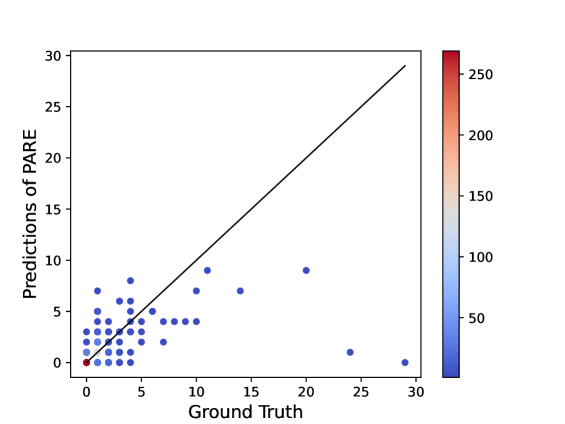
(a) Distribution of items based on their predicted popularity scores and their actual (Ground Truth) popularity. The color of each data point indicates the number of items at that point.

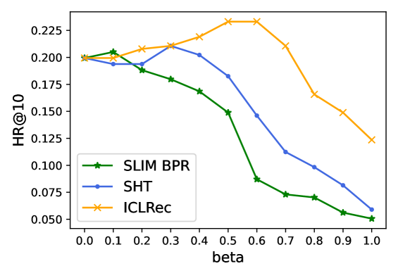
(b) HR@10 comparison of 3 baseline models when integrated with PARE through different $\beta$ on Douban Movies.

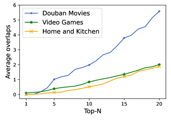
(c) The number of overlapping items between the prediction list of PARE and ICLRec on three datasets at varies Top-N recommendations.

Figure 3. Ablation Study

In this experiment, we first analyze the accuracy of PARE in predicting item popularity. Figure 3a presents a visualization of the number of items as plotted against the predicted popularity and the actual popularity score from the test set of Douban Movies. Alongside this, we also display a randomly selected equivalent number of items that are absent from the test set for comparison. We made the following observations. Firstly, for all items lacking interactions within the test set, the predicted popularity of these items does not exceed 3, highlighting the reasonable accuracy of PARE when predicting for negative samples. Second, the predicted popularity of a significant portion of positive samples aligns closely with, or falls within 5 units of, the actual popularity, barring a few outliers. According to these experimental results, PARE can accurately predict item popularity to a certain extent.

Then, we aim to understand the upper-bound performance of non-personalized recommendation methods that solely rely on item popularity. To this end, we compare the performance of the top 10 recommendations generated by PARE model with those recommending the item having the highest ground-truth popularity, represented as Groundtruth, on Douban Movies. Moreover, We evaluate the variants of two leading baseline models (i.e., STOSA and ICLRec), including the original approach, and versions integrated with PARE and Groundtruth. As illustrated in Table 5, Groundtruth surpasses PARE by 78.43% and 74.47% in Recall@10 and NDCG@10, respectively, indicating potential room for improvement. Upon comparing the three variants of STOSA and ICLRec, it’s evident that the original method lags behind in performance, while the version integrated with Groundtruth significantly outperforms the other two variants. These insights further underscore the efficacy of taking item popularity into account when making recommendations.

5.4. Effectiveness of PARE as a Complementary Component

To evaluate the effectiveness of PARE when used as a complementary component to existing recommendation methods, we perform two ablation studies. First, as shown in Figure 3b, we compare the HR@10 on Douban Movies of varying $\beta$ values in Equation 12 when PARE is integrated with the best-performing recommendation baseline methods from traditional, non-sequential, and sequential methods, these being SLIM BPR, SHT, and ICLRec, respectively. We observed that the integrated model with ICLRec exhibits superior performance when $\beta=0.6$. For SHT and SLIM BPR, the optimal performances were achieved at $\beta=0.3$ and $\beta=0.1$. As illustrated in Table 2, ICLRec outperformed the other two baselines, followed by SHT and SLIM BPR. These findings suggest that when the personalized recommendation model is not as strong, a lower $\beta$ value allows the integrated model to perform better, likely due to the increased emphasis on item popularity.

Then, we analyze the number of items that overlap between the recommendation list generated by PARE and existing recommendation methods across three datasets. As depicted in Figure 3c, we observe that the quantity of overlapping items increases approximately linearly as the number of items in the recommendation list grows. However, the absolute count of overlapping items remains relatively small, with approximately 2 items on Video Games and Home and Kitchen when recommending 20 items. This observation corroborates our assumption that due to the distinct approach of PARE which doesn’t rely on historical user-item interactions, it would yield a smaller overlap in the recommendation list compared to existing methods based on collaborative filtering.

In summary, these ablation studies show the benefits of integrating PARE into existing recommendation models. Besides, these findings emphasize that when the original recommendation algorithm is deficient in effectiveness, the performance exhibits a more significant improvement upon integration with PARE.

6. Conclusion

In conclusion, this paper has shed light on the critical influence of temporal fluctuations in item popularity for recommender systems. We identified that most existing recommendation methods focus on understanding users’ personalized preferences through historical interactions, thereby often neglecting the dynamic shifts in item popularity. Addressing this gap, we propose Popularity-Aware Recommender (PARE), a non-personalized recommendation method by predicting the items likely to gain the highest popularity.

Our comprehensive experiments demonstrated PARE’s capacity to compete with sophisticated state-of-the-art recommendation methods. Importantly, we found that PARE can enhance the existing recommendation methods when incorporated as a complementary component. Given its simplicity, PARE offers considerable practical utility for industrial applications and serves as a valuable baseline for future research in recommender systems.

7. Acknowledgement

This research is supported, in part, by Alibaba Group through Alibaba Innovative Research (AIR) Program and Alibaba-NTU Singapore Joint Research Institute (JRI), Nanyang Technological University, Singapore.

References

- (1)
- Abdollahpouri (2019) Himan Abdollahpouri. 2019. Popularity Bias in Ranking and Recommendation. In AIES. 529–530.
- Abdollahpouri et al. (2017) Himan Abdollahpouri, Robin Burke, and Bamshad Mobasher. 2017. Controlling popularity bias in learning-to-rank recommendation. In RecSys. 42–46.
- Abdollahpouri and Mansoury (2020) Himan Abdollahpouri and Masoud Mansoury. 2020. Multi-sided Exposure Bias in Recommendation. CoRR abs/2006.15772 (2020). arXiv:2006.15772
- Abdollahpouri et al. (2019) Himan Abdollahpouri, Masoud Mansoury, Robin Burke, and Bamshad Mobasher. 2019. The unfairness of popularity bias in recommendation. arXiv preprint arXiv:1907.13286 (2019).
- Al-Rubaie and Chang (2019) Mohammad Al-Rubaie and J Morris Chang. 2019. Privacy-preserving machine learning: Threats and solutions. IEEE Security & Privacy 17, 2 (2019), 49–58.
- Alamdari et al. (2020) Pegah Malekpour Alamdari, Nima Jafari Navimipour, Mehdi Hosseinzadeh, Ali Asghar Safaei, and Aso Darwesh. 2020. A Systematic Study on the Recommender Systems in the E-Commerce. IEEE Access 8 (2020), 115694–115716.
- Anelli et al. (2019) Vito Walter Anelli, Tommaso Di Noia, Eugenio Di Sciascio, Azzurra Ragone, and Joseph Trotta. 2019. Local popularity and time in top-n recommendation. In ECIR. 861–868.
- Arduini et al. (2020) Mario Arduini, Lorenzo Noci, Federico Pirovano, Ce Zhang, Yash Raj Shrestha, and Bibek Paudel. 2020. Adversarial learning for debiasing knowledge graph embeddings. arXiv preprint arXiv:2006.16309 (2020).
- Barkan et al. (2019) Oren Barkan, Noam Koenigstein, Eylon Yogev, and Ori Katz. 2019. CB2CF: A Neural Multiview Content-to-Collaborative Filtering Model for Completely Cold Item Recommendations. In RecSys. 228–236.
- Campos et al. (2011) Pedro G. Campos, Fernando Díez, and Manuel Sánchez-Montañés. 2011. Towards a More Realistic Evaluation: Testing the Ability to Predict Future Tastes of Matrix Factorization-Based Recommenders. In RecSys. 309–312.
- Chen et al. (2023) Jiawei Chen, Hande Dong, Xiang Wang, Fuli Feng, Meng Wang, and Xiangnan He. 2023. Bias and debias in recommender system: A survey and future directions. TOIS 41, 3 (2023), 1–39.
- Chen et al. (2018) Xu Chen, Hongteng Xu, Yongfeng Zhang, Jiaxi Tang, Yixin Cao, Zheng Qin, and Hongyuan Zha. 2018. Sequential Recommendation with User Memory Networks. In WSDM. 108–116.
- Chen et al. (2022) Yongjun Chen, Zhiwei Liu, Jia Li, Julian McAuley, and Caiming Xiong. 2022. Intent contrastive learning for sequential recommendation. In WWW. 2172–2182.
- Chen et al. (2020) Zhihong Chen, Rong Xiao, Chenliang Li, Gangfeng Ye, Haochuan Sun, and Hongbo Deng. 2020. ESAM: Discriminative Domain Adaptation with Non-Displayed Items to Improve Long-Tail Performance. In SIGIR. 579–588.
- Dacrema et al. (2019) Maurizio Ferrari Dacrema, Paolo Cremonesi, and Dietmar Jannach. 2019. Are We Really Making Much Progress? A Worrying Analysis of Recent Neural Recommendation Approaches. In RecSys.
- Da’u and Salim (2020) Aminu Da’u and Naomie Salim. 2020. Recommendation system based on deep learning methods: a systematic review and new directions. In Artificial Intelligence Review. 2709––2748.
- De Medio et al. (2020) Carlo De Medio, Carla Limongelli, Filippo Sciarrone, and Marco Temperini. 2020. MoodleREC: A recommendation system for creating courses using the moodle e-learning platform. Computers in Human Behavior 104 (2020), 106168.
- Donkers et al. (2017) Tim Donkers, Benedikt Loepp, and Jürgen Ziegler. 2017. Sequential user-based recurrent neural network recommendations. In RecSys. 152–160.
- Du et al. (2020) Xiaoyu Du, Xiang Wang, Xiangnan He, Zechao Li, Jinhui Tang, and Tat-Seng Chua. 2020. How to Learn Item Representation for Cold-Start Multimedia Recommendation?. In MM. 3469–3477.
- Fan et al. (2022) Ziwei Fan, Zhiwei Liu, Yu Wang, Alice Wang, Zahra Nazari, Lei Zheng, Hao Peng, and Philip S Yu. 2022. Sequential recommendation via stochastic self-attention. In WWW. 2036–2047.
- Frank (2020) Robert H. Frank. 2020. In Praise of Herd Mentality. The Atlantic (MArch 2020).
- Gu et al. (2020) Yulong Gu, Zhuoye Ding, Shuaiqiang Wang, and Dawei Yin. 2020. Hierarchical User Profiling for E-Commerce Recommender Systems. In WSDM. 223–231.
- Hanjraw et al. (2019) Sukhmeen Kaur Hanjraw, Kuldeep Yadav, and Karamjit Kaur. 2019. Web Personalization Recommendation System Through Semantics. In ICCS. 658–661.
- He et al. (2016) Ruining He, Chen Fang, Zhaowen Wang, and Julian McAuley. 2016. Vista: A visually, socially, and temporally-aware model for artistic recommendation. In RecSys. 309–316.
- He et al. (2017a) Ruining He, Wang-Cheng Kang, and Julian McAuley. 2017a. Translation-based recommendation. In RecSys. 161–169.
- He and McAuley (2016a) Ruining He and Julian McAuley. 2016a. Fusing similarity models with markov chains for sparse sequential recommendation. In ICDM. 191–200.
- He and McAuley (2016b) Ruining He and Julian McAuley. 2016b. Ups and downs: Modeling the visual evolution of fashion trends with one-class collaborative filtering. In WWW. 507–517.
- He et al. (2017b) Xiangnan He, Lizi Liao, Hanwang Zhang, Liqiang Nie, Xia Hu, and Tat-Seng Chua. 2017b. Neural Collaborative Filtering. In WWW. 173–182.
- Hidasi et al. (2015) Balázs Hidasi, Alexandros Karatzoglou, Linas Baltrunas, and Domonkos Tikk. 2015. Session-based recommendations with recurrent neural networks. arXiv preprint arXiv:1511.06939 (2015).
- Hidasi et al. (2016) Balázs Hidasi, Massimo Quadrana, Alexandros Karatzoglou, and Domonkos Tikk. 2016. Parallel recurrent neural network architectures for feature-rich session-based recommendations. In RecSys. 241–248.
- Huang et al. (2018) Jin Huang, Wayne Xin Zhao, Hongjian Dou, Ji-Rong Wen, and Edward Y. Chang. 2018. Improving Sequential Recommendation with Knowledge-Enhanced Memory Networks. In SIGIR. 505–514.
- Ji et al. (2020) Yitong Ji, Aixin Sun, Jie Zhang, and Chenliang Li. 2020. A re-visit of the popularity baseline in recommender systems. In SIGIR. 1749–1752.
- Jiang et al. (2022) Juyong Jiang, Jae Boum Kim, Yingtao Luo, Kai Zhang, and Sunghun Kim. 2022. AdaMCT: Adaptive Mixture of CNN-Transformer for Sequential Recommendation. arXiv preprint arXiv:2205.08776 (2022).
- Kameda and Hastie (2015) Tatsuya Kameda and Reid Hastie. 2015. Herd Behavior. 1–14.
- Kamishima et al. (2014) Toshihiro Kamishima, Shotaro Akaho, Hideki Asoh, and Jun Sakuma. 2014. Correcting Popularity Bias by Enhancing Recommendation Neutrality. RecSys Posters 805 (2014).
- Kang and McAuley (2018) Wang-Cheng Kang and Julian McAuley. 2018. Self-attentive sequential recommendation. In ICDM. 197–206.
- Kingma and Ba (2015) Diederik P. Kingma and Jimmy Ba. 2015. Adam: A Method for Stochastic Optimization. In ICLR.
- Klinker (2011) Frank Klinker. 2011. Exponential moving average versus moving exponential average. Mathematische Semesterberichte 58 (2011), 97–107.
- Krishnan et al. (2018) Adit Krishnan, Ashish Sharma, Aravind Sankar, and Hari Sundaram. 2018. An Adversarial Approach to Improve Long-Tail Performance in Neural Collaborative Filtering. In CIKM. 1491–1494.
- Kurdi (2021) Abdurhman Kurdi. 2021. The Effects of Herd Mentality on Behavior. Ph. D. Dissertation.
- Lee et al. (2011) Dong-Joo Lee, Jae-Hyeon Ahn, and Youngsok Bang. 2011. Managing Consumer Privacy Concerns in Personalization: A Strategic Analysis of Privacy Protection. In MIS Quarterly. 423–444.
- Li et al. (2019) Hui Li, Ye Liu, Nikos Mamoulis, and David S Rosenblum. 2019. Translation-based sequential recommendation for complex users on sparse data. TKDE 32, 8 (2019), 1639–1651.
- Li et al. (2017) Jing Li, Pengjie Ren, Zhumin Chen, Zhaochun Ren, Tao Lian, and Jun Ma. 2017. Neural attentive session-based recommendation. In CIKM. 1419–1428.
- Li and Wang (2019) Miaomiao Li and Licheng Wang. 2019. A Survey on Personalized News Recommendation Technology. IEEE Access 7 (2019), 145861–145879.
- Li et al. (2022) Wenxuan Li, Yinghong Ma, and Lixin Zhao. 2022. Data-driven Individual Influence Analysis: A Case Study of Chinese Film Industry. In IEIT. 173–177.
- Liu et al. (2018) Qiao Liu, Yifu Zeng, Refuoe Mokhosi, and Haibin Zhang. 2018. STAMP: short-term attention/memory priority model for session-based recommendation. In SIGKDD. 1831–1839.
- Loxton et al. (2020) Mary Loxton, Robert Truskett, Brigitte Scarf, Laura Sindone, George Baldry, and Yinong Zhao. 2020. Consumer Behaviour during Crises: Preliminary Research on How Coronavirus Has Manifested Consumer Panic Buying, Herd Mentality, Changing Discretionary Spending and the Role of the Media in Influencing Behaviour. Journal of Risk and Financial Management 13, 8 (2020).
- Ma et al. (2019) Chen Ma, Peng Kang, and Xue Liu. 2019. Hierarchical gating networks for sequential recommendation. In SIGKDD. 825–833.
- Meng et al. (2020) Zaiqiao Meng, Richard McCreadie, Craig Macdonald, and Iadh Ounis. 2020. Exploring data splitting strategies for the evaluation of recommendation models. In RecSys. 681–686.
- Ning and Karypis (2011) Xia Ning and George Karypis. 2011. Slim: Sparse linear methods for top-n recommender systems. In ICDM. 497–506.
- Peters et al. (2017) Jonas Peters, Dominik Janzing, and Bernhard Schölkopf. 2017. Elements of causal inference: foundations and learning algorithms. The MIT Press.
- Quadrana et al. (2017) Massimo Quadrana, Alexandros Karatzoglou, Balázs Hidasi, and Paolo Cremonesi. 2017. Personalizing session-based recommendations with hierarchical recurrent neural networks. In RecSys. 130–137.
- Rendle et al. (2010) Steffen Rendle, Christoph Freudenthaler, and Lars Schmidt-Thieme. 2010. Factorizing personalized markov chains for next-basket recommendation. In WWW. 811–820.
- Sak et al. (2014) Haşim Sak, Andrew Senior, and Françoise Beaufays. 2014. Long Short-Term Memory Based Recurrent Neural Network Architectures for Large Vocabulary Speech Recognition. arXiv:1402.1128 [cs, stat].
- Salazar et al. (2021) Camilo Salazar, Jose Aguilar, Julián Monsalve-Pulido, and Edwin Montoya. 2021. Affective recommender systems in the educational field. A systematic literature review. Computer Science Review 40 (2021), 100377.
- Sarwar et al. (2001) Badrul Sarwar, George Karypis, Joseph Konstan, and John Riedl. 2001. Item-based collaborative filtering recommendation algorithms. In WWW. 285–295.
- Saveski and Mantrach (2014) Martin Saveski and Amin Mantrach. 2014. Item Cold-Start Recommendations: Learning Local Collective Embeddings. In RecSys. 89–96.
- Sun et al. (2019) Fei Sun, Jun Liu, Jian Wu, Changhua Pei, Xiao Lin, Wenwu Ou, and Peng Jiang. 2019. BERT4Rec: Sequential recommendation with bidirectional encoder representations from transformer. In CIKM. 1441–1450.
- Tan et al. (2021) Qiaoyu Tan, Jianwei Zhang, Jiangchao Yao, Ninghao Liu, Jingren Zhou, Hongxia Yang, and Xia Hu. 2021. Sparse-Interest Network for Sequential Recommendation. In WSDM. 598–606.
- Tang and Wang (2018) Jiaxi Tang and Ke Wang. 2018. Personalized top-n sequential recommendation via convolutional sequence embedding. In WSDM. 565–573.
- Tucker (2014) Catherine E. Tucker. 2014. Social Networks, Personalized Advertising, and Privacy Controls. Journal of Marketing Research 51, 5 (2014), 546–562.
- Wang et al. (2006) Jun Wang, Arjen P De Vries, and Marcel JT Reinders. 2006. Unifying user-based and item-based collaborative filtering approaches by similarity fusion. In SIGIR. 501–508.
- Wang et al. (2021) Wenjie Wang, Fuli Feng, Xiangnan He, Xiang Wang, and Tat-Seng Chua. 2021. Deconfounded recommendation for alleviating bias amplification. In SIGKDD. 1717–1725.
- Wang et al. (2019) Xiang Wang, Xiangnan He, Meng Wang, Fuli Feng, and Tat-Seng Chua. 2019. Neural Graph Collaborative Filtering. In SIGIR. 165–174.
- Wei et al. (2021) Tianxin Wei, Fuli Feng, Jiawei Chen, Ziwei Wu, Jinfeng Yi, and Xiangnan He. 2021. Model-agnostic counterfactual reasoning for eliminating popularity bias in recommender system. In SIGKDD. 1791–1800.
- Wu et al. (2023) Le Wu, Xiangnan He, Xiang Wang, Kun Zhang, and Meng Wang. 2023. A Survey on Accuracy-Oriented Neural Recommendation: From Collaborative Filtering to Information-Rich Recommendation. TKDE 35, 5 (2023), 4425–4445.
- Wu et al. (2019) Shu Wu, Yuyuan Tang, Yanqiao Zhu, Liang Wang, Xing Xie, and Tieniu Tan. 2019. Session-based recommendation with graph neural networks. In AAAI, Vol. 33. 346–353.
- Xia et al. (2022) Lianghao Xia, Chao Huang, and Chuxu Zhang. 2022. Self-supervised hypergraph transformer for recommender systems. In SIGKDD. 2100–2109.
- Xu et al. (2019) Chengfeng Xu, Pengpeng Zhao, Yanchi Liu, Victor S Sheng, Jiajie Xu, Fuzhen Zhuang, Junhua Fang, and Xiaofang Zhou. 2019. Graph Contextualized Self-Attention Network for Session-based Recommendation.. In IJCAI, Vol. 19. 3940–3946.
- Xv et al. (2022) Guipeng Xv, Chen Lin, Hui Li, Jinsong Su, Weiyao Ye, and Yewang Chen. 2022. Neutralizing Popularity Bias in Recommendation Models. In SIGIR. 2623–2628.
- Yang et al. (2023) Mengyue Yang, Guohao Cai, Furui Liu, Jiarui Jin, Zhenhua Dong, Xiuqiang He, Jianye Hao, Weiqi Shao, Jun Wang, and Xu Chen. 2023. Debiased recommendation with user feature balancing. TOIS 41, 4 (2023), 1–25.
- Yi et al. (2019) Xinyang Yi, Ji Yang, Lichan Hong, Derek Zhiyuan Cheng, Lukasz Heldt, Aditee Kumthekar, Zhe Zhao, Li Wei, and Ed Chi. 2019. Sampling-bias-corrected neural modeling for large corpus item recommendations. In RecSys. 269–277.
- Yu et al. (2016) Feng Yu, Qiang Liu, Shu Wu, Liang Wang, and Tieniu Tan. 2016. A dynamic recurrent model for next basket recommendation. In SIGIR. 729–732.
- Zhang (2013) Jian Feng Zhang. 2013. The Application of Color Psychological Effect on Fashion Design. In Silk, Protective Clothing and Eco-Textiles, Vol. 796. 474–478.
- Zhang et al. (2020) Mengqi Zhang, Shu Wu, Meng Gao, Xin Jiang, Ke Xu, and Liang Wang. 2020. Personalized graph neural networks with attention mechanism for session-aware recommendation. TKDE 34, 8 (2020), 3946–3957.
- Zhang et al. (2021) Yang Zhang, Fuli Feng, Xiangnan He, Tianxin Wei, Chonggang Song, Guohui Ling, and Yongdong Zhang. 2021. Causal intervention for leveraging popularity bias in recommendation. In SIGIR. 11–20.
- Zhao et al. (2022) Zihao Zhao, Jiawei Chen, Sheng Zhou, Xiangnan He, Xuezhi Cao, Fuzheng Zhang, and Wei Wu. 2022. Popularity bias is not always evil: Disentangling benign and harmful bias for recommendation. TKDE (2022).
- Zheng et al. (2019) Lei Zheng, Ziwei Fan, Chun-Ta Lu, Jiawei Zhang, and Philip S Yu. 2019. Gated spectral units: Modeling co-evolving patterns for sequential recommendation. In SIGIR. 1077–1080.
- Zheng et al. (2021a) Yu Zheng, Chen Gao, Xiang Li, Xiangnan He, Yong Li, and Depeng Jin. 2021a. Disentangling user interest and conformity for recommendation with causal embedding. In WWW. 2980–2991.
- Zheng et al. (2021b) Yujia Zheng, Siyi Liu, Zekun Li, and Shu Wu. 2021b. Cold-start Sequential Recommendation via Meta Learner. AAAI 35, 5 (May 2021), 4706–4713.
- Zhou et al. (2023) Xin Zhou, Aixin Sun, Yong Liu, Jie Zhang, and Chunyan Miao. 2023. Selfcf: A simple framework for self-supervised collaborative filtering. TORS 1, 2 (2023), 1–25.
- Zhu et al. (2017) Yu Zhu, Hao Li, Yikang Liao, Beidou Wang, Ziyu Guan, Haifeng Liu, and Deng Cai. 2017. What to Do Next: Modeling User Behaviors by Time-LSTM.. In IJCAI, Vol. 17. 3602–3608.
- Zhu et al. (2021) Ziwei Zhu, Yun He, Xing Zhao, Yin Zhang, Jianling Wang, and James Caverlee. 2021. Popularity-Opportunity Bias in Collaborative Filtering. In WSDM. 85–93.