Tipping Point Forecasting in Non-Stationary Dynamics on Function Spaces

Abstract

Tipping points are abrupt, drastic, and often irreversible changes in the evolution of non-stationary and chaotic dynamical systems. For instance, increased greenhouse gas concentrations are predicted to lead to drastic decreases in low cloud cover, referred to as a climatological tipping point. In this paper, we learn the evolution of such non-stationary dynamical systems using a novel recurrent neural operator (RNO), which learns mappings between function spaces. After training RNO on only the pre-tipping dynamics, we employ it to detect future tipping points using an uncertainty-based approach. In particular, we propose a conformal prediction framework to forecast tipping points by monitoring deviations from physics constraints (such as conserved quantities and partial differential equations), enabling forecasting of these abrupt changes along with a rigorous measure of uncertainty. We illustrate our proposed methodology on non-stationary ordinary and partial differential equations, such as the Lorenz-63 and Kuramoto-Sivashinsky equations. We also apply our methods to forecast a climate tipping point in stratocumulus cloud cover. In our experiments, we demonstrate that even partial or approximate physics constraints can be used to accurately forecast future tipping points.

1 Introduction

Non-stationary chaotic dynamics are a prominent part of the world around us. In chaotic systems, small perturbations in the initial condition function significantly affect the long-term trajectory of the dynamics. Non-stationary chaotic systems possess further complexity due to their time-varying nature. For instance, the atmosphere and ocean dynamics that govern Earth’s climate are modeled by highly nonlinear partial differential equations (PDEs). They exhibit non-stationary chaotic behavior due to changes in anthropogenic greenhouse gas emissions, insolation, and a myriad of complex internal feedbacks [1, 2] (Figure 1(a)). One of the main areas in scientific computing is understanding such phenomena and providing computational methods to model their dynamics. Numerical methods, e.g., finite element and finite difference methods, have been widely used to solve PDEs. However, numerical methods have enormous computational requirements to capture the fine scales in complex processes. Moreover, they do not provide a manageable way to learn from data to reduce scientific modeling errors.

Learning in non-stationary physical systems.

These complexities in modeling complex physical systems make learning the dynamics of their evolution in function spaces notoriously difficult. Prior works proposed various neural networks, such as recurrent neural networks (RNNs) [3] and reservoir computing [4], for learning such dynamical systems [3]. However, these methods learn maps between finite-dimensional spaces and are thus not suitable for learning on function spaces, which are inherently infinite-dimensional objects.

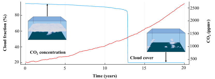
(a)

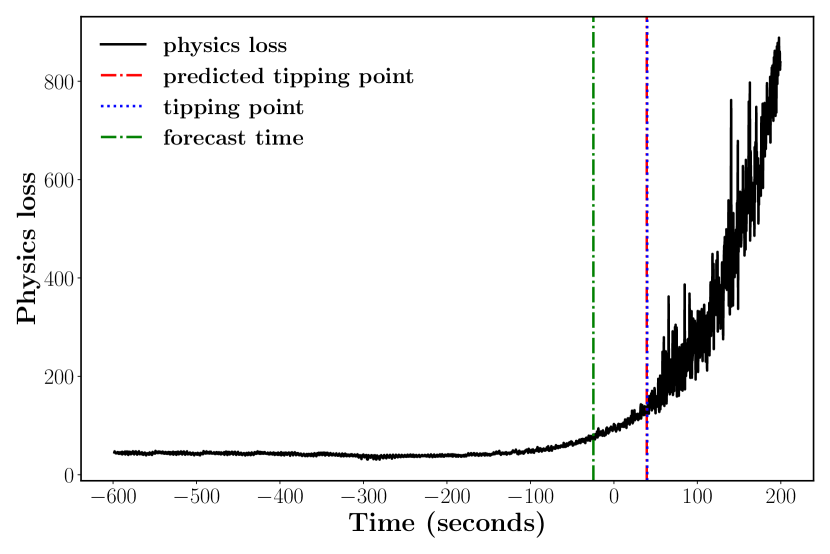
(b)

Figure 1: (a) Tipping point in cloud fraction as a function of $\text{CO}_{2}$ concentration, from bulk model of the atmospheric boundary layer developed in [5, 6]. 3d cloud cover renderings reproduced from [2]. (b) RNO accurately forecasts tipping point $64$ seconds ahead in non-stationary Lorenz-63 system. “Predicted tipping point” is the time at which our framework predicts a tipping point will occur, and “forecast time” is the time when our framework makes this prediction.

Method	Generality	Function space	Partial physics	Speed	Pre-tip data
Solver	✔	✔	✘	✘	N/A
EWS [7]	✘	✘	N/A	✔	✔
Bury et al. [8]	✘	✘	N/A	✔	✘
Patel and Ott [4]	✔	✘	N/A	✔	✘
Ours	✔	✔	✔	✔	✔

Table 1: Comparison of methods. “Generality” denotes applicability to arbitrary types of tipping points. “Pre-tip data” denotes the whether the method can forecast tipping points using only data from the pre-tipping regime.

Recent research introduced neural operators [9] for learning operators to remedy these shortcomings. Neural operators receive functions at any discretization as inputs, possess multiple layers of non-linear integral operators, and output functions that can be evaluated at any point. Neural operators are universal approximators of operators and can approximate continuous non-linear operators in PDEs [9]. These properties make neural operators discretization-invariant and suitable for learning in function spaces. Fourier neural operators (FNO) are architectures that use Fourier representations to integrate, providing an efficient implementation for many real-world applications. These methods, in particular Markov neural operators (MNO), have shown significant progress in learning Markov kernels of stationary dynamics systems [10]. However, non-stationary dynamical systems have potentially long memories, making earlier MNO developments not directly applicable to the setting of this paper.

In this work, we introduce recurrent neural operators (RNOs), a recurrent architecture for neural operators that enables learning memory-equipped maps on function spaces (Figure 2). RNO receives a sequence of historical continuous (in time) function data and represents the memory in terms of a latent state function. This enables conditional predictions for future functions given the latent functional representations of the past. In contrast to RNNs and other fixed-discretization approaches, RNO is discretization invariant in both space and time. We show that RNOs are capable of learning the dynamics of non-stationary chaotic systems and outperform RNNs and the state-of-the-art MNO by orders of magnitude on the non-stationary Lorenz-63 system, the Kuramoto-Sivashinsky (KS) equation, and a simplified model of stratocumulus cloud cover evolution [5, 6].

Tipping point forecasting.

A commonly observed trait of non-stationarity is the existence of abrupt, drastic, and often irreversible changes in system dynamics, known as tipping points [11]. Tipping points are conceptual reference points in non-stationary systems where the evolution undergoes a sudden change in quantities of importance. For instance, in the climate system, several tipping point phenomena have been identified [12, 13, 14], such as the collapse of the oceanic thermohaline circulation [15, 16, 17], ice sheet instability [18, 19, 20, 21], permafrost loss [22, 23], and low cloud cover breakup [2]. As shown in Figure 1(a), an increase in $\text{CO}_{2}$ in an idealized model is linked to a delayed drastic drop in cloud cover [2, 5, 6].

The identification and analysis of these climate tipping points typically relies on running numerical solvers for a very long time, which makes these methods extremely costly [2, 16]. Therefore, solvers are often run at low resolution or over subsets of the full domain, which can result in loss of accuracy or generality [2].

Recently, machine learning methods have been deployed for predicting the tipping points of non-stationary system [8, 4, 24, 25, 26, 27, 28, 29]. However, the prior works either focus on detecting domain shift instead of forecasting tipping points far ahead in time, and those that do forecast tipping points lack a systematic approach to learn non-stationary systems at arbitrary resolutions and forecast tipping points in function space.

In this work, we propose training an RNO model to predict future states on the complex dynamics of non-stationary chaotic systems using only data of pre-tipping point events. The set-up is motivated by climate modeling, where tipping points are not present in forty years of historical data [30]. To forecast the time of a tipping point, we build our approach based on the common observation that, at a tipping point, the prediction accuracy of machine learning models degrades due to distribution shifts [4, 24]. Since in our setting we do not have access to post-tipping data, we instead propose to forecast tipping points whenever the model prediction of the future exhibits extensive violations of domain-specific physical constraints. We use these physical constraints (e.g., conservation laws or governing PDEs) to verify the correctness of our model’s system forecasts at a given future time. Our method assumes that a given RNO model is well-trained on pre-tipping dynamics. Crucially, since the model is trained only on pre-tipping dynamics, even a perfect model on the pre-tipping regime would degrade in prediction accuracy beyond the tipping point, as observed empirically. We show that this approach predicts tipping points very far in advance.

To quantify the prediction accuracy, we propose a new conformal prediction method based on cumulative distribution functions (CDFs) [31]. We estimate the CDF of physics error, which quantifies the violation of physics constraints by the model’s forecasts and plays the role of a non-conformity score. We employ the fact that using finitely-many samples, a CDF of any distribution can be estimated accurately everywhere under the Kolmogorov–Smirnov distance, a property that is not true for other functions like quantiles [32, 33]. Using the empirical CDF of the physics error, we quantify the distribution of the non-conformity score. This uncertainty quantification is directly connected to the false positive rate of our prediction approach.

We consider the non-stationary and chaotic Lorenz-63 and Kuramoto–Sivashinsky (KS) systems, as well as a real-world system describing tipping points in stratocumulus cloud cover [5, 6]. We show that RNO consistently outperforms the state-of-the-art adapted baseline MNO in forecasting tipping points in these systems, particularly for the KS equation. We show that RNO better fits the underlying physical equations of the systems. Furthermore, we demonstrate under our proposed approach, RNO is able to accurately forecast tipping points when run for up to $200$ time intervals (Figure 1(b)).

In summary, we propose the first tipping point forecasting framework that scales to arbitrary tipping points and arbitrary spatiotemporal systems on function spaces. In particular, we

1. Introduce RNO, a data-driven operator learning approach to learn the dynamics of arbitrary non-stationary systems.

2. Construct a tipping point forecasting framework that relies only on (1) a data-driven model of pre-tipping dynamics and (2) a physical constraint of the system.

3. Propose a novel conformal prediction method to quantify deviations in model physics error in a statistically rigorous manner.

4. Achieve accurate tipping point forecasting far in advance for PDE and ODE systems.

5. Demonstrate high accuracy in tipping point forecasting using approximate and partial physical constraints, generalizing our method to settings when full physics laws are unknown.

2 Related Work

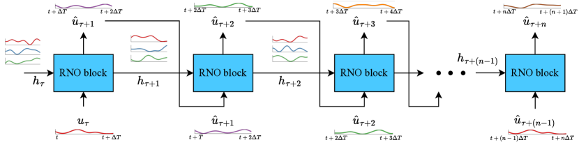
Figure 2: Illustration of RNO auto-regressive forecasting.

Tipping points exhibit complex behavior, making their study a challenging task in the high-dimensional multi-modal setting [1]. In recent years, tipping points and their root causes have been categorized for simple systems (such as low-dimensional ODEs), based on stochasticity, rate change, and bifurcations [11, 34, 35]. Tipping points can be caused by changes in the condition and sourcing in differential equations, or sometimes, the root cause is the rate at which these conditions change [11]. However, in the case of general scientific computing problems on natural phenomena, theoretical studies of tipping points are very challenging, and prior works have primarily focused on their empirical evaluation via numerical simulation.

Tipping points are abundant in scientific computing of climate evolution and control modeling [12, 13, 14]. Previous work has highlighted the importance of predicting tipping points in the Earth system with the goal of giving early warning ahead of large changes in the climate [36, 37]. Approaches have varied depending on the type of tipping behavior considered [38]. For instance, it has been shown that changes in atmospheric CO₂ levels can cause rapid changes in low cloud cover on the Earth [2, 6]. And furthermore, after bringing CO₂ levels below the tipping threshold, these changes may not be readily undone (the system exhibits hysteresis).

Traditional early warning signals (EWS) of tipping points such as increased autocorrelation before tipping events have been studied extensively for many simple systems [39, 40]. However, tipping points in the large spatiotemporal systems that motivate this work have not yet been sufficiently studied empirically and theoretically for these indicators to become evident. Furthermore, for many spatiotemporal systems, thorough empirical evaluation is difficult due to the computational cost of simulations. Thus, data-driven approaches for learning system dynamics and forecasting tipping points is critical for most challenging real-world problems. In Appendix F.2, we demonstrate that EWS are not reliable at predicting tipping points in the systems we study. Recently, machine learning methods have been deployed for learning in non-stationary dynamical systems and to predict their tipping points [8, 4, 24, 25, 26, 27, 28, 29]. However, many works require post-tipping data [4, 8], full governing equations [26], or are not generalizable to arbitrary types of tipping points [8, 28]. In contrast, our method is scalable, does not need full governing equations, and is not trained on post-tipping data. See Table 1 and Appendix F.1 for a detailed comparison with prior work.

RNNs are often used to learn in finite-dimensional dynamical systems with memory or in time-series with discrete-time dynamics [3, 41]. They consist of blocks of neural networks that carry memory as a finite-dimensional latent state and enable conditional predictions on learned latent historical representations. But since neural networks are maps between finite-dimensional spaces, RNNs are unfit for many scientific computing problems, which often involve functions (i.e., infinite-dimensional objects) and their time-evolution. Neural ODE versions of RNNs have similar issues, can only model specific time derivatives, and require expensive solvers for temporal simulation [42, 43, 44].

Neural operators are deep learning models that generalize neural networks to maps between function spaces [45, 46, 47], and they are universal approximators of general operators [9]. The inputs to neural operators are functions, and the output function can be evaluated at any point in the function domain. These models are thus known to be discretization invariant and can take the input function at any resolution. In this paper, we develop the recurrent neural operator (RNO). RNO receives a sequence of historical function data and represents the memory in terms of a latent state function, enabling conditional predictions given learned latent functional representations of the past.

3 Preliminaries

A PDE is differential law on function spaces. For an input function $a$ from a function space $\mathcal{A}$, we denote $\mathcal{D}_{\mathcal{A}}$ as the domain and $\mathbb{R}^{d_{\mathcal{A}}}$ as the function co-domain with dimension $d_{\mathcal{A}}$. For any point in the domain $x\in\mathcal{D}_{\mathcal{A}}$, the function $a$ maps this point to a $d_{\mathcal{A}}$-dimensional vector, i.e, $a(x)\in\mathbb{R}^{d_{\mathcal{A}}}$. Correspondingly, let $\mathcal{U}$ denote the solution or output function space, defined on domain $\mathcal{D}_{\mathcal{U}}$ with co-domain $\mathbb{R}^{d_{\mathcal{U}}}$, i.e., for any function $u\in\mathcal{U}$ and any $x\in\mathcal{D}_{\mathcal{U}}$, we have $u(x)\in\mathbb{R}^{d_{\mathcal{U}}}$. For a given $a$, we define a PDE in generic form as,

$$\begin{split}\mathcal{L}(u,a)(x)&=0,\qquad\text{in }\mathcal{D}_{\mathcal{U}},\\ \mathcal{L}^{\prime}(u,a)(x)&=0,\qquad\text{in }\partial\mathcal{D}_{\mathcal{U}},\end{split}$$ (1)

where $\mathcal{L}(u,a)$ is the governing law in the domain $\mathcal{D}_{\mathcal{U}}$, and $\mathcal{L}^{\prime}(u,a)(x)$ is the constraint on the domain boundary $\partial\mathcal{D}_{\mathcal{U}}$. A function $u$ is a solution to the above PDE at input $a$ if the function $u$ satisfies both of the PDE constraints (Eq. 1), comprising an input-solution pair $(a,u)$. We are concerned with learning maps from input function spaces $\mathcal{A}$ to output function spaces $\mathcal{U}$ in operator learning. For a given PDE, let $\mathcal{G}^{\star}$ denote the operator that maps the input functions in $\mathcal{A}$ to their corresponding solution functions in $\mathcal{U}$, a map that employs a neural operator to learn.

A neural operator $\mathcal{G}$ is a deep learning architecture consisting of multiple layers of point-wise and integral operators [9] to learn a map from input function $a$ to output function $u$. The first layer of the architecture is a pointwise lifting operator $\mathcal{P}_{0}$ such that for a given function $a$, the output of this layer $\nu_{0}=\mathcal{P}_{0}a$ is computed so that for any $x\in\mathcal{D}_{\mathcal{A}}$, $\nu_{0}(x)=P_{0}(a(x))\in\mathbb{R}^{d_{0}}$ where $P_{0}$ is a learnable neural network. This step is followed by $L$ layers of nonlinear integral operators. For any layer $l$ we have,

$$\nu_{l}=\mathcal{P}_{l}(\sigma(\mathcal{K}_{l}\nu_{l-1})+\mathcal{W}_{l}\nu_{l-1}s_{l}),$$ (2)

where $\nu_{l}:D_{l}\rightarrow\mathbb{R}^{d}_{l}$, $\sigma$ is some pointwise nonlinearity, and $\mathcal{K}_{l}$ is an integral operator such that for any $x\in\mathcal{D}_{l}$, we have,

$$\mathcal{K}_{l}\nu_{l-1}(x)=\int_{\mathcal{D}_{l-1}}\kappa_{l}(x,y)\nu_{l-1}d\mu_{l}(y)+\mathcal{W}_{l}^{\prime}\nu_{l-1}(s_{l}(x)).$$ (3)

Here $\kappa_{l}$ is a learnable kernel function, $\mathcal{W}_{l}^{\prime}$ is a pointwise operator parameterized by a neural network $W_{l}^{\prime}$, and $s_{l}$ is a deformation map from $\mathcal{D}_{l}$ to $\mathcal{D}_{l-1}$. Similarly, $\mathcal{W}_{l}$ is a pointwise operator parameterized by $W_{l}$ neural network, and $\mathcal{P}_{l}$ is a pointwise operator parameterized by a neural network $P_{l}$. $\mu_{l}$ represents the measure on each space and finally, we set $\mathcal{D}_{L}=\mathcal{D}_{\mathcal{U}}$. The last layer is a pointwise projection operator $\mathcal{Q}$ parameterized by a neural network $Q$. In particular, we use Fourier representations to compute the integration Eq. 3 in its convolution form,

$$\mathcal{K}_{l}\nu_{l-1}(x)=\mathcal{F}^{-1}\mathcal{F}\kappa_{l}\cdot\mathcal{F}\nu_{l-1}+\mathcal{W}_{l}^{\prime}\nu_{l-1}(s_{l}(x)),$$ (4)

where $\mathcal{F}$ denotes the Fourier transform, and project its inputs to $k_{l}$ Fourier bases, for some hyperparameter $k_{l}$. Let $R_{l}$ denote the $k_{l}$ Fourier coefficients of $\kappa_{l}$, i.e., $R_{l}=\mathcal{F}\kappa_{l}$. Following [46], we directly learn $R_{l}$ instead of $\kappa_{l}$ to learn the integral operator. We utilize these building blocks to construct the RNO architecture in the next section.

4 Recurrent neural operator (RNO)

We now describe and formulate RNO, a generalization of RNNs to function spaces. For a given PDE describing the evolution of a function $u(x,t)$ of time and space, consider a partition of the time domain $t$ into equally-spaced intervals of length $\Delta T$ and indexed by $\tau\in\mathbb{N}$. A step $\tau$ is associated with the interval $[(\tau-1)\cdot\Delta T,\tau\cdot\Delta T]$, where the input function restricted to this interval is defined for $t\in[t,t+\tau\cdot\Delta T]$ as $u_{\tau}(x,t):=u(x,t)$.

Our proposed architecture of the RNO parallels that of the gated recurrent unit (GRU) [48], where the GRU cell at step $\tau$ receives a hidden state vector $h_{\tau}$ and an input vector $x_{\tau}$, and predicts the next output vector $x_{\tau+1}$ and next hidden state vector $h_{\tau+1}$, which is also passed to the GRU cell at step $\tau+1$. The key difference between the RNO and the GRU is that at step $\tau$, an RNO cell receives as input a hidden function $h_{\tau}(x,t)$ and an input function $u_{\tau}(x,t)$. As such, we replace the linear maps in the GRU architecture with Fourier layers, Eq. 4). Given $u_{\tau}$ and $h_{\tau}$, we define the reset gate such that for any $t\in[t,t+\tau\cdot\Delta T]$,

$$r_{\tau}(x,t)=\sigma\Big{(}(\mathcal{K}_{r}u_{\tau})(x,t)+(\mathcal{K}^{\prime}_{r}h_{\tau})(x,t)+b_{r}(x,t)\Big{)},$$ (5)

where $\mathcal{K}_{r},\mathcal{K}^{\prime}_{r}$ are Fourier layers, $b_{r}(x,t)$ is a learned bias function, and $\sigma$ is the sigmoid function applied pointwise. We define the update gate as,

$$z_{\tau}(x,t)=\sigma\Big{(}(\mathcal{K}_{z}u_{\tau})(x,t)+(\mathcal{K}^{\prime}_{z}h_{\tau})(x,t)+b_{z}(x,t)\Big{)}.$$ (6)

We define the candidate hidden function as,

$$\widehat{h}_{\tau+1}(x,t)=\phi\Big{(}(\mathcal{K}_{h}u_{\tau})(x,t)+(\mathcal{K}^{\prime}_{h}(r_{\tau}\cdot h_{\tau}))(x,t)+b_{h}(x,t)\Big{)},$$ (7)

where $\phi$ denotes a point-wise scaled exponential linear unit (SELU) activation and the function multiplication $(\cdot)$ is taken to be pointwise. Finally, we define the hidden state function $h_{\tau+1}(x,t)$ as

$$h_{\tau+1}(x,t)=\Big{(}(1-z_{\tau})\cdot h_{\tau}\Big{)}(x,t)+\Big{(}z_{\tau}\cdot\widehat{h}_{\tau+1}\Big{)}(x,t).$$ (8)

We take $h_{0}(x,t)$ to be a learned prior function on the initial hidden state. Let $\text{{\small{RNO}}}(v,h_{\tau})$ denote an RNO cell. Given the input function $u_{\tau}$, an RNO block takes the following form:

$$\tilde{u}_{\tau}(x,t) =\mathcal{P}_{0}(u_{\tau})(x,t)=P_{0}(u_{\tau}(x,t)),$$ (9)

$$v^{(i+1)}_{\tau}(x,t) =\text{{\small{RNO}}}^{(i+1)}\left(v^{(i)}_{\tau},h^{(i+1)}_{\tau}\right)(x,t),$$ (10)

$$\widehat{u}_{\tau}(x,t) =\mathcal{Q}(v^{(L)}_{\tau})(x,t)=Q(v^{(L)}_{\tau}(x,t)),$$ (11)

where $\mathcal{P}_{0}$ and $Q$ are pointwise lifting and projection operators, respectively parameterized by neural networks $P_{0}$ and $Q$. $v^{(0)}_{\tau}(x,t):=\tilde{u}_{\tau}(x,t)$, the result of the lifting operation, and $L$ is the number of RNO layers. An RNO is then a RNO block evolving in time with $h^{(i)}_{\tau+1}:=v^{(i)}_{\tau}$ for each RNO cell $i\geq 1$, Figure 2.

We divide the inference stage of RNO into two phases:

1. Warm-up phase: In the warm-up phase, we have access to the ground-truth trajectory between steps $\tau=0$ and $\tau=N_{\tau}-1$, corresponding to the ground-truth solution $u(t)$ between times $t\in[0,N_{\tau}\Delta T]$. During this phase, the RNO blocks receive as input $u_{\tau}$, and the predicted $\widehat{u}_{\tau+1}$ is discarded.

2. Prediction phase: In the prediction phase, we assume we no longer have access to the ground-truth trajectory beyond time $\tau=N_{\tau}-1$, so the model predictions $\widehat{u}_{\tau+j}$ are taken as input to the RNO block at time $\tau+j+1$, and the model is thus composed with itself (with access to its hidden state $h_{\tau}$), with its outputs fed back on itself as inputs.

The prediction phase is similar to Markov neural operator (MNO) [10], with the exception that RNO now has access to a continually-updating hidden representation $h_{\tau}(x,t)$, which encodes the history of the non-stationary system, making RNO a generalization of MNO to systems with memory.

5 Tipping-point Forecasting

Forecasting tipping points requires rigorous uncertainty quantification, and any prediction must be accompanied by the event’s potential probabilities. Conformal prediction is a field of study that accompanies predictions with certainty levels in terms of a conformity score [31]. Most prior work on traditional conformal prediction quantifies the probability distribution of the conformity score at certain levels. Another approach is to utilize quantile regression to quantify the distribution of conformity scores  [49]. Both of these approaches have shortcomings in tipping point prediction. The former approach utilizes exchangeability and requires new and fresh draws of samples to quantify the distribution of conformity scores, imposing a union bound over a long period of time. Quantile regression suffers from two downsides: (1) quantiles are not generally estimable, and (2) a union bound over an infinite set is required to quantify the conformity score distribution [50]. These limitations are addressed below by introducing CDF estimation methods.

Our tipping point forecasting utilizes training on the pre-tipping dynamics of the system. We train RNO on data sets of time-evolving functions that do not contain any tipping points. We make this choice to resemble real-world settings such as climate where recorded historical data does not contain tipping points. At any time $t$, we use RNO to predict the long evolution of the dynamics for an interval of $[t,t+T]$, i.e., $\widehat{u}(x,[t,t+T])$ where $T$ is a multiple of $\Delta T$. At the forecast time $t$, we do have access to the future $u(x,[t,t+T])$. If we did, we could use the deviation of $\widehat{u}(x,[t,t+T])$ from $u(x,[t,t+T])$ as a hindsight indicator for the tipping point as observed in prior works [4, 24].

Instead, we propose to use the physical constraints $\mathcal{L}(u)=0$ of the underlying system (such as the PDE that governs the dynamics) to evaluate the deviation of $\widehat{u}(x,[t,t+T])$ from physics laws, and we use this signal as an indicator of tipping points. For a predicted function $\widehat{u}(x,[t,t+T])$, we define the conformity score as $\|\mathcal{L}(\widehat{u})-0\|$, and we refer to it by the physics loss $\ell_{P}(\widehat{u})$. Note that if $\widehat{u}(x,[t,t+T])=u(x,[t,t+T])$ (the true future function), then $\mathcal{L}(\widehat{u})=0$, and thus our proposed indicator aligns with the hindsight indicator mentioned above. At any time $t$, we compute $\ell_{P}(\widehat{u})$, and if it takes values above a certain threshold, we forecast that a tipping point is anticipated. This method enables tipping point forecasting. However, since the trained model comes with training generalization error, this approach makes mistakes, confusing large errors on pre-tipping regimes and actual tipping incidence. This is of particular importance when the forecasting interval of interest $T$ is large. We propose the following novel conformal prediction to address uncertainty quantification in tipping point forecasting.

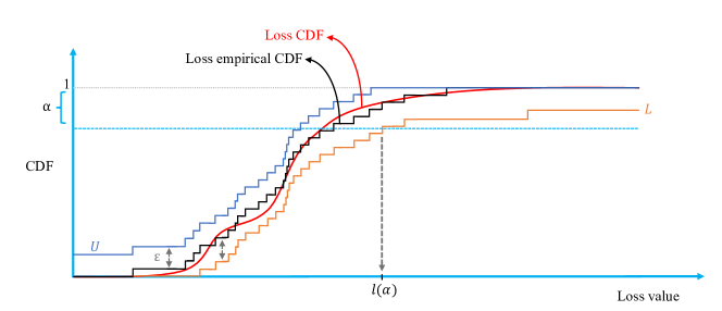
Figure 3: Diagram of the setup for the tipping point prediction method. $U$ and $L$ correspond to the upper and lower bounds given by the CDF concentration inequality, differing from the empirical CDF by $\varepsilon$. $\alpha$ is the significance level, and $l(\alpha)$ is the corresponding loss of $L$ at $\alpha$.

For a trained model and given a forecasting interval $T$, let $F$ denote the true CDF of the conformity score. The CDF captures the probabilities at which the model makes errors of a given magnitude on pre-tipping data. We use the CDF to develop our conformal prediction method, which allows for uncertainty quantification of tipping point forecasts. In particular, for any loss threshold at which we call a tipping point, we can denote $\alpha$ to be the probability of falsely forecasting a tipping point when the data was simply from the pre-tipping regime. We first compute the empirical CDF $\widehat{F}$ of the conformity score $\ell_{P}(u)$ using $n$ calibration samples. Formally, given $n$ samples, we construct $\{{\ell_{P}}^{(j)}\}_{j=1}^{n}$ and compute $\widehat{F}$ as follows. For any $p\in\mathbb{R}$,

$$\widehat{F}(p):=\frac{1}{n}\sum_{j}^{n}\mathbbm{1}(p\geq{\ell_{P}}^{(j)}).$$

We then use the concentration inequality of CDFs to compute its upper and lower bounds [32, 33]. Using the concentration inequality of CDFs, with probability at least $1-\delta$ we have,

$$\sup_{p\in\mathbb{R}}\left|\widehat{F}(p)-F(p)\right|\leq\varepsilon:=\sqrt{\frac{\log(2/\delta)}{2n}},$$

where the left-hand side is the Kolmogorov–Smirnov distance between the two CDFs. We define the CDF lower bound $L(p):=\max\{0,\widehat{F}(p)-\varepsilon\}$ and the CDF upper bound $U(p):=\min\{1,\widehat{F}(p)+\varepsilon\}$. Figure 3 depicts this procedure. Intuitively, $\alpha$ denotes the maximum probability of a mistake that one is willing to tolerate. In our approach, as shown in Figure 3, we first find $l(\alpha)$, the conformity level at which the CDF lower bound $L$ has probability $1-\alpha$. Using the level $l(\alpha)$, we call the presence of a tipping point whenever the conformity score of our prediction $\ell_{P}(\widehat{u})$ is above $l(\alpha)$.

Proposition.

For any given $\alpha\in[0,1]$, the decision rule of calling for a tipping point at level $l(\alpha)$ has a false positive rate of at most $\alpha$, and this statement holds with probability at least $1-\delta$.

The proof is based on the fact that for any $\alpha$, $F^{-1}(1-\alpha)\leq l(\alpha)$ and $F(l(\alpha))\geq 1-\alpha$. Therefore, when $\ell_{P}\geq l(\alpha)$, signaling a tipping point, we also have $\ell_{P}\geq F^{-1}(1-\alpha)$. Thus, the probability of the event $\ell_{P}\geq l(\alpha)$ is lower bounded by the probability of $\ell_{P}\geq F^{-1}(1-\alpha)$ which at most $\alpha$. This proposition simultaneously holds for all the time steps $\tau$ and all $\alpha$. This property enables assessing tipping predicting at various levels, a crucial feature for risk assessment and policy making.

6 Experimental Results

We present experimental results on learning dynamics and forecasting tipping points in non-stationary systems. We showcase the performance of RNO and the tipping point forecasting method on the finite-dimensional Lorenz-63 system, the (infinite-dimensional) KS PDE, and the example of tipping points in simplified cloud cover equations. Discussion on the technical details of RNO (e.g., memory usage, inference times, hyperparameter selection, etc.) can be found in Appendix G.

6.1 Non-stationary Lorenz-63 system

We consider tipping point forecasting in the non-stationary chaotic Lorenz-63 system [51], a simplified model for atmospheric dynamics. The non-stationary Lorenz-63 system is given by

$$\dot{u}_{x}=\sigma(u_{y}-u_{x}),\qquad\dot{u}_{y}=u_{x}(\rho(t)-u_{z})-u_{y},\qquad\dot{u}_{z}=u_{x}u_{y}-\beta u_{z},$$ (12)

where the state space is $u=(u_{x},u_{y},u_{z})$, and the parameters of the system are $\sigma,\rho(t),\beta$, where $\rho$ depends on time as in [4].

We find that RNO substantially outperforms MNO and RNN in learning the evolution of the non-stationary system. Furthermore, we use the Lorenz-63 system as a case study to justify our tipping point forecasting framework. Figure 1(b) shows that RNO is capable of accurately forecasting the tipping point $64$ seconds ($T=200\cdot\Delta T$) ahead, even though the size of each input/output interval is $\Delta T=0.32$ seconds. The full experimental setup and results can be found in Appendix A.

We also demonstrate that our method is capable of forecasting tipping points far in advance using only approximate knowledge of the underlying system. In particular, we perturb the parameters $\sigma,\rho,\beta$ by some fixed quantity $\eta$ and show that the error in the tipping point forecast for the Lorenz-63 system is still less than $1$ second, even when predicting $64$ seconds in advance. Results can be found in Appendix A.

6.2 Non-stationary Kuramoto–Sivashinsky (KS) equation

We demonstrate the effectiveness of RNO and our tipping point forecasting method in PDE systems by considering the 1-d non-stationary KS equation, which takes the form

$$\frac{\partial u}{\partial t}+u\frac{\partial u}{\partial x}+\frac{\partial^{2}u}{\partial x^{2}}+\kappa(t)\frac{\partial^{4}u}{\partial x^{4}}=0$$ (13)

where $\kappa(t)$ is some time-dependent parameter of the system, $u(x,t)$ is a function of space $x\in[0,2\pi]$ and time $t\in(0,\infty)$, and the initial condition is $u(\cdot,0)=u_{0}$. Following [4], we parameterize $\kappa(t)=\kappa_{0}+\kappa_{1}\exp(t/\gamma)$, where $\kappa_{0}=0.0753$, $\kappa=0.0034$, and $\gamma=75.3$. This system exhibits a tipping point near $\kappa^{*}=0.08$ from periodic dynamics to chaotic dynamics. The tipping point can be classified as an instance of bifurcation-induced tipping [11] at a saddle-node bifurcation [4].

Model	1-step	2-step	4-step	8-step	12-step	16-step	20-step
RNO	$\mathbf{0.0030}$	$\mathbf{0.0027}$	$\mathbf{0.0031}$	$\mathbf{0.0419}$	$\mathbf{0.1410}$	$\mathbf{0.2919}$	$\mathbf{0.4008}$
MNO	$0.0050$	$0.0073$	$0.0150$	$0.2901$	$1.0751$	$1.2626$	$1.3772$
RNN	$0.0525$	$0.0481$	$0.1443$	$0.5488$	$0.9031$	$1.0031$	$1.1561$

Table 2: Relative $L^{2}$ errors on non-stationary KS equation for different $n$-step prediction settings. RNO outperforms both MNO and the baseline RNN on every forecasting intervals.

6.2.1 Learning non-stationary dynamics

We compare RNO against Markov neural operators (MNO) [10] and RNNs in forecasting non-stationary dynamics. There are two key properties that any learned model must exhibit: (1) low step-wise error and (2) error stability in long-time predictions (i.e., when the model is composed with itself many times). Low step-wise error is a necessary prerequisite to adequately learning the dynamics of any system. However, for many downstream tasks of significant scientific importance, it is also crucial that our model’s error remain low when forecasting far into the future. This ensures the accuracy of tipping point prediction is credible in complex real-world settings. Hereafter, we define “$n$-step prediction” to be a model’s forecasting prediction looking ahead $\tau=n$ steps.

In our experiments, we employ a multi-step training regimen for all models, where the total loss is a combination of the loss on the model’s $n$-step prediction for $n\in\{1,2,\dots,M\}$. That is, our data loss function is given by

$$\ell_{D}(u,\widehat{u})=\sum_{n=1}^{M}\lambda_{n}\|u_{n}-\widehat{u}_{n}\|_{2},$$ (14)

where $\|\cdot\|_{2}$ is the $L^{2}$ norm and $\lambda_{n}$ is some scaling hyperparameter.

Table 2 compares the relative $L^{2}$ errors of RNO, MNO, and RNN on forecasting the non-stationary KS equation. We observe that RNO outperforms MNO and RNN on every forecasting interval. Further, we can observe the disadvantages of RNN and other finite-dimensional, fixed-resolution models on learning in PDE (i.e., infinite-dimensional) settings. The RNN’s error is orders of magnitude larger than that of RNO or MNO for small forecasting windows. At large forecasting windows (i.e., 12-step and above), the lack of explicit history in MNO becomes a severe disadvantage. In contrast, RNO maintains much lower error at large forecasting intervals than the other two models. Both the MNO and RNO shown in Table 2 were trained with $M=5$ steps of fine-tuning (Eq. 14). Observe that MNO and RNN have difficulty generalizing to forecasting intervals larger than $M$, whereas RNO is capable of maintaining stable error even at longer forecasting intervals.

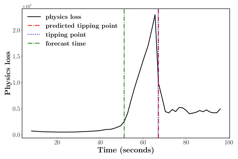
(a) RNO

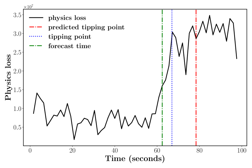
(b) MNO

Figure 4: (a) RNO accurately forecasts tipping point $16$ seconds ahead in non-stationary KS system. Right after the abrupt change at the tipping point, the physics loss decays for post-tipping. (b) MNO fails to accurately forecasting tipping point in KS system. A false-positive rate of $\alpha=0.07$ is used.

6.2.2 Tipping point forecasting

In this section, we present empirical results in tipping point prediction for the non-stationary KS equation. As described in Section 5, our conformal prediction approach for tipping point prediction relies on a model trained in pre-tipping dynamics. We then monitor variations in the physics constraint loss of model forecasts to predict tipping points in the future. Recall that the physics constraint loss is only a function of the model predictions $\widehat{u}$ and the time $t$. We define the KS physics loss to be

$$\ell_{P}(\widehat{u},t)=\left\|\frac{\partial\widehat{u}}{\partial t}+\widehat{u}\frac{\partial\widehat{u}}{\partial x}+\frac{\partial^{2}\widehat{u}}{\partial x^{2}}+\kappa(t)\frac{\partial^{4}\widehat{u}}{\partial x^{4}}\right\|_{2}.$$ (15)

In practice, $\ell_{P}$ is computed over an entire calibration set, which is unseen during training, and these samples are used to construct an empirical CDF of the physics loss.

In our experiments, we consider the setting of forecasting tipping points far ahead in time, at several orders of magnitude longer time scales than the model is trained on. For the KS equation, we set $\Delta T=1.6$ seconds. Figures 4(a) and 4(b) compare the accuracy of RNO and MNO in forecasting the KS tipping point $T=16$ seconds ahead. At short forecasting intervals (e.g., $T=\Delta T$ or $T=2\cdot\Delta T$), RNO and MNO both accurately capture the tipping point, but at long time-scales only RNO retains good performance.

6.3 Cloud cover equations: tipping points from partial physics

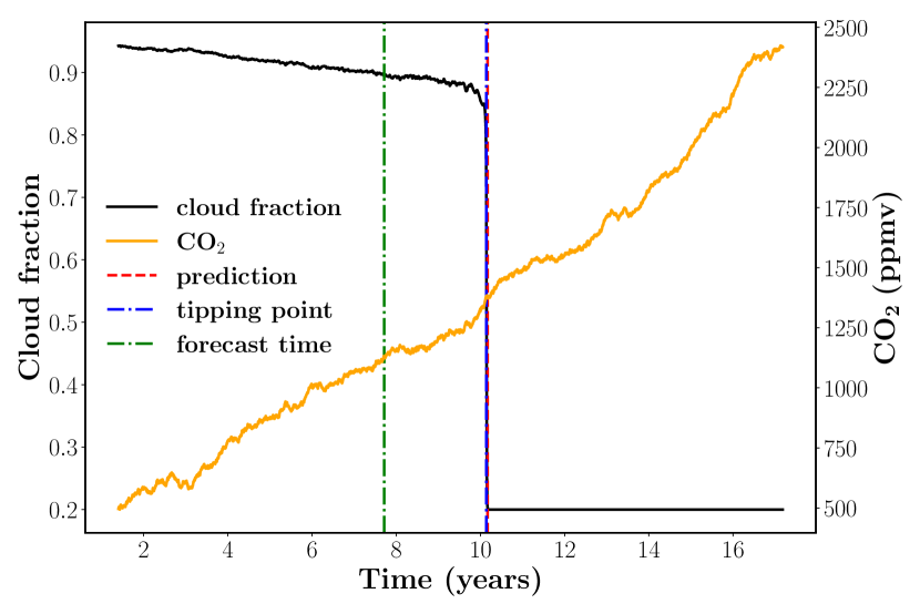
(a) Tipping point forecast w.r.t. cloud fraction

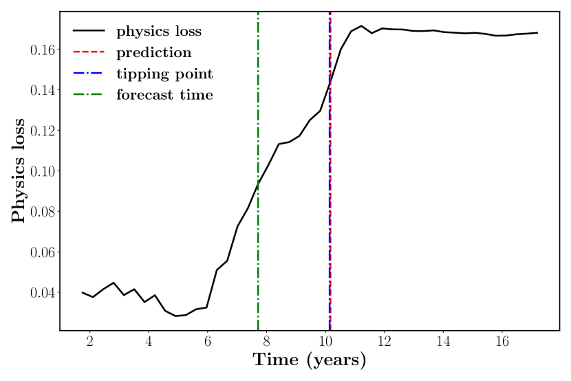
(b) Tipping point forecast w.r.t. partial physics loss

Figure 5: For the cloud cover model, using only a mass conservation constraint (as opposed to the full system), RNO is still capable of identifying the true tipping point of the system with an error of $0.03$ years, predicting $T=2.45$ years ahead, at $\alpha=0.07$.

We now consider a case study of tipping point forecasting in the Earth’s climate. We also demonstrate that our method is still accurate under partial physics, e.g., conservation laws (not full PDEs).We use the model developed in [5, 6] as an idealization of the physical climate system; this model exhibits a tipping point. The model represents a stratocumulus-topped atmospheric boundary layer, which experiences rapid loss of cloud cover under high CO₂ concentrations and shows hysteresis behavior, where the original state is not immediately recovered when CO₂ concentrations are lowered. This model was developed, in part, to help explain the results found from the high-resolution simulations in [2, 52]. More details on the model can be found in Appendix B, and details on numerical experiments can be found in Appendix E.4.

Analogously to the KS equation setting (Section 6.2), we train an RNO to forecast the non-stationary evolution of the system with a data loss given by Eq. 14, which incorporates the $L^{2}$ loss across longer time horizons. We compute the empirical CDF of the physics loss for the cloud cover system (analogous to Eq. 15 in the KS setting) as a function of model predictions and CO₂. However, in this case, the physics loss is normalized component-wise by the state of the system at a given time, since the magnitudes of each component in this model differ by several orders of magnitude.

For tipping point forecasting, we base the physics loss solely on mass conservation (Eq. 18a), instead of the full ODE. In our experiments, we set the tipping point forecasting horizon to be $T=7\cdot\Delta T=2.45$ years (with forecasting intervals of $\Delta T=0.36$, or 128 days). We found that the choice of $\Delta T$ (on time-scales on the order of $O(100)$ days) does not significantly impact the RNO’s ability to learn the dynamics. $T$ is chosen to be an order of magnitude larger than $\Delta T$, to demonstrate that our framework is capable of forecasting tipping points at time-scales much longer than $\Delta T$. The results on a given test trajectory can be seen in Figure 5. Despite the abruptness of the tipping point and the highly-nonlinear dynamics of the system around the tipping point, we demonstrate that our forecasting framework is successfully able to identify the true tipping point in this system using a physics loss derived from a partial picture of the full physics.

7 Conclusion

In this paper, we introduce recurrent neural operator (RNO), an extension of recurrent neural networks to function spaces, and an extension of neural operators [9] to systems with memory. We also propose a model-agnostic conformal prediction method with considerable statistical guarantees for forecasting tipping points in non-stationary systems by measuring deviations in a model’s violations of underlying physical constraints or equations. In our experiments, we demonstrate RNO’s ability to learn non-stationary dynamical systems, particularly its stability in error even when auto-regressively applied for long time scales. We also demonstrate the effectiveness of our tipping point forecasting method on infinite-dimensional PDE systems, and we demonstrate that our proposed methodology maintains good performance even when using partial or approximate physics laws.

Appendix A Lorenz-63 experimental results

The Lorenz-63 system is defined in Eq. 12. In this paper, we follow the setting of [4] where $\sigma=10$, $\beta=8/3$, and $\rho$ depends on time via the parameterization $\rho(t)=\rho_{0}+\rho_{1}\exp\left(t/{\gamma}\right)$, where $\rho_{0}=154$, $\rho_{1}=8$, and $\gamma=100$.

A tipping point for this system occurs at approximately $\rho^{*}=166$ [53], which correspond approximately to time $t^{*}=40$ under the parameterization above. This tipping point is induced by an intermittency route to chaos [53] as the dynamics transition from periodic $t<t^{*}$ to chaotic $t>t^{*}$. The tipping point can be classified as an instance of bifurcation-induced tipping [11] at a saddle-node bifurcation [4]. Details on data generation and experimental setup can be found in Appendix E.

A.1 Learning non-stationary dynamics

Numerical results from our experiments are shown in Table 3. We observe that RNO outperforms MNO in relative $L^{2}$ error by at least an order of magnitude for every $n$-step prediction setting up to and including 32-step prediction. We observe that even when composed with itself 32 times, RNO is capable of maintaining relative $L^{2}$ error under $0.05$. Further, we find that despite training MNO with a multi-step procedure up to $M=12$ steps, this still does not prevent MNO error from steadily increasing as the number of steps to compose increases. While RNN is somewhat stable in its error when composed multiple times, RNO vastly outperforms it in $L^{2}$ error. We attribute the performance of RNO to its status as an architectural generalization of MNO to systems with memory. Further, RNO’s discretization invariance and adaptability to function spaces makes it an improvement over fixed-resolution RNNs.

A.2 Tipping point prediction: fully-known physics

Analogously to the KS setting (Eq. 15), we define the physics constraint loss to be

$$\ell_{P}(\widehat{u},t)=\left\|\dot{\widehat{u}}(t)-\widehat{\dot{u}}(t)\right\|_{2},$$ (16)

where $\dot{\widehat{u}}$ is the time-derivative of the model’s forecasted trajectory at time $t$ and $\widehat{\dot{u}(t)}$ is the time derivative defined by the Lorenz-63 system (eq. 12) using the model’s predicted state $\widehat{u}(t)$ at time $t$. That is,

$$\widehat{\dot{u}_{x}}=\sigma(\widehat{u}_{y}-\widehat{u}_{x}),\qquad\widehat{\dot{u}_{y}}=\widehat{u}_{x}(\rho(t)-\widehat{u}_{z})-\widehat{u}_{y},\qquad\widehat{\dot{u}_{z}}=\widehat{u}_{x}\widehat{u}_{y}-\beta\widehat{u}_{z}.$$ (17)

Thus, $\ell_{P}$ is minimized when the time derivative of the model’s predictions is equal to the expected derivative that all solutions to the Lorenz-63 system must satisfy (Eq. 12).

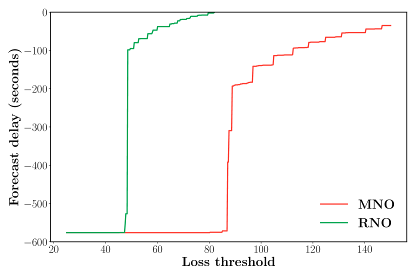
(a)

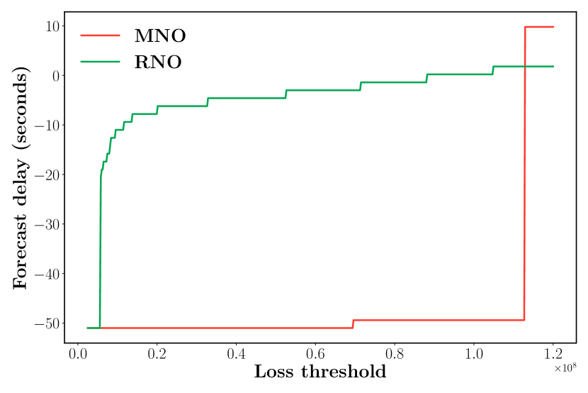
(b)

Figure 14: (a) Physics loss threshold comparison between RNO and MNO for non-stationary Lorenz-63 system predicting 64 seconds ahead. (b) Physics loss threshold comparison between proposed RNO and the state-of-the-art baseline MNO in non-stationary Kuramoto–Sivashinsky system for forecasting the tipping point $16$ seconds ahead. Negative numbers correspond to tipping points predicted early. RNO consistently outperforms MNO in tipping point forecasting for a given physics loss threshold, demonstrating that RNO learns the physics of the underlying system better that MNO.

In our experiments, we set $\Delta T=0.32$ seconds. Here we study the difficult task of forecasting the tipping point $64$ seconds ahead, corresponding to two hundred times the time scale of the model. For a fixed $\delta=10^{-3}$, Figure 14(a) shows the effect of varying the critical loss threshold $l(\alpha)$ for a given $\alpha$ on RNO and MNO tipping point predictions.

(a)

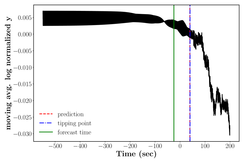
(b)

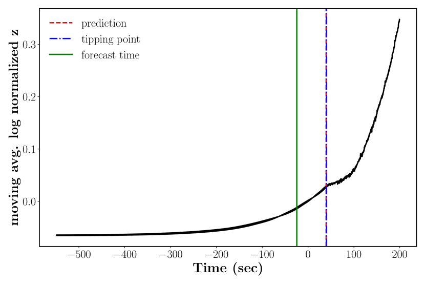
(c)

Figure 6: Log normalized components of the non-stationary Lorenz-63 system plotted with a 50-second moving average. The predicted tipping point aligns nearly exactly with the true periodic-chaotic tipping point of the system, which can be seen as a qualitative change in dynamics of the system components. A false-positive rate of $\alpha=\varepsilon\approx 0.03$ is used, where $\varepsilon$ is discussed in Section 5.

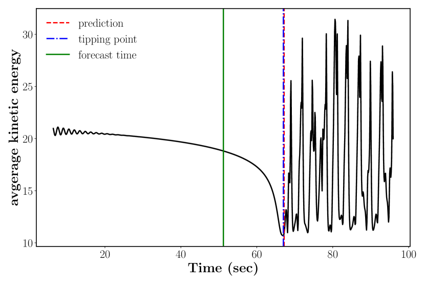
Figure 7: Kinetic energy of the non-stationary KS system. The predicted tipping point aligns nearly exactly with the true tipping point of the system, which can be seen as a qualitative change in the kinetic energy of the system. The false-positive rate is $\alpha=0.07$.

Model	1-step	2-step	4-step	8-step	16-step	32-step	64-step	128-step
RNO	$\mathbf{0.0053}$	$\mathbf{0.0033}$	$\mathbf{0.0027}$	$\mathbf{0.0028}$	$\mathbf{0.0068}$	$\mathbf{0.0434}$	$\mathbf{0.1549}$	$\mathbf{0.2585}$
MNO	$0.0156$	$0.0242$	$0.0311$	$0.0579$	$0.1035$	$0.1638$	$0.2274$	$0.3114$
RNN	$0.0141$	$0.0139$	$0.0173$	$0.0150$	$0.0332$	$0.1096$	$0.2366$	$0.3434$

Table 3: Relative $L^{2}$ errors on non-stationary Lorenz-63 for different $n$-step prediction settings. RNO outperforms MNO on every forecasting interval and maintains low error even for long intervals.

From Figure 14(a) we make a key observation: the distribution of RNO’s physics loss has both smaller mean and variability than that of MNO, as well as a shorter right tail. This is deduced from the observation that the first sudden spike in Figure 14(a) corresponds to the mode of the histogram of each model’s physics losses over the calibration set. Furthermore, observe that the loss range between this spike and the time when the model achieves its delay in the forecasted tipping point of the smallest magnitude is much smaller for RNO than for MNO, implying the difference in the right-tail lengths of the two models. In particular, this analysis of the distribution of the physics loss for each model reinforces the results in Section A.1 that RNO is more successful than MNO in learning the underlying non-stationary dynamical system. Figures 1(b) and 6 show RNO achieving near-zero error in forecasting the tipping point $64$ seconds ahead.

A.3 Tipping point prediction: approximate physics

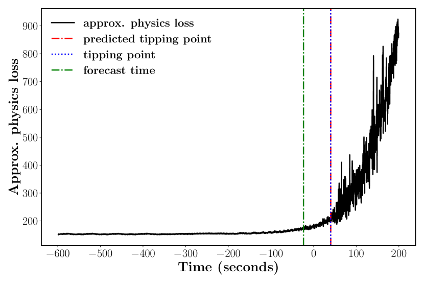
(a) $\eta=1$

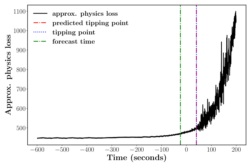
(b) $\eta=3$

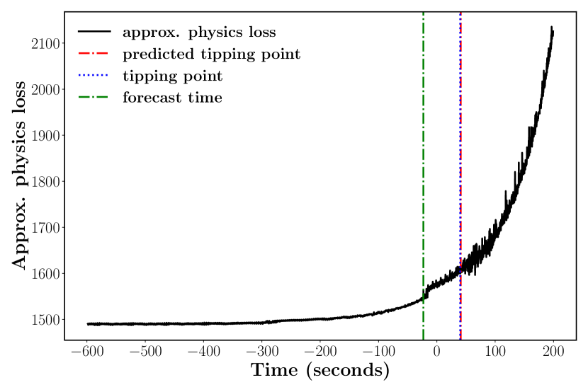
(c) $\eta=10$

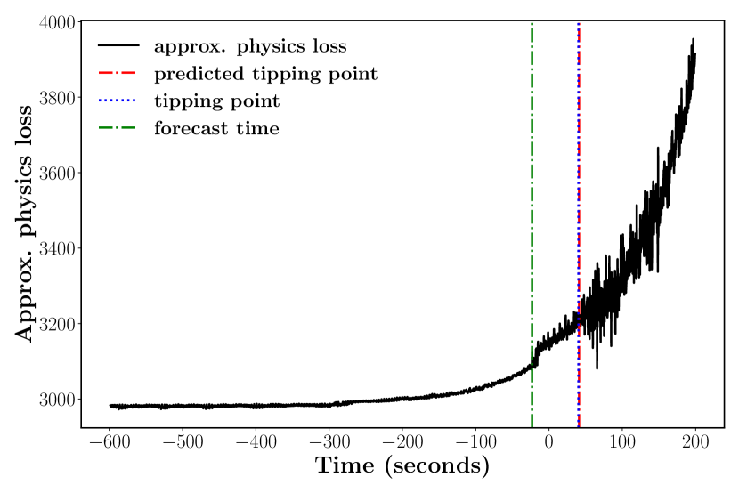
(d) $\eta=20$

Figure 8: Lorenz-63 tipping point forecasting performance $64$ seconds ahead using approximate physical constraints, where $\eta$ is the perturbation on the ODE parameters for the physical law. Our framework is capable of forecasting the tipping points with very low error even with large perturbations $\eta$. A false positive rate of $\alpha=\varepsilon\approx 0.03$ is used, where $\varepsilon$ is discussed in Section 5.

In this section, we investigate our method’s performance in tipping point forecasting using approximate physics constraints. For instance, such a setting may occur when certain coefficients in a PDE or ODE are known only approximately. In this section, we consider this example of approximate physics for the nonstationary Lorenz-63 system, where we evaluate our proposed framework’s capability of forecasting tipping points under different perturbations of the ODE parameters. Specifically, we once again define the physics loss as in Eq. 16, but in this case, we redefine $\widehat{\dot{u}}(t)$ by replacing $\sigma,\rho(t),\beta$ with $\tilde{\sigma}=\sigma+\eta,\tilde{\rho}(t)=\rho(t)+\eta,\tilde{\beta}=\beta+\eta$, respectively, where $\eta$ is some fixed perturbation.

We use the same experimental setup and as in Section A.2. As shown in Fig. 8, our proposed framework is robust to perturbations in the physical constraints and is able to forecast tipping points with very low error far in advance. This is particularly useful for real-world scenarios in which only approximate physical laws are known for a given system.

In particular, we observe that with even approximate physical knowledge of the underlying system, the notion of using the physics loss to verify the correctness of the model’s predictions does not break down. This can be observed in Figures 8(c) and 8(d), where a “bump” in the approximate physics loss can be seen at the forecast time, signaling the shift in distribution of the underlying dynamics.

Appendix B Background on simplified cloud cover model

The model developed in [5, 6] is an extension of a traditional bulk boundary layer model [54], which represents the state of the atmospheric boundary layer and cloud by five coupled ordinary differential equations:

$$\frac{dz_{i}}{dt} =w_{e}(\Delta R,s)-Dz_{i}+w_{\mathrm{vent}}(\mathrm{CF})$$ (18a)

$$\frac{ds}{dt} =\frac{1}{z_{i}}\left[V\cdot(s_{0}(\mathrm{SST})-s)+w_{e}(\Delta R,s)\cdot(s_{+}-s)-\Delta R(\mathrm{CO}_{2},q_{t,+})\right]+s_{\mathrm{exp}}$$ (18b)

$$\frac{dq_{t}}{dt} =\frac{1}{z_{i}}\left[V\cdot(q_{t,0}(\mathrm{SST})-q_{t})+w_{e}(\Delta R,s)\cdot(q_{t,+}-q_{t})\right]+q_{t,\mathrm{exp}}(\mathrm{SST})$$ (18c)

$$\frac{d\mathrm{CF}}{dt} =\frac{f_{\mathrm{CF}}(\mathscr{D})-\mathrm{CF}}{\tau_{\mathrm{CF}}}.$$ (18d)

$$C\frac{d\mathrm{SST}}{dt} =\mathrm{SW}_{\mathrm{net}}(\mathrm{CF})-\mathrm{LW}_{\mathrm{net}}-\mathrm{LHF}(\mathrm{SST},s,q_{t})-\mathrm{SHF}(\mathrm{SST},s)-\mathrm{OHU}.$$ (18e)

The model is formulated such that CO₂ is the only external parameter and all other processes are represented by physically motivated, empirical formulations, with their parameters based on data from satellite observations or high-resolution simulations.

The first three equations physically represent conservation of mass (18a), energy (18b), and water (18c), and the final two are equations for the cloud fraction and the sea surface temperature. In (18a), $z_{i}$ is the depth of the boundary layer [m], $w_{e}$ is the entrainment rate which is itself parameterized as a function of the radiative cooling and the inversion strength, $D$ is the subsidence rate [s^-1], $w_{\mathrm{vent}}$ is an additional additive entrainment term used to parameterize ventilation and mixing from overshooting cumulus convective thermals. In (18b) and (18c), $s$ is the liquid water static energy [J kg^-1] and $q_{t}$ is the total water specific humidity [kg kg^-1]. $V$ is the surface wind speed [m s^-1], $\Delta R$ is the cloud-top radiative cooling per unit density [W m kg^-1], which is a function of CO₂ and H₂O, and $s_{\mathrm{exp}}$ and $q_{t,\mathrm{exp}}$ are export terms representing the effect of large-scale dynamics (synoptic eddies and Hadley circulation) transporting energy and moisture laterally out of the model domain into other regions.

The cloud fraction is modeled as a linear relaxation on timescale $\tau_{\mathrm{CF}}$ to a state $f_{\mathrm{CF}}(\mathscr{D})$ which depends on the degree of decoupling in the boundary layer:

$$f_{\mathrm{CF}}(\mathscr{D}) =\mathrm{CF}_{\mathrm{max}}-\frac{\mathrm{CF}_{\mathrm{max}}-\mathrm{CF}_{\mathrm{min}}}{1+\frac{1}{9}\exp(-m(\mathscr{D}-\mathscr{D}_{c}))}$$ (19a)

$$\mathscr{D} =\left(\frac{\mathrm{LHF}}{\rho\Delta R}\right)\left(\frac{z_{i}-z_{b}}{z_{i}}\right).$$ (19b)

This parameterization is inspired by theoretical and observational work from [55, 56] and parameters $\mathrm{CF_{max}}$, $\mathrm{CF_{min}}$, and $m$ are fit to data from [57, 58, 2].

Equation (18e) is the standard surface energy budget equation for SST. On the left-hand side, $C=\rho_{w}c_{w}H_{w}$ is a heat capacity per unit area, where $\rho_{w}$ and $c_{w}$ are the density and specific heat capacity of water and $H_{w}$ is the depth of the slab ocean. The value of $H_{w}$ is arbitrary (here 1 m): it affects the equilibration time, but not the equilibrium results, which is appropriate given that the forcing is much slower than the equilibration timescale (approx. 50 days). On the right-hand side are the source terms from shortwave and longwave radiation, latent and sensible heat fluxes, and ocean heat uptake. Ocean heat uptake is solved for implicitly such that $\mathrm{SST}=290$ K for $\mathrm{CO}_{2}=400$ ppmv and assumed constant in time.

To generate the data for our experiments, we set the CO₂ forcing to follow

$$\text{CO}_{2}(t)=c_{0}(1+r)^{t}+\sigma W(t),$$ (20)

where $t$ is the time (in years), $W(t)$ is a Wiener process, $c_{0}$ is the initial CO₂ concentration, $r$ is the annual rate of CO₂ increase, and $\sigma$ is the scaling parameter for $W(t)$. We use $c_{0}=400$ ppm, $r=0.1$, and $\sigma=2.5$.

Appendix C Additional results on the KS equation

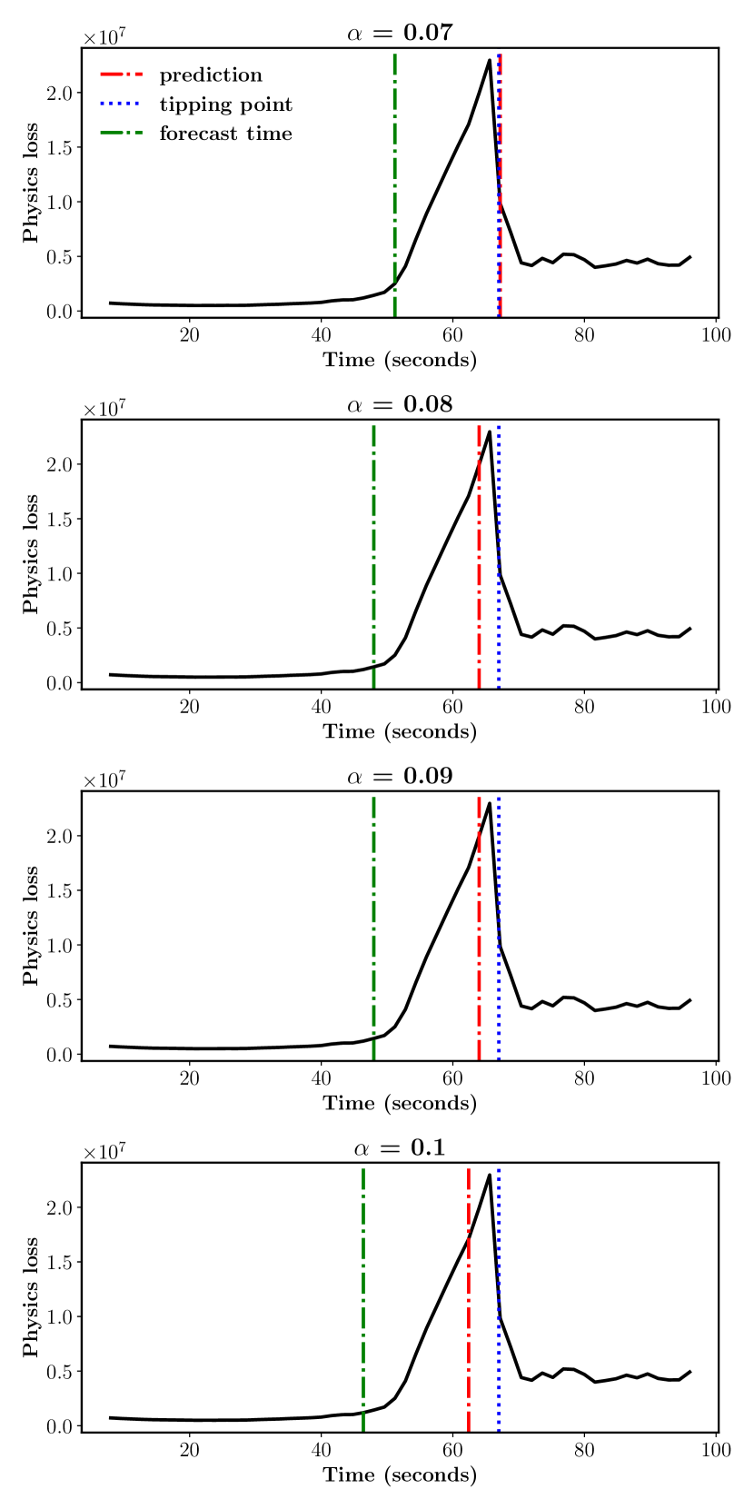
(a) RNO

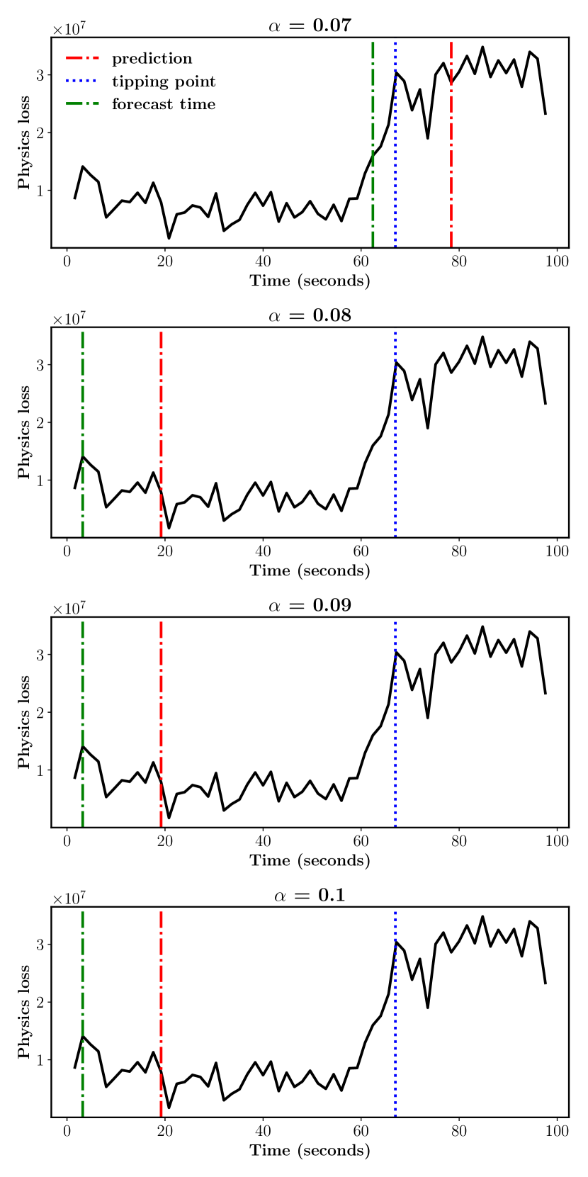
(b) MNO

Figure 9: Comparison of tipping point forecasting performance between RNO and MNO for various false-positive rates $\alpha$ for the KS equation. For all presented $\alpha$, RNO outperforms MNO in tipping point forecasting error.

In this section we compare the performance of RNO in tipping point forecasting with the performance of MNO, for varying values of $\alpha$, the false-positive rate of our method. Note that as shown in Table 2, the relative $L^{2}$ error of RNN on forecasting the evolution of the KS equation is an order of magnitude larger than that of RNO and MNO.

As shown in Figure 9, we observe that for all values of $\alpha$ shown, RNO vastly outperforms MNO in the proximity of tipping point prediction to the true tipping point of the system. This can likely be attributed to the lower performance of MNO in learning the nonstationary system dynamics (see Table 2), which causes MNO to produce fluctuating physics losses even in the pre-tipping regime, whereas RNO has a low, stable physics loss during pre-tipping.

Figure 14(b) compares the critical physics loss threshold $l(\alpha)$ for RNO and MNO when forecasting the KS tipping point $16$ seconds ahead. For lower physics loss thresholds, RNO forecasts the tipping point with much better performance than MNO. As the critical physics loss threshold is increased, the performance of RNO improves slowly, suggesting that the distribution of RNO’s physics loss has little weight on the right tail. In contrast, MNO exhibits the opposite behavior, suggesting that it is less reliable than RNO in learning the non-stationary dynamics. Crucially, we note that comparisons on the accuracy of tipping point predictions between two methods must be made at a fixed false-positive rate $\alpha$ (e.g., see Figure 9). In Figures 14(b) and 14(a), we only seek to compare the distributions of physics loss and each model’s respective ability to learn the underlying dynamics.

Appendix D Additional results on the cloud cover system

D.1 Numerical results in learning non-stationary dynamics

Model	1-step	2-step	4-step	8-step	16-step
RNO	$\mathbf{0.0234}$	$\mathbf{0.0326}$	$\mathbf{0.0449}$	$\mathbf{0.0614}$	$\mathbf{0.0852}$
MNO	$0.0246$	$0.0342$	$0.0472$	$0.0647$	$0.0860$
RNN	$0.0285$	$0.0360$	$0.0481$	$0.0645$	$0.0868$

Table 4: Relative $L^{2}$ errors on the cloud cover system for different $n$-step prediction settings using the experimental setup described in Appendix E.4. RNO outperforms MNO and RNN on every forecasting interval.

Numerical results from our experiments are shown in Table 4. We observe that RNO outperforms MNO and RNN in relative $L^{2}$ error for every $n$-step prediction presented. We find that as the size of the forecasting interval $\Delta T$ (not to be confused with the length of the forecasting window, which is $n\cdot\Delta T$) increases, the performance of RNN worsens substantially. We attribute this to the resolution-dependence of RNN; as the dimensionality of the input (in this case $5\cdot\Delta T$, since the cloud cover system is 5-dimensional) increases, the size of the RNN model must be increased accordingly in order to adequately capture the dynamics of the system. For RNO and MNO, the size of the models need not be increased substantially since the input is interpreted as a function over a larger domain, and the inductive biases of these models allows them to outperform fixed-resolution models such as RNNs.

D.2 Tipping point forecasting using full ODE constraint

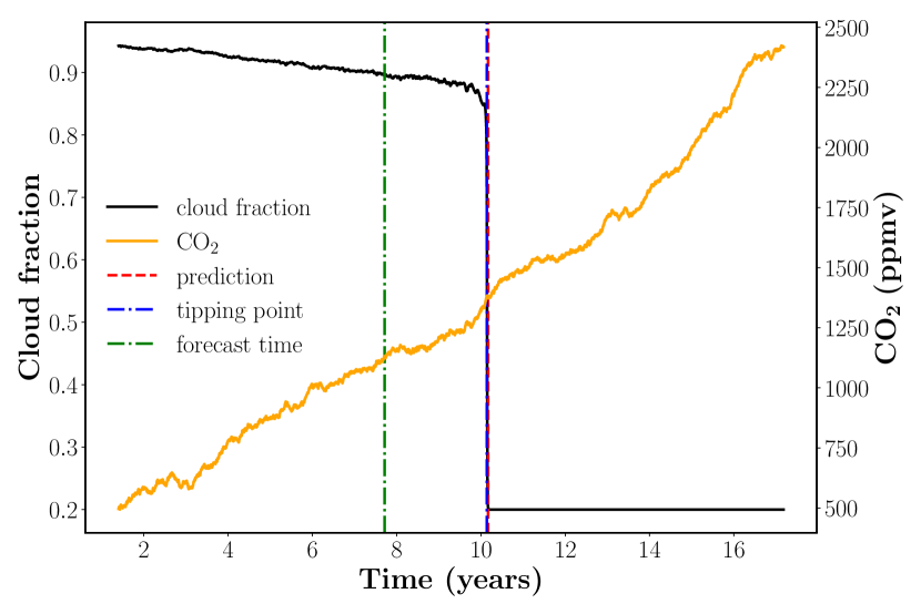
(a) Tipping point forecast w.r.t. cloud fraction

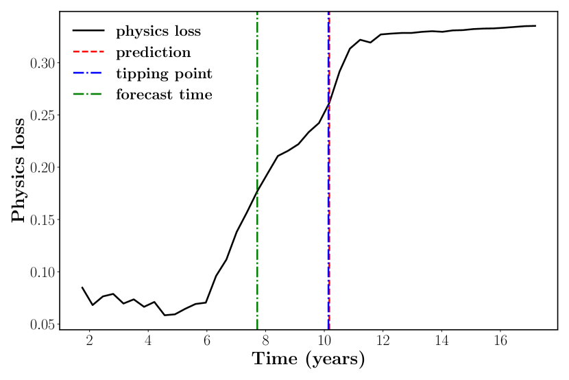
(b) Tipping point forecast w.r.t. partial physics loss

Figure 10: Using the full ODE as the physical constraint, RNO is capable of identifying the true tipping point of the simplified cloud cover system with an error of $0.03$ years, predicting $T=2.45$ years ahead, at $\alpha=0.08$.

In this section, we demonstrate that our proposed method is capable of identifying the tipping point with low error when using the full ODE equation as the physics constraint. Figure 10 shows that our method is capable of forecasting the tipping point far in advance, similarly to Figure 5.

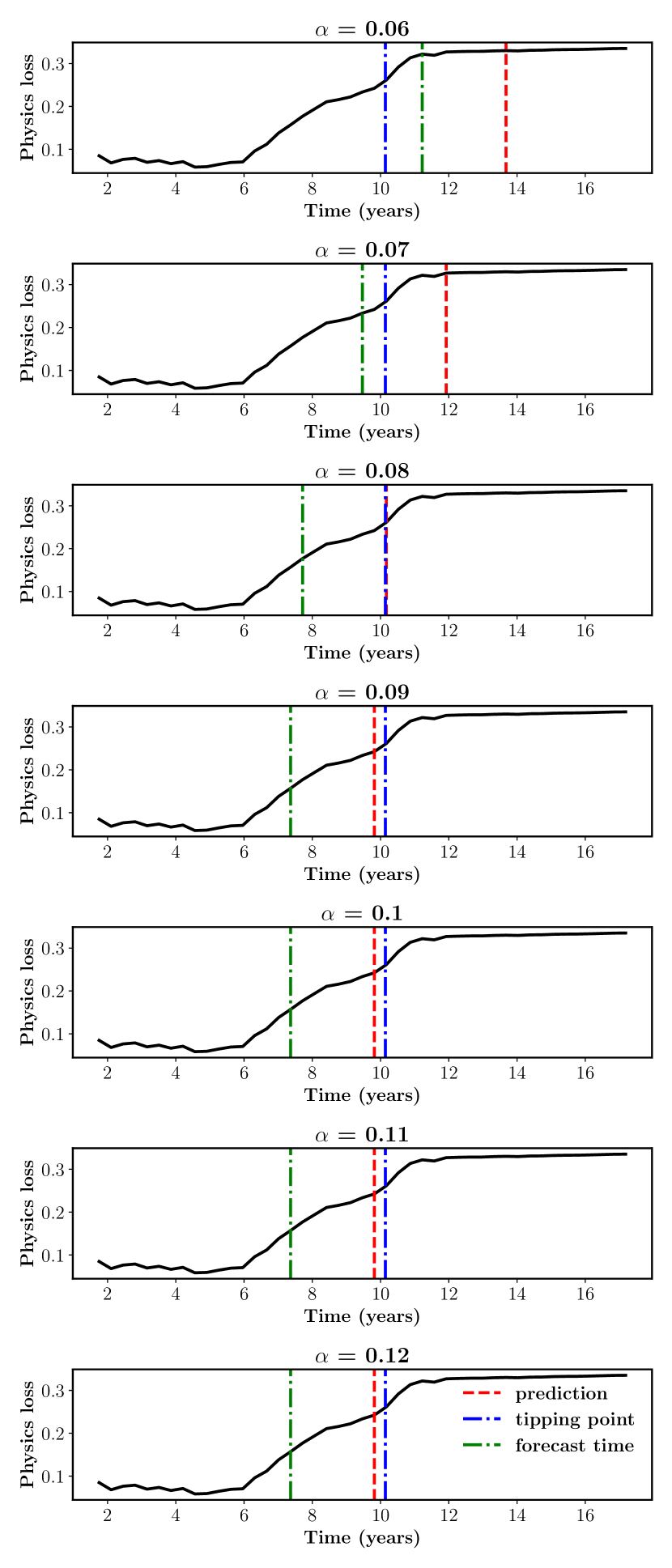
Figure 11: Tipping point forecasting performance for RNO for various false-positive rates $\alpha$ in the simplified cloud cover setting. RNO achieves very low forecasting error for the majority of $\alpha$. Further, RNO achieves approximately zero error for $\alpha=0.08$.

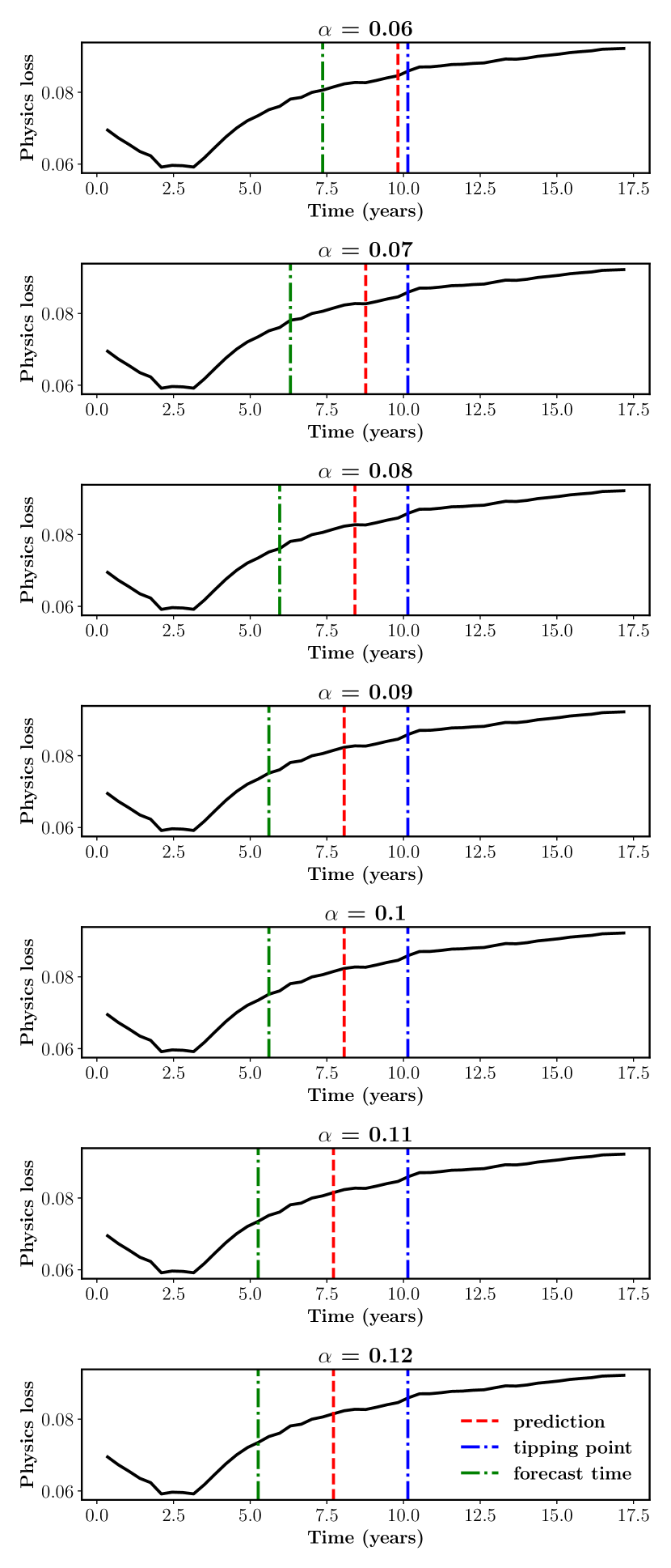
(a) MNO

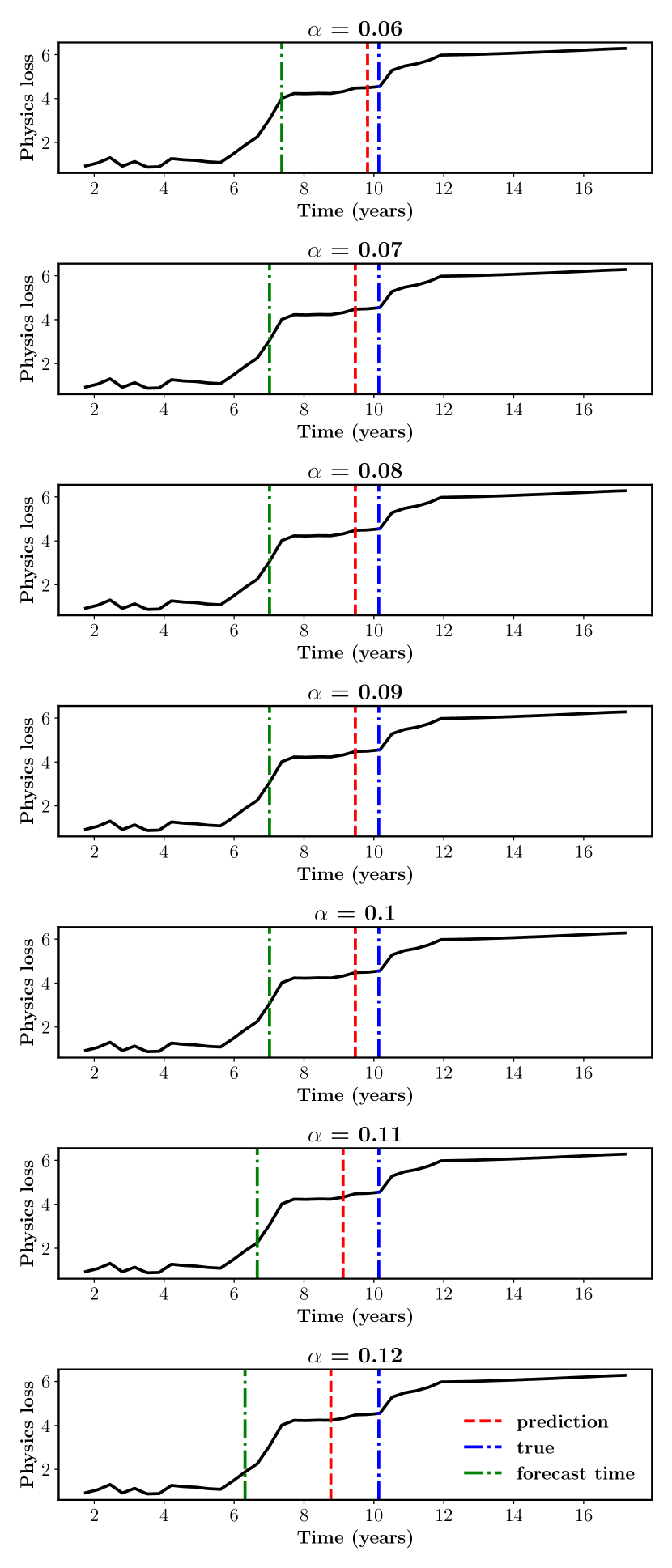
(b) RNN

Figure 12: Comparison of tipping point forecasting performance between MNO and RNN for various false-positive rates $\alpha$ in the simplified cloud cover setting. RNO (in Figure 11) tends to outperform MNO and RNN in tipping point forecasting error for the majority of the $\alpha$.

Similarly to the nonstationary KS setting, we also compare the performance of RNO in tipping point forecasting with MNO and RNN for varying values of false-positive rate $\alpha$ for the simplified cloud cover system (Figures 11 and 12). We observe that RNO overall outperforms RNN and MNO in tipping point forecasting for a variety of false-positive rates $\alpha$. Furthermore, RNO is able to achieve nearly no decrease in error as $\alpha$ increases, for reasonable $\alpha$.

Appendix E Details on numerical experiments

In our RNO experiments, we divide inference into a warm-up phase and a prediction phase. This choice is motivated by the empirical observation that predictions $\widehat{u}_{1},\widehat{u}_{2},\dots$ for small steps $\tau$ tend to be poor because the hidden function $h_{0}(x,t)$ does not contain sufficient information to properly learn complex nonstationary dynamics (which inherently require history). The effect of the warm-up phase is to allow the RNO to construct a useful hidden representation $h_{\tau}$ before its predictions $\widehat{u}_{\tau}$ are used to construct long-time predicted trajectories. We use this procedure both during training and test times.

Furthermore, MNO has achieved state-of-the-art accuracy in forecasting the evolution of stationary dynamical systems by using a neural operator (Section  3) to learn the Markovian solution operator of such systems. As proposed in [10], MNO takes as input the solution at a given time, $u(x,t)$, and outputs $u(x,t+h)$. While the Markovian solution operator holds for some stationary systems [10], non-stationary systems must be handled with more care. As such, we instead compare RNO against a variant of MNO that maps $u(x,[t,t+\Delta T])\mapsto u(x,[t+\Delta T,t+2\Delta T])$. This variant of MNO equips the model with some temporal memory.

E.1 RNN baseline

We use a gated recurrent unit (GRU) [48] architecture for the RNN baseline for the non-stationary Lorenz-63, KS equation, and simplified cloud cover model experiments. We use shallow neural networks to map inputs to a hidden representation that is propagated between time intervals with the GRU, and the final GRU hidden-state is mapped to the output space with another shallow neural network. We observe optimal performance for the RNN when we adopt the same inference process as with RNO, with a warm-up phase and a prediction phase. We observe that the number of time intervals for the warm-up phase needed to achieve acceptable results tends to be higher for RNN than for RNO across our experiments. For instance, we warm up with $10$ intervals for RNN and $5$ for RNO, in both the Lorenz-63 and KS settings. In the cloud cover experiments, we warm up the RNN and RNO both with $5$ time intervals.

In Table 5, we note the effectiveness of multi-step fine-tuning in learning the evolution of longer trajectories in non-stationary systems (compare RNN-8 and RNN-1). However, if multi-step fine-tuning is taken too far (i.e., $M$ is large), we empirically observe convergence to suboptimal local minima (e.g., RNN-12).

E.2 Non-stationary Lorenz-63 system

In our experiments, we generate 15 trajectories using a fourth-order Runge-Kutta method with an integration step of $0.001$. Ten of these trajectories are used for training and the remaining five are used for calibration and testing. Each trajectory is on the range $t\in[-600,200]$. The initial condition for each trajectory is initialized randomly, and the solution is integrated for $50$ integrator seconds and then discarded to allow the system to reach the periodic dynamics. For training and testing, the data is temporally subsampled into a temporal discretization of $0.05$ integrator seconds.

Both the RNO and MNO used for experiments in Section 6 were trained with a width of $48$ and $24$ Fourier modes. See [46] for a description of the hyperparmaters of Fourier layers. We use $L=3$ layers in the RNO and $4$ layers for MNO. We implement the baseline RNN as described in Section E.1, with $3$ layers and a $248$-dimensional hidden state. We set the length of each input/output time interval to $\Delta T=0.32$ seconds. We also fix the number of warm-up samples $N_{\tau}=5$ for RNO experiments. In our experiments, we set $M=12$ and $\lambda_{n}=1$ for all $n$, for the corresponding terms in our data loss (Eq. 14). All models were optimized using Adam [59] with an initial learning rate of $10^{-4}$ and a batch size of $64$. We use a step learning rate scheduler that halves the learning rate every $4000$ weight updates. We train RNO and MNO for $5$ epochs, and we train RNN for $15$ epochs. We pre-train MNO for 50 epochs on one-step prediction.

E.3 Non-stationary KS equation

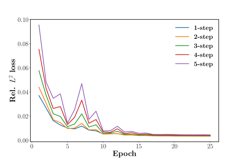
Figure 13: Convergence plot of test relative $L^{2}$ error for RNO trained on the pre-tipping regime of the KS equation. We observe that RNO ultimately converges to near-zero error for all steps.

In our experiments, we generate 200 trajectories of the evolution of the non-stationary KS equation using a time-stepping scheme in Fourier space with a solver time-step of $0.001$. 160 of these trajectories were used for training, 30 of them were used for calibration, and 10 trajectories were used for testing. Each trajectory is defined on the range $t\in[0,100]$. The initial condition is initialized randomly, and the solution is integrated for 100 integrator seconds and then discarded to allow the system to reach periodic dynamics. For training and testing, the data is temporally subsampled into a temporal discretization of $0.1$ integrator seconds. Our models map the previous time interval of length $\Delta T$ to the next time interval of length $\Delta T$. In our model, we use $\Delta T=1.6$ seconds.

Both the RNO and MNO used in our experiments used $20$ Fourier modes across both the spatial and temporal domain. The RNO used has a width of $28$, and MNO used has a width of $32$. We use $L=3$ layers in the RNO and $4$ layers for the MNO. We implement the baseline RNN with $3$ layers and a $512$-dimensional hidden state. We fix the number of warm-up samples $N_{\tau}=5$ for RNO experiments. In our experiments, we set $M=5$ and $\lambda_{n}=1$ for all $n$, for the corresponding terms in our data loss (Eq. 14). All models were optimized using Adam [59] with a batch size of $32$. RNO was trained for $25$ epochs at an initial learning rate of $10^{-3}$, while halving the learning rate every $2000$ weight updates. MNO was pre-trained on one-step prediction for $100$ epochs at a learning rate of $0.005$, halving the learning rate every $200$ weight updates. MNO was then fine-tuned using the loss in Eq. 14 at a learning rate of $10^{-5}$, halving the learning rate every $250$ weight updates. RNN was pre-trained on one-step prediction for $40$ epochs at a learning rate of $0.001$, halving the learning rate every $500$ weight updates. MNO was then fine-tuned using the loss in Eq. 14 at a learning rate of $10^{-5}$, halving the learning rate every $500$ weight updates.

Figure 13 depicts the convergence in test $L^{2}$ error of RNO trained on the KS equation. We obseve that RNO converges to a test $L^{2}$ error close to zero for all steps. Note that at times, training is slightly unstable for $1$-step prediction, and this error propagates to larger degrees for $2$-step, $3$-step, etc., predictions. Empirically, we do not observe that this behavior prevents RNO from adequately learning the multi-step dynamics. In fact, observe that after minor increases in $1$-step error in Figure 13, when the $1$-step error decreases, the multi-step error decreases accordingly.

Model	1-step	2-step	4-step	8-step	16-step	32-step	64-step	128-step
RNO	$\mathbf{0.0053}$	$\mathbf{0.0033}$	$\mathbf{0.0027}$	$\mathbf{0.0028}$	$\mathbf{0.0068}$	$\mathbf{0.0434}$	$\mathbf{0.1549}$	$\mathbf{0.2585}$
RNN-8	$0.0141$	$0.0139$	$0.0173$	$0.0150$	$0.0332$	$0.1096$	$0.2366$	$0.3434$
RNN-12	$0.0532$	$0.0594$	$0.0598$	$0.0618$	$0.0813$	$0.1433$	$0.2231$	$0.3052$
RNN-1	$0.0114$	$0.1644$	$0.2729$	$0.3546$	$0.4030$	$0.4153$	$0.4057$	$0.4006$

Table 5: Relative $L^{2}$ errors on non-stationary Lorenz-63 for different $n$-step prediction settings and number of RNN fine-tuning steps $M$ (denoted “RNN-$M$”). RNO outperforms RNN on every forecasting interval and for every RNN training setup.

E.4 Cloud cover equations

We generate 150 trajectories of the evolution of the non-stationary cloud cover equations [5, 6] described in Appendix B using a 5th order Runge-Kutta Rosenbrock method. We use a integration step of 1 day and solve the system for 20 years for each trajectory. We train our RNO model on 45 trajectories, use 100 for calibration, and 5 for testing. In our models, we set the forecast time length to be $\Delta T=0.36$ years.

The RNO used in our experiments used $64$ Fourier modes across the temporal domain and used a width of $128$. We use $L=5$ layers and multi-step fine-tuning up to $M=10$ steps. The MNO model used $4$ layers, $32$ Fourier modes, and a width of $96$. We implement the baseline RNN with $3$ layers and a $1024$-dimensional hidden state. We fix the number of warm-up samples $N_{\tau}=5$ for RNO experiments. In our experiments, we set $M=10$ and $\lambda_{n}=1$ for all $n$, for the corresponding terms in our data loss (Eq. 14). All models were optimized using Adam [59] with a batch size of $64$. RNO was trained for $25$ epochs at an initial learning rate of $10^{-3}$, while halving the learning rate every $300$ weight updates. Both MNO and RNN were also directly trained using the loss in Eq. 14 at a learning rate of $10^{-3}$, halving the learning rate every $500$ weight updates.

Appendix F Comparisons to prior works

F.1 Comparison to prior machine learning methods

In recent years, there has been a several works using machine learning for tipping point forecasting and prediction [4, 8, 24, 25, 26, 27, 28, 29]. For instance, [8] uses a convolutional long short-term memory (LSTM) model to predict specific types of bifurcations. [28] proposes a similar methodology of classifying critical transitions, smooth transitions, and no transitions. However, such methods are not directly applicable to the large-scale spatiotemporal systems (i.e., on function spaces) that motivate our work and require access to post-tipping data. In another vein of research, reservoir computing (RC)-based methods have been used to learn the dynamics of 3d-Lorenz equation [4, 24, 25, 26, 27]. However, RC approaches do not operate on function spaces and are thus not suitable for many large-scale spatiotemporal scientific computing problems.

More specifically, [4] makes the observation that when a tipping point happens, a well-trained machine learning model on the pre-tipping regime makes a significant error, using this signal as an indicator for tipping points. However, this method requires the use of post-tipping information to compare their model forecasts against. In our work, we extend this observation into our proposed tipping point forecasting method that does not require post-tipping data. Instead, we compare our forecast against the physics constraints or differential equations driving the underlying dynamics, so our method does not require post-tipping data.

Among other reservoir computing works, [25] trains a data-driven reservoir model on pre-tipping dynamics, conditioning the model on certain values of a bifurcation-inducing external parameter. While this method appears successful for simpler toy systems, for real-world systems (e.g., climate) there may be a variety of external parameters that may affect the dynamics of a non-stationarity system, which may be difficult to estimate and identify. [26] also uses reservoir computing but requires access to the full ground-truth system, which may be unknown in real-world systems. In contrast, our method can operate on partial or approximate physics knowledge of the underlying system. [27] also presents a method for tipping point prediction using reservoir computing, but this method suffers from the same scalability concerns of reservoir computing and also requires tipping points to be in the training set, both of which are addressed by our method.

In another realm of methods, [29] introduces an adversarial framework for tipping point prediction. However, this framework requires the querying of an oracle, which is extremely computationally expensive in large-scale spatiotemporal systems of interest.

F.2 Comparisons with traditional early warning signals

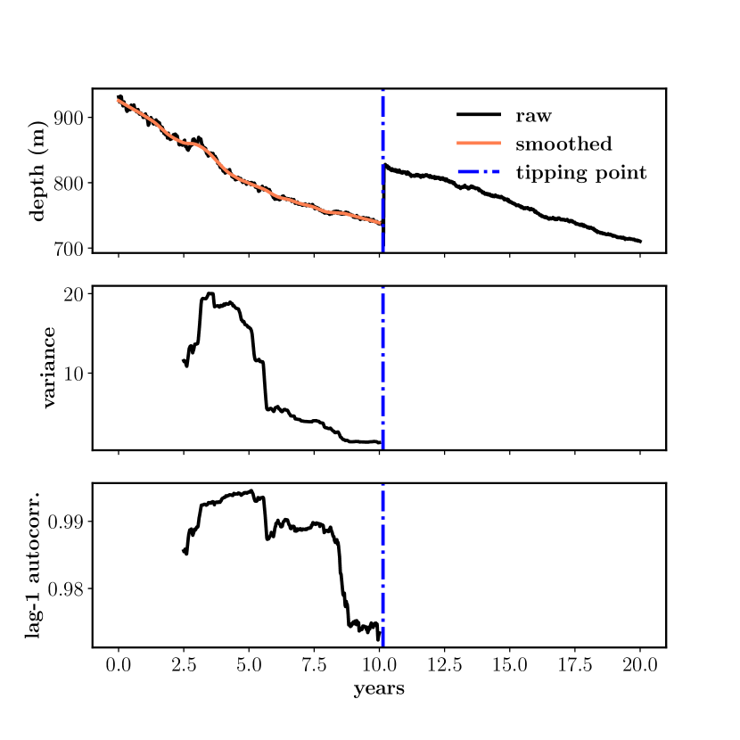
(a) Boundary layer depth

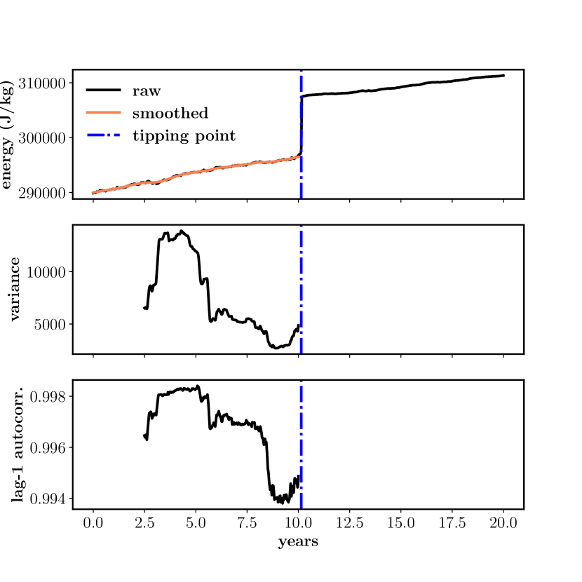
(b) Liquid water static energy

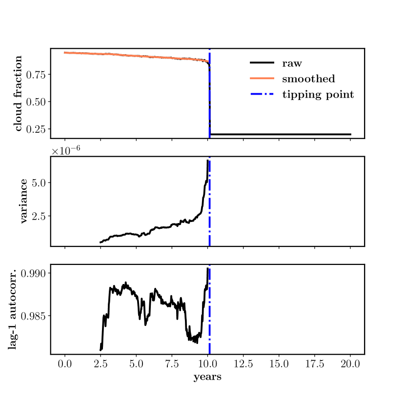
(c) Cloud fraction

Figure 15: Variance and lag-1 autocorrelation applied as early warning signals to forecast impending tipping points in the surrogate cloud cover system. Kendall’s $\tau$ values for (a) variance: $-0.83$, autocorrelation: $-0.48$, (b) variance: $-0.69$, autocorrelation: $-0.59$, and (c) variance: $0.89$, autocorrelation: $-0.33$. Despite approaching a tipping point, autocorrelation did not tend to increase. Only the variance of cloud fraction increased.

To analyze the ability of traditional early warning signals (EWS) to predict tipping points beyond simple well-studied systems, we apply EWS to the cloud cover system [5, 6] in our experiments. In particular, prior works have found that for some systems, increases in variance and autocorrelation are associated with critical slowing down, a phenomenon of slow recovery from perturbations for some systems approaching bifurcation-induced tipping points [7, 60]. As such, we compute the variance and lag-1 autocorrelation using the methods in [60] for each of the five variables in the cloud cover system (see Appendix B for background). The variance and autocorrelation for three of these variables is shown in Figure 15.

Despite autocorrelation and variance being established indicators of tipping phenomena in some systems, we observe that in this real-world system, autocorrelation never has a positive Kendall $\tau$, and variance only has a positive Kendall $\tau$ in the cloud fraction setting. These results suggest that traditional EWS are not reliable as general indicators of tipping phenomena.

We follow the methodology described in [60], and we compute the variance and autocorrelation using the ewstools package [61]. We smooth each univariate time-series using LOWESS smoothing with a span of $0.1$ times the length of the trajectory. We compute lag-1 autocorrelation and variance in rolling windows of length $0.25$ times the length of the trajectory.

Appendix G Technical discussion and analysis of methods

G.1 Memory and inference times

The details for the best-performing RNO and MNO models in each of the experimental settings are provided in Appendix E. In this section we discuss and compare the memory usage and the inference times of RNO and MNO. Timing benchmarks were performed on one NVIDIA P100 GPU with 16 GB of memory.

In general comparisons of RNO and MNO with the same number of layers, Fourier modes, and width, RNO tends to have a significantly larger memory footprint, since all of the gating operations are implemented with Fourier integral operators. However, in situations where memory may be scarce, weight-sharing or factorization methods can be used to vastly reduce memory footprint [62]. Mixed-precision neural operators [63] can also be used to dramatically decrease memory usage and inference times. Apart from the additional Fourier layers for the gating operations, RNO inference has a warm-up period of $N_{\tau}$ steps to achieve a reasonable hidden state representation. This warm-up period scales with $O(N_{\tau})$, since the computation is computed serially. Despite RNO’s longer inference times compared to MNO, we find that these inference times are still much faster than the numerical solvers for a variety of applications, particularly for larger-scale spatiotemporal problems.

For the non-stationary Lorenz-63 setting, our RNO model and MNO model both used $24$ Fourier modes and had a width of $48$. The respective memory usages are 8.1 MB and 1.9 MB, respectively. The respective inference times to generate an entire trajectory is 30.8 seconds and 11.1 seconds, respectively (averaged over 10 instances). While RNO is slower than MNO, it is still significantly faster than the numerical solver, which takes around 90 seconds to generate each trajectory.

For the non-stationary KS equation, we compare RNO and MNO models with $20$ Fourier modes across both time and space and a width of $28$. The respective memory usages are about 90 MB and 7 MB, and the respective inference times to generate a full trajectory are about 1.3 seconds and 0.3 seconds (both averaged over 100 instances). These are both significantly faster than the numerical solver, which takes about 19 seconds to simulate one trajectory.

For the simplified cloud cover experiments, the best-performing RNO model used $64$ Fourier modes and had a width of $128$, whereas the best-performing MNO model used $32$ Fourier modes and had a width of $96$. The corresponding memory usages are 254 MB and 10 MB, respectively. However, note that while these models are the best-performing for their architecture, they do not have the same hyperparameters. MNO with $64$ modes and width $128$ has a memory footprint of 34 MB. The inference time to generate an entire trajectory for RNO is 1.068 seconds, and for MNO the inference time is 0.223 seconds, averaged over 100 instances. Note that these are both orders of magnitude faster than the numerical solver, which takes about 100 seconds to generate an entire trajectory.

G.2 On the choice of hyperparameters for RNO

The primary hyperparameters of our proposed RNO model is $L$, the number of RNO layers, the number of Fourier modes across each dimension of the input, the width (i.e., co-dimension) of each RNO layer, $N_{\tau}$, the number of warm-up intervals, and $M$, the number of auto-regressive steps used during training.

In general, RNO’s $L$ and width is analogous to the depth and width of standard neural networks, or the number of layers and dimensionality of the hidden state in RNN’s. Increasing $L$ allows for more non-linear and expressive mappings to be learned, and the number of parameters in the model increases linearly with $L$. In general, under our implementation we observe that increasing $L$ beyond $5$ or $10$ layers does not confer additional benefits for the systems studied in this paper. We also observe that increasing the width of RNO rarely improves performance significantly, only marginally, if at all.

The number of Fourier modes necessary depends heavily on the underlying dynamics of the data. For instance, for highly turbulent and chaotic fluid flows, a large of number of modes is useful to effectively parameterize and capture high-frequency information. On the other hand, for laminar fluid flows, a large number of Fourier modes may not be necessary.

Adjusting the optimal number of auto-regressive steps $M$ used during training is a trade-off between ease of training and performance (in $L^{2}$ error) on longer time horizons. For large values of $M$, optimization may be difficult and complicated training policies (e.g., progressive steps of pre-training for some $\tilde{M}<M$, then fine-tuning at $M$, etc.) may be necessary to improve performance. However, we find that using some $M>1$ is crucial to achieving good long-term performance. This trade-off can be observed in Table 5. In general, the choice of $M$ may also depend on the system and the goals for the learned surrogate model. For instance, for highly chaotic systems, large $M$ are less likely to provide benefit over smaller $M$, since chaotic systems tend to quickly decorrelate from the past, making precise long-term predictions very challenging [10].

Finally, the choice of the number of warm-up intervals $N_{\tau}$ also depends on the degree of non-stationarity of the system. For stationary Markovian systems, no memory warm-up is needed, in principle, so $N_{\tau}=0$. For highly non-stationary systems (especially those with many latent variables), increasing $N_{\tau}$ can lead to an improvement in model performance. Also, for chaotic systems that decorrelate from the past quickly, large values of $N_{\tau}$ are likely to not bring better performance. In general, we find that $N_{\tau}$ need not be very large; values between 3 and 10 appear to work well for most systems. We also observe that RNO performance appears to be quite robust to $N_{\tau}$, and tuning this hyperparameter often does not bring significant changes in performance.

G.3 Limitations and discussion of proposed methods

As with all data-driven methods, the performance of RNO depends on its training data. On one hand, data-driven approaches are flexible, unconstrained, and have been shown to learn complex dynamics purely from data [10, 64]. On the other hand, purely data-driven approaches often lack theoretical guarantees; in the realm of scientific computing such useful guarantees may be adhering to physically-meaningful conservation laws, for instance.

Despite lacking many theoretical guarantees, our proposed conformal prediction method is capable of quantifying the distribution of model error with respect to the physics loss. That is, our method does not assume that the data-driven RNO (or other data-driven surrogate model) follows physical constraints perfectly in the pre-tipping regime. Using our rigorous proposed uncertainty quantification method, our tipping point prediction method is robust to model errors.

Since RNO is purely data-driven, it can, in principle, be applied to learning the dynamics of arbitrary dynamical systems. For stationary dynamical systems, it is possible for RNO to learn to ignore historical information and thus to simplify to MNO. Unfortunately, if data is sparse or of low-resolution, it may be difficult for RNO to generalize and truly learn the underlying evolution operator of the system. Providing a heuristic rule-of-thumb for the minimum resolution of the training data that RNO needs to adequately learn the dynamics is difficult; this largely depends on the dynamics of the system in question. In general, providing training data at which the underlying physics is not resolved introduces an ill-posed learning problem. On the question of minimum amounts of training data, we find empirically that simple dynamics can be learned with $O(1000)$ training pairs, whereas complex dynamics may need $O(10000)$ training pairs to adequately learn. This is a very coarse estimate derived from our experimental settings and may not generalize to arbitrary systems.

References

- Lemoine and Traeger [2014] Derek Lemoine and Christian Traeger. Watch your step: optimal policy in a tipping climate. American Economic Journal: Economic Policy, 6(1):137–166, 2014.
- Schneider et al. [2019] Tapio Schneider, Colleen M Kaul, and Kyle G Pressel. Possible climate transitions from breakup of stratocumulus decks under greenhouse warming. Nature Geoscience, 12(3):163–167, 2019.
- Rumelhart et al. [1985] David E Rumelhart, Geoffrey E Hinton, and Ronald J Williams. Learning internal representations by error propagation. Technical report, California Univ San Diego La Jolla Inst for Cognitive Science, 1985.
- Patel and Ott [2022] Dhruvit Patel and Edward Ott. Using machine learning to anticipate tipping points and extrapolate to post-tipping dynamics of non-stationary dynamical systems. arXiv preprint arXiv:2207.00521, 2022.
- Singer and Schneider [2023a] Clare E. Singer and Tapio Schneider. Stratocumulus-cumulus transition explained by bulk boundary layer theory. J. Climate (in review), 2023a. doi: 10.22541/essoar.168167352.24863390/v1.
- Singer and Schneider [2023b] Clare E. Singer and Tapio Schneider. CO2-driven stratocumulus cloud breakup in a bulk boundary layer model. J. Climate (in review), 2023b. doi: 10.22541/essoar.168167204.45220772/v1.
- Scheffer et al. [2009a] Marten Scheffer, Jordi Bascompte, William A Brock, Victor Brovkin, Stephen R Carpenter, Vasilis Dakos, Hermann Held, Egbert H Van Nes, Max Rietkerk, and George Sugihara. Early-warning signals for critical transitions. Nature, 461(7260):53–59, 2009a.
- Bury et al. [2021] Thomas M Bury, RI Sujith, Induja Pavithran, Marten Scheffer, Timothy M Lenton, Madhur Anand, and Chris T Bauch. Deep learning for early warning signals of tipping points. Proceedings of the National Academy of Sciences, 118(39):e2106140118, 2021.
- Kovachki et al. [2021] Nikola Kovachki, Zongyi Li, Burigede Liu, Kamyar Azizzadenesheli, Kaushik Bhattacharya, Andrew Stuart, and Anima Anandkumar. Neural operator: Learning maps between function spaces. arXiv preprint arXiv:2108.08481, 2021.
- Li et al. [2022] Zongyi Li, Miguel Liu-Schiaffini, Nikola Kovachki, Kamyar Azizzadenesheli, Burigede Liu, Kaushik Bhattacharya, Andrew Stuart, and Anima Anandkumar. Learning chaotic dynamics in dissipative systems. Advances in Neural Information Processing Systems, 35:16768–16781, 2022.
- Ashwin et al. [2012] Peter Ashwin, Sebastian Wieczorek, Renato Vitolo, and Peter Cox. Tipping points in open systems: bifurcation, noise-induced and rate-dependent examples in the climate system. Philosophical Transactions of the Royal Society A: Mathematical, Physical and Engineering Sciences, 370(1962):1166–1184, 2012.
- Lenton et al. [2008] Timothy M Lenton, Hermann Held, Elmar Kriegler, Jim W Hall, Wolfgang Lucht, Stefan Rahmstorf, and Hans Joachim Schellnhuber. Tipping elements in the earth’s climate system. Proceedings of the national Academy of Sciences, 105(6):1786–1793, 2008.
- Armstrong McKay et al. [2022] David I. Armstrong McKay, Arie Staal, Jesse F. Abrams, Ricarda Winkelmann, Boris Sakschewski, Sina Loriani, Ingo Fetzer, Sarah E. Cornell, Johan Rockström, and Timothy M. Lenton. Exceeding 1.5°C global warming could trigger multiple climate tipping points. Science, 377(6611):eabn7950, 2022. ISSN 0036-8075, 1095-9203. doi: 10.1126/science.abn7950.
- Wang et al. [2023] Seaver Wang, Adrianna Foster, Elizabeth A. Lenz, John D. Kessler, Julienne C. Stroeve, Liana O. Anderson, Merritt Turetsky, Richard Betts, Sijia Zou, Wei Liu, William R. Boos, and Zeke Hausfather. Mechanisms and Impacts of Earth System Tipping Elements. Reviews of Geophysics, 61(1):e2021RG000757, 2023. ISSN 8755-1209, 1944-9208. doi: 10.1029/2021RG000757.
- Rahmstorf [2006] Stefan Rahmstorf. Thermohaline ocean circulation. Encyclopedia of quaternary sciences, 5, 2006.
- Bonan et al. [2022] David B Bonan, Andrew F Thompson, Emily R Newsom, Shantong Sun, and Maria Rugenstein. Transient and equilibrium responses of the atlantic overturning circulation to warming in coupled climate models: The role of temperature and salinity. Journal of Climate, 35(15):5173–5193, 2022.
- Rind et al. [2018] David Rind, Gavin A Schmidt, Jeff Jonas, Ron Miller, Larissa Nazarenko, Max Kelley, and Joy Romanski. Multicentury instability of the atlantic meridional circulation in rapid warming simulations with giss modele2. Journal of Geophysical Research: Atmospheres, 123(12):6331–6355, 2018.
- Mengel and Levermann [2014] M. Mengel and A. Levermann. Ice plug prevents irreversible discharge from east antarctica. Nature Climate Change, 4:451–455, 2014. doi: 10.1038/nclimate2226.
- Favier et al. [2014] Lionel Favier, Gael Durand, Stephen L Cornford, G Hilmar Gudmundsson, Olivier Gagliardini, Fabien Gillet-Chaulet, Thomas Zwinger, AJ Payne, and Anne M Le Brocq. Retreat of pine island glacier controlled by marine ice-sheet instability. Nature Climate Change, 4(2):117–121, 2014.
- Seroussi et al. [2014] H Seroussi, M Morlighem, E Rignot, J Mouginot, E Larour, M Schodlok, and A Khazendar. Sensitivity of the dynamics of pine island glacier, west antarctica, to climate forcing for the next 50 years. The Cryosphere, 8(5):1699–1710, 2014.
- Joughin et al. [2021] Ian Joughin, Daniel Shapero, Pierre Dutrieux, and Ben Smith. Ocean-induced melt volume directly paces ice loss from pine island glacier. Science advances, 7(43):eabi5738, 2021.
- Koven et al. [2015] Charles D Koven, EAG Schuur, Christina Schädel, TJ Bohn, EJ Burke, Guangsheng Chen, Xiaodong Chen, Philippe Ciais, Guido Grosse, Jennifer W Harden, et al. A simplified, data-constrained approach to estimate the permafrost carbon–climate feedback. Philosophical Transactions of the Royal Society A: Mathematical, Physical and Engineering Sciences, 373(2054):20140423, 2015.
- Miner et al. [2022] Kimberley R Miner, Merritt R Turetsky, Edward Malina, Annett Bartsch, Johanna Tamminen, A David McGuire, Andreas Fix, Colm Sweeney, Clayton D Elder, and Charles E Miller. Permafrost carbon emissions in a changing arctic. Nature Reviews Earth & Environment, 3(1):55–67, 2022.
- Patel et al. [2021] Dhruvit Patel, Daniel Canaday, Michelle Girvan, Andrew Pomerance, and Edward Ott. Using machine learning to predict statistical properties of non-stationary dynamical processes: System climate, regime transitions, and the effect of stochasticity. Chaos: An Interdisciplinary Journal of Nonlinear Science, 31(3):033149, 2021.
- Kong et al. [2021] Ling-Wei Kong, Hua-Wei Fan, Celso Grebogi, and Ying-Cheng Lai. Machine learning prediction of critical transition and system collapse. Physical Review Research, 3(1):013090, 2021.
- Lim et al. [2020] Soon Hoe Lim, Ludovico Theo Giorgini, Woosok Moon, and John S Wettlaufer. Predicting critical transitions in multiscale dynamical systems using reservoir computing. Chaos: An Interdisciplinary Journal of Nonlinear Science, 30(12):123126, 2020.
- Li et al. [2023] Xin Li, Qunxi Zhu, Chengli Zhao, Xuzhe Qian, Xue Zhang, Xiaojun Duan, and Wei Lin. Tipping point detection using reservoir computing. Research, 6:0174, 2023.
- Deb et al. [2022] Smita Deb, Sahil Sidheekh, Christopher F Clements, Narayanan C Krishnan, and Partha S Dutta. Machine learning methods trained on simple models can predict critical transitions in complex natural systems. Royal Society Open Science, 9(2):211475, 2022.
- Sleeman et al. [2023] Jennifer Sleeman, David Chung, Anand Gnanadesikan, Jay Brett, Yannis Kevrekidis, Marisa Hughes, Thomas Haine, Marie-Aude Pradal, Renske Gelderloos, Chace Ashcraft, et al. A generative adversarial network for climate tipping point discovery (tip-gan). arXiv preprint arXiv:2302.10274, 2023.
- Hersbach et al. [2020] Hans Hersbach, Bill Bell, Paul Berrisford, Shoji Hirahara, András Horányi, Joaquín Muñoz-Sabater, Julien Nicolas, Carole Peubey, Raluca Radu, Dinand Schepers, et al. The era5 global reanalysis. Quarterly Journal of the Royal Meteorological Society, 146(730):1999–2049, 2020.
- Shafer and Vovk [2008] Glenn Shafer and Vladimir Vovk. A tutorial on conformal prediction. Journal of Machine Learning Research, 9(3), 2008.
- Dvoretzky et al. [1956] Aryeh Dvoretzky, Jack Kiefer, and Jacob Wolfowitz. Asymptotic minimax character of the sample distribution function and of the classical multinomial estimator. The Annals of Mathematical Statistics, pages 642–669, 1956.
- Massart [1990] Pascal Massart. The tight constant in the dvoretzky-kiefer-wolfowitz inequality. The annals of Probability, pages 1269–1283, 1990.
- Ashwin and Newman [2021] Peter Ashwin and Julian Newman. Physical invariant measures and tipping probabilities for chaotic attractors of asymptotically autonomous systems. The European Physical Journal Special Topics, 230(16):3235–3248, 2021.
- Kaszás et al. [2019] Bálint Kaszás, Ulrike Feudel, and Tamás Tél. Tipping phenomena in typical dynamical systems subjected to parameter drift. Scientific reports, 9(1):1–12, 2019.
- Scheffer et al. [2009b] Marten Scheffer, Jordi Bascompte, William A. Brock, Victor Brovkin, Stephen R. Carpenter, Vasilis Dakos, Hermann Held, Egbert H. van Nes, Max Rietkerk, and George Sugihara. Early-warning signals for critical transitions. Nature, 461(7260):53–59, 2009b. ISSN 0028-0836. doi: 10.1038/nature08227.
- Lenton [2011a] Timothy M. Lenton. Early warning of climate tipping points. Nature Climate Change, 1(4):201–209, 2011a. ISSN 1758-678X. doi: 10.1038/nclimate1143.
- Scheffer et al. [2012] Marten Scheffer, Stephen R. Carpenter, Timothy M. Lenton, Jordi Bascompte, William Brock, Vasilis Dakos, Johan van de Koppel, Ingrid A. van de Leemput, Simon A. Levin, Egbert H. van Nes, Mercedes Pascual, and John Vandermeer. Anticipating Critical Transitions. Science, 338(6105):344–348, 2012. ISSN 0036-8075. doi: 10.1126/science.1225244.
- Lenton [2011b] Timothy M Lenton. Early warning of climate tipping points. Nature climate change, 1(4):201–209, 2011b.
- Ditlevsen and Johnsen [2010] Peter D Ditlevsen and Sigfus J Johnsen. Tipping points: Early warning and wishful thinking. Geophysical Research Letters, 37(19), 2010.
- Gopakumar et al. [2023] Vignesh Gopakumar, Stanislas Pamela, and Lorenzo Zanisi. Fourier-rnns for modelling noisy physics data. arXiv preprint arXiv:2302.06534, 2023.
- Rubanova et al. [2019] Yulia Rubanova, Ricky TQ Chen, and David K Duvenaud. Latent ordinary differential equations for irregularly-sampled time series. Advances in neural information processing systems, 32, 2019.
- Habiba and Pearlmutter [2020] Mansura Habiba and Barak A Pearlmutter. Neural ordinary differential equation based recurrent neural network model. In 2020 31st Irish signals and systems conference (ISSC), pages 1–6. IEEE, 2020.
- Liu et al. [2022] Burigede Liu, Margaret Trautner, Andrew M Stuart, and Kaushik Bhattacharya. Learning macroscopic internal variables and history dependence from microscopic models. arXiv preprint arXiv:2210.17443, 2022.
- Li et al. [2020a] Zongyi Li, Nikola Kovachki, Kamyar Azizzadenesheli, Burigede Liu, Kaushik Bhattacharya, Andrew Stuart, and Anima Anandkumar. Neural operator: Graph kernel network for partial differential equations. arXiv preprint arXiv:2003.03485, 2020a.
- Li et al. [2020b] Zongyi Li, Nikola Kovachki, Kamyar Azizzadenesheli, Burigede Liu, Kaushik Bhattacharya, Andrew Stuart, and Anima Anandkumar. Fourier neural operator for parametric partial differential equations. arXiv preprint arXiv:2010.08895, 2020b.
- Rahman et al. [2022] Md Ashiqur Rahman, Zachary E Ross, and Kamyar Azizzadenesheli. U-no: U-shaped neural operators. arXiv preprint arXiv:2204.11127, 2022.
- Cho et al. [2014] Kyunghyun Cho, Bart Van Merriënboer, Caglar Gulcehre, Dzmitry Bahdanau, Fethi Bougares, Holger Schwenk, and Yoshua Bengio. Learning phrase representations using rnn encoder-decoder for statistical machine translation. arXiv preprint arXiv:1406.1078, 2014.
- Takeuchi et al. [2006] Ichiro Takeuchi, Quoc Le, Timothy Sears, Alexander Smola, et al. Nonparametric quantile estimation. Journal of Machine Learning Research, 7:1231–1264, 2006.
- Huang et al. [2021] Audrey Huang, Liu Leqi, Zachary Lipton, and Kamyar Azizzadenesheli. Off-policy risk assessment in contextual bandits. Advances in Neural Information Processing Systems, 34:23714–23726, 2021.
- Lorenz [1963] Edward N Lorenz. Deterministic nonperiodic flow. Journal of atmospheric sciences, 20(2):130–141, 1963.
- Schneider et al. [2020] Tapio Schneider, Colleen M. Kaul, and Kyle G. Pressel. Solar geoengineering may not prevent strong warming from direct effects of CO2 on stratocumulus cloud cover. Proc. Natl. Acad. Sci., 117(48):30179–30185, 2020. ISSN 10916490. doi: 10.1073/pnas.2003730117.
- Manneville and Pomeau [1979] Paul Manneville and Yves Pomeau. Intermittency and the lorenz model. Physics Letters A, 75(1-2):1–2, 1979.
- Stevens [2006] Bjorn Stevens. Bulk boundary-layer concepts for simplified models of tropical dynamics. Theor. Comput. Fluid Dyn., 20(5-6):279–304, 2006. ISSN 0935-4964. doi: 10.1007/s00162-006-0032-z.
- Bretherton and Wyant [1997] Christopher S. Bretherton and Matthew C Wyant. Moisture transport, lower-tropospheric stability, and decoupling of cloud-topped boundary layers. J. Atmos. Sci., 54:148–167, 1997.
- Chung and Teixeira [2012] D. Chung and J. Teixeira. A simple model for stratocumulus to shallow cumulus cloud transitions. J. Climate, 25(7):2547–2554, 2012. ISSN 0894-8755. doi: 10.1175/JCLI-D-11-00105.1.
- Cesana et al. [2019] Grégory Cesana, Anthony D. Del Genio, and Hélène Chepfer. The cumulus and stratocumulus CloudSat-CALIPSO dataset (CASCCAD). Earth Syst. Sci. Data, 11(4):1745–1764, 2019. ISSN 1866-3516. doi: 10.5194/essd-11-1745-2019.
- Zheng et al. [2021] Youtong Zheng, Yannian Zhu, Daniel Rosenfeld, and Zhanqing Li. Climatology of cloud-top radiative cooling in marine shallow clouds. Geophys. Res. Lett., 48(19):e2021GL094676, 2021. ISSN 0094-8276. doi: 10.1029/2021GL094676.
- Kingma and Ba [2014] Diederik P Kingma and Jimmy Ba. Adam: A method for stochastic optimization. arXiv preprint arXiv:1412.6980, 2014.
- Dakos et al. [2012] Vasilis Dakos, Stephen R Carpenter, William A Brock, Aaron M Ellison, Vishwesha Guttal, Anthony R Ives, Sonia Kéfi, Valerie Livina, David A Seekell, Egbert H van Nes, et al. Methods for detecting early warnings of critical transitions in time series illustrated using simulated ecological data. PloS one, 7(7):e41010, 2012.
- Bury [2023] Thomas M Bury. ewstools: A python package for early warning signals of bifurcations in time series data. Journal of Open Source Software, 8(82):5038, 2023.
- Tran et al. [2021] Alasdair Tran, Alexander Mathews, Lexing Xie, and Cheng Soon Ong. Factorized fourier neural operators. arXiv preprint arXiv:2111.13802, 2021.
- White et al. [2023] Colin White, Renbo Tu, Jean Kossaifi, Gennady Pekhimenko, Kamyar Azizzadenesheli, and Anima Anandkumar. Speeding up fourier neural operators via mixed precision. arXiv preprint arXiv:2307.15034, 2023.
- Pathak et al. [2022] Jaideep Pathak, Shashank Subramanian, Peter Harrington, Sanjeev Raja, Ashesh Chattopadhyay, Morteza Mardani, Thorsten Kurth, David Hall, Zongyi Li, Kamyar Azizzadenesheli, et al. Fourcastnet: A global data-driven high-resolution weather model using adaptive fourier neural operators. arXiv preprint arXiv:2202.11214, 2022.