A Feasibility-Preserved Quantum Approximate Solver for the Capacitated Vehicle Routing Problem

Abstract

The Capacitated Vehicle Routing Problem (CVRP) is an NP-optimization problem (NPO) that arises in various fields including transportation and logistics. The CVRP extends from the Vehicle Routing Problem (VRP), aiming to determine the most efficient plan for a fleet of vehicles to deliver goods to a set of customers, subject to the limited carrying capacity of each vehicle. As the number of possible solutions skyrockets when the number of customers increases, finding the optimal solution remains a significant challenge. Recently, a quantum-classical hybrid algorithm known as Quantum Approximate Optimization Algorithm (QAOA) can provide better solutions in some cases of combinatorial optimization problems, compared to classical heuristics. However, the QAOA exhibits a diminished ability to produce high-quality solutions for some constrained optimization problems including the CVRP. One potential approach for improvement involves a variation of the QAOA known as the Grover-Mixer Quantum Alternating Operator Ansatz (GM-QAOA). In this work, we attempt to use GM-QAOA to solve the CVRP. We present a new binary encoding for the CVRP, with an alternative objective function of minimizing the shortest path that bypasses the vehicle capacity constraint of the CVRP. The search space is further restricted by the Grover-Mixer. We examine and discuss the effectiveness of the proposed solver through its application to several illustrative examples.

I Introduction

The Capacitated Vehicle Routing Problem (CVRP) is an NP-hard combinatorial optimization problem attracted significant attention from both industry and science due to its broad applicability and inherent complexity, since its proposal in [1]. The objective of the CVRP is to find an optimal set of routes for a fleet of vehicles to serve a set of customers, seeking to minimize the time or total distance, etc. The problem can be defined on a graph $G=(V,E)$. We define $V\!=\!\{V_{0},V_{1},\dots,V_{N\!-\!1}\}$ to be the set of vertices, with the vertex $V_{0}$ as the depot, and vertex $V_{i}$, $i\!\in\!\{1,2,\dots,N\!-\!1\}$, signifies the location of the customer $i$ with a certain demand $q_{i}$. $E$ is defined to be a set of directed edges. Each edge $(i,j)\!\in\!E$ has a weight $w_{ij}$, indicating the distance for traveling from customer $i$ to customer $j$. With vehicles having a capacity $Q$ $(Q\!\geqslant\!q_{i})$, the solution comprises a set of routes that meet the following constraints:

• Depot Constraint: All routes must start and end at the depot;

• Customer Visit Constraint: Each customer must be visited exactly once by one of the vehicles;

• Vehicle Capacity Constraint: The total demand of customers along a route must not exceed the capacity of the vehicle.

This paper presents a quantum heuristic method focuses on achieving the solution with the shortest total distance.

Recently, there has been significant progress in quantum computing. A plethora of quantum algorithms has been proposed [2, 3, 4], aiming to achieve computational advantages over their classical counterparts. One of them in solving combinatorial optimization problems is the Quantum Approximate Optimization Algorithm (QAOA) [5] or its variant the Quantum Alternating Operator Ansatz (AOA) [6].

Given a binary assignment combinatorial problem $(F,C)$, the objective is to find the optimal solution $x^{\ast}\!\in F\!\subseteq\{0,1\}^{n}$, corresponding to the minimum of $C(x)$. $n$ denotes the number of required decision bits. The QAOA encodes the solution, using an $n$-qubit parameterized state that evolves from the ground state of the initial Hamiltonian ($H_{M}$) through a trotterized adiabatic time evolution in $p$ steps. The parameters are optimized to force the prepared state to approach the ground state of the cost-based Hamiltonian ($H_{C}$), which encodes the optimal solution to the given problem. Thus, the QAOA gives the approximate solution for the combinatorial optimization problems.

The advantage of the QAOA to solve unconstrained combinatorial problems, such as Max-Cut, is discussed in [7, 8]. However, the QAOA solutions suffer from a low feasible solution ratio for constrained problems whose $F\subsetneqq\{0,1\}^{n}$, with several experimental studies illustrating this limitation even in toy examples [9, 10, 11, 12]. Since the penalty terms are incorporated for infeasible solutions, as shown in Figure 1(a), the energy landscape produced by QAOA has many local minima and barren plateaus in the typical parameter range.

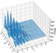
(a) QAOA

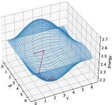
(b) GM-QAOA

Figure 1: The energy landscapes of depth-$1$ 1(a) QAOA and 1(b) GM-QAOA circuits for solving the Traveling Salesman Problem (TSP). The red lines track the optimization process. The optimizer finds the position of the lowest energy state in the GM-QAOA, while it becomes trapped in a local minimum within the QAOA.

The variant AOA aims to preserve the feasibility by specifying a mixing operation according to the constraints. Two recent researches [13, 14] reveal that the state starts from an equal superposition of all feasible states could be beneficial. Following this, [15] provides a general form of mixer that preserves the constraints, known as the Grover-Mixer. As shown in Figure 1(b), the energy landscape of the Grover-Mixer Quantum Alternating Operator Ansatz (GM-QAOA) is smooth, which eases the difficulty of the optimization. However, GM-QAOA requires a preparation unitary for the equal superposition of all feasible states, thereby limiting its range of applications.

In this work, we propose a GM-QAOA solver for the CVRP. The solver ensures feasibility through two key approaches. First, we introduce an $\mathcal{O}(N^{2})$ binary variable encoding of the solution, that enables the application of the preparation unitary for the Grove-Mixer, preserving the customer visit constraint. Concurrently, the solution decoding process is conditionally executed to bypass the vehicle capacity constraint. Considering the cost Hamiltonian also becomes condition-dependent in this scenario, we propose an auxiliary circuit for condition encoding. Incorporating this with other operations, the quantum circuit comprises $\mathcal{O}(pN^{2}(N+(\log_{2}Q)^{2}))$ gates. As a result, our proposed method produces high-quality solutions for the CVRP, as evidenced by our experimental results.

II The Grover-Mixer Quantum Alternating Operator Ansatz

In the QAOA and its variants [5, 6, 13, 15], the initial step typically involves the encoding of the given problem into a quadratic unconstrained binary optimization (QUBO) problem [16] or a higher-order binary optimization (HOBO) problem [17], in the form as:

$$\begin{split}\min_{x\in\{0,1\}^{n}}C(x),\quad C(x)=\sum_{S\subseteq\{0,1,\dots,n-1\}}w_{S}\prod_{i\in S}x_{i},\end{split}$$ (1)

where $x$ is a binary vector of size $n$ that encodes the solution, and $w_{S}$ are the real-valued weights that define the optimization problem. Then, the binary $x_{i}$ is replaced by $(I\!-\!Z_{i})/2$ to yield the cost Hamiltonian,

$$H_{C}=\sum_{S\subseteq\{0,1,,\dots,n-1\}}w_{S}\prod_{i\in S}\frac{I-Z_{i}}{2},$$ (2)

where $Z_{i}$ denotes the Pauli-$Z$ operation acting on the $i^{th}$ qubit. The cost Hamiltonian $H_{C}\!\in\!\mathbb{R}^{2^{n}}$ satisfies $\langle x|H_{C}|x\rangle=C(x)$.

Inspired by adiabatic quantum computing [18], the QAOAs prepare a parameterized state denoted by $|\psi(\boldsymbol{\gamma},\boldsymbol{\beta})\rangle$. This state evolves from an initial state through a series of $p$ repetitions, wherein two distinctive types of operations are employed, the phase separation operation $U_{P}(\gamma)=e^{-i\gamma H_{C}}$ and the mixing operation $U_{M}(\beta)=e^{-i\beta H_{M}}$, as the following formulation,

$$|\psi(\boldsymbol{\gamma},\boldsymbol{\beta})\rangle=\prod_{j=1}^{p}U_{M}(\beta_{j})U_{P}(\gamma_{j})U_{S}|0\rangle^{\otimes n},$$ (3)

where $U_{M}$ is an easy preparable unitary, and the initial state $U_{S}|0\rangle^{\otimes n}$ is the ground state of the $H_{M}$. The depth $p$ is pre-defined. $\boldsymbol{\gamma}\!=\![\gamma_{1},\gamma_{2},\dots,\gamma_{p}]$ and $\boldsymbol{\beta}\!=\![\beta_{1},\beta_{2},\dots,\beta_{p}]$ are trainable parameters. They are tuned to find the ground state of $H_{C}$ by optimizing the expected value $E(\boldsymbol{\gamma},\boldsymbol{\beta})$:

$$E(\boldsymbol{\gamma},\boldsymbol{\beta}) =\langle\psi(\boldsymbol{\gamma},\boldsymbol{\beta})|H_{C}|\psi(\boldsymbol{\gamma},\boldsymbol{\beta})\rangle.$$ (4)

The initial state of the GM-QAOA is an equal superposition of all solutions in the feasible solution set $F$ [15]:

$$U_{S}|0\rangle^{\otimes n}=|F\rangle=\frac{1}{\sqrt{|F|}}\sum_{x\in F}|x\rangle.$$ (5)

$H_{M}$ is defined as $|F\rangle\langle F|$. Thus, the mixing operation has a Grover-like form [2],

$$\begin{split}U_{M}(\beta)&=e^{-i\beta|F\rangle\langle F|}\\ &=U_{S}(I-(1-e^{-i\beta})|0\rangle\langle 0|^{\otimes n})U_{S}^{\dagger},\end{split}$$ (6)

which is composed of $\mathcal{O}(U_{S}+n)$ gates. As proven in [15], the Grover Mixer restricts the search space to $F$, and the states that correspond to an identical objective value have the same amplitude.

The application of the Grover Mixer transforms the issue of seeking the constraint-preserve mixer of the AOA into the pursuit of appropriate $U_{S}$. At present, $U_{S}$ has been polynomially formulated for the unconstrained problems, the permutation-based problems (i.e., problems involving the ordering of elements), and the problems whose feasible set $F$ exactly contains solutions with the same Hamming weight.

III Related Work

Recently, several QUBO formulations have been proposed for the CVRP and its variants. [19] presents a formulation for the CVRP with windows. The solution is encoded using $T\times N\times K$ number of decision bits, where $T$, $N$, and $K$, respectively, represent the numbers of time intervals, customer locations, and vehicles. To preserve the vehicle capacity constraint, they introduce additional bits for capacitated variables. [20, 12] introduce the bits of slack variables to transform the vehicle capacity constraint into an equality constraint. In [21, 9], the binary variables are implemented to represent the decisions associated with the solution edges of VRP and the Multi-depot CVRP.

An alternative approach to the CVRP lies in the 2-Phase-Heuristic [22]. In the first phase, customers are clustered into several groups such that the total demand of each group does not surpass the vehicle’s capacity. The second phase addresses the Traveling Salesman Problem (TSP) within each group. [20] propose a hybrid solution that adopts a classical algorithm [23] for the clustering phase, while the remaining TSPs are solved using quantum annealing [24]. Both phases can be converted into QUBO forms. Specifically, the clustering phase is an adaptation of the Multiple Knapsack problem (MKP). The QUBO forms of the MKP and the TSP are discussed in detail in [25, 20, 26, 10, 12].

The QAOA with penalty terms is anticipated to yield poor-quality results due to the intricate energy landscape. However, there is also no method known to efficiently prepare the equal superposition of all the feasible states for the QUBO-formed CVRP [20, 12]. Meanwhile, the methods to solve the CVRP typically have the vehicle or route number predefined, which in turn narrow the search space. To mitigate these limitations, this study introduces a brand-new formulation for the CVRP. Herein, the solution encoding is divided into two parts: the first represents a permutation of customers, while the second remains unconstrained, serving to transform the routes into cyclic paths, where the combinations encapsulate all potential numbers of routes. Thus, the predetermination of the route number is not required. In addition, we can improve the performance by applying the GM-QAOA.

(a) An example of solution encoding for a $6$-location CVRP.

(b) The decoded solution. The node $(V_{i},q_{i})$ indicates the location of the customer $i$ and the demand $q_{i}$.

Figure 2: Visualization of the proposed problem encoding. Permutation matrix $x$ exhibit a certain order of customer visits, delineated as $[3,4,5,1,2]$. The vehicle returns to the depot before visiting $V_{4}$ and $V_{1}$, as decision bit $y_{2}=1$ and the insufficiency of the vehicle’s capacity at time step $3$ to meet the demand of $V_{1}$.

IV GM-QAOA for CVRP

In this section, we describe the proposed problem encoding and the structure of the quantum circuit.

IV-A The Problem Encoding

The CVRP can be conceptualized as planning the shortest singular route undertaken by one vehicle, permitted to refill its capacity at the depot. While the solution is identified as the collection of sub-routes, each starting and ending at the depot. In this scenario, customers are served sequentially, whereby the order in which customers are visited corresponds to a permutation. For a given CVRP defined on graph $G\!=\!(V,E)$, where $|V|\!=\!N$, a one-hot vector $x_{t}\!\in\!\{0,1\}^{N\!-\!1}$, subject to $\sum_{i=1}^{N-1}x_{t,i}\!=\!1$, is employed to represent the customer being served at time step $t\in\{1,2,\dots,N\!-\!1\}$. $x_{t,i}=1$ signifies that the customer $i$ is visited at time step $t$. Furthermore, considering that each customer is visited exactly once, these one-hot vectors encode different customer numbers. Thus, the feasible space of $x$ is derived as follows:

$$F_{x}=\{ x|\,x\in\{0,1\}^{(N-1)\times(N-1)};$$ (7a)

$$\forall\,t\in\{1,2,\dots,N-1\},\,\sum_{i=1}^{N-1}x_{t,i}=1;$$ (7b)

$$\forall\,i\in\{1,2,\dots,N-1\},\,\sum_{t=1}^{N-1}x_{t,i}=1\},$$ (7c)

where $x$ is defined as a permutation matrix.

The vehicle is granted the option to return to the depot before reaching the customer at time steps ranging from $2$ to $N\!-\!1$. This decision is encoded through another binary string $y\!=\!y_{2}y_{3}\dots y_{N\!-\!1}$, with $y_{t}\!=\!1$ indicating a depot visit between time steps $t\!-\!1$ and $t$. In addition, a depot visit also arises when the current capacity fails to satisfy the demand of the next customer. To address these possibilities, we introduce conditional functions within the process of decoding a solution, as summarized in Algorithm 1, and further elucidated with an example illustrated in Figure 2. Thus, $y$ enjoys an unconstrained feasible space, extending over $F_{y}=\{0,1\}^{N-2}$.

The cost function of the total distance is formulated as follows:

$$C(s)=\sum_{(i,j)\in s}w_{ij},$$ (8)

where $s$ is a decoded solution, and $w_{ij}$ represents the distance traveling from location $V_{i}$ to location $V_{j}$.

Algorithm 1 Solution decoding

Input: Encoding $x,y$; Demands $q$; Capacity $Q$
Output: Solution $s$

1:  $i\leftarrow\arg\max x_{1}$

2:  $s\leftarrow[(0,i)]$

3:  $d\leftarrow q_{i}$

4:  for $t\sim\left[2,3,\dots,|y|+1\right]$ do

5:     $j\leftarrow\arg\max x_{t}$

6:     if $d+q_{j}\leqslant Q$ and $y_{t}=0$ then

7:        append $(i,j)$ to $s$

8:        $d\leftarrow d+q_{j}$

9:     else

10:        append $(i,0)$ to $s$

11:        append $(0,j)$ to $s$

12:        $d\leftarrow q_{j}$

13:     end if

14:     $i\leftarrow j$

15:  end for

16:  append $(i,0)$ to $s$

17:  return $s$

IV-B Preparation Unitary

We employ $(N\!-\!1)$ numbers of $(N\!-\!1)$-qubit quantum registers to encode the permutation matrix $x$. [15] have introduced a preparation unitary $U_{x}$ for preparing the equal superposition of all possible permutations as:

$$|F_{x}\rangle=U_{x}|0\rangle^{\otimes(N-1)^{2}}=\frac{1}{\sqrt{(N-1)!}}\sum_{x\in F_{x}}|x\rangle.$$ (9)

This superposition is constructed register by register, involving the following two key steps. First, the constraint of the register (i.e., (7b) in Equation (7)) under construction is satisfied applying the $\mathcal{O}(N)$ or $\mathcal{O}(N^{2})$ gates controlled by the last register, while preserving the state of other registers. Second, the last register is updated to satisfy the column constraint (i.e., (7c) in Equation (7)). Hence, the superposition can be prepared by utilizing an $\mathcal{O}(N^{3})$ size circuit, see details in [15].

The decision vector $y$ is encoded by an $(N\!-\!2)$-qubit quantum register. As $y$ is unconstrained, the corresponding equal superposition can be prepared using Hadamard gates ($H$), as follows:

$$|F_{y}\rangle=H^{\otimes(N-2)}|0\rangle^{\otimes(N-2)}=\frac{1}{\sqrt{2^{(N-2)}}}\sum_{y\in F_{y}}|y\rangle.$$ (10)

Thus, we have the preparation unitary of the GM-QAOA for the CVRP, as follows:

$$U_{S}=U_{x}\otimes H^{\otimes(N-2)}.$$ (11)

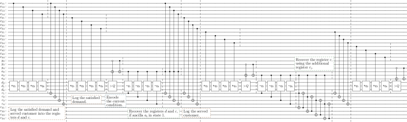
Figure 3: The circuit of condition encoding operation $U_{E}$. The depot visit condition for each time step is stored into the ancilla register $a$, segmented by full-row barriers. Each step consists of four typical procedures separated by partial-row barriers. First, the satisfied demand of the customer is logged into register $d$. Then, register $d$ and decision qubit $y_{t}$ control the flip of $a_{t}$, where $a_{t}\!=\!1$ suggests a depot visit. After that, if such a depot visit occurs, the register $d$ and $c$ are recovered. Finally, the visited customer number is recorded into register $c$.

IV-C Phase Separation Operation

Unlike typical QAOA-based solvers, a direct derivation of the cost Hamiltonian from the cost function is unavailable in our proposal. Instead, we introduce an additional ancilla bit, denoted as $a_{t}$, to signify the condition at each time step $t\!\in\!\{2,3,\dots,N\!-\!1\}$, as follows,

$$a_{t}=\begin{cases}1&\text{if $y_{t}=1$, or capacity insufficiency},\\ 0&\text{otherwise}.\end{cases}$$ (12)

It enables the reformulation of the cost function to be:

$$\mathcal{C}(x,a) =\sum_{i=1}^{N-1}w_{0i}x_{1,i}+\sum_{i=1}^{N-1}w_{i0}x_{N\!-\!1,i}$$ (13a)

$$+\sum_{t=2}^{N-1}[(1-a_{t})\sum_{i,j=1;i\neq j}^{N-1}w_{ij}x_{t\!-\!1,i}x_{t,j}$$ (13b)

$$\qquad+a_{t}\sum_{i,j=1;i\neq j}^{N-1}(w_{i0}x_{t\!-\!1,i}+w_{0j}x_{t,j})].$$ (13c)

Specifically, the terms in (13a) compute the distances of the first and last locations transitioning to or from the depot, respectively. The terms in (13b) and (13c), respectively, represent the distances of two possible routes that the vehicle travels intermediate pair of locations under two conditions, according to Equation (12).

We replace all binary variables $b\!\in\!x,a$ by $(I\!-\!Z_{b})/2$ to obtain the cost Hamiltonian $H_{C}$. Then, we can apply the phase separation operation with $N\!-\!2$ ancilla qubits. The ancilla qubits (register $a$) are entangled with the decision qubits (register $x,y$), using a condition encoding unitary $U_{E}$, as proposed in Section IV-D. The phase separation operation is formulated as follows,

$$U_{P}(\gamma)=U_{E}^{\dagger}e^{-i\gamma H_{C}}U_{E},$$ (14)

where $e^{-i\gamma H_{C}}$ can be decomposed into $\mathcal{O}(N^{2})$ number of CNOT and $z$-axis rotation gates [27].

IV-D Condition Encoding Operation

To encode conditions to register $a$, we introduce another three ancilla registers: $d$, $c$, and $r$. The register $d$ and $c$, respectively containing $\left\lceil\log_{2}(Q\!+\!\max(q)\!+\!1)\right\rceil$ and $N\!-\!1$ qubits, serve to record the satisfied demands and customers in the sub-route. The register $r$ is used to recover register $c$.

As shown in Figure 3, the encoding is processed time step by time step, employing $4$ procedures discussed in the following.

IV-D1 Log the satisfied demand

At each time step $t$, we initially augment register $d$ with the demand of the customer currently being visited. This operation is carried out by employing $N-1$ number of $x_{t,i}$-controlled $\left[+q_{i}\right]$ gates, for all $i\!\in\!\{1,2,\dots,N\!-\!1\}$. As $x_{t}$ preserves hamming weight of 1, only one $\left[+q_{i}\right]$ gate can be activated to add the satisfied demand to $d$. The $\left[+q_{i}\right]$ gate works as follows,

$$\left[+q_{i}\right]_{n}|d\rangle=|(d+q_{i})\ \mathrm{mod}\ 2^{n}\rangle,$$ (15)

where $n$ is the number of qubits acting on and $d$ encodes the satisfied demand in binary.

Suppose $\tilde{q}_{i}\!=\!\tilde{q}_{i,K-1}\dots\tilde{q}_{i,0}$ is a binary representation of $q_{i}$, we can decompose the $\left[+q_{i}\right]_{n}$ gate as,

$$\begin{split}\left[+q_{i}\right]_{n}&=\prod_{k=0,\tilde{q}_{i,k}=1}^{K-1}\left[+2^{k}\right]_{n}\\ &=\prod_{k=0,\tilde{q}_{i,k}=1}^{K-1}\begin{bmatrix}0&I_{2^{k}}\\ I_{2^{n}-2^{k}}&0\end{bmatrix}\\ &=\prod_{k=0,\tilde{q}_{i,k}=1}^{K-1}\left[+1\right]_{n-k}\otimes I_{2^{k}},\end{split}$$ (16)

where $I_{2^{k}}$ denotes a Identity matrix of size $2^{k}$. [28] exhibits a construction that turns $\left[+1\right]_{n}$ into $\mathcal{O}(n)$ Toffoli, CNOT, and Pauli-$X$ gates. The number of $\left[+1\right]$ operations required to generate $\left[+q_{i}\right]$ is tied to the count of ‘1’ present in $\tilde{q}_{i}$. As $q_{i}\leqslant Q$, it is restricted to $\mathcal{O}(\log_{2}Q)$. Hence, this logging operation requires $\mathcal{O}(N(\log_{2}Q)^{2})$ gates.

IV-D2 Encode the condition

The encoding of the condition at time step $t$ is implemented following the logging of satisfied demand. As depicted in Equation (12), $a_{t}$ turns to $1$ when $y_{t}=1$ or in the case of capacity insufficiency. Hence, our first operation involves the deployment of a CNOT gate, designed to flip the state of $a_{t}$ when $y_{t}$ is in state $|1\rangle$.

The register $d$ encodes the sum of the current demand and demands previously satisfied, implying a depot visit when the encoded number exceeds $Q$. To account for all distinct circumstances where $d$ is larger than $Q$, we employ a series of multi-controlled Pauli-$X$ gates to flip $a_{t}$, denoted as,

$$\begin{split}&\left[>\!\displaystyle Q\right]=\prod_{i=0,\tilde{Q}_{i}=0}^{K-1}MCX_{\tilde{Q}_{K\!-\!1}\dots\tilde{Q}_{i+1}1}^{d_{K\!-\!1}d_{K\!-\!2}\dots d_{i}},\\ &(K=\left\lceil\log_{2}(Q\!+\!\max(q)\!+\!1)\right\rceil),\end{split}$$ (17)

where $\tilde{Q}$ is a binary representation of $Q$. $MCX_{cs}^{cq}$ denotes the multi-controlled Pauli-$X$ gate, with $cq$ as the control qubits and $cs$ as the control states of $cq$. A demonstrative example of $\left[>\!\displaystyle Q\right]$ is provided in Figure 4. $\left[>\!\displaystyle Q\right]$ is controlled by $y_{t}$, and can only be activated when $y_{t}$ is in state $|0\rangle$. It prevents a double flip of $a_{t}$ when capacity insufficiency occurs and $y_{t}$ is in state $|1\rangle$.

An $n$-controlled Pauli-$X$ gate can be realized via $\mathcal{O}(n)$ Toffoli, CNOT, and single-qubit gates. Thus, we can implement $\left[>\!\displaystyle Q\right]$ within $\mathcal{O}((\log_{2}Q)^{2})$ size circuit.

Figure 4: The decomposition of $\left[>\!\displaystyle Q\right]$, where $Q\!=\!9$, can be presented in a binary format as ‘01001’. According to Equation (17), the $\left[>\!\displaystyle 9\right]$ can be decomposed into a sequence of three multi-controlled Pauli-$X$ gates. Specifically, the control states for each gate are identified as ‘1’, ‘011’, and ‘0101’, each, respectively, corresponding to control qubits $d_{4}$, $d_{4}d_{3}d_{2}$, and $d_{4}d_{3}d_{2}d_{1}$.

Figure 5: The overall circuit of the CVRP based on the GM-QAOA framework. $x$ and $y$ are the decision registers, supported by the ancilla registers $a$, $d$, $c$, and $r$. $U_{x}$ and $H$ initialize the equal amplitude superposition of all feasible states. Then, the operations $U_{P}(\gamma_{j})$ and $U_{M}(\beta_{j})$ are repeated $p$ times. Here, the operator $Z^{-i\beta_{j}/\pi}$ in $U_{M}(\beta_{j})$ acts on the last qubit of register $y$, with the preceding qubits in $y$ serving as controller. Lastly, registers $x$ and $y$ are measured to obtain the encoded solution. Alternatively, the measurement can be performed on register $x$ and $a$, following a $U_{E}$ operation. In this manner, the expected value can be calculated with Equation (13).

IV-D3 Recover the registers and log the satisfied customer number

Here, we discuss the last 2 procedures. Qubit $a_{t}$, in $|1\rangle$ state, signals a depot visit, signifying the starting of a new sub-route at the time step $t$. In this case, the satisfied demand should only encompass the last recording. As the customers who have been served are monitored using register $c$, that $c_{i}$ being in state $|1\rangle$ indicates the customer $i$ has been visited, we can employ $c_{i}$- and $a_{t}$-controlled operations $\left[-q_{i}\right]$ to isolate the current demand. $\left[-q_{i}\right]$ is the inverse operation of $\left[+q_{i}\right]$:

$$\left[-q_{i}\right]=\left[+q_{i}\right]^{\dagger},$$ (18)

which allows us to minus the demands from the previous sub-route encoded in register $d$. Simultaneously, this operation ensures that the initial state of $d$ in the subsequent time step encodes a number that does not surpass $Q$. Hence, $d+q_{i}$ is confined to the range $[\min(q),Q+\max(q)]$, and $d$ requires $\left\lceil\log_{2}(Q\!+\!\max(q)\!+\!1)\right\rceil$ qubits.

Register $c$ is recovered back to $|0\rangle$ states, at the commencement of a new sub-route. Two approaches for executing this recovery are presented in Figure 3. At time step $2$, $c$ only logs the customer number pertaining to the visit at time step $1$. Therefore, $x_{1,i}$ share the same state as $c_{i}$. We can recover $c$ through the application of Toffoli gates, utilizing $x_{1}$ and $a_{2}$ as controllers. For time step $3$ to $N\!-\!2$, we introduce another register $r_{t}$ for recovery. A Toffoli gate is applied on $c_{i}$, $a_{t}$, and $r_{t,i}$, followed by a CNOT gate on $c_{i}$ and $r_{t,i}$, where $r_{t,i}$ serves as the target and control qubit in two operations, respectively. Following these operations, $c_{i}$ is in state $|0\rangle$, regardless of its previous state, when $a_{t}$ is $|1\rangle$.

After completing the recovery, the current satisfied customer number is logged into register $c$ using CNOT gates. This guarantees the conservation of the current satisfied demand in register $d$.

It should be noted that during the last time step, these 2 procedures are unnecessary as the encoding process is finished. Consequently, $r$ comprises $N\!-\!4$ number of ($N\!-\!1$)-qubit register. Recovering register $d$ requires $\mathcal{O}(N(\log_{2}Q)^{2})$ gates, which is the same as when logging to $d$, while register $c$ requires $\mathcal{O}(N)$ gates.

IV-E Resource Evaluation

Figure 5 shows the end-product circuit that is composed of the operations discussed in this entire section. The circuit require 6 quantum register sets as $x$, $y$, $a$, $d$, $c$, and $r$, involving

$$2N^{2}-4N+\left\lceil\log_{2}(Q\!+\!\max(q)\!+\!1)\right\rceil$$ (19)

qubits in total. The quantum state evolves via $p$ pairs of phase separation and mixing operation, whose costs are, respectively, $\mathcal{O}(N^{2}(\log_{2}Q)^{2})$ and $\mathcal{O}(N^{3})$, after decomposing into Toffoli, CNOT, and single-qubit gates.

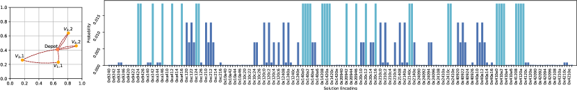
(a) $P1$: $Q\!=\!3$, $V\!=\!\{(0.66,0.41),\{(0.67,0.23),1\},\{(0.81,0.64),2\},\{(0.17,0.26),2\},\{(0.92,0.46),1\}\}$.

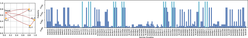
(b) $P2$: $Q\!=\!4$, $V\!=\!\{(0.05,0.68),\{(0.80,0.80),1\},\{(0.97,0.44),3\},\{(0.83,0.25),1\},\{(0.05,0.49),2\}\}$.

Figure 6: Two different problems 6(a) and 6(b), with the optimal solutions (left), and the measured probability distributions of prepared states using depth-$1$ circuits (right). The bars in cyan denote the probabilities of measured optimal encodings. Due to the property of GM-QAOA, the encodings corresponding to the same objective value share the same measured probability.

V Experiments

V-A Experiment Environment and Evaluation Metrics

In the present section, we apply the proposed GM-QAOA solver to address CVRPs. The results are compared to the QAOA, where the cost Hamiltonian is derived from a 1-Phase QUBO formulation [12]. We employ Qiskit’s statevector simulator [29] to perform the quantum circuit simulation, which provides a noise-free probability distribution of measured states when calculating the expected value. Concurrently, the Constrained Optimization BY Linear Approximation (COBYLA) optimizer [30] is adopted to find appropriate parameters for circuits.

Due to the limitation of the simulation environment, we can only construct simple problems. Here, we mainly focus on the convergence of the prepared state, ideally reaching the ground state of the cost Hamiltonian ($H_{C}$). We propose to evaluate the convergence using the optimality gap: computed as,

$$\alpha=\frac{E(\boldsymbol{\gamma},\boldsymbol{\beta})}{C(s^{\ast})}-1,$$ (20)

where $s^{\ast}$ denotes the optimal solution. It signifies the energy difference between the prepared state and the ground state, a lower value of optimality gap corresponds to a more desirable outcome. Furthermore, another metric optimality ratio,

$$r_{opt}=\frac{\text{\# optimal shots}}{\text{\# shots}},$$ (21)

is introduced. The statevector simulator allows the direct computation of $r_{opt}$ as, $\sum_{f^{\ast}}\left\lvert\langle f^{\ast}|\psi(\boldsymbol{\gamma},\boldsymbol{\beta})\rangle\right\rvert^{2}$, where $f^{\ast}$ decodes to the solution with the shortest total distance. This metric indicates the probability of measuring the optimal solution, which directly affects the performance of the solver in real practice. For the results from QAOA, we extend our evaluation to include the feasibility ratio:

$$r_{feas}=\frac{\text{\# feasible shots}}{\text{\# shots}}.$$ (22)

Here, it is calculated as $\sum_{f\in F}\left\lvert\langle f|\psi(\boldsymbol{\gamma},\boldsymbol{\beta})\rangle\right\rvert^{2}$.

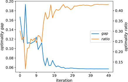
Figure 7: The optimality gap and the optimality ratio of depth-$2$ circuit for $P2$ during the optimization.

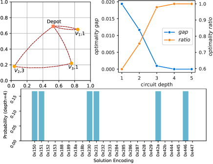
Figure 8: The results of $P3$: $Q\!=\!4$, $V\!\allowbreak=\allowbreak\!\{(\allowbreak 0.53,\allowbreak 0.69),\{(\allowbreak 0.84,\allowbreak 0.65),\allowbreak 1\},\{(\allowbreak 0.04,\allowbreak 0.18),\allowbreak 3\},\{(\allowbreak 0.76,\allowbreak 0.22),\allowbreak 1\}\}$.

V-B Results and Discussion

We begin by building two distinct instances of a $5$-location problem, denoted as $P1$ and $P2$. We simply assume that the vehicle is permitted to travel between any pair of locations with a bidirectional, consistent distance. Notably, the optimal solutions for $P1$ and $P2$, respectively, consist of $3$ and $2$ routes.

We initially solve the problems with the depth-$1$ circuits. Figure 6 shows the measured probability distribution of the optimized circuits for both problem instances. In the case of $P1$, the optimal encodings dominate the distribution, resulting in a significant optimality ratio of $0.597$. Meanwhile, the optimality gap being $0.013$ also indicates that the circuit of $P1$ converges well. However, in $P2$, although the probability of optimal encodings is the highest, the optimality ratio is only $0.241$. This falls below the sum of the secondary peak probabilities. The reason for this due to the discrepancy in the number of encodings associated with the shortest total path in the feasible set. While the number of optimal encodings in $P2$ is $14$, the number of encodings corresponding to the subsequent highest probability is $23$. To improve the results, we apply a depth-$2$ circuit, observing enhanced performance even in the early optimization stage. As illustrated in Figure 7, the optimality surpasses $0.35$ in the middle, ultimately reaching $0.43$.

We investigate further to include deeper circuits on a $4$-location problem instance, $P3$. Figure 8 (top right) shows the optimality gap and optimality ratio of the optimized circuits from depth -$1$ to -$5$. Remarkably, when the depth is set to 4 or 5, the optimized circuits closely approximate the ground state of the cost Hamiltonian, with the optimality gap reaching $1e\!-\!7$ and $1e\!-\!8$, respectively. The probability distribution, as shown in Figure 8 (bottom), is completely dominated by the optimal encodings.

In comparison with the QAOA solver, our proposed method demonstrates an entirely different order of magnitude enhancement across all evaluative metrics, as shown in Table I. Our results are consistent with the conclusions drawn in [9, 12]. It is less reliable to use QAOA for solving constrained combinatorial problems. Meanwhile, as the route number is predefined as $\lceil\sum_{i=1}^{N\!-\!1}q_{i}/Q\rceil$, the search space of QAOA for $P1$ fails to cover the optimal solution.

TABLE I: The evaluation results for the optimized GM-QAOA and QAOA depth-$1$ circuits.

	$P1$		$P2$		$P3$
	GM-QAOA	QAOA	GM-QAOA	QAOA	GM-QAOA	QAOA
optimality gap	$1.27e\!-\!2$	$1.68e\!+\!2$	$1.04e\!-\!1$	$1.60e\!+\!2$	$1.94e\!-\!2$	$1.04e\!+\!2$
feasibility ratio	$1$	$1.77e\!-\!5$	$1$	$1.78e\!-\!5$	$1$	$6.24e\!-\!4$
optimality ratio	$5.97e\!-\!1$	$0$	$2.41e\!-\!1$	$1.30e\!-\!5$	$5.96e\!-\!1$	$1.73e\!-\!4$

Many experiments [31, 32] indicate that the performance of a constant depth circuit deteriorates as the enlarged solution set brings a lower proportion of the optimal encoding, which is also reflected in our results. However, our experiments, albeit limited to simplistic toy examples, show a markedly high optimality ratio. This gives the possibility for our method to solve the problems with an acceptable optimality ratio in practical application. However, further study is required.

VI Conclusion

GM-QAOA offers a general form of mixing operation for preserving the feasibility space, shifting the complexity from mixer design to preparation of the equal amplitude superposition of all feasible states. Initializing from such superpositions has been numerically proven to enhance the solution quality for QAOAs [13]. However, the preparation operation is only applicable to a narrow range of problems. Via reformulation of the problem encoding, this preparation challenge might be mitigated.

In this work, we re-encode the CVRP, allowing quantum states to initialize from an equal amplitude superposition of all feasible states, which also enables the solver to preserve the customer visit constraint via the Grover mixer. Meanwhile, the vehicle capacity constraint is ensured through conditional decoding. Following this, we introduce ancilla conditional indicator bits to derive the cost Hamiltonian. We further demonstrate a method to encode conditions into the ancilla qubits using a polynomial number of basic gates for the phase separation operation. These approaches also carry the potential for extensions to other constrained combinatorial optimization problems, for example, the Knapsack Problems, as they have similar problem structures.

Using statevector simulation, we show the newly designed circuit outperforms the conventional QAOA, exhibiting higher feasibility ratios, higher optimality ratios, and reduced optimality gaps. Notably, these metrics show improvements in the order of magnitude, as supported by the results from three toy examples ($P1$, $P2$, and $P3$).

Despite the advantages of the GM-QAOA framework, our proposed method has several drawbacks. The designed circuit, although with a polynomial number of gates, requires many multi-controlled Toffoli (MCT) gates. The MCT gate is not friendly to topological quantum devices, as it might need additional SWAP gates to adapt to the topology. Also, the bit-flip noises in real quantum devices can easily destroy the feasible space preserved by the Grover Mixer. Thus, it is questionable whether our proposed method is suitable to run on near-term Noisy Intermediate-Scale Quantum (NISQ) [33] devices. Future work must focus on further optimizations and robustness against quantum noise for practical deployment.

References

- [1] G. B. Dantzig and J. H. Ramser, “The truck dispatching problem,” Management science, vol. 6, no. 1, pp. 80–91, 1959.
- [2] L. K. Grover, “A fast quantum mechanical algorithm for database search,” in Proceedings of the twenty-eighth annual ACM symposium on Theory of computing, 1996, pp. 212–219.
- [3] P. W. Shor, “Polynomial-time algorithms for prime factorization and discrete logarithms on a quantum computer,” SIAM review, vol. 41, no. 2, pp. 303–332, 1999.
- [4] A. Montanaro, “Quantum algorithms: an overview,” npj Quantum Information, vol. 2, no. 1, pp. 1–8, 2016.
- [5] E. Farhi, J. Goldstone, and S. Gutmann, “A quantum approximate optimization algorithm,” arXiv preprint arXiv:1411.4028, 2014.
- [6] S. Hadfield, Z. Wang, B. O’gorman, E. G. Rieffel, D. Venturelli, and R. Biswas, “From the quantum approximate optimization algorithm to a quantum alternating operator ansatz,” Algorithms, vol. 12, no. 2, p. 34, 2019.
- [7] G. E. Crooks, “Performance of the quantum approximate optimization algorithm on the maximum cut problem,” arXiv preprint arXiv:1811.08419, 2018.
- [8] C. Moussa, H. Calandra, and V. Dunjko, “To quantum or not to quantum: towards algorithm selection in near-term quantum optimization,” Quantum Science and Technology, vol. 5, no. 4, p. 044009, 2020.
- [9] U. Azad, B. K. Behera, E. A. Ahmed, P. K. Panigrahi, and A. Farouk, “Solving vehicle routing problem using quantum approximate optimization algorithm,” IEEE Transactions on Intelligent Transportation Systems, 2022.
- [10] A. Glos, A. Krawiec, and Z. Zimborás, “Space-efficient binary optimization for variational quantum computing,” npj Quantum Information, vol. 8, no. 1, p. 39, 2022.
- [11] A. Awasthi, F. Bär, J. Doetsch, H. Ehm, M. Erdmann, M. Hess, J. Klepsch, P. A. Limacher, A. Luckow, C. Niedermeier et al., “Quantum computing techniques for multi-knapsack problems,” arXiv preprint arXiv:2301.05750, 2023.
- [12] L. Palackal, B. Poggel, M. Wulff, H. Ehm, J. M. Lorenz, and C. B. Mendl, “Quantum-assisted solution paths for the capacitated vehicle routing problem,” arXiv preprint arXiv:2304.09629, 2023.
- [13] Z. Wang, N. C. Rubin, J. M. Dominy, and E. G. Rieffel, “Xy mixers: Analytical and numerical results for the quantum alternating operator ansatz,” Physical Review A, vol. 101, no. 1, p. 012320, 2020.
- [14] J. Cook, S. Eidenbenz, and A. Bärtschi, “The quantum alternating operator ansatz on max-k vertex cover,” Bulletin of the American Physical Society, vol. 65, 2020.
- [15] A. Bärtschi and S. Eidenbenz, “Grover mixers for qaoa: Shifting complexity from mixer design to state preparation,” in 2020 IEEE International Conference on Quantum Computing and Engineering (QCE). IEEE, 2020, pp. 72–82.
- [16] E. Boros, P. L. Hammer, and G. Tavares, “Local search heuristics for quadratic unconstrained binary optimization (qubo),” Journal of Heuristics, vol. 13, pp. 99–132, 2007.
- [17] A. Mandal, A. Roy, S. Upadhyay, and H. Ushijima-Mwesigwa, “Compressed quadratization of higher order binary optimization problems,” in Proceedings of the 17th ACM International Conference on Computing Frontiers, 2020, pp. 126–131.
- [18] E. Farhi, J. Goldstone, S. Gutmann, and M. Sipser, “Quantum computation by adiabatic evolution,” arXiv preprint quant-ph/0001106, 2000.
- [19] H. Irie, G. Wongpaisarnsin, M. Terabe, A. Miki, and S. Taguchi, “Quantum annealing of vehicle routing problem with time, state and capacity,” 2019.
- [20] S. Feld, C. Roch, T. Gabor, C. Seidel, F. Neukart, I. Galter, W. Mauerer, and C. Linnhoff-Popien, “A hybrid solution method for the capacitated vehicle routing problem using a quantum annealer,” Frontiers in ICT, vol. 6, p. 13, 2019.
- [21] R. Harikrishnakumar, S. Nannapaneni, N. H. Nguyen, J. E. Steck, and E. C. Behrman, “A quantum annealing approach for dynamic multi-depot capacitated vehicle routing problem,” arXiv preprint arXiv:2005.12478, 2020.
- [22] G. Laporte and F. Semet, “Classical heuristics for the capacitated vrp,” in The vehicle routing problem. SIAM, 2002, pp. 109–128.
- [23] K. Shin and S. Han, “A centroid-based heuristic algorithm for the capacitated vehicle routing problem,” Computing and Informatics, vol. 30, no. 4, pp. 721–732, 2011.
- [24] D. de Falco and D. Tamascelli, “An introduction to quantum annealing,” RAIRO-Theoretical Informatics and Applications, vol. 45, no. 1, pp. 99–116, 2011.
- [25] A. Lucas, “Ising formulations of many np problems,” Frontiers in physics, vol. 2, p. 5, 2014.
- [26] Y. Ruan, S. Marsh, X. Xue, Z. Liu, J. Wang et al., “The quantum approximate algorithm for solving traveling salesman problem,” Computers, Materials and Continua, vol. 63, no. 3, pp. 1237–1247, 2020.
- [27] J. T. Seeley, M. J. Richard, and P. J. Love, “The bravyi-kitaev transformation for quantum computation of electronic structure,” The Journal of chemical physics, vol. 137, no. 22, 2012.
- [28] C. Gidney, “Constructing large increment gates,” 2015. [Online]. Available: https://algassert.com/circuits/2015/06/12/Constructing-Large-Increment-Gates.html
- [29] Qiskit contributors, “Qiskit: An open-source framework for quantum computing,” 2023.
- [30] M. J. Powell, A direct search optimization method that models the objective and constraint functions by linear interpolation. Springer, 1994.
- [31] L. Zhou, S.-T. Wang, S. Choi, H. Pichler, and M. D. Lukin, “Quantum approximate optimization algorithm: Performance, mechanism, and implementation on near-term devices,” Physical Review X, vol. 10, no. 2, p. 021067, 2020.
- [32] P. C. Lotshaw, T. S. Humble, R. Herrman, J. Ostrowski, and G. Siopsis, “Empirical performance bounds for quantum approximate optimization,” Quantum Information Processing, vol. 20, no. 12, nov 2021.
- [33] J. Preskill, “Quantum computing in the nisq era and beyond,” Quantum, vol. 2, p. 79, 2018.