Amplifying Frequency Up-Converted Infrared Signals with a Molecular Optomechanical Cavity

Abstract

Frequency up-conversion, enabled by molecular optomechanical coupling, has recently emerged as a promising approach for converting infrared signals into the visible range through quantum coherent conversion of signals. However, detecting these converted signals poses a significant challenge due to their inherently weak signal intensity. In this work, we propose an amplification mechanism capable of enhancing the signal intensity by a factor of 1000 or more in a molecular-cavity system consisting $10^{7}$ molecules. The mechanism takes advantage of the strong coupling enhancement with molecular collective mode and Stokes sideband pump. Our work demonstrates a feasible approach for up-converting infrared signals to the visible range.

Introduction—The mid- and far-infrared frequency range, encompassing wavelengths from 2.5 to 500 $\mu\text{m}$, is a critical region of the electromagnetic spectrum with significant applications in many fields, including thermal imaging [1], quantum sensing [2], microscopy [3, 4], clinical medicine [5], and astronomical surveys [6, 7]. However, detecting photons within this range presents a significant challenge, as conventional infrared detectors are sensitive to the thermal noise at the frequency vicinity of these photons, and require cryogenic temperatures to reduce this noise. As a result, there is a pressing need for detection technologies that can operate within this frequency range without the need for cryogenic cooling.

One promising approach is to utilize coherent up-conversion technology [8, 9, 10, 11, 12, 13, 14] to convert lower-frequency infrared (IR) light into the visible or near-infrared (VIS/NIR) range, which can be detected using cost-effective and highly sensitive VIS/NIR cameras. This strategy takes advantage of the well-developed infrastructure and capabilities of VIS/NIR cameras, including their high integration and low cost, making it an attractive option for a wide range of applications. Recently, molecular optomechanical cavities have emerged as a promising candidate to realize coherent frequency up-conversion [15]. In the optical cavities, the molecular vibrational motion is bilinearly coupled to the IR field and optomechanically coupled to the VIS field to be converted into. The advantages to couple multiple molecules and enhance coupling strength via cavity result in a great enhancement of the detection efficiency [16, 17] beyond the conventional optomechanical cavity setup [18, 19, 20, 21, 22, 23, 24, 25, 26, 27, 28, 29, 30, 31]. The question still remains as to whether this system is capable of detecting a weak infrared (IR) signal at the several-photon level with enhanced sensitivity.

In this Letter, we propose a scheme to amplify the signal intensity of the up-converted VIS photons in the molecular optomechanical cavity system with a blue-tuned pump field, tuned close to the first Stokes sideband frequency of VIS mode. We show that the factor of 1000 (or more) of amplification can be achieved. Our work shall provide a new perspective to reveal the potentials of the molecular optomechanical cavity.

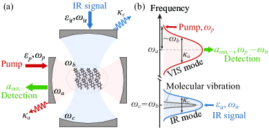
Figure 1: (a) The molecular optomechanical cavity consisting of $N$ molecules (with frequency $\omega_{b}$ of the vibrational mode) coupled to both the VIS mode (with frequency $\omega_{a}$ and decay rate $\kappa_{a}$) via the optomechanical interaction and the IR mode (with frequency $\omega_{c}$ and decay rate $\kappa_{c}$) via the bilinear interaction. The VIS mode is driven by a pump field with frequency $\omega_{p}$ and amplitude $\varepsilon_{p}$. The IR signal of interest with frequency $\omega_{\mathrm{ir}}$ and amplitude $\varepsilon_{\mathrm{ir}}$ is incident on the cavity with coupling to the IR mode $c$. (b) Scheme of frequency up-convered IR signals based on the molecular optomechanical cavity. Here the IR signal of interest is near-resonant with the vibrational frequency of the molecules (as well as the IR mode $c$) and the blue-detuned pump field is near-resonant with the first Stokes sideband of the VIS mode, i.e., $\omega_{\mathrm{ir}}\simeq\omega_{b}=\omega_{c}$ and $\omega_{p}\simeq\omega_{a}+\omega_{b}$. The input weak IR signal with amplitude $\varepsilon_{\mathrm{ir}}$ and frequency $\omega_{\mathrm{ir}}$ is up-converted as the output VIS signal ($a_{\text{out},-}$) with frequency $\omega_{p}-\omega_{\mathrm{ir}}$ via the optomechanical interaction between the VIS mode and the molecular vibration.

Model.—The molecular optomechanical cavity consists of $N$ molecules and a cavity supporting both VIS and IR modes, as shown in Fig. 1(a). The cavity can be nanoparticles [16, 17], supporting two plasmonic modes with frequencies $\omega_{a}$ at the VIS region with annihilation operator $a$ and $\omega_{c}$ at the IR region with annihilation operator $c$. Molecules are specifically chosen to couple with both the VIS and IR modes [15, 16, 17]. A strong pump field at the visible range with frequency $\omega_{p}$ and amplitude $\varepsilon_{p}$ is applied to drive the VIS mode $a$ in the cavity. The weak IR signal of interest with frequency $\omega_{\mathrm{ir}}$ and amplitude $\varepsilon_{\mathrm{ir}}$ is incident on the cavity and couples to the IR mode $c$. In the interaction picture with respect to $H_{0}=\hbar\omega_{p}a^{\dagger}a$, the Hamiltonian of the system is given as ($\hbar=1$)

$$H_{\text{sys}} =\Delta_{0}a^{\dagger}a+\omega_{c}c^{\dagger}c+\sum_{j=1}^{N}\omega_{b}b_{j}^{\dagger}b_{j}$$

$$\quad+\sum_{j=1}^{N}g_{a}a^{\dagger}a(b_{j}^{\dagger}+b_{j})+\sum_{j=1}^{N}g_{c}(c^{\dagger}+c)(b_{j}^{\dagger}+b_{j})$$

$$\quad+i(\varepsilon_{p}a^{\dagger}+\varepsilon_{\mathrm{ir}}e^{-i\omega_{\mathrm{ir}}t}c^{\dagger}-\text{H.c.}),$$ (1)

where $b_{j}$ ($b_{j}^{\dagger}$) is the annihilation (creation) operator of the vibrational mode of the $j$th molecule with resonance frequency $\omega_{b}$. The fourth term describes the optomechanical interaction between the VIS mode and the molecular vibration with the coupling strength $g_{a}$ and the fifth term represents the bilinear interaction between the IR mode and the molecular vibration with the coupling strength $g_{c}$. The term including $\varepsilon_{p}$ ($\varepsilon_{\mathrm{ir}}$) describes the driving pump field to the VIS mode (the coupling of the detected IR signal to the IR mode). The parameter $\Delta_{0}=\omega_{a}-\omega_{p}$ is the detuning of the VIS mode with respect to the pump driving. Without loss of generality, we assume these parameters ($g_{a}$, $g_{c}$, $\varepsilon_{p}$, and $\varepsilon_{\mathrm{ir}}$) are real numbers.

In the cases of large number of the molecules $N\gg 1$ and the low-excitation limit of the molecular vibration, by introducing the molecular collective operator $B=\sum_{j=1}^{N}b_{j}/\sqrt{N}$ satisfying approximately $[B,B^{\dagger}]=1$ [32, 33, 34], Hamiltonian in Eq. (1) is simplified as

$$H =\Delta_{0}a^{\dagger}a+\omega_{c}c^{\dagger}c+\omega_{b}B^{\dagger}B+G_{c}(c^{\dagger}+c)(B^{\dagger}+B)$$

$$+G_{a}a^{\dagger}a(B^{\dagger}+B)+i(\varepsilon_{p}a^{\dagger}+\varepsilon_{\mathrm{ir}}e^{-i\omega_{\mathrm{ir}}t}c^{\dagger}-\text{H.c.}),$$ (2)

where $G_{a}=g_{a}\sqrt{N}$ ($G_{c}=g_{c}\sqrt{N}$) is the collective optomechanical (bilinear) coupling strength. The quantum Langevin equations (QLEs) for the cavity modes $a$ and $c$ and the molecular collective mode $B$ are obtained as

$$\dot{a} =-(i\Delta_{0}+\kappa_{a})a-iG_{a}a(B^{\dagger}+B)+\varepsilon_{p}+\sqrt{2\kappa_{a}}a_{\text{in}},$$ (3a)

$$\dot{c} =-(i\omega_{c}+\kappa_{c})c-iG_{c}(B^{\dagger}+B)+\varepsilon_{\mathrm{ir}}e^{-i\omega_{\mathrm{ir}}t}+\sqrt{2\kappa_{c}}c_{\text{in}},$$ (3b)

$$\dot{B} =-(i\omega_{b}+\gamma_{B})B-iG_{a}a^{\dagger}a-iG_{c}(c^{\dagger}+c)+\sqrt{2\gamma_{B}}B_{\text{in}},$$ (3c)

where $\kappa_{a}$ ($\kappa_{c}$) and $\gamma_{B}$ are the decay rates of the VIS (IR) mode and the molecular collective mode, respectively. $a_{\text{in}}$, $c_{\text{in}}$, and $B_{\text{in}}$ are the noise operators with zero mean values $\langle o_{\text{in}}\rangle=0$ for $o=a,c,B$. And the amplitude of the IR signal $\varepsilon_{\mathrm{ir}}$ of interest is much smaller than that of the pump field $\varepsilon_{p}$, and thus treated as the perturbation. The relations between steady-state mean values of the operators $o=a,c,B$ are obtained by neglecting the $\varepsilon_{\mathrm{ir}}\exp(-i\omega_{\mathrm{ir}}t)$ term in Eq. (3b) as $\langle c\rangle_{\text{ss}}=-iG_{c}(\langle B\rangle_{\text{ss}}+\langle B\rangle_{\text{ss}}^{*})/(i\omega_{c}+\kappa_{c})$, $\langle B\rangle_{\text{ss}}=-i[G_{a}|\langle a\rangle_{\text{ss}}|^{2}+G_{c}(\langle c\rangle_{\text{ss}}+\langle c\rangle_{\text{ss}}^{*})]/(i\omega_{b}+\gamma_{B})$, and $\langle a\rangle_{\text{ss}}=\varepsilon_{p}/(i\Delta+\kappa_{a})$. Here $\Delta=\Delta_{0}+G_{a}(\langle B\rangle_{\text{ss}}^{*}+\langle B\rangle_{\text{ss}})$ is the effective detuning caused by the collective optomechanical interaction. These steady-state mean values are solved self-consistently.

The up-converted IR signal is analyzed via the quantum fluctuation $\delta o=o-\langle o\rangle_{\text{ss}}$ ($o=a,c,B$) on the top of the steady-state value [35]. Keeping terms up to the first order of quantum fluctuation, we obtain the linearized QLEs as

$$\delta\dot{a} =-(i\Delta+\kappa_{a})\delta a-i\mathcal{G}_{a}(\delta B^{\dagger}+\delta B)+\sqrt{2\kappa_{a}}a_{\text{in}},$$

$$\delta\dot{c} =-(i\omega_{c}+\kappa_{c})\delta c-iG_{c}(\delta B^{\dagger}+\delta B)+\varepsilon_{\mathrm{ir}}e^{-i\omega_{\mathrm{ir}}t}$$

$$\quad+\sqrt{2\kappa_{c}}c_{\text{in}},$$

$$\delta\dot{B} =-(i\omega_{b}+\gamma_{B})\delta B-i(\mathcal{G}_{a}^{*}\delta a+\mathcal{G}_{a}\delta a^{\dagger})$$

$$\quad-iG_{c}(\delta c+\delta c^{\dagger})+\sqrt{2\gamma_{B}}B_{\text{in}},$$ (4)

where $\mathcal{G}_{a}=G_{a}\langle a\rangle_{\text{ss}}$ is the enhanced collective optomechanical coupling strength by the strong pump field. Note that the $\varepsilon_{\mathrm{ir}}\exp(-i\omega_{\mathrm{ir}}t)$ term is now included in Eq. (4). Here we have not used the rotating-wave approximation (RWA) to both the optomechanical interaction and the bilinear interaction terms.

To solve the linearized QLEs (4), we use the ansatz $\langle\delta o\rangle=o_{+}e^{-i\omega_{\mathrm{ir}}t}+o_{-}e^{i\omega_{\mathrm{ir}}t}$ for $o=a,c,B$ [36, 35, 37, 38], where $o_{+}$ and $o_{-}$ correspond to the values of positive- and negative-frequency components, respectively. With this ansatz, $o_{\pm}$ and $o_{\pm}^{*}$ are solved analytically. And the detailed discussion is presented in the Supplementary Material [39].

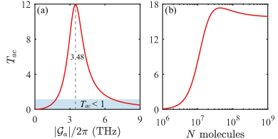
Figure 2: (a) The conversion efficiency $T_{ac}$ as a function of the enhanced collective optomechanical coupling strength $|\mathcal{G}_{a}|$ for $N=10^{7}$. (b) The conversion efficiency $T_{ac}$ as a function of the number of the molecules $N$ at $g_{a}/2\pi=0.08\,\text{GHz}$. Here we consider the resonance case $\omega_{\mathrm{ir}}=\omega_{b}=\omega_{c}=2\pi\times 30\,\text{THz}$ and other parameters are $\Delta=-\omega_{b}$, $\kappa_{a}/2\pi=30\,\text{THz}$, $\kappa_{c}/2\pi=0.5\,\text{THz}$, $\gamma_{B}/2\pi=0.16\,\text{THz}$, $\varepsilon_{p}/2\pi=500\,\text{THz}$, and $g_{c}/2\pi=0.1\,\text{GHz}$.

Amplification.—The IR signal of interest is amplified when the frequency of the pump field is tuned close to the first Stokes sideband of the VIS mode, i.e., $\Delta=-\omega_{b}$. The amplified up-convered signal is included in the quantum fluctuation $\delta a$ of the VIS mode. The detection is performed on the output field of the VIS mode $a_{\text{out}}=\langle a_{\text{out}}\rangle_{\text{ss}}+\delta a_{\text{out}}$, where $\langle a_{\text{out}}\rangle_{\text{ss}}$ ($\delta a_{\text{out}}$) denotes the steady-state (fluctuation) component of the output field $a_{\text{out}}$. The mean value of the fluctuation component is rewritten as $\langle\delta a_{\text{out}}\rangle=a_{\text{out},+}e^{-i\omega_{\mathrm{ir}}t}+a_{\text{out},-}e^{i\omega_{\mathrm{ir}}t}$, where $a_{\text{out},+}$ and $a_{\text{out},-}$ are the first anti-Stokes and Stokes components of $\langle\delta a_{\text{out}}\rangle$, respectively. With the input-output relation $a_{\text{out}}+a_{\text{in}}+\varepsilon_{p}/\sqrt{2\kappa_{a}}=\sqrt{2\kappa_{a}}a$ [40], we obtain output signal as $a_{\text{out},\pm}=\sqrt{2\kappa_{a}}a_{\pm}$.

At the case of the blue-detuned pump field ($\Delta=-\omega_{b}$), we mainly concern about the upconversion at the first Stokes sideband. For the near-resonant case $\omega_{\mathrm{ir}}\simeq\omega_{b}=\omega_{c}$, the first Stokes component $a_{-}$ is obtained explicitly as [39]

$$a_{-}=\frac{2i\varepsilon_{\mathrm{ir}}\mathcal{G}_{a}G_{c}\Delta(\Delta-\omega_{\text{ir}}+i\kappa_{a})(\Delta-\omega_{\text{ir}}+i\kappa_{c})}{\mathcal{A}(\omega_{\text{ir}})},$$ (5)

where $\mathcal{A}(\omega_{\text{ir}})=\{[\Delta^{2}-(\omega_{\text{ir}}-i\kappa_{c})^{2}][\Delta^{2}-(\omega_{\text{ir}}-i\gamma_{B})^{2}]-4G_{c}^{2}\Delta^{2}\}[\Delta^{2}-(\omega_{\text{ir}}-i\kappa_{a})^{2}]+4|\mathcal{G}_{a}|^{2}\Delta^{2}[\Delta^{2}-(\omega_{\text{ir}}-i\kappa_{c})^{2}]$. For the input IR signal $\varepsilon_{\mathrm{ir}}/\sqrt{2\kappa_{c}}$ [39], the conversion efficiency $T_{ac}$ at the first Stokes sideband is obtained as

$$T_{ac}=|t_{ac}|^{2}=\left|\frac{2\sqrt{\kappa_{a}\kappa_{c}}a_{-}}{\varepsilon_{\mathrm{ir}}}\right|^{2},$$ (6)

where $t_{ac}\equiv a_{\text{out},-}/\left(\varepsilon_{\mathrm{ir}}/\sqrt{2\kappa_{c}}\right)$ denotes the conversion coefficient from IR signal to VIS range at the first Stokes sideband [41, 38].

For simplicity, we first consider the case in which the IR signal is fully resonant with the vibrational frequency of the molecules (as well as the IR mode), i.e., $\omega_{\mathrm{ir}}=\omega_{b}=\omega_{c}$. In this case, the conversion coefficient is explicitly as $t_{ac}=2\sqrt{\kappa_{a}\kappa_{c}}\mathcal{G}_{a}G_{c}/(G_{c}^{2}\kappa_{a}\eta_{c}^{-1}-|\mathcal{G}_{a}|^{2}\kappa_{c}\eta_{a}^{-1}+\kappa_{a}\kappa_{c}\gamma_{B}\eta_{B})$, where $\eta_{a,c}=1+i\kappa_{a,c}/(2\Delta)$ and $\eta_{B}=1+i\gamma_{B}/(2\Delta)$ [39].

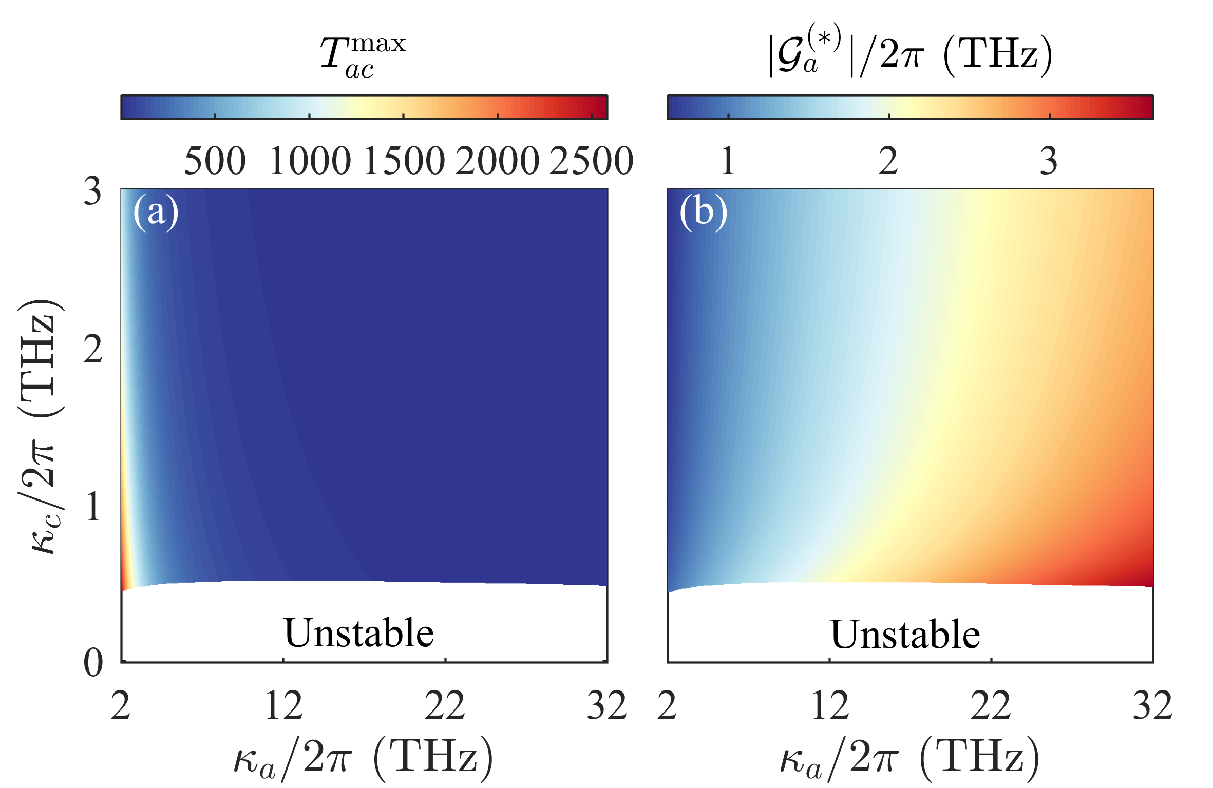
Figure 3: (a) The maximum conversion efficiency $T_{ac}$ as functions of the decay rates $\kappa_{a}$ and $\kappa_{c}$ at optimal coupling strength $|\mathcal{G}_{a}^{(*)}|\simeq\sqrt{(G_{c}^{2}|\eta_{c}^{-1}|+\kappa_{c}\gamma_{B}|\eta_{B}|)\kappa_{a}|\eta_{a}|/\kappa_{c}}$. (b) The optimal coupling strength $|\mathcal{G}_{a}^{(*)}|$ as functions of the decay rates $\kappa_{a}$ and $\kappa_{c}$. Here $N=10^{7}$ and other parameters are the same as those in Fig. 2.

Figure 2(a) shows the conversion efficiency $T_{ac}$ as a function of the enhanced collective optomechanical coupling strength $|\mathcal{G}_{a}|$ at the first Stokes sideband $\Delta=-\omega_{b}$. In the numerical simulations, we choose the experimentally feasible parameters [42, 43, 16, 17, 44, 45, 46, 47, 48, 49, 50]: $\omega_{\mathrm{ir}}/2\pi=\omega_{b}/2\pi=\omega_{c}/2\pi=30\,\text{THz}$, $\kappa_{a}/2\pi=30\,\text{THz}$, $\kappa_{c}/2\pi=0.5\,\text{THz}$, $\gamma_{B}/2\pi=0.16\,\text{THz}$, $\varepsilon_{p}/2\pi=500\,\text{THz}$, $g_{c}/2\pi=0.1\,\text{GHz}$, and $N=10^{7}$. One scheme for realizing the molecular-cavity system is that an Au nanoparticle inside a nanogroove is etched in a gold film to form the cavity. Biphenyl-4-thiol molecules are chosen to support a prominent vibrational mode that is coupled to both the VIS and IR modes of the cavity [16]. And the single-photon optomechanical coupling strength between the VIS mode and the molecular vibration reaches $g_{a}\sim 2\pi\times 100\,\text{GHz}$ [45]. For other molecule (e.g. rhodamine 6G molecule), the single-photon optomechanical coupling strength $g_{a}$ is at the range $2\pi\times\left(0.006-145\right)\,\text{MHz}$ [46].

The curve in Fig. 2(a) shows that $T_{ac}$ is larger than unity under the appropriate coupling strength condition to achieve the amplification of frequency up-converted IR signal. In addition, we observe that the conversion efficiency of the IR signal reaches a maximum (i.e., $T_{ac}^{\mathrm{max}}\approx 12$) at optimal coupling strength [39] $|\mathcal{G}_{a}|=|\mathcal{G}_{a}^{(*)}|\simeq\sqrt{(G_{c}^{2}|\eta_{c}^{-1}|+\kappa_{c}\gamma_{B}|\eta_{B}|)\kappa_{a}|\eta_{a}|/\kappa_{c}}=2\pi\times 3.48\,\text{THz}$ for the given parameters. In Fig. 2(b), we illustrates the dependence of the conversion efficiency $T_{ac}$ of the IR signal on the number of molecules. The curve shows a non-monotonic behavior with an optimal number of molecules around $10^{7}$ to reach highest conversion efficiency. The curve also shows a plateau where the conversion efficiency stays constant with increasing the number of molecules.

Other key parameters that determine the conversion efficiency of the IR signal are the decay rates $\kappa_{c}$ and $\kappa_{a}$ of the IR and VIS modes. In Fig. 3(a), we plot the maximum conversion efficiency $T_{ac}^{\mathrm{max}}$ at first Stokes sideband as functions of the decay rates $\kappa_{a}$ and $\kappa_{c}$ at optimal coupling strength $|\mathcal{G}_{a}^{(*)}|$. Figure 3(a) shows that for fixed the decay rate $\kappa_{c}$ (e.g. $\kappa_{c}/2\pi=1\,\text{THz}$), $T_{ac}^{\mathrm{max}}$ is significantly improved by decreasing the decay rate $\kappa_{a}$ of the cavity VIS mode. However, when the decay rate is fixed (e.g. $\kappa_{a}/2\pi=30\,\text{THz}$), $T_{ac}^{\mathrm{max}}$ increases slowly with the increase of the decay rate $\kappa_{c}$ of the cavity IR mode. In particular, the conversion efficiency $T_{ac}$ with a factor around 1000 is achieved at $\kappa_{a}/2\pi=2\,\text{THz}$. These results highlight the importance of controlling the decay rates of the IR and VIS modes for amplifying frequency up-converted IR signal. Figure 3(b) shows the optimal coupling strength $|\mathcal{G}_{a}^{(*)}|$ as functions of the decay rates $\kappa_{a}$ and $\kappa_{c}$. The results show that the optimal coupling strength $|\mathcal{G}_{a}^{(*)}|$ increases (decreases) as the value of $\kappa_{a}$ ($\kappa_{c}$) increases.

The molecular optomechanical system could become unstable once the optomechanical and bilinear coupling strengths are strong enough [51]. We check the stability of the system with amplification and mark the unstable region in Fig. 3. The stability condition of the system is given explicitly according to the Routh-Hurwitz criterion [52, 53]. Mathematically, the system is stable only if the real parts of all the eigenvalues of the coefficient matrix [see Eq. (S10) in the Supplementary Materials] are positive. Physically, the negative real part of the eigenvalue of this coefficient matrix represents the gain for the related diagonalized normal mode causing the instability. The detailed discussion of the stability is presented in the Supplementary Material [39].

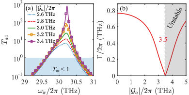
Figure 4: (a) The conversion efficiency $T_{ac}$ as a function of the frequency of the IR signal $\omega_{\text{ir}}$ for different values of $|\mathcal{G}_{a}|$. (b) The bandwidth $\Gamma$ as a function of the enhanced collective optomechanical coupling strength $|\mathcal{G}_{a}|$. Here $N=10^{7}$ and other parameters are the same as those in Fig. 2. In panel (b), the unstable region is marked with the grey shadow.

Bandwidth of the amplification.—Another key characteristic of the up-conversion is the bandwidth of the detection. In the following we explore the dependence of the conversion efficiency on the frequency of the IR signal of interest. For the near-resonant incident IR signal $\omega_{\text{ir}}\simeq\omega_{b}=\omega_{c}$, the conversion efficiency of the IR signal to the VIS range at the first Stokes sideband is obtained as $T_{ac}=|4\sqrt{\kappa_{a}\kappa_{c}}\mathcal{G}_{a}G_{c}\Delta(\Delta-\omega_{\text{ir}}+i\kappa_{a})(\Delta-\omega_{\text{ir}}+i\kappa_{c})/\mathcal{A}(\omega_{\text{ir}})|^{2}$. Figure 4(a) shows the dependence of the conversion efficiency $T_{ac}$ as a function of the frequency $\omega_{\mathrm{ir}}$ of the IR signal for different coupling strength $\mathcal{G}_{a}$. As the enhanced collective optomechanical coupling strength $|\mathcal{G}_{a}|$ increases, the maximum conversion efficiency of the IR signal increases. For the resonance case $\omega_{\text{ir}}=\omega_{b}=\omega_{c}$, the maximum conversion efficiency ($T_{ac}^{\mathrm{max}}\approx 12$) is obtained at $|\mathcal{G}_{a}|/2\pi\approx 3.48\,\text{THz}$, as shown in Fig. 2(a). However, for the near-resonant incident IR signal $\omega_{\text{ir}}\simeq\omega_{b}=\omega_{c}$, we find higher amplification than the resonance case for frequency up-conversion. For example, the maximum conversion efficiency $T_{ac}^{\mathrm{max}}$ of the IR signal is approximately $750$ at $|\mathcal{G}_{a}|/2\pi=3.4\,\text{THz}$, and the range of the amplification for IR signal is as $29.6\,\text{THz}\lesssim\omega_{\text{ir}}/2\pi\lesssim 30.6\,\text{THz}$.

The bandwidth $\Gamma$ of the conversion efficiency is obtained by estimating the full width $\Gamma$ at half maximum [51, 54]. In Fig. 4(b), we illustrate the bandwidth $\Gamma$ as a function of the enhanced collective optomechanical coupling strenght $|\mathcal{G}_{a}|$ with the unstable region marked with the gray shadow. The bandwidth $\Gamma$ decreases with the increase of $|\mathcal{G}_{a}|$ in the stable region. At $|\mathcal{G}_{a}|/2\pi\approx 3.5\,\text{THz}$, we observe that the bandwidth is $\Gamma\approx 0$ for the near-resonant case $\omega_{\text{ir}}\simeq\omega_{b}=\omega_{c}$, where the conversion efficiency of the IR signal diverges. The current figure illustrates a trade off between the conversion efficiency and the bandwidth for choosing the proper coupling strength $|\mathcal{G}_{a}|$. We also present the equivalent analyses of the conversion efficiency and the bandwidth with the power spectrum method [55, 54] in the Supplementary Material [39] to confirm the current results.

Conclusion.—We have proposed an amplification scheme to increase the sensitivity of the detecting IR signal in the molecular optomechanical cavity, where the IR signal is up-converted into the photons at the visible range. In our scheme, the IR signal of interest is resonant (or near-resonant) with the molecular vibration, and the blue-detuned pump field, which is near-resonant with the first Stokes sideband of the VIS mode, is utilized to pump the cavity mode . We find out the amplification with the factor of several thousands at the first Stokes sideband of the VIS mode with designed parameters of the cavity and the molecules and verify the existence of the stability of scheme. Our scheme shall provide insight into the design efficient up-conversion detection of IR signal to achieve the detection on the signal photon level.

This work is supported by the National Natural Science Foundation of China (Grants No. 12074030, No. 12088101, No. 11875049, No. 12274107, and No. U2230402) and the China Postdoctoral Science Foundation (Grant No. 2021M700360).

Fen Zou,^1,2 Lei Du,³ Yong Li,^1,∗ and Hui Dong^4,†

¹Center for Theoretical Physics, Hainan University, Haikou 570228, China
²Beijing Computational Science Research Center, Beijing 100193, China
³Center for Quantum Sciences and School of Physics, Northeast Normal University, Changchun 130024, China
⁴Graduate School of China Academy of Engineering Physics, Beijing 100193, China

The current Supplementary Material provides detailed derivations of the results in the main text, and supporting discussions. In Sec. S1, we provide details on the calculation of the values of the positive- and negative-frequency components $o_{\pm}$ based on the response to the input IR signal. In addition, using such an optical response method, we present the analytical expression of the conversion efficiency from IR signal to VIS range at the first Stokes sideband for the blue-detuned pump field. In Sec. S2, we provide an alternative power spectrum method to calculate the conversion efficiency from IR signal to VIS range in the frequency domain. In Sec. S3, we give a detailed discussion on the stability of the system.

S1 detailed calculation of the values of the positive- and negative-frequency components $o_{\pm}$ and the conversion efficiency of the ir signal

We assume that the amplitude of the IR signal of interest $\varepsilon_{\text{ir}}$ is much smaller than that of the pump field $\varepsilon_{p}$, and then the steady-state mean values of the operators $o$ will not be affected by the IR signal. Hence, in the absence of the $\varepsilon_{\text{ir}}\exp(-i\omega_{\text{ir}}t)$ term in Eq. (3) in the main text, the equations of motion for the steady-state mean values of the operators are obtained as

$$0 =-(i\Delta_{0}+\kappa_{a})\langle a\rangle_{\text{ss}}-iG_{a}\langle a\rangle_{\text{ss}}(\langle B\rangle_{\text{ss}}^{*}+\langle B\rangle_{\text{ss}})+\varepsilon_{p},$$

$$0 =-(i\omega_{c}+\kappa_{c})\langle c\rangle_{\text{ss}}-iG_{c}(\langle B\rangle_{\text{ss}}^{*}+\langle B\rangle_{\text{ss}}),$$ (S1)

$$0 =-(i\omega_{b}+\gamma_{B})\langle B\rangle_{\text{ss}}-iG_{a}\langle a\rangle_{\text{ss}}^{*}\langle a\rangle_{\text{ss}}-iG_{c}(\langle c\rangle_{\text{ss}}^{*}+\langle c\rangle_{\text{ss}}),$$

where we have used a mean-field like approximation $\langle a^{\dagger}a\rangle_{\text{ss}}\equiv\langle a^{\dagger}\rangle_{\text{ss}}\langle a\rangle_{\text{ss}}$. This is reasonable when the mean photon number is much larger than 1 (i.e., $\langle a^{\dagger}a\rangle_{\text{ss}}\gg 1$). The steady-state mean values of the operators are obtained by solving Eq. (S1) as

$$\langle a\rangle_{\text{ss}}=\frac{\varepsilon_{p}}{i\Delta+\kappa_{a}},\quad\langle c\rangle_{\text{ss}}=-\frac{iG_{c}(\langle B\rangle_{\text{ss}}^{*}+\langle B\rangle_{\text{ss}})}{i\omega_{c}+\kappa_{c}},\quad\langle B\rangle_{\text{ss}}=-\frac{i[G_{a}|\langle a\rangle_{\text{ss}}|^{2}+G_{c}(\langle c\rangle_{\text{ss}}^{*}+\langle c\rangle_{\text{ss}})]}{i\omega_{b}+\gamma_{B}},$$ (S2)

where $\Delta=\Delta_{0}+G_{a}(\langle B\rangle_{\text{ss}}^{*}+\langle B\rangle_{\text{ss}})$ is the effective detuning including the frequency shift caused by the collective optomechanical interaction.

Under the condition of the strong pump field, each operator is expanded as the sum of its steady-state mean value and quantum fluctuation operator, i.e., $o=\langle o\rangle_{\text{ss}}+\delta o$ for $o=a,c,B$. When the weak IR signal is present, it can be taken as the perturbation, and the mean value of the fluctuation operator is not zero.

In the presence of the weak IR signal, to solve the mean value of the fluctuation operator, we use the ansatz $\langle\delta o\rangle=o_{+}e^{-i\omega_{\text{ir}}t}+o_{-}e^{i\omega_{\text{ir}}t}$ for $o=a,c,B$, where $o_{+}$ and $o_{-}$ describe the values of positive- and negative-frequency components, respectively, originated from the response to the input IR signal due to the optomechanical and bilinear couplings. Note that $a_{+}$ and $a_{-}$ are, respectively, the first anti-Stokes and Stokes components of $\langle\delta a\rangle$ [1, 2, 3]. By substituting them into Eq. (4) in the main text, the equations of motion for $o_{\pm}$ are obtained as

$$-i\omega_{\text{ir}}a_{+} =-(i\Delta+\kappa_{a})a_{+}-i\mathcal{G}_{a}(B_{+}+B_{-}^{*}),$$

$$i\omega_{\text{ir}}a_{-} =-(i\Delta+\kappa_{a})a_{-}-i\mathcal{G}_{a}(B_{-}+B_{+}^{*}),$$

$$-i\omega_{\text{ir}}c_{+} =-(i\omega_{c}+\kappa_{c})c_{+}-iG_{c}(B_{+}+B_{-}^{*})+\varepsilon_{\text{ir}},$$ (S3)

$$i\omega_{\text{ir}}c_{-} =-(i\omega_{c}+\kappa_{c})c_{-}-iG_{c}(B_{-}+B_{+}^{*}),$$

$$-i\omega_{\text{ir}}B_{+} =-(i\omega_{b}+\gamma_{B})B_{+}-i(\mathcal{G}_{a}^{*}a_{+}+\mathcal{G}_{a}a_{-}^{*})-iG_{c}(c_{+}+c_{-}^{*}),$$

$$i\omega_{\text{ir}}B_{-} =-(i\omega_{b}+\gamma_{B})B_{-}-i(\mathcal{G}_{a}^{*}a_{-}+\mathcal{G}_{a}a_{+}^{*})-iG_{c}(c_{-}+c_{+}^{*}),$$

and the equations of motion for $o_{\pm}^{*}$ are obtained as

$$i\omega_{\text{ir}}a_{+}^{*} =-(-i\Delta+\kappa_{a})a_{+}^{*}+i\mathcal{G}_{a}^{*}(B_{+}^{*}+B_{-}),$$

$$-i\omega_{\text{ir}}a_{-}^{*} =-(-i\Delta+\kappa_{a})a_{-}^{*}+i\mathcal{G}_{a}^{*}(B_{-}^{*}+B_{+}),$$

$$i\omega_{\text{ir}}c_{+}^{*} =-(-i\omega_{c}+\kappa_{c})c_{+}^{*}+iG_{c}(B_{+}^{*}+B_{-})+\varepsilon_{\text{ir}},$$ (S4)

$$-i\omega_{\text{ir}}c_{-}^{*} =-(-i\omega_{c}+\kappa_{c})c_{-}^{*}+iG_{c}(B_{-}^{*}+B_{+}),$$

$$i\omega_{\text{ir}}B_{+}^{*} =-(-i\omega_{b}+\gamma_{B})B_{+}^{*}+i(\mathcal{G}_{a}a_{+}^{*}+\mathcal{G}_{a}^{*}a_{-})+iG_{c}(c_{+}^{*}+c_{-}),$$

$$-i\omega_{\text{ir}}B_{-}^{*} =-(-i\omega_{b}+\gamma_{B})B_{-}^{*}+i(\mathcal{G}_{a}a_{-}^{*}+\mathcal{G}_{a}^{*}a_{+})+iG_{c}(c_{-}^{*}+c_{+}).$$

In the resonant case $\omega_{\text{ir}}=\omega_{b}=\omega_{c}$ and the blue-detuned pump field $\Delta=-\omega_{b}$, the values of positive- and negative-frequency components $o_{\pm}$ are obtained by solving Eqs. (S3) and (S4) as

$$a_{+} =\frac{2i\Delta\mathcal{G}_{a}G_{c}\kappa_{a}(2\Delta-i\kappa_{c})\varepsilon_{\text{ir}}}{4G_{c}^{2}\Delta^{2}\kappa_{a}(2\Delta-i\kappa_{a})-[4|\mathcal{G}_{a}|^{2}\Delta^{2}-\kappa_{a}\gamma_{B}(2\Delta-i\gamma_{B})(2\Delta-i\kappa_{a})](2\Delta-i\kappa_{c})\kappa_{c}},$$

$$a_{-} =\frac{2\Delta\mathcal{G}_{a}G_{c}(2\Delta+i\kappa_{a})(2\Delta+i\kappa_{c})\varepsilon_{\text{ir}}}{4G_{c}^{2}\Delta^{2}\kappa_{a}(2\Delta+i\kappa_{a})-[4|\mathcal{G}_{a}|^{2}\Delta^{2}-\kappa_{a}\gamma_{B}(2\Delta+i\gamma_{B})(2\Delta+i\kappa_{a})](2\Delta+i\kappa_{c})\kappa_{c}},$$

$$c_{+} =\frac{\{(2\Delta-i\kappa_{a})\kappa_{a}[\gamma_{B}(2\Delta-i\gamma_{B})(2\Delta-i\kappa_{c})+2iG_{c}^{2}\Delta]-4|\mathcal{G}_{a}|^{2}\Delta^{2}(2\Delta-i\kappa_{c})\}\varepsilon_{\text{ir}}}{4G_{c}^{2}\Delta^{2}\kappa_{a}(2\Delta-i\kappa_{a})-[4|\mathcal{G}_{a}|^{2}\Delta^{2}-\kappa_{a}\gamma_{B}(2\Delta-i\gamma_{B})(2\Delta-i\kappa_{a})](2\Delta-i\kappa_{c})\kappa_{c}},$$

$$c_{-} =\frac{2i\Delta G_{c}^{2}\kappa_{a}(2\Delta+i\kappa_{a})\varepsilon_{\text{ir}}}{4G_{c}^{2}\Delta^{2}\kappa_{a}(2\Delta+i\kappa_{a})-[4|\mathcal{G}_{a}|^{2}\Delta^{2}-\kappa_{a}\gamma_{B}(2\Delta+i\gamma_{B})(2\Delta+i\kappa_{a})](2\Delta+i\kappa_{c})\kappa_{c}},$$ (S5)

$$B_{+} =\frac{-iG_{c}\kappa_{a}(2\Delta-i\kappa_{a})(2\Delta-i\kappa_{c})(2\Delta-i\gamma_{B})\varepsilon_{\text{ir}}}{4G_{c}^{2}\Delta^{2}\kappa_{a}(2\Delta-i\kappa_{a})-[4|\mathcal{G}_{a}|^{2}\Delta^{2}-\kappa_{a}\gamma_{B}(2\Delta-i\gamma_{B})(2\Delta-i\kappa_{a})](2\Delta-i\kappa_{c})\kappa_{c}},$$

$$B_{-} =\frac{G_{c}\gamma_{B}\kappa_{a}(2\Delta+i\kappa_{a})(2\Delta+i\kappa_{c})\varepsilon_{\text{ir}}}{4G_{c}^{2}\Delta^{2}\kappa_{a}(2\Delta+i\kappa_{a})-[4|\mathcal{G}_{a}|^{2}\Delta^{2}-\kappa_{a}\gamma_{B}(2\Delta+i\gamma_{B})(2\Delta+i\kappa_{a})](2\Delta+i\kappa_{c})\kappa_{c}}.$$

The output field of VIS mode is expressed as $a_{\text{out}}=\langle a_{\text{out}}\rangle_{\text{ss}}+\delta a_{\text{out}}$, where $\langle a_{\text{out}}\rangle_{\text{ss}}$ and $\delta a_{\text{out}}$ are the steady-state and fluctuation components of the output field $a_{\text{out}}$. Similarly, we use the ansatz $\langle\delta a_{\text{out}}\rangle=a_{\text{out},+}e^{-i\omega_{\mathrm{ir}}t}+a_{\text{out},-}e^{i\omega_{\mathrm{ir}}t}$, where $a_{\text{out},+}$ ($a_{\text{out},-}$) is the first anti-Stokes (Stokes) component. With the input-output relation $a_{\text{out}}+a_{\text{in}}+\varepsilon_{p}/\sqrt{2\kappa_{a}}=\sqrt{2\kappa_{a}}a$, we obtain the output signal as $a_{\text{out},\pm}=\sqrt{2\kappa_{a}}a_{\pm}$. For the IR cavity mode, its input-output relation is $c_{\text{out}}+c_{\text{in}}+(\varepsilon_{\mathrm{ir}}/\sqrt{2\kappa_{c}})\exp(-i\omega_{\text{ir}}t)=\sqrt{2\kappa_{c}}c$. Here the term $\varepsilon_{\mathrm{ir}}/\sqrt{2\kappa_{c}}$ results from the weak IR signal with amplitude $\varepsilon_{\text{ir}}=\sqrt{2\kappa_{c}P_{\text{in}}/(\hbar\omega_{\text{ir}})}$ ($P_{\text{in}}$ is the power of the IR signal), representing the input to the IR cavity in addition to the vacuum noise $c_{\text{in}}$. Due to the optomechanical and bilinear couplings, the first anti-Stokes and Stokes components $a_{\pm}$ (as well as $a_{\text{out},\pm}$) result from the IR signal and are proportional to $\varepsilon_{\mathrm{ir}}$ [see Eq. (S5)].

For the case of the blue-detuned pump field $\Delta=-\omega_{b}$ and the resonance $\omega_{\text{ir}}=\omega_{b}=\omega_{c}$, we obtain conversion efficiency of the upconverted IR signal at the first Stokes sideband as

$$T_{ac}=\left|\frac{a_{\text{out},-}}{\varepsilon_{\mathrm{ir}}/\sqrt{2\kappa_{c}}}\right|^{2}=\left|\frac{2\sqrt{\kappa_{a}\kappa_{c}}a_{-}}{\varepsilon_{\text{ir}}}\right|^{2}=\left|\frac{2\sqrt{\kappa_{a}\kappa_{c}}\mathcal{G}_{a}G_{c}}{G_{c}^{2}\kappa_{a}\eta_{c}^{-1}-|\mathcal{G}_{a}|^{2}\kappa_{c}\eta_{a}^{-1}+\kappa_{a}\kappa_{c}\gamma_{B}\eta_{B}}\right|^{2},$$ (S6)

where $\eta_{a,c}=1+i\kappa_{a,c}/(2\Delta)$ and $\eta_{B}=1+i\gamma_{B}/(2\Delta)$. By analyzing Eq. (S6), we find that the conversion efficiency of the IR signal reaches the maximum at the optimal coupling strength $|\mathcal{G}_{a}|=|\mathcal{G}_{a}^{(*)}|$. This optimal coupling strength $|\mathcal{G}_{a}^{(*)}|$ is approximately obtained under the condition of $\{\kappa_{a}/(2\Delta),\kappa_{c}/(2\Delta),\gamma_{B}/(2\Delta)\}\ll 1$, i.e., $|\eta_{a}|\simeq|\eta_{c}|\simeq|\eta_{B}|\simeq 1$ as $|\mathcal{G}_{a}^{(*)}|\simeq\sqrt{(G_{c}^{2}|\eta_{c}^{-1}|+\kappa_{c}\gamma_{B}|\eta_{B}|)\kappa_{a}|\eta_{a}|/\kappa_{c}}$.

In general, the frequency of the input IR signal is not fully resonant with the vibrational frequency of the molecules. For the near-resonant case $\omega_{\text{ir}}\simeq\omega_{b}=\omega_{c}$ and the blue-detuned pump field $\Delta=-\omega_{b}$, the first anti-Stokes and Stokes components $a_{\pm}$ are obtained by solving Eqs. (S3) and (S4) as

$$a_{+} =\frac{-2i\mathcal{G}_{a}G_{c}\Delta(\Delta+\omega_{\text{ir}}+i\kappa_{a})(\Delta-\omega_{\text{ir}}-i\kappa_{c})\varepsilon_{\text{ir}}}{\{[\Delta^{2}-(\omega_{\text{ir}}-i\kappa_{c})^{2}][\Delta^{2}-(\omega_{\text{ir}}-i\gamma_{B})^{2}]-4G_{c}^{2}\Delta^{2}\}[\Delta^{2}-(\omega_{\text{ir}}-i\kappa_{a})^{2}]+4|\mathcal{G}_{a}|^{2}\Delta^{2}[\Delta^{2}-(\omega_{\text{ir}}-i\kappa_{c})^{2}]},$$

$$a_{-} =\frac{2i\mathcal{G}_{a}G_{c}\Delta(\Delta-\omega_{\text{ir}}+i\kappa_{a})(\Delta-\omega_{\text{ir}}+i\kappa_{c})\varepsilon_{\text{ir}}}{\{[\Delta^{2}-(\omega_{\text{ir}}-i\kappa_{c})^{2}][\Delta^{2}-(\omega_{\text{ir}}-i\gamma_{B})^{2}]-4G_{c}^{2}\Delta^{2}\}[\Delta^{2}-(\omega_{\text{ir}}-i\kappa_{a})^{2}]+4|\mathcal{G}_{a}|^{2}\Delta^{2}[\Delta^{2}-(\omega_{\text{ir}}-i\kappa_{c})^{2}]}.$$ (S7)

In this case, the conversion efficiency from IR signal to VIS range at the first Stokes sideband is obtained as

$$T_{ac}=\left|\frac{a_{\text{out},-}}{\varepsilon_{\mathrm{ir}}/\sqrt{2\kappa_{c}}}\right|^{2}=\left|\frac{2\sqrt{\kappa_{a}\kappa_{c}}a_{-}}{\varepsilon_{\text{ir}}}\right|^{2}=\left|\frac{4\sqrt{\kappa_{a}\kappa_{c}}\mathcal{G}_{a}G_{c}\Delta(\Delta-\omega_{\text{ir}}+i\kappa_{a})(\Delta-\omega_{\text{ir}}+i\kappa_{c})}{\mathcal{A}(\omega_{\text{ir}})}\right|^{2},$$ (S8)

where $\mathcal{A}(\omega_{\text{ir}})=\{[\Delta^{2}-(\omega_{\text{ir}}-i\kappa_{c})^{2}][\Delta^{2}-(\omega_{\text{ir}}-i\gamma_{B})^{2}]-4G_{c}^{2}\Delta^{2}\}[\Delta^{2}-(\omega_{\text{ir}}-i\kappa_{a})^{2}]+4|\mathcal{G}_{a}|^{2}\Delta^{2}[\Delta^{2}-(\omega_{\text{ir}}-i\kappa_{c})^{2}]$.

S2 derivation of the conversion efficiency of the ir signal in the frequency domain

In this section, we will derive the conversion efficiency of the IR signal in the frequency domain based on the power spectrum method [4, 5, 6, 7, 8, 9]. The power spectrum is obtained with the Fourier transform of the autocorrelation function [4]. The main principle of this power spectrum method is to derive the scattering matrix between the output and input field vectors in the frequency domain via the input-output relation, so as to obtain the dependence between the output spectrum, the input spectrum, the conversion efficiency, and the vacuum noise spectrum [10, 8].

In this method, the input IR signal [i.e., the $\varepsilon_{\text{ir}}\exp(-i\omega_{\text{ir}}t)$ term] is usually taken into account in the input spectrum of the system. In the absence of the IR signal, the linearized QLEs (4) in the main text is written in matrix form

$$\frac{d}{dt}V=-MV+LV_{\text{in}},$$ (S9)

where $V=\left(\delta a,\delta c,\delta B,\delta a^{\dagger},\delta c^{\dagger},\delta B^{\dagger}\right)^{T}$ and $V_{\text{in}}=\left(a_{\text{in}},c_{\text{in}},B_{\text{in}},a_{\text{in}}^{\dagger},c_{\text{in}}^{\dagger},B_{\text{in}}^{\dagger}\right)^{T}$ are the fluctuation vector and the input field vector, respectively. $L=\text{diag}(\sqrt{2\kappa_{a}},\sqrt{2\kappa_{c}},\sqrt{2\gamma_{B}},\sqrt{2\kappa_{a}},\sqrt{2\kappa_{c}},\sqrt{2\gamma_{B}})$ is the damping matrix. And the coefficient matrix is

$$M=\left(\begin{array}[]{cccccc}i\Delta+\kappa_{a}&0&i\mathcal{G}_{a}&0&0&i\mathcal{G}_{a}\\ 0&i\omega_{c}+\kappa_{c}&iG_{c}&0&0&iG_{c}\\ i\mathcal{G}_{a}^{*}&iG_{c}&i\omega_{b}+\gamma_{B}&i\mathcal{G}_{a}&iG_{c}&0\\ 0&0&-i\mathcal{G}_{a}^{*}&-i\Delta+\kappa_{a}&0&-i\mathcal{G}_{a}^{*}\\ 0&0&-iG_{c}&0&-i\omega_{c}+\kappa_{c}&-iG_{c}\\ -i\mathcal{G}_{a}^{*}&-iG_{c}&0&-i\mathcal{G}_{a}&-iG_{c}&-i\omega_{b}+\gamma_{B}\end{array}\right).$$ (S10)

The stability of the system is analyzed via checking the real parts of the eigenvalues of the coefficient matrix $M$. The detailed discussion of such stability is presented in Sec. S3.

With the Fourier transform of the operators

$$\tilde{o}(\omega) =\frac{1}{\sqrt{2\pi}}\int_{-\infty}^{+\infty}o(t)e^{-i\omega t}dt,$$

$$\widetilde{o^{\dagger}}(\omega) =\frac{1}{\sqrt{2\pi}}\int_{-\infty}^{+\infty}o^{\dagger}(t)e^{-i\omega t}dt,$$ (S11)

(for any operator $o$, $[\tilde{o}(\omega)]^{\dagger}=\widetilde{o^{\dagger}}(-\omega)$), the solution of the linearized QLEs (S9) in the frequency domain is

$$\tilde{V}(\omega)=(M+i\omega I_{6\times 6})^{-1}L\tilde{V}_{\text{in}}(\omega),$$ (S12)

where $I_{6\times 6}$ denotes the $6\times 6$ identity matrix and $\tilde{V}_{\text{in}}(\omega)$ is the Fourier transform of the input field vector $V_{\text{in}}$. With the input-output relation for a one-sided cavity

$$\tilde{V}_{\text{out}}(\omega)+\tilde{V}_{\text{in}}(\omega)=L\tilde{V}(\omega),$$ (S13)

we obtain the output field vector in the frequency domain as

$$\tilde{V}_{\text{out}}(\omega)=U(\omega)\tilde{V}_{\text{in}}(\omega),$$ (S14)

where $\tilde{V}_{\text{out}}(\omega)$ is the Fourier transform of the output field vector $V_{\text{out}}=\left(a_{\text{out}},c_{\text{out}},B_{\text{out}},a_{\text{out}}^{\dagger},c_{\text{out}}^{\dagger},B_{\text{out}}^{\dagger}\right)^{T}$ and

$$U(\omega)=L(M+i\omega I_{6\times 6})^{-1}L-I_{6\times 6}$$ (S15)

is the scattering matrix. The matrix element $U_{lj}(\omega)$ represents the transmission from the $j$th component to the $l$th one.

In the presence of the input of the IR signal of interest in our current system, now the input field operator $c_{\text{in}}$ of the IR cavity mode should be considered as the sum of the vacuum noise and the weak IR signal, with satisfying the correlation functions in the frequency domain [10, 8]

$$\langle\tilde{c}_{\text{in}}(\omega^{\prime})\widetilde{c^{\dagger}}_{\text{in}}(\omega)\rangle=[S_{c,\text{in}}(\omega)+1]\delta(\omega+\omega^{\prime}),\quad\langle\widetilde{c^{\dagger}}_{\text{in}}(\omega^{\prime})\tilde{c}_{\text{in}}(\omega)\rangle=S_{c,\text{in}}(\omega)\delta(\omega+\omega^{\prime}),$$ (S16)

where $S_{c,\text{in}}(\omega)$ is the input spectrum of the weak IR signal and the term “1” results from the effect of the vacuum noise. In addition, we have assumed zero thermal occupation of the IR cavity mode, noticing $\hbar\omega_{c}/k_{\text{B}}T\gg 1$, where $k_{\text{B}}$ is Boltzmann constant and $T$ is ambient temperature.

In the frequency domain, the input field operators (i.e., vacuum noise operators) $a_{\text{in}}$ and $B_{\text{in}}$ satisfy the correlation functions

$$\langle\tilde{a}_{\text{in}}(\omega^{\prime})\widetilde{a^{\dagger}}_{\text{in}}(\omega)\rangle =\delta(\omega+\omega^{\prime}),\quad\langle\widetilde{B^{\dagger}}_{\text{in}}(\omega^{\prime})\tilde{a}_{\text{in}}(\omega)\rangle=0,$$

$$\langle\tilde{B}_{\text{in}}(\omega^{\prime})\widetilde{B^{\dagger}}_{\text{in}}(\omega)\rangle =\delta(\omega+\omega^{\prime}),\quad\langle\widetilde{B^{\dagger}}_{\text{in}}(\omega^{\prime})\tilde{B}_{\text{in}}(\omega)\rangle=0.$$ (S17)

Similarly, we have assumed that the thermal occupation of the VIS mode (the molecular collective mode) is zero noticing $\hbar\omega_{a}/k_{\text{B}}T\gg 1$ ($\hbar\omega_{b}/k_{\text{B}}T\gg 1$).

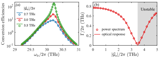
Figure S1: (a) Conversion efficiency $T_{ac}$ (solid curves) and $\mathcal{T}_{ac}$ (circles) as functions of the frequency of the IR signal $\omega_{\text{ir}}$ for different values of $|\mathcal{G}_{a}|$ at $\omega=\omega_{\text{ir}}$, obtained by Eq. (S8) via the response method and Eq. (S20) via the power spectrum method, respectively. (b) The bandwidth $\Gamma$ versus the enhanced collective optomechanical coupling strength $|\mathcal{G}_{a}|$. Other parameters are $\Delta=-\omega_{b}$, $\omega_{b}/2\pi=\omega_{c}/2\pi=30\,\text{THz}$, $\kappa_{a}/2\pi=30\,\text{THz}$, $\kappa_{c}/2\pi=0.5\,\text{THz}$, $\gamma_{B}/2\pi=0.16\,\text{THz}$, $\varepsilon_{p}/2\pi=500\,\text{THz}$, $g_{c}/2\pi=0.1\,\text{GHz}$, and $N=10^{7}$. In panel (b), here the unstable region is marked with the grey shadow.

Based on Eq. (S14), the output field operator of the VIS mode is expressed as

$$\tilde{a}_{\text{out}}(\omega)=U_{11}(\omega)\tilde{a}_{\text{in}}(\omega)+U_{12}(\omega)\tilde{c}_{\text{in}}(\omega)+U_{13}(\omega)\tilde{B}_{\text{in}}(\omega)+U_{14}(\omega)\widetilde{a^{\dagger}}_{\text{in}}(\omega)+U_{15}(\omega)\widetilde{c^{\dagger}}_{\text{in}}(\omega)+U_{16}(\omega)\widetilde{B^{\dagger}}_{\text{in}}(\omega).$$ (S18)

And the output spectrum of the VIS mode is obtained as

$$S_{a,\text{out}}(\omega)=\int_{-\infty}^{+\infty}d\omega^{\prime}\left\langle\widetilde{a^{\dagger}}_{\text{out}}(\omega^{\prime})\tilde{a}_{\text{out}}(\omega)\right\rangle=\mathcal{T}_{ac}(\omega)S_{c,\text{in}}(\omega)+S_{a,\text{vac}}(\omega),$$ (S19)

where $S_{c,\text{in}}(\omega)$ is the input spectrum of the IR signal and $S_{a,\text{vac}}(\omega)\equiv|U_{14}(\omega)|^{2}+|U_{15}(\omega)|^{2}+|U_{16}(\omega)|^{2}$ is the output spectrum contributing from the vacuum noises. $\mathcal{T}_{ac}(\omega)$ is the conversion efficiency from IR signal to VIS range

$$\mathcal{T}_{ac}(\omega)=|U_{12}(\omega)|^{2}+|U_{15}(\omega)|^{2}.$$ (S20)

Eq. (S20) corresponds to the conversion efficiency from IR signal to VIS range at the first Stokes sideband under the condition of the blue-detuned pump field for $\omega=\omega_{\text{ir}}$.

To compare the conversion efficiencies of the IR signal obtained based on the optical response method and the power spectrum method, in Fig. S1(a) we plot the conversion efficiencies $T_{ac}$ and $\mathcal{T}_{ac}$ as functions of the frequency of the IR signal $\omega_{\text{ir}}$ for different values of $|\mathcal{G}_{a}|$ at $\omega=\omega_{\text{ir}}$ and $\Delta=-\omega_{b}=-\omega_{c}$. Here the solid curves and circles are obtained by Eqs. (S8) and (S20), respectively. We observe an excellent agreement between the conversion efficiencies $T_{ac}$ and $\mathcal{T}_{ac}$, which means that the results obtained based on the two methods are basically the same. Figure S1(b) shows the bandwidths $\Gamma$ of the conversion efficiencies, obtained via the optical response method and the power spectrum method.

S3 detailed discussion on the stability of the system

In this section, we will analyze the stability of the current system. Whether the system is stable or not depends on the sign of the real part of the eigenvalve of the coefficient matrix $M$ given in Eq. (S10). The positive real (negative real) and imaginary parts of the eigenvalue of the matrix $M$ correspond to the decay rate (gain rate) and eigen-frequency for the related diagonalized normal mode, respectively. When such a gain rate exists, the mean value of the operator of the related diagonalized normal mode diverges in the long-time limit resulting the unstability. The system is stable only if the real parts of all the eigenvalues of the coefficient matrix $M$ are positive [11, 12].

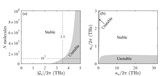
Figure S2: (a) The stability diagram with respect to the enhanced collective optomechanical coupling strength $|\mathcal{G}_{a}|$ and the number of the molecules $N$ at $\kappa_{a}/2\pi=30\,\text{THz}$ and $\kappa_{c}/2\pi=0.5\,\text{THz}$. (b) The stability diagram with respect to the decay rates $\kappa_{a}$ and $\kappa_{c}$ at the optimal coupling strength $|\mathcal{G}_{a}^{(*)}|\simeq\sqrt{(G_{c}^{2}|\eta_{c}^{-1}|+\kappa_{c}\gamma_{B}|\eta_{B}|)\kappa_{a}|\eta_{a}|/\kappa_{c}}$ and $N=10^{7}$. Other parameters are $\Delta=-\omega_{b}$, $\omega_{b}/2\pi=\omega_{c}/2\pi=30\,\text{THz}$, $\gamma_{B}/2\pi=0.16\,\text{THz}$, $\varepsilon_{p}/2\pi=500\,\text{THz}$, and $g_{c}/2\pi=0.1\,\text{GHz}$.

In Fig. S2(a), we show the stability diagram with respect to the enhanced collective optomechanical coupling strength $|\mathcal{G}_{a}|$ and the number of the molecules $N$, where other parameters are $\Delta=-\omega_{b}$, $\omega_{b}/2\pi=\omega_{c}/2\pi=30\,\text{THz}$, $\kappa_{a}/2\pi=30\,\text{THz}$, $\kappa_{c}/2\pi=0.5\,\text{THz}$, $\gamma_{B}/2\pi=0.16\,\text{THz}$, $\varepsilon_{p}/2\pi=500\,\text{THz}$, and $g_{c}/2\pi=0.1\,\text{GHz}$. The result indicates that the system is stable in the white area. For example, the system is stable at $N=10^{7}$ when $|\mathcal{G}_{a}|/2\pi<3.5\,\text{THz}$. At the case of the blue-detuned pump field $\Delta=-\omega_{b}$ and the resonance case $\omega_{\text{ir}}=\omega_{b}=\omega_{c}$, the maximum conversion efficiency of the IR signal is obtained at the optimal coupling strength $|\mathcal{G}_{a}^{(*)}|\simeq\sqrt{(G_{c}^{2}|\eta_{c}^{-1}|+\kappa_{c}\gamma_{B}|\eta_{B}|)\kappa_{a}|\eta_{a}|/\kappa_{c}}$. Figure S2(b) shows the stability diagram with respect to the decay rates $\kappa_{a}$ and $\kappa_{c}$ at the optimal coupling strength $|\mathcal{G}_{a}^{(*)}|$ and $N=10^{7}$. We observe that the system is stable in the white area.