Error Mitigated Metasurface-Based Randomized Measurement Schemes

Abstract

Estimating properties of quantum states via randomized measurements has come to play a significant role in quantum information science. In this paper, we design an innovative approach leveraging metasurfaces to perform randomized measurements on photonic qubits, together with error mitigation techniques that suppress realistic metasurface measurement noise. Through fidelity and purity estimation, we confirm the capability of metasurfaces to implement randomized measurements and the unbiased nature of our error-mitigated estimator. Our findings show the potential of metasurface-based randomized measurement schemes in achieving robust and resource-efficient estimation of quantum state properties.

I Introduction

Quantum processors [1] exploit the principles of quantum entanglement and quantum superposition to solve certain problems more efficiently than classical computers [2]. As these quantum processors scale up, characterizing the prepared quantum states becomes an increasingly intricate undertaking. Recently, protocols based on randomized measurements have been developed [3], such as the method of classical shadows [4]. These protocols, which typically involve repeated measurements on multiple copies of the same quantum state in random bases, have demonstrated high efficacy in predicting the properties of quantum states. However, the implementation of randomized measurements for photonic qubits [5, 6] requires the reconfiguration of the optical setup to modify the bases of measurements, thereby impeding practical scalability.

We have found that metasurfaces, two-dimensional surfaces composed of periodic sub-wavelength structured elements operating as order-selective diffractive grating [7], can be designed to project photons under random polarization bases. The metasurface is composed of several metagratings, each responsible for diffracting a unique pair of specific polarization states in two different directions. The working principle relies on the linear dependence of the geometric phase in metagratings. This allows for the manipulation of wavefronts using confined electromagnetic fields, which are based on plasmonic and Mie resonances. [8]. When metagratings associated with multiple polarization basis pairs are concatenated, they form an equivalent polarization-dependent diffractive grating. The metasurface directs photons to spatially separated locations depending on their polarization. This process naturally enables the randomized measurements of polarization-encoded photonic qubits. Importantly, a single metasurface is capable of measuring quantum states comprising an arbitrary number of qubits by sequentially projecting photons, demonstrating the scalability of our approach. In this work, we design a metasurface capable of conducting such randomized measurements and demonstrate its efficacy through numerical simulation of its optical properties.

Although theoretically, metasurfaces can execute noiseless randomized measurements, in practice, real-world implementations are susceptible to noise originating from design and fabrication constraints that can result in biased outcomes. To eliminate this noise-induced bias in estimating properties of quantum states, we analyze the physical origin of metasurface noise and construct a model that effectively explains the impact of noise on measurement outcomes.

This noise model is learned through metasurface calibration. Using the calibrated noise model, we develop an error mitigation technique capable of extracting true results from noisy outcomes via subsequent post-processing.

We have validated our protocol by performing numerical simulations of metasurfaces in the context of randomized measurements with applications on fidelity and purity estimation using classical shadows and statistical correlation of measurement outcomes [4]. Our results indicate that the protocol effectively mitigates the impact of noise and provides accurate estimates of quantum state properties.

In contrast to existing randomized measurement approaches for photonic qubits, our protocol negates the need for optical setup reconfiguration and allows easy scalability for multiple qubits. Furthermore, the proposed noise calibration and error mitigation technique efficiently address basis-dependent and photon loss noise, requiring only moderate experimental resources.

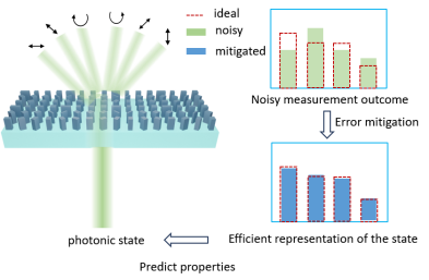
(a) Error mitigated randomized measurements using a metasurface

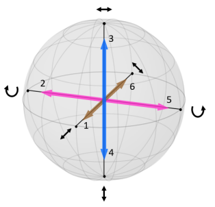
(b) measurement bases

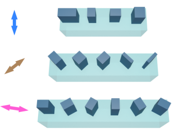
(c) Periodic elements of metasurface

Figure 1: Implementation of randomized measurements of photonic states using a metasurface. (a) Metasurface projects photons to one of six ports, based on a randomly selected polarization basis pair (H/V, H±V, LC/RC). This process constitutes a tomographically complete set of measurements. Input states, subject to measurement bases, yield noisy outcomes due to intrinsic metasurface noise. We adjust the weights of these outcomes according to a calibrated noise model from the metasurface. This allows the error-mitigated outcomes to approach ideal outcomes, which efficiently encode state information and reduce noise-induced bias in state property predictions. (b) The Positive Operator-Valued Measure (POVM) associated with a six-base metasurface is represented by $1/3\{|x^{\pm}\rangle\langle x^{\pm}|,|y^{\pm}\rangle\langle y^{\pm}|,|z^{\pm}\rangle\langle z^{\pm}|\}$, as illustrated in the Bloch sphere. (c) The measurement corresponding to each pair of POVMs is realized using a metagrating layer, functioning as a binary polarization-dependent diffractive grating.

The remainder of the paper is organized as follows: In Section II, we discuss the ability of metasurfaces to perform randomized measurements. Section III details our noise model, and Section IV outlines the noise calibration procedures. Section V introduces our error mitigation technique. In Section VI, we numerically implement the protocol for the estimation of quantum states via applications generating the classical shadows of $n$-qubit photonic states. Finally, Section VII summarizes our primary findings and suggests future research directions.

II Randomized measurements with metasurface

We begin by detailing the implementation of randomized measurements using metasurfaces under the formalism of the Positive Operator-Valued Measure (POVM) [9]. For a measurement involving $n$-qubits, the metasurface-associated POVM, denoted as $\mathbf{E^{\mathrm{global}}}$, takes the form $\mathbf{E^{\mathrm{global}}}=\mathbf{E}^{1}\times\cdots\times\mathbf{E}^{q}\times\cdots\times\mathbf{E}^{n}$. Here, each local set $\mathbf{E}^{q}$ (where $q\in[1,n]$) equals $\mathbf{E}$ and represents a POVM with $K$ positive-semidefinite elements that act only on the $q^{\mathrm{th}}$ qubit. A detailed explanation of the metasurface’s working principle, modelled as a measurement apparatus using POVMs, can be found in Appendix A.

The local set $\mathbf{E}$ comprises paired elements in the metasurface setup. This means that for any element $E_{(i,b)}$ in the set, there is another unique element $E_{(i,\bar{b})}$, such that $E_{(i,b)}+E_{(i,\bar{b})}=\frac{2}{K}I$. Each local POVM element $E_{(i,b)}$ is proportional to a rank-one projector $E_{(i,b)}=\frac{2}{K}|\phi_{(i,b)}\rangle\langle\phi_{(i,b)}|$, and the set of these should be tomographically-complete. Furthermore, in order for the randomized measurement schemes to be practical, the pure states $|\phi_{(i,b)}\rangle$ corresponding to elements in $\mathbf{E}$ need to form a quantum 2-design [10] (see Appendix B for additional details). Given these assumptions, we can write $\mathbf{E}$ as $\{E_{(i,0)},E_{(i,1)}\}_{i=1}^{K/2}$.

With the above conditions on $\mathbf{E}$, the metasurface can be considered to be a device performing two-outcome measurements in $K/2$ distinct bases. Each grating on the metasurface corresponds to a pair of POVM elements ${E_{(i,0)},E_{(i,1)}}$. Photons with different measurement readouts would be emitted in different directions from the grating and detected at spatially separated ports. Figure 1 provides an example for $K=6$

The first step in evaluating functions of a quantum system that is characterized by a $n$-qubit density matrix $\rho$ involves data collection from randomized measurements [11]. Specifically, we perform measurements defined by the POVM $\mathbf{E}^{\mathrm{global}}$ on $\rho$. The outcome $\mathbf{r}=[r^{1},\dots,r^{q}\dots,r^{n}]$ is obtained with probability $P_{\mathbf{r}}$, according to Born’s rule: $P_{\mathbf{r}}=\mathrm{Tr}(\rho\cdot E_{r^{1}}\otimes\cdots\otimes E_{r^{n}})$. The outcome for the $q^{\mathrm{th}}$ qubit, $r^{q}$, is a tuple $(i^{q},b^{q})$, where $i^{q}\in[1,K/2]$ represents the measurement basis, and the bit $b^{q}\in{0,1}$ represents the corresponding readout. This measurement process is repeated $N$ times, yielding the data set ${\mathbf{r}_{1},\cdots,\mathbf{r}_{N}}$. The subsequent step involves performing classical post-processing using the collected data, with the specific post-processing scheme dependent on the functions to be evaluated, as described in [4, 12, 13]. We discuss several specific post-processing schemes in detail in Section VI.

III Noise modelling

The above discussion assumed that the metasurface performs ideal noise-free randomized measurements. However, it is crucial to account for the inherent sources of measurement noise that are present in real metasurfaces. We model this noise here as general operations acting on the POVM elements. Specifically, we propose an effective noise operation $G$, which comprises a linear transformation, depicted by a transition matrix $A$ [14, 15], followed by a nonlinear operation $\Lambda$, which depends on the POVM set $\bf{E}$ and on the input state $\rho$. We will see later that the noise operations $A$ and $\Lambda$ have different sources. $A$ comes from a linear transformation of the POVM set $\mathbf{E}$, while $\Lambda$ is a result of photon loss. Thus, $G=\Lambda\circ A$. This model accommodates a wide range of noise types, and its effectiveness will be validated in Section IV. For now, we continue with a discussion of the general structure of our proposed noise model.

Since the dominant noise in $n$-qubit measurements conducted by metasurfaces is uncorrelated, the $K^{n}$-dimensional global transition matrix $A$ for the linear transformation decomposes into a tensor product form [14],

$$A=\bigotimes_{q=1}^{n}\Gamma^{q},$$ (1)

where $\Gamma^{q}=\Gamma$ for all $q\in[1,n]$, representing the $K$-dimensional transition matrix for the local POVM $\mathbf{E}$ of the $q^{\mathrm{th}}$ qubit. This then transforms the original POVM elements $E_{(i,b)}$ into noisy POVM elements $\tilde{E}_{(i,b)}$ according to the transition matrix $\Gamma$

$$\tilde{E}{(i,b)}=\sum_{(i^{\prime},b^{\prime})}\Gamma_{(i,b),(i^{\prime},b^{\prime})}E_{(i^{\prime},b^{\prime})}.$$ (2)

Here, the matrix element $\Gamma_{(i,b),(i^{\prime},b^{\prime})}$ is the probability of obtaining the measurement outcome $(i,b)$, given the idealized outcome $(i^{\prime},b^{\prime})$ in the absence of noise. To ensure that the generated set ${\tilde{E}_{(i,b)}}$ also constitutes a POVM, each column of $\Gamma$ must sum to one.

The dominant intrinsic noise associated with metasurfaces does not induce transitions between different bases, i.e., no coherent noise contributes to the metasurface measurements. Therefore, the transition matrix $\Gamma$ is block-diagonal, $\Gamma_{(i,b),(i^{\prime},b^{\prime})}=\delta_{i,i^{\prime}}\Gamma_{(i,b),(i,b^{\prime})}$, allowing it to be further decomposed into a direct sum form

$$\Gamma=\bigoplus_{i=1}^{K/2}\Gamma_{i},$$ (3)

where $\Gamma_{i}$ is the two-dimensional transition matrix that acts only on the pair of POVM elements $\{E_{(i,0)},E_{(i,1)}\}$.

By applying Born’s rule, the noisy probability distribution $\tilde{P}_{(\mathbf{i},\mathbf{b})}$ of measurement outcomes is then related to the noise-free probability distribution $P_{(\mathbf{i},\mathbf{b})}$ via the action of transition matrix $A=\Gamma^{\otimes n}$,

$$\tilde{P}_{(\mathbf{i},\mathbf{b})}=\sum_{\mathbf{i}^{\prime},\mathbf{b}^{\prime}}A_{(\mathbf{i},\mathbf{b}),\left(\mathbf{i}^{\prime},\mathbf{b}^{\prime}\right)}P_{(\mathbf{i^{\prime}},\mathbf{b^{\prime}})},$$ (4)

where $\mathbf{i}=[i^{1},\dots,i^{q},\dots,i^{n}]$ and $\mathbf{b}=[b^{1},\dots,b^{q},\dots,b^{n}]$, with $i^{q}\in[1,K/2]$ and $b^{q}\in\{0,1\}$ for all $q\in[1,n]$.

The nonlinear action $\Lambda$ depends not only on the noise-free POVM set $\mathbf{E}$, but also on the input state $\rho$. Hence, it generates the noisy probability distribution $\tilde{P}_{(\mathbf{i},\mathbf{b})}$ which depends nonlinearly on all the noise-free probabilities $\{P_{(\mathbf{i},\mathbf{b})}\}$.

We now move to a detailed examination of the specific intrinsic noise present in metasurfaces and its physical origin. It is important to note that the noise models we consider here are not due to defects or to imperfect experimental settings, but are inherited from the design of the metasurfaces.

III.1 Bit-flip and depolarizing noise

A metasurface consists of a finite number of discrete units. Due to the phase change discontinuity and boundary conditions arising from its finite size, readout errors can occur. This characteristic inherently introduces measurement noise. The most common type of noise can be modelled as a bit-flip, e.g., if a horizontally polarized photon is erroneously diffracted in a direction associated with vertical polarization.

Bit-flip errors may occur with a probability $p_{bf}$, and the outcome associated with the POVM element $E_{(i,b)}$ is correspondingly flipped to its paired outcome related to the POVM element $E_{(i,\bar{b})}$ [16]. In contrast, depolarizing errors lead to a situation in which, with a certain probability $p_{d}$, the photon is output with a uniformly random probability of $1/K$ from all detection ports [11].

These types of measurement noise derive from diverse physical sources. For instance, depolarizing noises can arise from a finite coupling strength between the photon and the measurement devices, resulting in weak (non-projective) measurement [17, 18]. In contrast, bit-flip errors may be attributed to the open boundary and discrete nature of the metasurfaces [19].

In metasurfaces, due to the pairing of the elements in the POVM, these two types of noises impact the POVM elements similarly and thus also affect the probability distributions similarly. Specifically, for measurement by a metasurface, a depolarizing error with rate $2p_{d}$ is equivalent to a bit-flip error with rate $p_{bf}$. We describe the impact of each error by a channel. For instance, the impact of bit-flip noise is described by the channel $\mathcal{E}_{d}\left(E_{(i,b)}\right)=p_{bf}(i)\cdot I+\left(1-2p_{bf}(i)\right)\cdot E_{(i,b)}$. The transition matrix elements of $\Gamma_{i}$ related to the two components of the channel are

$$\Gamma_{(i,b),\left(i,b^{\prime}\right)}=\left[1-p_{bf}(i)\right]^{\delta_{b,b^{\prime}}}\cdot p_{bf}(i)^{1-\delta_{b,b^{\prime}}},$$ (5)

where $p_{bf}(i)$ is the bit-flip error rate for the $i^{\mathrm{th}}$ basis.

III.2 Amplitude damping noise

Suppose a metasurface is positioned in the horizontal plane and photons are projected vertically towards the metasurface (see Figure 1(a)); the photon wavefront spreads across the metasurface. However, since the metasurface exhibits asymmetry in the horizontal plane, the resulting diffraction pattern depends on the spatial component of the polarization. This can lead to unevenly distributed measurement noise for a particular pair of polarizations. For instance, while the ’H’ (horizontal) polarization might be measured with high fidelity, the ’V’ (vertical) polarization could be more susceptible to being misread as ’H’. Such noise behaviour can be modelled as photons passing through an amplitude-damping quantum channel.

In other words, amplitude damping noise occurs when a photon that should ideally be projected to $E_{(i,1)}$ is instead projected to $E_{(i,0)}$ with probability $p_{ad}$. This error can be seen as a result of an asymmetric design between the ports associated with paired POVM elements.

When combined with typical bit-flip noise, the cumulative effect of these two types of amplitude damping and bit-flip noise lead to asymmetric bit-flip noise between a pair $\{E_{(i,0)},E_{(i,1)}\}$ with unequal bit-flip rates, a situation that is common for a 2D transition matrix $\Gamma_{i}$.

The amplitude damping noise on the POVM elements pair $\{E_{(i,1)},E_{(i,0)}\}$ can be described by a channel with a non-Hermitian Kraus operator [9] such that $\tilde{E}_{(i,0)}=E_{(i,0)}+p_{ad}(i)E_{(i,1)}$ and $\tilde{E}_{(i,1)}=\left(1-p_{ad}(i)\right)E_{(i,1)}$, and the associated transition matrix $\Gamma_{i}$ is given by

$$\Gamma_{i}=\left[\begin{array}[]{cc}1&p_{ad}(i)\\ 0&1-p_{ad}(i)\end{array}\right],$$ (6)

where $p_{ad}(i)$ is the amplitude damping error rate for the $i^{\mathrm{th}}$ basis.

III.3 Photon loss noise

Photon loss noise is a form of nonlinear noise, distinct from the linear transformations on POVM elements discussed so far. This type of noise can arise in several circumstances, such as when a photon is reflected due to a limited transmission rate, a photon detection port fails to detect the existence of a photon, or a photon emerges from a higher-order diffraction direction after coupling with the metasurfaces [8].

The photon loss rates $p_{pl}(i,b)$ that are associated with each detecting port $(i,b)$ may vary. Unequal photon loss rates for a pair of elements ${E_{(i,0)},E_{(i,1)}}$ in the POVM can result in the output string probability deviating from their true values.

At this point, we have proposed an effective noise model $G$ acting on the noise-free probabilities $P_{(\mathbf{i},\mathbf{b})}$. This model describes a sequence of possible transformations: first, a bit-flip/depolarizing operation, followed by an amplitude damping operation, and finally, a photon loss nonlinear operation. It’s important to emphasize that bit-flip and amplitude damping operations are commutative. Yet, as we’ll explore later, placing the nonlinear operation $\Lambda$ before $A$ is crucial to ensure consistency between error mitigation and the noise model. Hence, we maintain the sequence of noise operations as presented. The noisy probability distributions of measurement outcomes $\tilde{P}_{(\mathbf{i},\mathbf{b})}$ are then related to the ideal noise-free distribution $P_{(\mathbf{i},\mathbf{b})}$ by

$$\tilde{P}_{(\mathbf{i},\mathbf{b})}=G(\lambda)P_{(\mathbf{i},\mathbf{b})},$$ (7)

where $\lambda$ represents the noise rates for multiple noise sources.

The impact of these noises are modelled by applying transformations to the noise-free probability distribution, resulting in a noisy distribution. The error mitigation, discussed in section V, can be viewed as applying the inverse transformation to the noisy data. This allows for the extraction of true distributions from the noisy photon count distributions.

IV CALIBRATION OF INTRINSIC NOISES

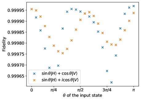
Figure 2: Evaluation of noise modelling and calibration: The calibrated noise model is utilized to predict outcomes, with fidelity calculated against real measured outcomes. The evaluations are conducted across various states, each with different relative amplitudes and phases. With fidelity values consistently exceeding 0.998, this suggests that the calibrated noise effectively models the intrinsic noise of the metasurface. Consequently, it validates the accuracy of the noise model we have constructed

This section outlines the method used to design the noise calibration experiment, and the protocol to determine the transition matrix $A$. In principle, we could perform a tomography-like experiment, such as quantum detector tomography, to learn all matrix elements of every noisy POVM element $\tilde{E}_{(i,b)}$ [20]. However, as the dimension increases, this task becomes highly resource-intensive. Alternatively, we can propose a noise model with parameters to be determined, fit these parameters using calibration data, and then verify the fitted model with additional experimental data. This process significantly reduces the cost of specifying the POVM.

Specifically, we adopt the noise models discussed in Section III. We consider uncorrelated noise models without contributions from coherent noise, i.e., we assume the linear part of the error model takes the form of Eq. (3), so that transitions are allowed only between paired POVM elements $\{E_{(i,0)},E_{(i,1)}\}$.

The calibration protocol proceeds as follows. We first perform measurements on $C$ input states, $\{|k\rangle\}_{k=1}^{C}$. The noise-free probabilities associated with each input state are easily calculated via Born’s rule. We then apply the total noise operation $G(\lambda)$ to these probabilities, where the vector $\lambda$ now represents the noise strength parameters to be determined. To obtain the noisy probabilities from the effective noise model, we denote the noisy outcome probabilities from the model as $\{\tilde{P}(k,\lambda)\}_{k=1}^{C}$, and the noisy outcome probabilities estimated empirically from calibration experiments as $\{\bar{P}(k)\}_{k=1}^{C}$. We use the fidelity $F_{p}$ of two classical probabilities $p$ and $q$ in order to quantify the closeness of the two outcomes

$$F_{pr}(p,q)=\left(\sum_{i}\sqrt{p_{i}q_{i}}\right)^{2}.$$ (8)

Given these definitions, the parameters $\lambda$ of the noise models are then obtained via the solution of the following optimization problem:

$$\lambda_{opt}=\mathrm{arg}\max_{0\leq\lambda_{i}\leq 1}\left[\sum_{k}F_{pr}\left(\bar{P}(k),\tilde{P}(k,\lambda)\right)\right].$$ (9)

To illustrate the protocol, we take the 6-port POVMs in Figure 1 as an example. For this case, $\mathbf{E}=1/3{|x^{\pm}\rangle\langle x^{\pm}|,|y^{\pm}\rangle\langle y^{\pm}|,|z^{\pm}\rangle\langle z^{\pm}|}$, where the POVM elements are eigenstates of Pauli $Z$, $X$, and $Y$ operators, i.e., $\mathbf{E}$ is the set of random Pauli measurements. Assuming the above error models and thus the functional form of $G(\lambda)$, we only need $6$ input states and the corresponding $6$ sets of probabilities to obtain $\lambda_{opt}$. We take the input states to be $|x^{\pm}\rangle$, $|y^{\pm}\rangle$, and $|z^{\pm}\rangle$. We generated calibration experimental data by performing COMSOL simulations [21] for three types of metagratings that are described in Appendix A. The metagrating parameters are summarized in Tables 2 and 3. The optimized noise parameters $\lambda_{opt}$ derived from the numerical solution of Eq. 9 for these metagratings are listed in Table 4.

To test the validity of the fitted error model $G(\lambda_{opt})$, we take $\psi_{xz}(\theta)=\mathrm{sin}(\theta)|H\rangle+\mathrm{cos}(\theta)|V\rangle$ and $\psi_{yz}(\theta)=\mathrm{sin}(\theta)|H\rangle+i\mathrm{cos}(\theta)|V\rangle$ as input states. We then calculate the fidelity of the outcome probabilities $F(\bar{P}(\theta),\tilde{P}(\theta,\lambda_{opt}))$ as a function of $\theta$, where $\tilde{P}(\theta,\lambda_{opt})$ is obtained from our fitted model $G(\lambda_{opt})$, and $\bar{P}(\theta)$ is from simulation of the metasurface using COMSOL. The results are shown in Fig (2), from which we can see the fidelity is above 0.999 for all values of $\theta$. This indicates validation of our generic measurement noise model, which includes bit-flip noise, amplitude-damping noise, and photon loss noise.

V Error mitigation

In this section, we develop error mitigation schemes to remove the bias induced by the previously discussed error models. The method we present applies to any randomized measurement protocol, since it operates on the level of measurement outcome probabilities. This is important because we aim to address basis-dependent measurement noise, which has previously proven challenging to handle [22, 23].

Regarding the linear components of the noise, once we have constructed the transition matrix $A$ via calibration, we can then apply the inverse of $A$ to infer noise-free probabilities $P_{(\mathbf{i},\mathbf{b})}$ from the empirical estimations of the noisy probabilities $\tilde{P}_{(\mathbf{i},\mathbf{b})}$, denoted as $\bar{P}_{(\mathbf{i},\mathbf{b})}$, which are subject to statistical errors

$$P_{(\mathbf{i},\mathbf{b})}=\sum_{\mathbf{i}^{\prime},\mathbf{b}^{\prime}}A_{(\mathbf{i},\mathbf{b}),\left(\mathbf{i}^{\prime},\mathbf{b}^{\prime}\right)}^{-1}\bar{P}_{(\mathbf{i}^{\prime},\mathbf{b}^{\prime})}.$$ (10)

In the case of photon loss noise, we can also develop an error mitigation scheme to infer $P_{(\mathbf{i},\mathbf{b})}$ from the empirical estimation $\bar{P}_{(\mathbf{i},\mathbf{b})}$ of $\tilde{P}_{(\mathbf{i},\mathbf{b})}$. If the photon loss rate associated with the POVM elements $\{E_{(i,b)}\}$ is $p_{pl}(i,b)$, then we can construct $P_{(\mathbf{i},\mathbf{b})}$ via a nonlinear renormalization procedure, given by

$$P_{(\mathbf{i},\mathbf{b})}=\frac{k_{(\mathbf{i},\mathbf{b})}}{\sum_{\mathbf{b}}k_{(\mathbf{i},\mathbf{b})}},$$ (11)

where $k_{(\mathbf{i},\mathbf{b})}$ is obtained from $\bar{P}_{(\mathbf{i},\mathbf{b})}$ as

$$k_{(\mathbf{i},\mathbf{b})}=\frac{\bar{P}_{\mathbf{i}}^{\mathbf{b}}}{\prod_{q=1}^{n}[1-p_{pl}(i_{q},b_{q})]}.$$ (12)

One can immediately notice from the above equation that if $\forall i$ we have $p_{pl}(i,0)=p_{pl}(i,1)$, then photon loss error would not affect the output string probability, i.e., $\tilde{P}_{(\mathbf{i},\mathbf{b})}=P_{(\mathbf{i},\mathbf{b})}$.

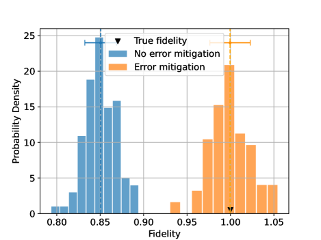
Figure 3: Estimated fidelity distribution of a five-qubit W state using classical shadows. The fidelity is estimated by ten thousand snapshots. Error-mitigated randomized measurements lead to unbiased estimation of fidelity (true fidelity = 1).

VI Evaluation of Protocol Performance: Estimating Fidelity and Purity

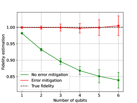
(a) W states for different numbers of qubits

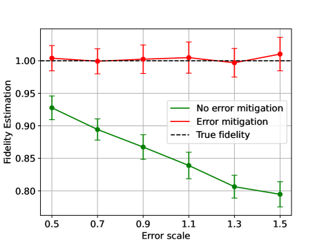
(b) W states for five qubits with adjusted noise levels.

Figure 4: Fidelity estimation of W states using classical shadows. The fidelity is evaluated by ten thousand classical shadows. Increased system size or higher error rates increase the noise effect on the final state, thereby decreasing fidelity. However, with the error mitigation protocol, the noise-induced bias in fidelity estimation can be effectively removed. The protocol shows scalability relative to (a) the number of qubits and (b) exhibits stability within a broad error range

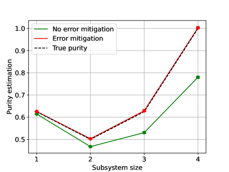
(a) W states for four qubits with different subsystem sizes

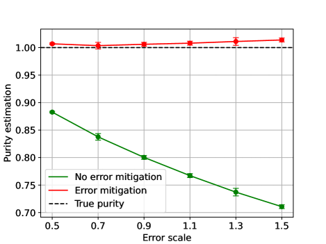
(b) W states for four qubits with adjusted noise levels.

Figure 5: Purity estimation of a four-qubit W state using randomized measurements. The purity is calculated as the weighted hamming distance between the ideal and the measured outcome. The purity of a subsystem (reduced density matrix) can quantify the entanglement of the entire system. (a) shows that the use of error-mitigated measurement outcomes results in an unbiased estimation of subsystem purity. (b) demonstrates the efficacy of the protocol across a broad noise regime

In this section, we evaluate the metasurfaces’ capability to perform randomized measurements, together with the effectiveness of error mitigation. Our specific goal is to estimate the properties of generalized W states for an n-qubit photonic system:

$$|w\rangle=(|10\ldots 0\rangle+|01\ldots 0\rangle+|00\ldots 1\rangle)/\sqrt{n}.$$ (13)

If one of $n$ qubits is lost, the state of the remaining system remains an $n-1$ qubit W state and is thus robust to particle loss [24, 25]. Given their utility in quantum teleportation, which typically employs photons as qubits, W states are adopted as the target state for analysis of the performance of our protocol.

Randomized measurements utilizing the metasurfaces are performed on the photonic W states, yielding noisy outcomes that are subsequently collected for error mitigation. The error-mitigated outcomes then undergo post-processing. We first apply this protocol to the case of classical shadows. The estimator $\hat{\rho}$ of the original density matrix $\rho$ is given by

$$\hat{\rho}_{k}=\hat{M}^{-1}(E_{\mathbf{r}_{k}}),$$ (14)

where the reconstruction map $\hat{M}^{-1}=\hat{M}^{-1}_{1}\otimes\hat{M}^{-1}_{2}\otimes\cdots\otimes\hat{M}^{-1}_{n}$ with $\hat{M}^{-1}_{i}(X)=3X-I$. $\hat{\rho}_{k}$ is referred as a classical shadow, which efficiently stores the information of the state and can be easily stored in a classical computer. One can verify that the classical shadow is an unbiased estimator of the original density matrix, in the sense that classical shadows averaged according to the probability distribution $P(\mathbf{r})$ converge to the original density matrix, i.e., $\mathbb{E}[\hat{\rho}]=\lim_{N\rightarrow\infty}1/N\sum_{k}\hat{\rho}_{k}=\rho$. For an observable $\hat{O}$, the estimation of the expectation value given the density matrix $\rho$ is then calculated via $\mathrm{Tr}(\hat{O}\rho)=1/N\sum_{k}\mathrm{Tr}(\hat{O}\hat{\rho}_{k})$. For the estimation of fidelity with the W state, we use

$$\mathbf{F}(\rho,|w\rangle\langle w|)=\mathbb{E}_{k}[\mathrm{Tr}(|w\rangle\langle w|\hat{\rho}_{k})].$$ (15)

In line with our established protocol, we numerically evaluate the fidelity of a five-qubit W state, utilizing ten thousand classical shadows collected through randomized measurements via a metasurface. This entire process is repeated one hundred times. The results, both noisy and error-mitigated fidelity distributions, are graphically represented in Fig. 3. It is noteworthy that the presence of noise leads to significant deviations in fidelity from the true value of one, indicating that the noisy results do not accurately represent the state information. In contrast, the error-mitigated fidelity distribution is now centered around the true value, demonstrating the effectiveness of our error mitigation protocol in rectifying measurement outcomes and effectively removing measurement bias stemming from noise.

We are also interested in evaluating the performance of the protocol across different system sizes and under various error regimes. In Fig. 4, ten thousand noisy and error-mitigated classical shadows of the W state are used to estimate the fidelity with the true W state, with panel (a) showing the dependence on the number of qubits in the W states, and panel (b) showing the dependence on the metasurface noise strength $\lambda$. Remarkably, we find that across a wide range of system sizes and errors, the error-mitigated method of classical shadows predicts a fidelity close to one, indicating that our error mitigation protocol offers an unbiased estimator of state properties in the presence of noise.

Alternatively, the measurements defined by the POVM can be considered as a process of sampling outcomes according to the probability associated with the POVM, which contains the information of the quantum state. Hence, properties of $\rho$ can be directly estimated from the collection of output strings $\{\mathbf{r}_{k}\}_{k=1}^{N}$. The level of entanglement of a quantum system is of broad interest in quantum information science. For multi-partite systems, it can be readily quantified by evaluating the purity of subsystems [26]. For a quantum system comprised of $n$ qubits denoted as $\mathcal{S}$, the purity of $P(\rho_{\mathcal{A}})$ defined on a subset $\mathcal{A}$ consisting of $n^{\prime}$ qubits is

$$P(\rho_{A})=\mathrm{Tr}[\rho^{2}_{\mathcal{A}}].$$ (16)

Here, $\rho_{\mathcal{A}}=\mathrm{Tr}_{\mathcal{S}\setminus\mathcal{A}}(\rho)$ is the reduced density matrix of subsystem $\mathcal{A}$. The purity $\mathrm{Tr}(\rho^{2}_{\mathcal{A}})$ of the subsystem can be calculated using the statistics of output strings of the measurements [13]

$$\mathrm{Tr}(\rho^{2}_{\mathcal{A}})=2^{n^{\prime}}\sum_{\mathbf{b},\mathbf{b}^{\prime}}(-2)^{D[\mathbf{b},\mathbf{b}^{\prime}]}\,\mathbb{E}_{\mathbf{i}}\left[P_{(\mathbf{i},\mathbf{b})}\,P_{(\mathbf{i},\mathbf{b^{\prime}})}\right].$$ (17)

Here $\mathbf{i}=[i_{1},i_{2},\dots,i_{n^{\prime}}]$ represents the measurement basis and $\mathbf{b}=[b_{1},b_{2},\dots,b_{n^{\prime}}]\in\{0,1\}^{n^{\prime}}$ represents the bit string of the readout restricted to the subsystem. $D[\mathbf{b},\mathbf{b^{\prime}}]$ is the Hamming distance between the two bit strings $\mathbf{b}$ and $\mathbf{b^{\prime}}$ and the probability $P_{(\mathbf{i},\mathbf{b})}$ is given y $P_{(\mathbf{i},\mathbf{b})}=\mathrm{Tr}[\rho\,E_{(i_{1},b_{1})}\otimes\cdots\otimes E_{(i_{n},b_{n})}]$. The expectation value $\mathbb{E}_{\mathbf{i}}$ is taken over all $K$ elements of the measurement basis.

Fig. 5 shows the subsystem purity evaluated for a four-qubit $W$ state using twenty thousand measurement outcomes. The left panel (a) illustrates that the original W state purity is accurately estimated using the error-mitigated outcomes. On the other hand, the right panel (b) demonstrates the protocol’s robustness across a wide range of error strength. These results indicate that not only does our protocol enable an unbiased estimation of quantum state properties but that it is also effective across a broad range of system sizes and levels of noise.

Through this comprehensive analysis, we have demonstrated that our error mitigation protocol efficiently improves the estimation of quantum state properties in the presence of noise, displaying its applicability and robustness for diverse observables and a broad range of noisy environments. This exemplifies the protocol’s potential for state property estimation for quantum computing and communication tasks.

VII Discussion

In summary, we have presented here an efficient protocol to perform randomized measurements using metasurfaces. We demonstrated the feasibility and scalability of the approach for photonic qubits, which eliminates the need for optical setup reconfiguration. To counter the effects of realistic metasurface noise sources in generating measurement noise, we showed how to establish an effective noise model and then use this to develop a corresponding error mitigation technique that ensures the accuracy of measurement outcomes to a high fidelity. The study provides a promising approach for robust and resource-efficient photonic quantum state property estimations.

In the current work, our primary focus was on the intrinsic noise associated with metasurfaces. This inherent noise includes unwanted diffraction and photon loss, phenomena that persist even under flawless metasurface fabrication and that typically exhibit a stochastic nature. Fabrication imperfections, on the other hand, tend to result in deviations from the desired measurement basis. It is important to note that our measurement bases are tomographically complete. This means that it is possible to calibrate the coherent measurement noise and to model its impact on the measurement outcomes, thereby facilitating the mitigation of noise induced by fabrication imperfections as well.

Some randomized measurement protocols need nonlocal measurements. These involve state manipulation via an operation capable of generating entanglement prior to measurements [3]. However, metasurfaces are capable of achieving multi-photon interference [7], a characteristic that enables nonlocal measurements. So we expect that the schemes described in this paper can be generalized to protocols requiring nonlocal randomized measurements, such as Clifford measurement-based classical shadow of quantum states.

In this work, we have described all necessary procedures to validate the proposed protocol with current quantum photonic technologies. We expect that experimental implementation with small numbers of photons is readily implementable and could lead to additional refinements and extensions of the protocol as metasurface noise calibration is implemented in practice on real systems.

VIII Acknowledgements

The authors thank Ying Li for valuable discussions. ZZ acknowledges the support from the Royal Society scholarship. LX and MR acknowledge support from the UK Research and Innovation Future Leaders Fellowship (MR/T040513/1). YP, HR, and KBW were supported by the U.S. Department of Energy, Office of Science, National Quantum Information Science Research Centers, and Quantum Systems Accelerator.

Appendix A Design and characterization of metasurface

The guiding principle in our metasurface design is to create a metasurface that projects photons under randomly chosen basis pairs of H/V, H$\pm$V, LC/RC. Our design involves a metasurface composed of periodic Si nanodisks, the parameters of which are tuned to optimize measurement efficiency. We use numerical simulations to assist the metasurface design.

For an incident wavelength of 1550nm as an example, the nanodisks are designed to have a height $h_{0}=800$ nm and periodicity $p_{0}=800$ nm. We then scan the width and depth of the nanodisks along the x- ($D_{x}$) and y- axes ($D_{y}$), calculating the corresponding optical properties of the metasurfaces. Fig. 6 displays the transmission and phase change spectra under x- and y-polarised plane waves while altering the width and depth of the nanodisks. The design of nanodisks is optimized to enhance both transmission rate and phase change. Due to the excitations of Mie-type electric and magnetic dipole resonances within the nanodisks and their interference, the backward scattering is strongly suppressed, leading to distinct phase changes along the x and y axes and forming a birefringent film with high transmission.

In order to separate photons with opposite polarization into +1 and -1 diffraction orders, we leverage the spatial linear dependence of the geometric phase on the transverse position of metagratings (along the x-axis). We utilize the genetic algorithm (AGA) to carefully select the geometric parameters of each unit to arrange a gradient phase distribution of two orthogonal states ($\phi_{1}$ and $\phi_{2}$) along the x-axis with high transmission. The unit size is 750 $\times$ 800 nm. Eventually, we successfully designed metagratings that can separate three pairs of orthogonal states (HV, H$\pm$V, and RCLC), illuminating into different angles with 4$\times$1, 5$\times$1, and 6$\times$1 meta-atoms as periodic units (as shown in the figure). By assembling these metagratings, we can form metasurfaces that distinguish three pairs of orthogonal states into different diffractive angles, leading to six ports for the characterization of quantum states (as shown in Fig. 1(c)).

The detailed parameters of the metasurface design are listed in Table 1. Given the current experimental capabilities, it is feasible to fabricate a metasurface with these parameters. With this design, we numerically characterize the measurement efficiency, as shown in Table 2. The data used for noise calibration are listed in Table 3, and the calibrated noise rate can be found in Table 4.

The transmission and phase change spectra, obtained while adjusting the width and depth of the nanodisk, are calculated using Rigorous Coupled-Wave Analysis (RCWA) [27]. RCWA is a frequency-domain modal method based on the decomposition of a periodic structure and the pseudoperiodic solution of Maxwell’s equations in terms of their Fourier expansions [28].

The optical properties of metagratings are computed using the finite element method via COMSOL Multiphysics 6.0 software [21].

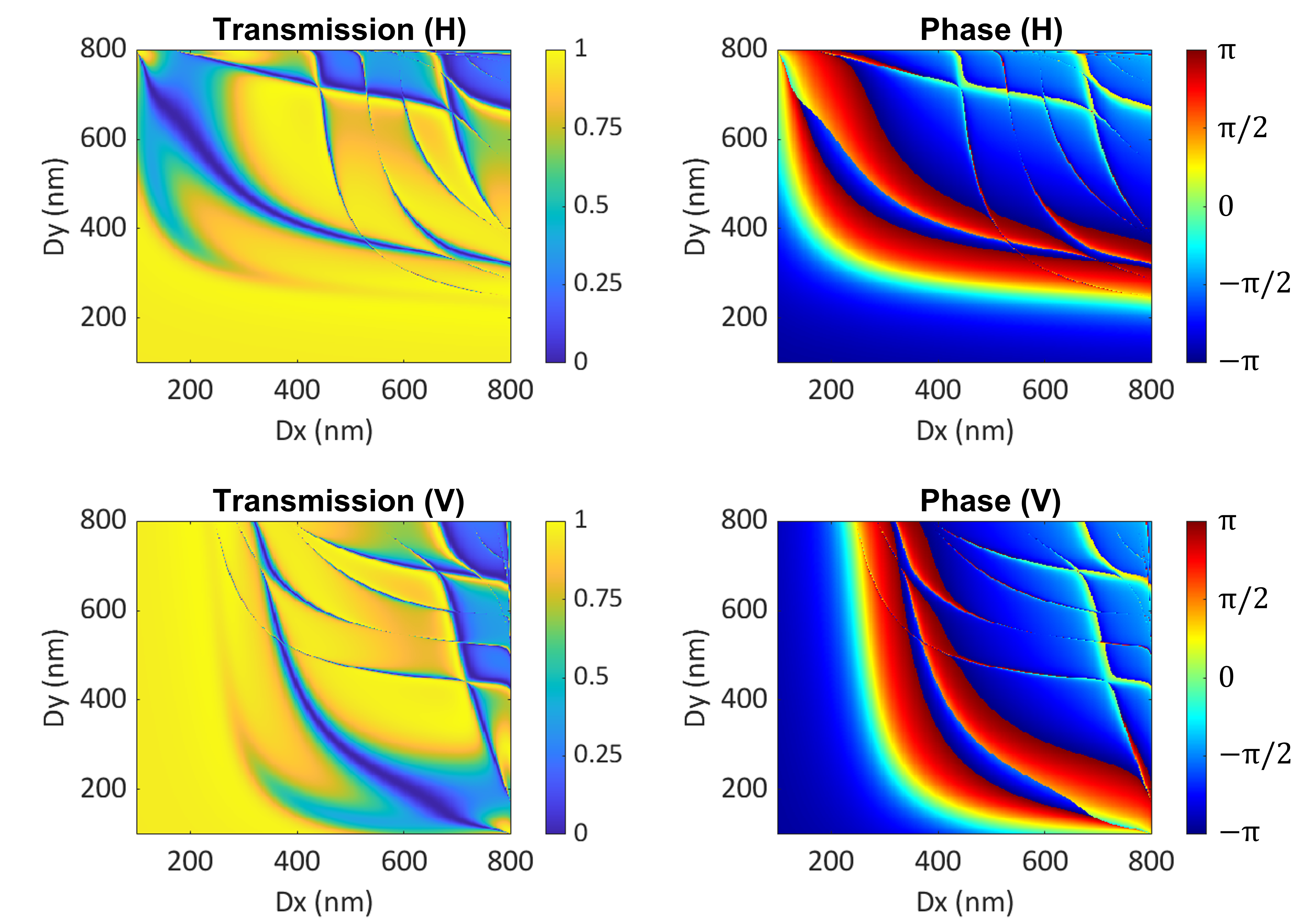
Figure 6: The transmission and phase change spectra of metasurfaces composed of nanodisks under x- (H) and y-polarised (V) plane wave, while tuning the width and depth of the nanodisks. The geometry of nanodisks is chosen to optimize the transmission rate and phase change.

Grating		1	2	3	4	5	6
HV	Dx (nm)	570	253	340	328
	Dy (nm)	264	285	236	347
	$\theta$	0	0	0	0
H±V	Dx (nm)	257	320	341	111	397
	Dy (nm)	375	314	266	400	102
	$\theta$	45	45	45	45	45
RCLC	Dx (nm)	355	355	355	355	355	355
	Dy (nm)	253	253	253	253	253	253
	$\theta$	0	30	60	90	120	150

Table 1: The geometric parameters of three metagratings. D_x and D_y are separately the width and depth of the nanodisk. $\theta$ is the rotation angle between the geometric and x axes.

Incident polarization		H	V	H+V	H-V	RC	LC
Grating HV	T+1,0	0.76556	0.01533	0.39063	0.39026	0.39053	0.39037
	T-1,0	0.01058	0.84082	0.42521	0.42619	0.4256	0.4258
Grating H$\pm$V	T+1,0	0.36103	0.36608	0.69704	0.03006	0.39121	0.33588
	T-1,0	0.40301	0.43212	0.05635	0.7788	0.40897	0.42618
Grating RCLC	T+1,0	0.38659	0.38188	0.39676	0.37172	0.00028	0.76819
	T-1,0	0.3874	0.38048	0.37189	0.39599	0.7676	0.00028

Table 2: The transmission of diffraction order +1,0 and -1,0 under the illumination of plane waves with different polarization states on three types of gratings.

	Ouput photon count
Incident polarization (input 10k photons)	H	V	H+V	H-V	RC	LC
H	2552	35	1203	1343	1291	1289
V	51	2803	1220	1440	1268	1273
H+V	1302	1417	2323	188	1240	1323
H-V	1301	1421	100	2596	1320	1239
RC	1302	1419	1304	1363	2559	1
LC	1301	1419	1120	1421	1	2561

Table 3: The calculated transmitted photon numbers on six ports with ten thousand incident photons with six bases (H, V, H+V, H-V, RC, LC). The numbers are calculated based on the simulated transmission of diffraction order +1,0 and -1,0 of three types of gratings.

Noise rate	H	V	H+V	H-V	RC	LC
Effective bit-flip	0.012466	0.012466	0.054692	0.054692	0.000383	0.000383
Amplitude damping	7.14E-03	7.14E-03	0	0	1.46E-05	1.46E-05
Photon loss	0.223475	0.144225	0.275352	0.162548	0.234566	0.228934

Table 4: Calibrated noise rate

Appendix B MEASUREMENT CHANNEL AND QUANTUM 2-DESIGN

In this section, we demonstrate that the quantum channel corresponding to the measurements defined by the positive operator-valued measure (POVM) $\mathbf{E}$ behaves as a depolarizing channel when $\mathbf{E}$ forms a quantum 2-design. This result, while extensively examined through the lens of representation theory, is briefly derived here for the sake of comprehensiveness.

We begin by defining a quantum 2-design. Consider a set of vectors $\{|\phi_{i}\rangle\}_{i=1}^{K}$, residing within the unit sphere $\mathbb{S}^{d}$ of a $d$-dimensional Hilbert space $\mathcal{H}^{d}$. This set is said to form a quantum 2-design if it meets the following condition [29]

$$\frac{1}{K}\sum_{i=1}^{K}|\phi_{i}\rangle\langle\phi_{i}|^{\otimes 2}=\int_{\mathbb{S}^{d}}|\phi\rangle\langle\phi|^{\otimes 2}d\mu(\phi),$$ (18)

where $d\mu(\phi)$ is the uniform spherical measure defined on $\mathbb{S}^{d}$ [30]. A simple criterion for testing whether a set of states forms a quantum 2-design is given by the following equation [10]

$$\sum_{k,k^{\prime}}\left|\left\langle\phi_{k}\mid\phi_{k^{\prime}}\right\rangle\right|^{4}/K^{2}=2/\left(d^{4}+d^{2}\right).$$ (19)

The Haar integral in Eq. 18 can be evaluated using results from representation theory [31] to give

$$\int_{\mathbb{S}^{d}}|\phi\rangle\langle\phi|^{\otimes 2}d\mu(\phi) =\left(\begin{array}[]{c}d+1\\ 2\end{array}\right)^{-1}\Pi_{\mathrm{Sym}^{(2)}}$$ (20)

$$=\left(\begin{array}[]{c}d+1\\ 2\end{array}\right)^{-1}\frac{I+W}{2},$$

where $\Pi_{\mathrm{Sym}^{(2)}}$ is the projector onto the symmetric subspace of $\mathcal{H}^{d}\otimes\mathcal{H}^{d}$, and $W$ is the swap operator defined on $\mathcal{H}^{d}\otimes\mathcal{H}^{d}$, i.e. $W|\phi_{i}\rangle\otimes|\phi_{j}\rangle=|\phi_{j}\rangle\otimes|\phi_{i}\rangle,\forall|\phi_{j}\rangle,|\phi_{i}\rangle\in\mathcal{H}^{d}$.

For randomized measurements of a single qubit, we can evaluate the measurement channel $\hat{M}$ defined by the quantum 2-design POVM $\mathbf{E}$ using the above results

$$\hat{M}(\rho) =\frac{1}{K}\sum_{i=1}^{K}\mathrm{Tr}\left(\rho|\phi_{i}\rangle\langle\phi_{i}|\right)|\phi_{i}\rangle\langle\phi_{i}|$$ (21)

$$=\mathrm{Tr}_{1}\left[(\rho\otimes I)\cdot\left(\frac{1}{K}\sum_{i=1}^{K}|\phi_{i}\rangle\langle\phi_{i}|^{\otimes 2}\right)\right]$$

$$=\frac{I+\rho}{3},$$

where $\mathrm{Tr}_{1}$ denotes the partial trace over the first copy of system and we take $d=2$ for the single qubit case. This allows us to invert the measurement channel as$\hat{M}^{-1}(X)=3X-I$, which is the same as in the unitary-based classical shadows, as expected.

In the case of a single qubit, the quantum 2-designs can be mapped to spherical 2-designs on the Bloch/Stokes sphere [32, 11]. The projectors in the POVM for $K=6$, $8$, $12$ are depicted as vectors on the Bloch sphere in Fig. 7. We have also conducted numerical simulations to estimate the fidelity of multi-qubit W-state including noise using POVMs with $K=6$, $8$, $12$, with the results presented in Fig. 8. The performance of the different POVMs is quite similar, although the 8-port POVM shows a slight advantage in the absence of error mitigation, and the 6-port POVM performs marginally better when error mitigation is employed.

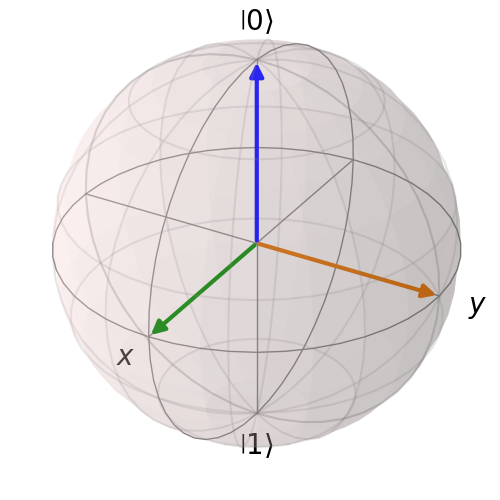
(a) 6 ports

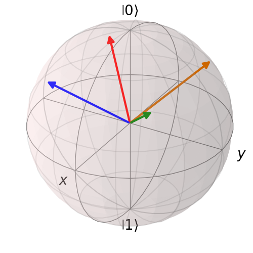
(b) 8 ports

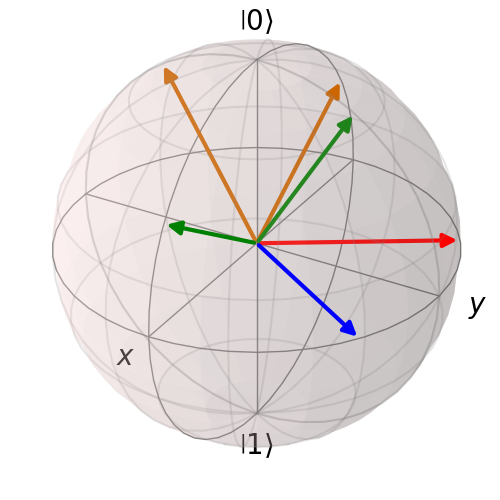
(c) 12 ports

Figure 7: Visulazation of the measurement bases of metasurface in the Bloch sphere. Vectors $|v\rangle$, corresponding to the POVM element $\frac{2}{K}|v\rangle\langle v|$, are represented in the Bloch sphere. Combined with their opposing vectors, which are omitted here, they constitute a complete POVM set. The arrangements of these vectors adhere to a spherical 2-design, thereby resulting in the formation of geometric configurations: Octahedron (6 ports), Hexahedron (8 ports), and Icosahedron (12 ports).

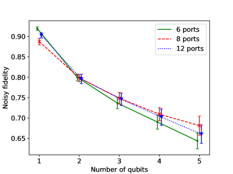
(a) A subfigure

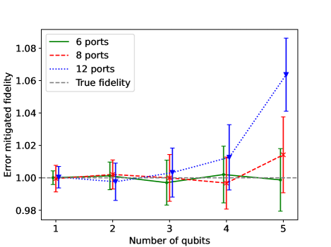
(b) A subfigure

Figure 8: Evaluation of W-State Fidelity through Randomized Measurements Using Various Metasurface Configurations. Metasurfaces, designed based on a spherical 2-design in the Stokes sphere, with different numbers of polarization measure bases (6, 8, and 12), produce valid randomized measurements due to their proven equivalence to a quantum 2-design [See Appendix B]. (a) In the presence of noise, metasurfaces with more of ports exhibit enhanced robustness. (b) Error mitigation is feasible across all port numbers, yet it is most effective with metasurfaces featuring six ports.

(a)

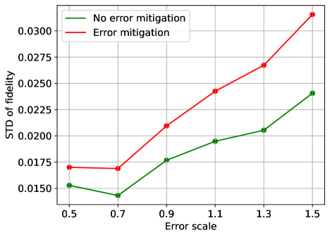
(b)

Figure 9: Quantifying Sample Complexity in Error Mitigation Protocols. The implementation of error mitigation techniques effectively eliminates noise-induced bias, albeit at the cost of increasing the standard deviation (STD) of the estimation, thus highlighting an increase in sample complexity. The fidelity STD of error mitigation is approximately 1.5 times higher compared to those without error mitigation, suggesting that the additional resources required for error mitigation implementation are justifiable

References

- Feynman [1982] R. P. Feynman, Simulating physics with computers, International Journal of Theoretical Physics volume 227, 109 (1982).
- Shor [1994] P. Shor, Algorithms for quantum computation: discrete logarithms and factoring, in Proceedings 35th Annual Symposium on Foundations of Computer Science (1994) pp. 124–134.
- Elben et al. [2023] A. Elben, S. T. Flammia, H.-Y. Huang, R. Kueng, J. Preskill, B. Vermersch, and P. Zoller, The randomized measurement toolbox, Nature Reviews Physics 5, 9 (2023).
- Huang et al. [2020] H.-Y. Huang, R. Kueng, and J. Preskill, Predicting many properties of a quantum system from very few measurements, Nature Physics 16, 1050 (2020).
- Zhang et al. [2021] T. Zhang, J. Sun, X.-X. Fang, X.-M. Zhang, X. Yuan, and H. Lu, Experimental quantum state measurement with classical shadows, Phys. Rev. Lett. 127, 200501 (2021).
- Struchalin et al. [2021] G. Struchalin, Y. A. Zagorovskii, E. Kovlakov, S. Straupe, and S. Kulik, Experimental estimation of quantum state properties from classical shadows, PRX Quantum 2, 010307 (2021).
- Wang et al. [2018] K. Wang, J. G. Titchener, S. S. Kruk, L. Xu, H.-P. Chung, M. Parry, I. I. Kravchenko, Y.-H. Chen, A. S. Solntsev, Y. S. Kivshar, et al., Quantum metasurface for multiphoton interference and state reconstruction, Science 361, 1104 (2018).
- Chen et al. [2016] H.-T. Chen, A. J. Taylor, and N. Yu, A review of metasurfaces: physics and applications, Reports on progress in physics 79, 076401 (2016).
- Nielsen and Chuang [2010] M. A. Nielsen and I. L. Chuang, Quantum computation and quantum information (Cambridge university press, 2010).
- Gross et al. [2007] D. Gross, K. Audenaert, and J. Eisert, Evenly distributed unitaries: On the structure of unitary designs, Journal of mathematical physics 48 (2007).
- Nguyen et al. [2022] H. C. Nguyen, J. L. Bönsel, J. Steinberg, and O. Gühne, Optimizing shadow tomography with generalized measurements, Physical Review Letters 129, 220502 (2022).
- Elben et al. [2019] A. Elben, B. Vermersch, C. F. Roos, and P. Zoller, Statistical correlations between locally randomized measurements: A toolbox for probing entanglement in many-body quantum states, Physical Review A 99, 052323 (2019).
- Brydges et al. [2019] T. Brydges, A. Elben, P. Jurcevic, B. Vermersch, C. Maier, B. P. Lanyon, P. Zoller, R. Blatt, and C. F. Roos, Probing rényi entanglement entropy via randomized measurements, Science 364, 260 (2019).
- Maciejewski et al. [2020] F. B. Maciejewski, Z. Zimborás, and M. Oszmaniec, Mitigation of readout noise in near-term quantum devices by classical post-processing based on detector tomography, Quantum 4, 257 (2020).
- Geller [2020] M. R. Geller, Rigorous measurement error correction, Quantum Science and Technology 5, 03LT01 (2020).
- Smith et al. [2021] A. W. Smith, K. E. Khosla, C. N. Self, and M. Kim, Qubit readout error mitigation with bit-flip averaging, Science advances 7, eabi8009 (2021).
- Oreshkov and Brun [2005] O. Oreshkov and T. A. Brun, Weak measurements are universal, Physical review letters 95, 110409 (2005).
- Tamir and Cohen [2013] B. Tamir and E. Cohen, Introduction to weak measurements and weak values, Quanta 2, 7 (2013).
- Wu et al. [2018] K. Wu, P. Coquet, Q. J. Wang, and P. Genevet, Modelling of free-form conformal metasurfaces, Nature communications 9, 3494 (2018).
- Lundeen et al. [2009] J. S. Lundeen, A. Feito, H. Coldenstrodt-Ronge, K. L. Pregnell, C. Silberhorn, T. C. Ralph, J. Eisert, M. B. Plenio, and I. A. Walmsley, Tomography of quantum detectors, Nature Physics 5, 27 (2009).
- Multiphysics [1998] C. Multiphysics, Introduction to comsol multiphysics®, COMSOL Multiphysics, Burlington, MA, accessed Feb 9, 2018 (1998).
- Chen et al. [2021] S. Chen, W. Yu, P. Zeng, and S. T. Flammia, Robust shadow estimation, PRX Quantum 2, 030348 (2021).
- Koh and Grewal [2022] D. E. Koh and S. Grewal, Classical shadows with noise, Quantum 6, 776 (2022).
- Dür et al. [2000] W. Dür, G. Vidal, and J. I. Cirac, Three qubits can be entangled in two inequivalent ways, Physical Review A 62, 062314 (2000).
- Pradhan et al. [2008] B. Pradhan, P. Agrawal, and A. Pati, Generalized w-states and quantum communication protocols, arXiv preprint arXiv:0805.2651 (2008).
- Bose et al. [2001] S. Bose, I. Fuentes-Guridi, P. L. Knight, and V. Vedral, Subsystem purity as an enforcer of entanglement, Phys. Rev. Lett. 87, 050401 (2001).
- Moharam et al. [1995] M. Moharam, E. B. Grann, D. A. Pommet, and T. Gaylord, Formulation for stable and efficient implementation of the rigorous coupled-wave analysis of binary gratings, JOSA a 12, 1068 (1995).
- Hugonin and Lalanne [2021] J. P. Hugonin and P. Lalanne, Reticolo software for grating analysis, arXiv preprint arXiv:2101.00901 (2021).
- Scott [2006] A. J. Scott, Tight informationally complete quantum measurements, Journal of Physics A: Mathematical and General 39, 13507 (2006).
- Watrous [2018] J. Watrous, The theory of quantum information (Cambridge university press, 2018).
- Gross et al. [2015] D. Gross, F. Krahmer, and R. Kueng, A partial derandomization of phaselift using spherical designs, Journal of Fourier Analysis and Applications 21, 229 (2015).
- Foreman et al. [2015] M. R. Foreman, A. Favaro, and A. Aiello, Optimal frames for polarization state reconstruction, Physical review letters 115, 263901 (2015).