Improved Approximation Algorithms for Steiner Connectivity Augmentation Problems

Abstract

The Weighted Connectivity Augmentation Problem is the problem of augmenting the edge-connectivity of a given graph by adding links of minimum total cost. This work focuses on connectivity augmentation problems in the Steiner setting, where we are not interested in the connectivity between all nodes of the graph, but only the connectivity between a specified subset of terminals.

We consider two related settings. In the Steiner Augmentation of a Graph problem ($k$-SAG), we are given a $k$-edge-connected subgraph $H$ of a graph $G$. The goal is to augment $H$ by including links and nodes from $G$ of minimum cost so that the edge-connectivity between nodes of $H$ increases by 1. This is a generalization of the Weighted Connectivity Augmentation Problem, in which only links between pairs of nodes in $H$ are available for the augmentation.

In the Steiner Connectivity Augmentation Problem ($k$-SCAP), we are given a Steiner $k$-edge-connected graph connecting terminals $R$, and we seek to add links of minimum cost to create a Steiner $(k+1)$-edge-connected graph for $R$. Note that $k$-SAG is a special case of $k$-SCAP.

All of the above problems can be approximated to within a factor of 2 using e.g. Jain’s iterative rounding algorithm [12] for Survivable Network Design. In this work, we leverage the framework of Traub and Zenklusen [18] to give a $(1+\ln{2}+\varepsilon)$-approximation for the Steiner Ring Augmentation Problem (SRAP): given a cycle $H=(V(H),E)$ embedded in a larger graph $G=(V,E\cup L)$ and a subset of terminals $R\subseteq V(H)$, choose a subset of links $S\subseteq L$ of minimum cost so that $(V,E\cup S)$ has 3 pairwise edge-disjoint paths between every pair of terminals.

We show this yields a polynomial time algorithm with approximation ratio $(1+\ln{2}+\varepsilon)$ for $2$-SCAP. We obtain an improved approximation guarantee of $(1.5+\varepsilon)$ for SRAP in the case that $R=V(H)$, which yields a $(1.5+\varepsilon)$-approximation for $k$-SAG for any $k$.

1 Introduction

1.1 Background

The edge-connectivity of a graph is a common measure of the robustness of the network to edge failures. If a network is $k$-edge-connected, then it can sustain failures of up to $k-1$ edges without being disconnected. Many problems in the area of network design seek to construct a cheap network which satisfies edge-connectivity requirements between certain pairs of nodes.

This has given rise to many fundamental problems of interest in combinatorial optimization and approximation algorithms. One notable example is the Survivable Network Design Problem (SNDP). In SNDP, we are given a graph with non-negative costs on edges and a connectivity requirement $r_{ij}$ for each pair of vertices $i,j\in V$. The goal is to find a cheapest subgraph of $G$ so that there are $r_{ij}$ pairwise edge-disjoint paths between all pairs of vertices $i$ and $j$.

Jain [12] gave a polynomial time algorithm for SNDP based on iterative rounding, which achieves an approximation factor of 2. Despite its generality, this algorithm achieves the best-known approximation ratio for a variety of network design problems of particular interest. For example, when $r_{ij}=k$ for all $i,j\in V$, we obtain the weighted minimum cost k-edge-connected spanning subgraph problem, for which no better-than-2 approximation algorithm is known, even when $k=2$. However, for some special cases, such as the minimum Steiner tree problem, specialized algorithms have been developed to improve upon this ratio. Hence, a major question in the field of network design is: for which network connectivity problems can we achieve an approximation factor below 2?

Recently, there has been major progress towards addressing this question. Consider the special case of SNDP known as the Weighted Connectivity Augmentation Problem (WCAP), in which we seek to augment the edge-connectivity of a given graph by inserting a collection of links of minimum cost. Formally, we are given a graph $G=(V,E)$ and a $k$-edge connected spanning subgraph $H=(V,E(H))$. The edges in $L:=E\setminus E(H)$ are called links and have non-negative costs. The goal is to choose a subset of links $S\subseteq L$ of minimum cost such that $(V,E\cup S)$ is a $(k+1)$-edge-connected graph.

A solution to WCAP must include a link crossing each of the min-cuts of the given graph $H$. Since the minimum cuts of any graph can be represented by a cactus [8], it is enough to consider the WCAP problem for $k=2$ and when $H$ is a cactus. This is called the Weighted Cactus Augmentation Problem. In fact, for the purposes of approximation, the Weighted Cactus Augmentation Problem reduces further to the case where $H$ is a cycle (the so-called Weighted Ring Augmentation Problem WRAP) [10]. If $k$ is odd, WCAP reduces to the case where $k=1$ and $H$ is a tree, yielding the Weighted Tree Augmentation Problem (WTAP).

In a breakthrough result, Traub and Zenklusen [19] employed a relative greedy algorithm based on the work of [4] to give the first approximation algorithm with approximation ratio better than 2 for WTAP. In particular, they achieved an approximation ratio of $(1+\ln{2}+\varepsilon)$ for WTAP, thereby yielding the same result for WCAP when $k$ is odd. Shortly afterward, they improved upon this result, bringing the approximation factor down to $(1.5+\varepsilon)$ for WTAP [20] using a local search algorithm.

After this breakthrough for WTAP, Traub and Zenklusen turned to the general case of the Weighted Connectivity Augmentation Problem. In [18], they adapt the same local search method that was used for WTAP to give a $(1.5+\varepsilon)$-approximation algorithm for Weighted Ring Augmentation Problem. As discussed above, this gives a $(1.5+\varepsilon)$-approximation for general WCAP.

It is important to note that for the above problems, the parameter of interest is the global edge-connectivity of the graph. However, in many applications, we are not interested in connectivity between all nodes in the graph, but rather only the connectivity between a specified subset of “important” nodes called terminals.

In this paper, we develop algorithms for generalizations of WCAP to this Steiner setting. The most natural problem of interest is the problem of augmenting a $k$-edge-connected Steiner subgraph into a $(k+1)$-edge-connected Steiner subgraph in the cheapest possible way. We call this problem $k$-SCAP:

Problem 1.1 (k-Steiner Connectivity Augmentation Problem).

We are given a graph $G=(V,E\cup L)$ and a subset of terminals $R\subseteq V$ such that $H:=(V,E)$ has $k$ edge-disjoint paths between every pair of vertices in $R$. We are also given a cost function $c:L\to\mathbb{R}_{\geq 0}$.

The goal is to select $S\subseteq L$ of cheapest cost so that the graph $(V,E\cup S)$ has $k+1$ pairwise edge-disjoint paths between all pairs of nodes in $R$.

In [17], the authors achieve a $(1.5+\varepsilon)$-approximation for the problem of cheaply augmenting a given Steiner tree to be a 2-edge-connected Steiner subgraph. This is called the Steiner Tree Augmentation Problem, and is equivalent to 1-SCAP. However, until now, there were no known results in this vein for higher-connectivity augmentation in the Steiner setting.

There is another, simpler problem which is a Steiner generalization of WCAP. In the standard WCAP problem, we can only add links between pairs of vertices in the given graph. What if we are allowed to use links which join nodes outside the graph to be augmented? This is the Steiner Augmentation of a Graph problem ($k$-SAG).

Problem 1.2 (Steiner Augmentation of a Graph).

We are given a $k$-edge-connected graph $H=(R,E)$, which is a subgraph of $G=(V,E~{}\dot{\cup}~{}L)$. The links $L$ have non-negative costs $c:L\to\mathbb{R}_{\geq 0}$.

The goal is to select $S\subseteq L$ of cheapest cost so that the graph $H^{\prime}=(V,E\cup S)$ has $k+1$ pairwise edge-disjoint paths between $u$ and $v$ for all $u,v\in R$.

Notice that $k$-SAG is a special case of $k$-SCAP.

Figure 1: A 3-SAG instance is shown on the left, and a 3-SCAP instance is shown on the right. The shaded nodes are terminals $R$, the black edges denote the edges of $E$ and the dashed edges represent the links $L$. In both pictures, the blue dashed links form a feasible solution.

1.2 Our results

In this paper, we give the first approximation algorithm with approximation ratio better than 2 for 2-SCAP, and for $k$-SAG for any $k$. To do this we introduce and solve the Steiner Ring Augmentation Problem (SRAP).

Problem 1.3 (Steiner Ring Augmentation Problem).

We are given a cycle $H=(V(H),E)$, which is a subgraph of $G=(V,E~{}\dot{\cup}~{}L)$. The links $L$ have non-negative costs $c:L\to\mathbb{R}_{\geq 0}$. Furthermore, we are given a set of terminals $R\subseteq V(H)$.

The goal is to select $S\subseteq L$ of minimum cost so that the graph $H^{\prime}=(V,E\cup S)$ has $3$ pairwise edge-disjoint paths between $u$ and $v$ for all $u,v\in R$.

Figure 2: A SRAP instance where the black edges denote the given cycle, the dashed edges are the links, and the blue links form a feasible solution. The shaded nodes are the terminals $R$.

In terms of approximability, the Steiner Ring Augmentation Problem captures both WCAP and STAP as special cases, in the sense that an $\alpha$-approximation for SRAP implies the same guarantee for both WCAP and STAP. We show that it also implies improved approximation algorithms for 2-SRAP and $k$-SAG.

Lemma 1.4.

If there is an $\alpha$-approximation for SRAP, then there is an $\alpha$-approximation for $2$-SCAP. If there is an $\alpha$-approximation for SRAP when $R=V(H)$, then there is an $\alpha$-approximation for $k$-SAG.

Our main theorem is an improved approximation algorithm for SRAP.

Theorem 1.5.

There is a $(1+\ln{2}+\varepsilon)$-approximation algorithm for SRAP.

The ultimate goal of this line of work would be to achieve a better-than-2 approximation algorithm for $k$-SCAP for general $k$. Our result on SRAP implies an improved approximation for this problem when $k=2$.

Corollary 1.6.

There is a $(1+\ln{2}+\varepsilon)$-approximation algorithm for the 2-Steiner Connectivity Augmentation Problem.

The challenge of obtaining a result for $k$-SCAP when $k\geq 3$ is that the cuts to be covered are no longer necessarily minimum cuts in the given graph. Thus, there is no way to represent these in a cactus or ring structure, and new techniques would have to be developed to deal with this case.

However, in the case of $k$-SAG, we can replace $H$ with a cactus, and subsequently a ring without changing the structure of its minimum cuts. Hence, the $k$-SAG problem ultimately reduces to the special case of SRAP where all cycles nodes are terminals. In this case, we can employ the local search methodology introduced by Traub and Zenklusen [20] to achieve an improved approximation ratio of $(1.5+\varepsilon)$.

Theorem 1.7.

There is a $(1.5+\varepsilon)$-approximation algorithm for SRAP when $R=V(H)$. Hence there is a $(1.5+\varepsilon)$-approximation algorithm for the Steiner Augmentation of a Graph problem.

1.3 Related Work

There is a broad body of work on algorithms for network connectivity, for various notions of connectivity, and in both the weighted and unweighted settings. See [11] and [14] for two excellent surveys.

We focus on edge-connectivity. Jain’s iterative rounding algorithm achieves an approximation ratio of 2 for the general survivable network design problem [12] in the weighted setting. As discussed above, this implies a 2-approximation for minimum cost $k$-edge-connected spanning subgraph (min $k$-ECSS) by taking $r_{ij}=k$ for all pairs of nodes. This is the best currently known approximation ratio for this problem, and can be achieved through a variety of classical methods such as the Primal Dual method, see [21].

The Weighted Connectivity Augmentation Problem (WCAP) is a special case of min $k$-ECSS where there is a 0 cost $(k-1)$-edge-connected subgraph. In the case of augmenting a $k$-edge-connnected graph where $k$ is odd, WCAP reduces to the extensively studied Weighted Tree Augmentation Problem (WTAP). Even WTAP is known to be APX-hard and is NP-hard on various special cases such as when the given tree has diameter four [9][13].

The current best approximation ratio for WTAP is $(1.5+\varepsilon)$ due to Traub and Zenklusen in [20]. Their approach was inspired by the work of Cohen and Nutov [4] who gave a $(1+\ln{2})$-approximation for WTAP when the given tree has constant diameter. Improved ratios can be obtained in the unweighted case: the state of the art being a 1.393 approximation due to [2], which also holds for unweighted Connectivity Augmentation.

It is known that the natural linear programming relaxation for WTAP has integrality gap at most 2 and at least 1.5 [3]. Stronger formulations have been considered for WTAP: Fiorini et. al. introduced the ODD-LP [8] which can be optimized over in polynomial time, despite having exponentially many constraints. The ODD-LP has integrality gap at most $2-\frac{1}{2^{h-1}}$ for WTAP on instances where the given tree can be rooted to have height $h$ [16].

In the case that $k$ is even, WCAP reduces in an approximation preserving way to the Weighted Cactus Augmentation Problem. Traub and Zenklusen broke the barrier of 2 for this problem and gave a $(1.5+\varepsilon)$-approximation algorithm, matching the approximation ratio for WTAP [18].

Nutov [15] considered the node-weighted version of SNDP and provided a $O(k\log n)$-approximation for this problem, where $k$ is maximum connectivity requirement. This implies $O(\log n)$-approximations for the node-weighted versions of all the problems considered in this paper.

1.4 Preliminaries

Suppose $G=(V,E)$ is a graph with vertex set $V$ and edge set $E$. For a non-empty subset of vertices $C\subsetneq V$, the cut $\delta(C)$ consists of all edges in $E$ with one endpoint in $C$. For a subset $X\subseteq E$, we denote by $\delta_{X}(C):=\delta(C)\cap X$. A cut $C$ is a $k$-cut if $|\delta(C)|=k$.

The edge-connectivity $\lambda(u,v)$ between a pair of vertices $u,v\in V$ is the maximum number of edge-disjoint paths between $u$ and $v$ in $G$. Equivalently, $\lambda(u,v)=\lambda(v,u)$ is the minimum cardinality of a cut $\delta(C)$ with $u\in C$ and $v\not\in C$. A graph is said to be $k$-edge-connected if $\lambda(u,v)\geq k$ for all pairs $u,v\in V$. Given a subset of terminals $R\subseteq V$, we say that $G$ is Steiner $k$-edge-connected on $R$ if $\lambda(u,v)\geq k$ for all pairs of terminals $u,v\in R$.

Given a Steiner $k$-edge-connected graph $G=(V,E)$ on terminals $R$, let $r\in R$, and define

$$\mathcal{C}^{\prime\prime}=\{C\subseteq V\setminus r:|\delta(C)|=k,C\cap R\neq\emptyset\}$$

to be the family of $k$-cuts of $G$ which separate some terminal from $r$. We call the cuts in $\mathcal{C}$ dangerous cuts.

The family of dangerous cuts has nice structural properties. In particular, it is uncrossable, that is, if $A$ and $B$ are members of $\mathcal{C}$ with $A\cap B\neq\emptyset$ and neither contained in the other, then either

• $A\cap B$ and $A\cup B$ are members of $\mathcal{C}$, or

• $A\setminus B$ and $B\setminus A$ are members of $\mathcal{C}$.

The $k$-SCAP problem is a hitting set problem where the ground set is the collection links $L$, and the sets are $\delta(C)$ where $C\in\mathcal{C}^{\prime\prime}$. That is, a set of links which is a solution to this hitting set problem will cause the graph to become Steiner $(k+1)$-edge-connected. The link $\ell$ “covers” the dangerous cuts $C$ with $\ell\in\delta(C)$.

We now recall the SRAP problem.

See 1.3

We refer to the nodes in $R$ as terminals, and the nodes in $V\setminus R$ as Steiner nodes. We will also refer to $H$ as the ring to distinguish it from a generic cycle. It will be convenient to fix a root $r\in R$ of the ring and an edge $e_{r}\in E$ incident on $r$.

We now introduce some terminology which allows us to be phrase the SRAP problem as a covering problem on a collection of ring-cuts only. Indeed, given the ring $H=(V(H),E)$, denote the set of min-cuts of $H$ as:

$$\mathcal{C}^{\prime}=\{C\subseteq V(H)\setminus r:|\delta_{E}(C)|=2\}.$$

Since we are only interested in connectivity between the terminals, we only need to cover the subfamily of $\mathcal{C}^{\prime}$ which separates terminals.

Let

$$\mathcal{C}=\{C\subseteq V(H)\setminus r:|\delta_{E}(C)|=2,C\cap R\neq\emptyset\}.$$

We call the cuts in $\mathcal{C}$ dangerous ring-cuts. It is easy to see that this family is also uncrossable. Consider any solution $S$ to SRAP where $S\subseteq L$.

Definition 1.8.

A full component of a SRAP solution $S$, is a maximal subtree of the solution where each leaf is a ring node (that is, a vertex of $V(H)$), and each internal node is in $V\setminus V(H)$.

Any link-minimal SRAP solution can be uniquely decomposed into link-disjoint full components. We say that a full component “joins” the ring nodes that it contains.

Definition 1.9.

Let $S$ be a solution to SRAP. We say that a set $A\subseteq R$ is joined by $S$ if there is a full component with leaves $A$.

In fact, the feasibility of a solution is determined only by the sets of nodes that it joins.

Definition 1.10.

We say that a cut $C\in\mathcal{C}$ is covered by a solution $S$ if $A\cap C\neq\emptyset$ and $\bar{A}\cap C\neq\emptyset$ for some subset of ring nodes $A$ which are joined by a full component of $S$.

Lemma 1.11.

A solution $S$ is feasible for SRAP iff all dangerous ring-cuts are covered by $S$.

Proof.

Suppose that each dangerous ring-cut of $H=(V(H),E)$ is covered. That is, for each $C\in\mathcal{C}$, there is a full component of $S$ joining vertices $A\subseteq V(H)$ such that $A\cap C\neq\emptyset$ and $\bar{A}\cap C\neq\emptyset$. We will show that any cut $C^{\prime}\subseteq V$ which separates a pair of terminals has $\delta_{E\cup S}(C^{\prime})\geq 3$, thereby implying the existence of 3 pairwise edge-disjoint paths between all terminal pairs.

Consider the cut $C^{\prime}\cap V(H)$ obtained by restricting $C^{\prime}$ to $V(H)$. We may assume that $C^{\prime}\cap V(H)$ is a 2-cut, otherwise $\delta_{E}(C^{\prime})\geq 3$ already. Furthermore, note that $C^{\prime}\cap R\neq\emptyset$. Hence, $C^{\prime}\cap V(H)$ is a dangerous ring-cut, and there is some full component of $S$ covering it. This implies that $\delta_{S}(C^{\prime})\geq 1$ so $\delta_{E\cup S}(C^{\prime})\geq 3$ as desired.

For the reverse direction, suppose that $S$ is a feasible solution to SRAP. Consider any dangerous ring-cut $C\in\mathcal{C}$. We will show that there must be a path in $S$ from a node in $C$ to another ring node which is not contained in $C$, implying that there is some full component covering $C$. Since $\delta_{E\cup S}(C)\geq 3$, there must be a link $(u,v)\in S$ with $u\in C$ and $v\not\in C$. If $v$ is a ring node, we are done. Otherwise, the cut $C^{\prime}=C\cup v$ is another dangerous cut which is covered by $S$. Repeating this process eventually yields a path of links from a node in $C$ to a ring node outside $C$, hence the full component of $S$ containing this path covers $C$. ∎

1.5 Hyper-SRAP and the hyper-link intersection graph

We next introduce the Hyper-SRAP problem. We are given a ring $H=(V(H),E)$ with terminals $R\subseteq V(H)$, a root vertex $r\in R$, and a collection of hyper-links $\mathcal{L}\subseteq 2^{V(H)}$ with non-negative costs $c:\mathcal{L}\to\mathbb{R}_{\geq 0}$.

Again, let $\mathcal{C}=\{C\subseteq V(H):|\delta_{E}(C)|=2,r\not\in C,C\cap R\neq\emptyset\}$ be the set of dangerous ring-cuts, i.e. the set of min-cuts of the ring $H$ which separate some terminal from $r$. Let $\ell$ be a hyper-link. We say that a cut $C\in\mathcal{C}$ is covered by $\ell$ if $\ell\cap C\neq\emptyset$ and $\ell\cap\bar{C}\neq\emptyset$. A subset of hyper-links $F\subseteq\mathcal{L}$ is feasible if all cuts in $\mathcal{C}$ are covered. The Hyper-SRAP problem is to find a minimum cost subset of hyper-links so that all cuts in $\mathcal{C}$ are covered.

We will use the notion of the hyper-link intersection graph, an auxiliary graph which gives a useful characterization of feasibility for Hyper-SRAP. First, we define what it means for two hyper-links to be intersecting.

Definition 1.12.

A pair of hyper-links $\ell_{1}$ and $\ell_{2}$ are intersecting if they share a vertex, or there is a vertex in $\ell$ between two vertices in $\ell^{\prime}$ and a vertex of $\ell^{\prime}$ in between two vertices of $\ell$.

Given an instance of Hyper-SRAP with ring $H=(V(H),E)$ and hyper-links $\mathcal{L}$, we define the hyper-link intersection graph $\Gamma$ as follows. For each hyper-link $\ell\in\mathcal{L}$ there is a node $v_{\ell}$. Two nodes $v_{\ell_{1}}$ and $v_{\ell_{2}}$ are adjacent in the hyper-link intersection graph if and only if $\ell_{1}$ and $\ell_{2}$ are intersecting hyper-links.

For ring vertices $u,v\in V(H)$, we say that there is a path from $u$ to $v$ in $\Gamma$ if there is a path in $\Gamma$ from a hyper-link containing $u$ to a hyper-link containing $v$. It turns out that a solution $S$ to Hyper-SRAP is feasible if and only if there is a path between every pair of terminals in the hyper-link intersection graph when restricted to $S$. The following lemma is proved in section 6.

Lemma 1.13.

Suppose $(H,\mathcal{L},R)$ is an instance of Hyper-SRAP with root $r$ and intersection graph $\Gamma$. Then $S\subseteq\mathcal{L}$ is feasible iff for each terminal $r^{\prime}\in R$, there is a path between $r$ and $r^{\prime}$ in the hyper-link intersection graph restricted to $S$.

1.6 Effects of $\gamma$-restriction

Definition 1.14.

We say that a full component is $\gamma$-restricted if it joins at most $\gamma$ ring nodes. We say that a solution to SRAP is $\gamma$-restricted if it uses only $\gamma$-restricted full components. Analogously, we say an instance of Hyper-SRAP is $\gamma$-restricted if each hyper-link has size at most $\gamma$.

We show that up to a factor of $(1+\varepsilon)$, it suffices to find the best $\gamma$-restricted solution to SRAP for some constant $\gamma(\varepsilon)$. First, we recall the following result for Steiner trees. Given a Steiner tree solution $T$, a full component of is a subtree of $T$ whose leaves are terminals and whose non-leaves are non-terminals. A $\gamma$-restricted Steiner tree solution is a solution whose full components all have at most $\gamma$ terminals.

Lemma 1.15 (Borchers and Du [1]).

Let $\varepsilon>0$. Fix an instance of Steiner tree and let $T^{*}$ be the optimal Steiner Tree and $T_{\gamma}$ be the optimal $\gamma$-restricted Steiner tree. Then for $\gamma=2^{\lceil{{\frac{1}{\varepsilon}}}\rceil}$, we have

$$\frac{c(T_{\gamma})}{c(T^{*})}\leq 1+\varepsilon.$$

Now, we prove an analogous result for SRAP. For an instance of SRAP, let $S^{*}$ be the optimal solution and $S_{\gamma}$ be the optimal $\gamma$-restricted solution.

Lemma 1.16.

For all $\varepsilon>0$, there exists $\gamma(\varepsilon)=2^{\lceil{{\frac{1}{\varepsilon}}\rceil}}$ such that

$$\frac{c(S_{\gamma})}{c(S^{*})}\leq 1+\varepsilon.$$

Proof.

By the optimality of $S^{*}$, each full component of $S^{*}$ is minimum cost Steiner tree on the ring nodes $A$ that it joins, in the graph $(A\cup(V\setminus V(H)),L)$. By Lemma 1.15, there is a $\gamma$-restricted Steiner Tree with at most $(1+\varepsilon)$ times the cost. Applying this to each full component of $S^{*}$ yields a solution of cost at most $(1+\varepsilon)c(S^{*})$ which only has full components joining at most $\gamma$ ring nodes. ∎

We recall that the minimum cost Steiner tree problem can be solved in polynomial time when the number of terminals is constant.

Theorem 1.17 (Dreyfus and Wagner [7]).

The minimum Steiner tree problem can be solved in time $O(n^{3}\cdot 3^{p})$ where p is the number of terminals.

Because Lemma 1.11 shows that the feasibility of a solution only depends on the nodes that are joined by full components of $S$, we can effectively disregard the Steiner nodes outside the ring and observe that any instance of SRAP is equivalent instance of Hyper-SRAP in which the cost of a hyper-link $A$ is the minimum cost Steiner tree connecting $A$ in the graph $(A\cup(V\setminus V(H)),L)$. By Lemma 1.16, and Theorem 1.17, we can perform this reduction from an arbitrary SRAP instance to an instance of $\gamma$-restricted Hyper-SRAP in polynomial time while only losing a factor of $(1+\varepsilon)$ in the approximation ratio.

1.7 Directed solutions

Finally, we will make use of directed solutions to the SRAP problem. If $\vec{F}$ is a collection of directed links between pairs of vertices of the ring, then a dangerous ring-cut $C\in\mathcal{C}$ is covered by $\vec{F}$ if $\delta_{\vec{F}}^{-}(C)\neq\emptyset$, i.e. if there is an arc in $\vec{F}$ which enters $C$. Then $\vec{F}$ is a feasible directed solution if all dangerous ring-cuts are covered by $\vec{F}$. Analogously, if $S$ is a set of undirected links and $\vec{F}$ is a set of directed links then we will say that $S\cup\vec{F}$ is a feasible mixed solution if every dangerous ring-cut is covered by $S$ or by $\vec{F}$.

2 Technical Overview

The main contribution of this article is to prove Theorem 1.5.

See 1.5

We begin by illustrating in section 3, how this implies improved approximation guarantees for both 2-SCAP and $k$-SAG. Recall that in the $k$-SCAP problem, we are given a graph $H$ which is Steiner $k$-edge-connected on the terminal set $R$. We want to augment this graph by including additional links of minimum cost so that there exists $k+1$ pairwise edge-disjoint paths between every pair of terminals. This is equivalent to covering the dangerous cuts of $H$ with a minimum cost set of links.

Note that if $k$ is larger than the global edge-connectivity of $H$, then there may be exponentially many dangerous cuts. Indeed even when $R=\{s,t\}$, the number of minimum $\{s,t\}$-cuts in a graph $G$ on $n$ nodes may be exponential in $n$. This shows that for general $k$-SCAP, the set of cuts to be covered cannot be represented by a cactus structure which is efficiently computable (although it is true that there are polynomially many dangerous cuts up to containing the same subset of terminals [6], this is not sufficient for our purposes).

However, in the case of $k=2$, we show in section section 3 that we may take $H$ to be a globally 2-edge-connected graph rather than merely Steiner 2-edge-connected. This allows us to compactly represent the cuts to be covered by a cactus on a set of nodes, some of which are terminals. We then use the technique introduced by G’alvez et. al. [10] to replace the cactus with a ring by adding in links of 0 cost. This bring the problem into the SRAP framework. In the case of $k$-SAG, we are guaranteed that $H$ is $k$-edge-connected so we can directly replace $H$ with a cactus with the same cut structure. This yields:

See 1.4

In order to prove Theorem 1.5, we give a relative greedy algorithms which follows the methodology developed in [18] for the Weighted Ring Augmentation Problem. We first summarize this method and then illustrate the challenges that arise in the Steiner setting, and how we deal with them.

First we provide an overview of the algorithm which achieves an approximation ratio of $(1+\ln{2}+\varepsilon)$ for WRAP. The algorithm is a relative greedy algorithm which begins by computing an initial directed solution which is highly structured, then iteratively improves upon this solution through local moves. In each local move, a collection of links is added to the solution, and a collection of directed links are dropped from the initial solution. The algorithm repeats this process until the initial solution becomes empty.

For the initial structured solution, Traub and Zenklusen show that it is possible to compute in polynomial time an initial 2-approximate directed solution to WRAP which is a planar $r$-out arborescence $\vec{F}$ reaching all other vertices in the ring. This arborescence structure gives a condition for when a directed link $(u,v)$ is allowed to be dropped from this solution such that a) feasibility of the mixed solution is maintained throughout the algorithm, and b) in each iteration of the algorithm, progress is made in terms of reducing the overall cost.

Our relative greedy algorithm for SRAP follows this framework. However, there are several key ingredients which are needed to obtain the result in the Steiner setting.

First, we need an initial structured 2-approximate solution to SRAP. Note that in the SRAP problem, unlike in the standard Ring Augmentation Problem, the optimal solution may use links between Steiner nodes outside the ring in order to increase the connectivity between pairs of terminals in the ring. In section 4, we prove Theorem 2.1, which shows that there is always a directed 2-approximate solution which only consists of directed links in the ring, is only incident on terminals, and which can be found in polynomial time. In particular we show:

Theorem 2.1.

There is a polynomial time algorithm for SRAP which yields a directed solution $\vec{F}$ of cost at most $2\text{OPT}$ such that:

1. $\vec{F}$ is only incident on the terminals $R$

2. $(R,\vec{F})$ is an $r$-out arborescence.

3. $(R,\vec{F})$ is planar when $V(H)$ is embedded as a circle in the plane.

4. For any $v\in V$, no two directed links in $\delta^{+}_{\vec{F}}(v)$ go in the same direction along the ring.

We call a directed solution which satisfies the conditions in Theorem 2.1 an $\boldsymbol{R}$-special directed solution. The proof of Theorem 2.1 is significantly more involved than the the directed 2-approximation for standard WRAP. At a high level, we first demonstrate that there is a 2-approximate directed solution consisting of a collection of directed cycles on the ring nodes. Then, we prove a “cycle merging lemma” which allows us to iteratively merge these cycles to eventually obtain a feasible directed solution which is a single directed cycle of at most the cost. Once we have a solution of this form, we can shortcut over the Steiner nodes in the ring to obtain a directed cycle solution which only touches terminals, which can then be shortened to satisfy the properties in Theorem 2.1.

An $R$-special directed solution of this form is necessary because it allows us to leverage a decomposition result on directed solutions with respect to the optimum. Because of the decomposition result, it can be argued that every iteration of the algorithm will find an improving local move as long as the current solution is expensive.

Traub and Zenklusen prove a decomposition result of this kind to achieve the approximation algorithm for WRAP [18]. However, in our setting, the optimal solution consists of full components which may join an arbitrary number of vertices in the ring, rather than just links which join pairs of ring vertices. Hence, we prove Theorem 2.3, extending the decomposition result in [18] to hyper-links. First we need to define the notion of an $\alpha$-thin collection of hyper-links. Recall that $\mathcal{C}^{\prime}$ is the set of minimum cuts of the ring $H$ which do not include the root.

Definition 2.2.

A collection of hyper-links $K\subseteq\mathcal{L}$ is $\alpha$-thin if there exists a maximal laminar subfamily $\mathcal{D}$ of $\mathcal{C}^{\prime}$ such that for each $C\in\mathcal{D}$, the number of hyper-links in $K$ which cover $C$ is at most $\alpha$.

In the following theorem, for a collection of hyper-links $K$ and an $R$-special directed solution $\vec{F}_{0}$, the notation $\text{drop}_{\vec{F}_{0}}(K)$ denotes a set of directed links from $\vec{F}_{0}$ which can be dropped while preserving feasibility of $\vec{F}_{0}\cup K$. This will be defined formally in section 6.

Theorem 2.3 (Decomposition Theorem).

Given an instance of Hyper-SRAP $(H=(V(H),E),R,\mathcal{L})$, suppose $\vec{F}_{0}$ is an $R$-special directed solution and $S\subseteq\mathcal{L}$ is any solution. Then for any $\varepsilon>0$, there exists a partition $\mathcal{Z}$ of $S$ into parts so that:

• For each $Z\in\mathcal{Z}$, $Z$ is $\alpha$-thin for $\alpha=4\lceil{1/\varepsilon}\rceil$.

• There exists $Q\subseteq\vec{F}_{0}$ with $c(Q)\leq\varepsilon\cdot c(\vec{F}_{0})$, such that for all $f\in\vec{F}_{0}\setminus Q$, there is some $Z\in\mathcal{Z}$ with $f\in\text{drop}_{\vec{F}_{0}}(Z)$. That is, $\vec{F}_{0}\setminus Q\subseteq\bigcup_{Z\in\mathcal{Z}}\text{drop}_{\vec{F}_{0}}(Z)$.

We remark that the above decomposition theorem does not hold if $\vec{F}_{0}$ is a directed arborescence which is incident on Steiner nodes. This is why Theorem 2.1 establishing the existence of an $R$-special directed solution only touching terminals is crucial for the relative greedy algorithm to obtain the desired approximation guarantee.

In order to reduce a given instance of SRAP to an instance of Hyper-SRAP we also make use of Lemma 1.16, which allows us to only consider full components joining constantly many ring vertices, while only losing an arbitrarily small constant in the approximation ratio.

This allows us to convert a given instance of SRAP into an equivalent Hyper-SRAP instance efficiently. It also ensures that each local move of the algorithm runs in polynomial time. In each local move, the algorithm chooses amongst all $\alpha$-thin collections of hyper-links $K$, the choice which minimizes the ratio between the cost of the hyper-links in $K$, and the cost of the directed links which will be dropped as a result of adding $K$ to the solution. In section 8, we show that this operation can be performed in polynomial time as long as all hyper-links have size at most $\gamma$.

Theorem 2.4.

Given an instance of $\gamma$-restricted Hyper-SRAP, an $R$-special directed solution $\vec{F}_{0}$ and an integer $\alpha\geq 1$, there is a polynomial time algorithm which finds a collection of hyper-links $K$ minimizing

$$\frac{c(K)}{c(\text{drop}_{\vec{F}_{0}}(K))}$$

over all $\alpha$-thin subsets of hyper-links.

Theorems 2.1, 2.3, and 2.4 together are essentially enough to employ a relative greedy strategy to obtain a better-than-2 approximation for SRAP. Beginning with an $R$-special 2-approximate directed solution, we iteratively add to this solution a greedily chosen $\alpha$-thin collection of hyper-links in each step. When a particular collection of hyper-links $K$ is chosen to be added, the directed links in $\text{drop}_{\vec{F}_{0}}(K)$ are dropped from $\vec{F}_{0}$, and this process is repeated until $\vec{F}_{0}$ becomes empty. The relative greedy algorithm and its proof are described in section 5.

Additionally, in the case that all ring nodes are terminals, we can use the local search framework introduced in [20] to give an algorithm with an improved approximation guarantee of $(1.5+\varepsilon)$. Together with Lemma 1.4, this yields:

See 1.7

The key idea in the improvement is to not only consider dropping links from the initial directed solution, but to drop undirected links which were added in previous iterations by associating to each undirected link a witness set of directed links which indicate when it can be dropped. This is proved in section 9.

We are able to do this in the case that $V(H)=R$ because in this case, any feasible directed solution can be transformed into an $R$-special solution of at most the cost. However, this is not the case for general SRAP (also discussed in section 9).

This illustrates why it may be surprising that Theorem 2.1, our key technical contribution, holds. While it is not true that any feasible directed solution can be made $R$-special, the proof of Theorem 2.1 shows that a directed solution which consists of a collection of directed cycles on the ring can be made $R$-special, and this is enough to prove the desired guarantees with respect to the optimum.

3 Reductions to SRAP

In this section, we prove Lemma 1.4.

See 1.4

Consider an instance of the $2$-SCAP problem, where we are given a graph $H$ which is Steiner 2-edge-connected for a set of terminals $R$, and recall that $\mathcal{C}^{\prime\prime}=\{C\subseteq V\setminus r:|\delta(C)|=2,C\cap R\neq\emptyset\}$ is the set of dangerous cuts to be covered.

We will show that the connected component of $H$ which contains $R$ can be assumed to be genuinely 2-edge-connected, rather than merely Steiner 2-edge-connected.

Lemma 3.1.

We may assume without loss of generality that the connected components of $H$ consist only of isolated Steiner nodes, and a single 2-edge-connected loopless component $H^{\prime}$ containing all of the terminals $R$.

Proof.

First, since $H$ contains a path between every pair of terminals, there must be a single connected component containing $R$, call it $H^{\prime}$. So all other connected components contain only Steiner nodes.

Now consider a connected component $K$ of Steiner nodes. Observe that any dangerous cut $C$ of size $\left\lvert\delta_{E}(C)\right\rvert=2$ separating terminals must either contain $K$, or be disjoint from $K$. Otherwise, the cut $C\cup K$ is still dangerous, but $\left\lvert\delta_{E}(C\cup K)\right\rvert<2$, contradicting the Steiner 2-edge-connectivity of $H$. Hence, $K$ may be contracted into a single isolated Steiner node.

Now, if $H^{\prime}$ contains any cut $K$ of size $\left\lvert\delta_{E}(K)\right\rvert=1$, it cannot separate terminals, so assume $K\cap R=\varnothing$. Denote the edge crossing this cut as $\delta_{E}(K)=\{(u,v)\}$ with $u\in K$, $v\not\in K$. Similarly to above, we observe that any dangerous cut $C$ containing $v$ must contain $K$. Otherwise, the cut $C\cup K$ is still dangerous, but $\left\lvert\delta_{E}(C\cup K)\right\rvert<2$. So, again, we may contract $K\cup v$ without changing the structure of cuts to be covered.

Such a contraction removes at least one cut of size 1, so we may repeat this iteratively until no cuts of size 1 remain. This leaves us with $H^{\prime}$ being a 2-edge-connected graph (and observe that neither of the contraction operations we performed could have introduced a loop). ∎

With the above lemma, it is easy to see that any dangerous cut $C$ of $H$ is obtained by taking a dangerous cut of $H^{\prime}$ (that is, a 2-cut $C\subseteq V(H^{\prime})$ which separates terminals), and adding in some Steiner nodes in $V\setminus V(H^{\prime})$. At a high level, this allows us to replace $H^{\prime}$ with a different graph with the same cut structure without meaningfully changing the problem.

We can now apply an easy extension of a theorem of Dinits, Karzanov, and Lomonosov on the cactus representation of the min-cuts of a graph.

Theorem 3.2 (Cactus representation of min-cuts, [5]).

Let $G=(V,E)$ be a loopless graph. There is a cactus $\widehat{G}=(U,F)$ and a map $\phi:V\to U$ such that for every 2-cut of $\widehat{G}$ with shores $U_{1}$ and $U\setminus U_{1}$, the preimages $\phi^{-1}(U_{1})$ and $\phi^{-1}(U\setminus U_{1})$ are the two shores of a min-cut in $G$. Moreover, every min-cut of $G$ arises in this way.

The following strengthening of Theorem 3.2 immediately follows by letting $u\in U$ be in $R^{\prime}$ if and only if $\phi^{-1}(u)$ contains a node of $R$.

Corollary 3.3.

Let $G=(V,E)$ be a loopless graph with terminals $R\subseteq V$. There is a cactus $\widehat{G}=(U,F)$, a set $R^{\prime}\subseteq U$, and a map $\phi:V\to U$ such that for every 2-cut of $\widehat{G}$ separating nodes of $R^{\prime}$, with shores $U_{1}$ and $U\setminus U_{1}$, the preimages $\phi^{-1}(U_{1})$ and $\phi^{-1}(U\setminus U_{1})$ are the two shores of a min-cut in $G$ which separates terminals. Also, every min-cut in $G$ separating terminals arises in this way.

Applying Corollary 3.3 to $H^{\prime}$, we may replace $H^{\prime}$ by a cactus $\widehat{H^{\prime}}$ such that there is a correspondence between 2-cuts which separate terminals in $H^{\prime}$ and 2-cuts in which separate nodes of $R^{\prime}$ in $\widehat{H^{\prime}}$. All links in $G$ incident to a node $v$ of $H^{\prime}$ will now be incident to the corresponding node $\phi(v)$ in $\widehat{H^{\prime}}$. Thus, there is a correspondence between feasible solutions to 2-SCAP and the problem of 2-SCAP where the connected component of $H$ containing $R$ is a cactus. In particular, we have shown that 2-SCAP reduces to the following problem:

Problem 3.4 (Steiner Augmentation of a Cactus).

We are given a cactus $H=(V(H),E)$, which is a subgraph of $G=(V,E\dot{\cup}L)$. The links $L$ have non-negative costs $c:L\to\mathbb{R}_{\geq 0}$. There is also a set of terminals $R\subseteq V(H)$.

The goal is to select $S\subseteq L$ of cheapest cost so that the graph $H^{\prime}=(V,E\cup S)$ has $3$ pairwise edge-disjoint paths between $u$ and $v$ for all $u,v\in R$.

By the addition of zero-cost links (c.f Theorem 4 in [10]), we can unfold the cactus further so that $H$ is a cycle. This is precisely the Steiner Ring Augmentation Problem, which we restate here:

See 1.3

Each of these reductions can be performed in polynomial time. And, since the structure of dangerous cuts to be covered remains the same, any solution to the $2$-SCAP instance gives rise a solution of the same cost in the SRAP instance, and every solution in the SRAP instance arises in such a way. This proves the first half of Lemma 1.4.

The second half of Lemma 1.4, the reduction from $k$-SAG, follows in an almost identical (albeit simpler) fashion. We replace the $k$-edge-connected graph $H$ with a cactus $\widehat{H}$ using Theorem 3.2, such that there is a correspondence between the min-cuts of $H$ and the 2-cuts of $\widehat{H}$. This time, all nodes in $\widehat{H}$ are terminals. We can again add zero cost links to replace $\widehat{H}$ with a cycle, yielding an instance of SRAP in which $R=V(H)$.

4 A structured 2-approximate solution for SRAP

SRAP can be approximated to within a factor of 2 using Jain’s algorithm for Survivable Network Design [12]. Recall that for a rooted SRAP instance on ring $H$, the set of cuts to be covered is

$$\mathcal{C}=\{C\subseteq V(H)\setminus r:|\delta_{E}(C)|=2,C\cap R\neq\emptyset\}.$$

Also recall that a subset of directed links $\vec{F}$ is feasible if $\delta^{-}_{\vec{F}}(C)\geq 1$ for all $C\in\mathcal{C}$. In other words, a directed link covers only those cuts in $\mathcal{C}$ that it enters. In this section, we show that we can find a 2-approximate directed-link solution to SRAP which is only incident on terminals, and is highly structured.

See 2.1

We call a directed solution which satisfies the above conditions an $\boldsymbol{R}$-special directed solution.

4.1 Complete instances

In order to prove Theorem 2.1, we need to perform several preprocessing steps on our instance to ensure that the necessary links are available. This will result in an equivalent “completed” instance which can be efficiently computed.

To bring our instance into the desired form, we will perform three preprocessing steps: metric completion, shadow completion, and then a second metric completion on the resulting directed links.

For the first metric completion, we place a new undirected link between each pair of vertices of the ring $u,v\in V(H)$, with cost equal to the shortest path from $u$ to $v$ which uses only links (if there is no link-path from $u$ to $v$ the cost is infinity). This does not affect the cost of the optimal solution, so we may assume without loss of generality that the instance is metric complete. After this step, there is an undirected link between every pair of vertices in the ring.

For shadow completion, for each link $\ell=(u,v)$ with $u,v\in V(H)$, we will add to the instance a collection of directed links known as the shadows of $\ell$. These will all have the same cost as $\ell$. The shadows of $\ell$ consist of the two directed links $(u,v)$ and $(v,u)$ as well as all shortenings of these two directed links. If $(u,v)$ is a directed link, then $(s,t)$ is a shortening of $(u,v)$ if $v=t$ and $s$ is a vertex on the path from $u$ to $v$ in $E\setminus e_{r}$.

With this definition, it is not hard to see that a shadow of $\ell$ covers a subset of the cuts in $\mathcal{C}$ that $\ell$ covers. Hence, we may perform this step without affecting the cost of the optimal solution.

Finally, we do a second round of metric completion on the newly added directed links, similar to the first. For every pair of vertices $u,v\in V(H)$, if there is a directed path from $u$ to $v$, we add a directed link $(u,v)$ with cost equal to the cost of the shortest such path.

After these operations, we are left with an instance of SRAP such that any solution to this instance can be converted into a solution to the original SRAP instance with the same cost. Hence, we may assume that these operations have been performed on the given SRAP instance without loss of generality. See Figure 3 for an example of this preprocessing.

Furthermore, we claim that any further iterations of these two preprocessing operations (metric completion and shadow completion) will not change the instance.

Definition 4.1.

An instance of SRAP is called a complete instance if for every $u,v\in V(H)$, there is a directed link $(u,v)$ whose cost is equal to the shortest directed path from $u$ to $v$, and for every directed link $(u,v)$, the instance contains all shortenings of $(u,v)$ with at most cost $c((u,v))$.

Lemma 4.2.

Any SRAP instance can be made complete by performing metric completion, then shadow completion, then a second metric completion.

Proof.

Let $L$ denote the set of links in the original instance, and $L^{1},L^{2},L^{3}$ denote the links after each of the three preprocessing steps, respectively. We want to show that $L^{3}$ is a complete instance. Clearly the instance is already metrically complete, since the final preprocessing operation is a metric completion. So it suffices to show that all shortenings of links in $L^{3}$ already exist in $L^{3}$.

Consider any link $(u,v)\in L^{3}$. If $(u,v)$ did not arise from the second metric completion step, then it is in $L^{2}$ and all of its shortenings were added in the shadow completion step.

So we focus on the case in which $(u,v)$ arose as a metric completion of some path of links $(u=w_{0},w_{1}),(w_{1},w_{2}),\ldots,(w_{k-1},w_{k}=v)$, where all links on this path are in $L^{2}$. Without loss of generality, suppose that $u$ lies to the left of $v$. Consider an arbitrary shortening of $(u,v)$, which takes the form $(s,v)$ for some $s$ lying between $u$ and $v$. There must be some link $(w_{i},w_{i+1})$ on the path such that $w_{i}$ lies to the left of $s$, and $w_{i+1}$ to the right of $s$. Then $(s,w_{i+1})$ is a shortening of $(w_{i},w_{i+1})$. Moreover, since $(w_{i},w_{i+1})\in L^{2}$, then so is $(s,w_{i+1})$.

In particular, $L^{2}$ contains the path of links $(s,w_{i+1}),\ldots,(w_{k-1},v)$ whose total cost is at most the cost of the path from $u$ to $v$. And hence, $L^{3}$ contains the shortening $(s,v)$ of $(u,v)$. ∎

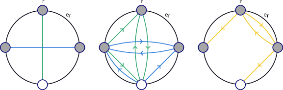
Figure 3: An example of a SRAP instance undergoing preprocessing steps to obtain a complete instance. The leftmost SRAP instance has two undirected links $\ell_{1}$ (green) and $\ell_{2}$ (blue) in $L$. There are no links added in $L_{1}$. The middle picture shows the directed links added in $L_{2}$, where the green arcs are shadows of $\ell_{1}$ and have cost $c(\ell_{1})$, and the blue arcs are shadows of the $\ell_{2}$ with cost $c(\ell_{2})$. Finally, the third picture shows the (undominated) directed links added in $L_{3}$ in yellow. Each of these arcs have cost $c(\ell_{1})+c(\ell_{2})$. The final completed SRAP instance contains all of these links.

4.2 An $R$-special 2-approximate solution

We now proceed with the 2-approximate $R$-special solution for SRAP. First, we make an existential claim about the existence of a 2-approximate directed solution which only touches terminals, then we show that we can find one efficiently.

In the proof of Lemma 4.3, we will first show that there is a 2-approximate directed solution which consists of a collection of directed cycles on nodes of the ring. We will then merge these cycles to obtain a directed solution which is a single directed cycle.

It is helpful to notice that a undirected cycle on nodes $A\subseteq V(H)$ covers the same set of dangerous ring-cuts that a directed cycle on $A$ covers, which is also the same set of dangerous ring-cuts that the hyper-link $A$ covers. This allows us to use Lemma 1.13 to understand when a collection of directed cycles is feasible.

For a node set $A\subseteq V(H)$, denote by $I_{A}\subseteq V(H)$ the nodes in the minimal interval containing $A$ which does not contain $e_{r}$.

Lemma 4.3.

Given an instance of SRAP, suppose the optimal solution has cost OPT. Then there exists a directed solution of cost at most $2\text{OPT}$ whose links consist of a single directed cycle including $r$.

Proof.

Let $(U^{*},F^{*})$ be a full component of the optimal SRAP solution. Then $(U^{*},F^{*})$ is a tree. Starting from an arbitrary vertex in $U^{*}\cap V(H)$, we take an Euler tour of this tree traversing each link exactly twice. This induces an ordering of the ring nodes which are visited during the tour $a_{1},\ldots,a_{k}$, such that the undirected link set $F=\{(a_{1},a_{2}),\ldots,(a_{k-1},a_{k}),(a_{k},a_{1})\}$ has cost at most $2c(F^{*})$ by metric completion.

Now, consider the directed link set $\vec{F}=\{(a_{1},a_{2}),\ldots,(a_{k-1},a_{k}),(a_{k},a_{1})\}$. The cost of $\vec{F}$ is at most $c(F)$ since it consists of shadows of links in $F$. Hence $c(\vec{F})\leq 2c(F^{*})$. Furthermore, since $\vec{F}$ forms a directed cycle on the nodes joined by $F^{*}$, any cut covered by $F^{*}$ is also covered by $\vec{F}$.

Repeating this for each full component in the optimal solution yields a directed solution with cost at most $2\text{OPT}$. Furthermore, this directed solution consists of a collection of directed cycles on the nodes of the ring.

We now exploit the following lemma to obtain a directed solution with cost at most $2\text{OPT}$ consisting of a single directed (not necessarily simple) cycle.

Lemma 4.4 (Cycle Merging Lemma).

Consider a SRAP instance on the ring $H=(V(H),E)$. Let $\vec{F}_{S}$ and $\vec{F}_{A}$ be two directed cycles of links on nodes $S,A\subseteq V(H)$, respectively, where $r\in S$. If $S$ and $A$ are intersecting as hyper-links, then there exists a directed link set $\vec{F}_{S\cup A}$ which forms a directed cycle on $S\cup A$ of cost at most $c(\vec{F}_{S})+c(\vec{F}_{A})$.

Proof.

First observe that if $A\cap S\neq\varnothing$, we simply define $\vec{F}_{S\cup A}=\vec{F}_{S}\cup\vec{F}_{A}$, and the statement of the lemma is satisfied.

So, suppose that $A\cap S=\varnothing$. Denote the cycle links as $\vec{F}_{S}=\{(s_{1},s_{2}),\ldots,(s_{k-1},s_{k}),(s_{k},s_{1})\}$, with $s_{1}=r$, and $\vec{F}_{A}=\{(a_{1},a_{2}),\ldots,(a_{\ell-1},a_{\ell}),(a_{\ell},a_{1})\}$. Consider the interval $I_{A}$ of $A$. Since $S$ and $A$ are intersecting (as hyper-links), and $S$ contains the root $r$ while $r\not\in I_{A}$, it must be the case that the cycle formed by $\vec{F}_{S}$ leaves $I_{A}$ at least once. Let $(s_{i},s_{i+1})\in\vec{F}_{S}$ be a directed link leaving $I_{A}$.

Now consider the interval $I^{*}=I_{\{s_{i},s_{i+1}\}}$. We claim that $\vec{F}_{A}$ leaves $I^{*}$ at least once. Indeed, since $(s_{i},s_{i+1})$ leaves $I_{A}$, some $a\in A$ is in $I^{*}$. But all of $A$ cannot be contained in $I^{*}$, since then $(s_{i},s_{i+1})$ leaving $I_{A}$ would imply that $s_{i}\in A$, contradicting our assumption that $A\cap S=\varnothing$. Let $(a_{j},a_{j+1})\in\vec{F}_{A}$ be a directed link leaving $I^{*}$.

We now define $\vec{F}_{S\cup A}$ to be the directed links along the cycle

$$s_{1},\ldots,s_{i},a_{j+1},a_{j+2},\ldots,a_{j},s_{i+1},\ldots,s_{1}.$$

See Figure 4 for an example. Observe that $(s_{i},a_{j+1})$ is a shortening of $(a_{j},a_{j+1})$ and $(a_{j},s_{i+1})$ is a shortening of $(s_{i},s_{i+1})$. Therefore $c(\vec{F}_{S\cup A})\leq c(\vec{F}_{S})+c(\vec{F}_{A})$ as desired. Moreover, $\vec{F}_{S\cup A}$ forms a cycle on $S\cup A$.

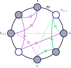
Figure 4: An example of cycle merging, with $\vec{F}_{S}$ in purple and $\vec{F}_{A}$ in green. Note that $(s_{i},s_{i+1})$ leaves the interval $I_{A}$, and $(a_{j},a_{j+1})$ leaves the interval $I_{\{s_{i},s_{i+1}\}}$. Dropping these two links, and adding the shortenings drawn as dotted arcs creates the single cycle $\vec{F}_{S\cup A}$.

∎

We can now use Lemma 4.4 to transform a directed solution that is a collection of directed cycles on ring nodes $A_{1},\ldots,A_{p}$ into a single directed cycle on $A:=\bigcup_{i=1}^{p}A_{i}$. Let $\vec{J}$ denote the directed solution consisting of a collection of directed cycles on the nodes in the ring. Since $r$ is a terminal, it must be contained in some cycle $\vec{F}_{S_{0}}$ on $S_{0}\subseteq V(H)$. We build a new directed solution starting with $\vec{F}_{S_{0}}$ by repeatedly apply Lemma 4.4, cycle merging. In each step, choose a new cycle $\vec{F}_{A}$ from $\vec{J}$ that has not yet been merged and such that $A$ is intersecting with $S_{i}$, and update $\vec{F}_{S_{i}}$ by merging: $\vec{F}_{S_{i+1}}\leftarrow\vec{F}_{S_{i}\cup A}$. If all cycles from $\vec{J}$ can be merged in this way, this yields a single directed cycle. It is feasible, since it is incident to all terminals, and its cost is at most that of $\vec{J}$, which is at most $2\text{OPT}$.

It remains only to show that at every step, if there are un-merged cycles from $\vec{J}$, then one of them is on a set of nodes which is intersecting with $S_{i}$. First, observe that $\vec{F}_{S_{i}}$ is a cycle on all of the nodes belonging to the cycles merged so-far, so it suffices to find some un-merged $\vec{F}_{A}$ in $\vec{J}$ such that $A$ is intersecting with the nodes in one of the cycles merged so-far.

Since $\vec{J}$ is feasible, the corresponding collection of undirected cycles is also feasible. Hence, by Lemma 1.13, the hyper-links on the vertices of the cycles in $\vec{J}$ are connected in the hyper-link intersection graph. Now for any un-merged cycle $\vec{F}_{A^{\prime}}$, look at the path in the hyper-link intersection graph from the hyper-link on $S_{0}$ to the hyper-link on $A^{\prime}$. The first hyper-link along this path corresponding to an un-merged cycle $\vec{F}_{A}$ must be intersecting with a merged cycle, so is intersecting with $S_{i}$. ∎

With the above lemma in hand, and due to our second metric completion step, we can now shortcut over the non-terminals in the cycle to obtain a 2-approximate directed solution which only touches terminals.

Lemma 4.5.

Given an instance of SRAP, if the optimal solution has cost OPT, then there is a directed solution of cost at most $2\text{OPT}$ whose links consist of a single directed cycle with node set $R$.

Proof.

This follows by taking the directed cycle solution $\vec{F}$ from Lemma 4.3 and short-cutting through all non-terminal nodes. Since the third preprocessing step ensures that the directed links are metrically complete, replacing a path of directed links with a single link cannot increase the cost. Hence, the resulting solution has cost at most $c(\vec{F})\leq 2\text{OPT}$. ∎

Having shown that there exists a directed 2-approximate solution to any SRAP instance which is incident only on the terminals $R$, we now proceed to show how to compute one in polynomial time. In particular, we will prove that the optimal such solution can be found efficiently. And moreover, the solution can be assumed to have additional structure.

Recall that the Weighted Ring Augmentation Problem (WRAP) is a special case of SRAP in which all nodes are terminals, and there are no nodes outside of the ring $H$. A directed solution $\vec{F}$ to WRAP is non-shortenable if it is feasible but deleting or strictly shortening any link $f\in\vec{F}$ results in an infeasible solution. Traub and Zenklusen proved that a non-shortenable directed solution to WRAP has a planar arborescence structure, and can be computed in polynomial time.

Lemma 4.6 (Lemma 2.5 in [18]).

A non-shortenable optimal directed solution to the WRAP problem can be found in polynomial time.

Reducing our problem to a WRAP instance and applying the above lemma yields the main theorem of this section:

See 2.1

Proof.

Consider a SRAP instance on the ring $H=(V(H),E)$ with terminals $R\subseteq V(H)$, root $r\in R$, and links $L$. We construct a new ring $H^{\prime}=(R,E^{\prime})$ on the terminals by iteratively replacing each non-terminal node in $V(H)$ with an edge between its two neighbors in $H$. We now create a WRAP instance on $H^{\prime}$ by taking the subset $L^{\prime}$ of links which are directed links incident only to $R$.

We apply Lemma 4.6 (Lemma 2.5 from [18]) to get a non-shortenable optimal directed solution $\vec{F}$ to this WRAP instance. Since Lemma 4.5 guarantees the existence of a directed 2-approximation which only touches terminals, this implies that $c(\vec{F})\leq 2\text{OPT}$.

Now consider $\vec{F}$ as a solution to the SRAP instance on $H$. Since $\vec{F}$ is non-shortenable when viewed as a solution to the WRAP instance on $H^{\prime}$, Theorem 2.6 from [18] shows that it satisfies the three conditions when viewed as a solution to $H$. It remains only to argue that $\vec{F}$ is actually feasible. This is immediate from the arborescence structure of $\vec{F}$: there is a path from $r$ to every terminal. ∎

5 A $(1+\ln{2}+\varepsilon)$-approximation for SRAP

In this section, we describe a polynomial time algorithm for SRAP which achieves an approximation ratio of $(1+\ln{2}+\varepsilon)$. Before writing the algorithm, we comment on a slight departure of our algorithm from the relative greedy algorithm for standard WRAP.

Given any SRAP instance, we may convert it into an equivalent complete instance (see section 4.1). We observe that for any directed link $f=(u,v)$ on the ring, there is a collection of undirected links whose coverage is at least that of $f$, and whose total cost is at most $c(f)$. We call this set $\kappa_{f}$. Indeed, if $f$ is a shadow of an undirected link $\ell$, then we may take $\kappa_{f}=\{\ell\}$. Otherwise, $f$ arises from the metric completion of some directed path of links $(u=s_{0},s_{1}),(s_{1},s_{2}),\ldots,(s_{k-1},s_{k}=v)$. Each of these links in the directed path may themselves be shortenings of undirected links $\{\ell_{1},\ldots,\ell_{k}\}$. In this case, $\kappa_{f}=\{\ell_{1},\ldots,\ell_{k}\}$. Note in particular that $\kappa_{f}$ covers all of the dangerous ring-cuts that $f$ covers, so if $f$ is in some $R$-special solution $\vec{F}_{0}$, then $f\in\text{drop}_{\vec{F}_{0}}(\kappa_{f})$ (see section 6 for a formal definition of drop).

In order to show that our algorithm makes sufficient progress at each step, we must have that the cost of our mixed solution does not ever increase over the course of the algorithm. In the case of WRAP, this is immediate, since any directed link is a shadow of some single undirected link of the same cost, an $\alpha$-thin set. However, in our case, $\kappa_{f}$ may not be $\alpha$-thin, so we explicitly consider this as a separate case in each step of our algorithm. See Algorithm 1.

Algorithm 1 Relative greedy algorithm for SRAP

Input: A complete instance of SRAP with graph $G=(V,E\dot{\cup}L)$, ring $H=(V(H),E)$, terminals $R\subseteq V(H)$ and $c:L\to\mathbb{R}$. Also an $\varepsilon>0$.
Output: A solution $S\subseteq L$ with $c(S)\leq(1+\ln(2)+\varepsilon)\cdot c(\text{OPT})$.

1. Compute a 2-approximate $R$-special directed solution $\vec{F}_{0}$ (Theorem 2.1).

2. Let $\varepsilon^{\prime}:=\frac{\varepsilon/2}{1+\ln 2+\varepsilon/2}$ and $\gamma:=2^{\lceil{1/\varepsilon^{\prime}}\rceil}$.

3. For each $A\subseteq V(H)$ where $|A|\leq\gamma$, compute the cheapest full component joining $A$ and denote the cost by $c_{A}$.

4. Create an instance of $\gamma$-restricted Hyper-SRAP on the ring $H=(V(H),E)$ with hyper-links $\mathcal{L}=\{\ell_{A}:A\subseteq R,|A|\leq\gamma\}$. Set the cost of hyper-link $\ell_{A}$ to be $c_{A}$.

5. Initialize $S_{0}:=\emptyset$

6. Let $\alpha:=4\lceil 4/\varepsilon\rceil$

7. While $\vec{F}_{i}\neq\emptyset$:

   • Increment $i$ by 1.

   • Compute the $\alpha$-thin subset of hyper-links $Z_{i}\subseteq\mathcal{L}$ minimizing $\frac{c(Z_{i})}{c(\text{drop}_{\vec{F}_{0}}(Z_{i})\cap\vec{F}_{i-1})}$.

   • If $\frac{c(Z_{i})}{c(\text{drop}_{\vec{F}_{0}}(Z_{i})\cap\vec{F}_{i-1})}>1$, then update $Z_{i}=\kappa_{f}$ for some $f\in\vec{F}_{i-1}$.

   • Let $S_{i}:=S_{i-1}\cup Z_{i}$ and let $\vec{F}_{i}:=\vec{F}_{i-1}\setminus\text{drop}_{\vec{F}_{0}}(Z_{i})$.

8. Return A SRAP solution with full components corresponding to the hyper-links in $S:=S_{i}$.

The proof of the following theorem follows from a standard analysis of the relative greedy algorithm as in [4], [19], and [18]. We include it here for completeness.

Theorem 5.1.

Algorithm 1 is a $(1+\ln{2}+\varepsilon)$-approximation algorithm for SRAP.

Proof.

First, we note that in each iteration of the algorithm, $|\vec{F}|$ will be reduced by at least 1. The initial value of $|\vec{F}|$ is at most $|R|-1$, so there are polynomially many iterations. By Theorem 8.1, each iteration can be executed in polynomial time. Hence Algorithm 1 runs in polynomial time.

The returned solution $S$ is feasible since the invariant that $S_{i}\cup\vec{F}_{i}$ is a feasible mixed solution is maintained throughout the algorithm.

To complete the proof, we show that $S$ has cost at most $(1+\ln{2}+\varepsilon)\cdot c(\text{OPT})$. Denote by $\text{OPT}_{\gamma}$ the optimal $\gamma$-restricted solution. Apply the decomposition theorem, Theorem 2.3, to $\text{OPT}_{\gamma}$ and the $R$-special solution $\vec{F}_{0}$. It gives a partition $\mathcal{Z}$ of $\text{OPT}_{\gamma}$ into $\alpha$-thin parts, and some $Q\subseteq\vec{F}_{0}$ with $c(Q)\leq\nicefrac{{\varepsilon}}{{4}}\cdot c(\vec{F}_{0})\leq\nicefrac{{\varepsilon}}{{2}}\cdot c(\text{OPT})$. Then observe that

$$\frac{c(Z_{i})}{c(\text{drop}_{\vec{F}_{0}}(Z_{i})\cap\vec{F}_{i-1})}\leq\min_{Z\in\mathcal{Z}}\frac{c(Z)}{c(\text{drop}_{\vec{F}_{0}}(Z)\cap\vec{F}_{i-1})}\leq\frac{\sum_{Z\in\mathcal{Z}}c(Z)}{\sum_{Z\in\mathcal{Z}}c(\text{drop}_{\vec{F}_{0}}(Z)\cap\vec{F}_{i-1})}\leq\frac{c(\text{OPT}_{\gamma})}{c(\vec{F}_{i-1})-c(Q)},$$

where the first inequality is by the choice of $Z_{i}$ in the algorithm, and the second and third follow from the statement of Theorem 2.3. Since $f\in\text{drop}_{\vec{F}_{0}}(\kappa_{f})$, our choice of $Z_{i}$ implies that, $\nicefrac{{c(Z_{i})}}{{c(\text{drop}_{\vec{F}_{0}}(Z_{i})\cap\vec{F}_{i})}}\leq 1$. Therefore, since $\text{drop}_{\vec{F}_{0}}(Z_{i})\cap\vec{F}_{i-1}=\vec{F}_{i-1}\setminus\vec{F}_{i}$, we have

$$c(Z_{i})\leq\min\left\{1,\frac{c(\text{OPT}_{\gamma})}{c(\vec{F}_{i})-c(Q)}\right\}\cdot c(\vec{F}_{i-1}\setminus\vec{F}_{i})\leq\int_{c(\vec{F}_{i})}^{c(\vec{F}_{i-1})}\min\left\{1,\frac{c(\text{OPT}_{\gamma})}{x-c(Q)}\right\}\,dx.$$

Finally, sum over all iterations of the algorithm to get the cost of the output $S$:

$$c(S) =\sum_{i}c(Z_{i})$$

$$\leq\int_{0}^{c(\vec{F}_{0})}\min\left\{1,\frac{c(\text{OPT}_{\gamma})}{x-c(Q)}\right\}\,dx$$

$$=\int_{0}^{c(\text{OPT}_{\gamma})+c(Q)}1\,dx+\int_{c(\text{OPT}_{\gamma})+c(Q)}^{c(\vec{F}_{0})}\frac{c(\text{OPT}_{\gamma})}{x-c(Q)}\,dx$$

$$\leq\left(1+\frac{\varepsilon}{2}\right)\cdot c(\text{OPT}_{\gamma})+\ln\left(\frac{c(\vec{F}_{0})-c(Q)}{c(\text{OPT}_{\gamma})}\right)\cdot c(\text{OPT}_{\gamma})$$

$$\leq\left(1+\ln(2)+\frac{\varepsilon}{2}\right)\cdot c(\text{OPT}_{\gamma})$$

And applying Lemma 1.16 for our choice of $\varepsilon^{\prime}$ and $\gamma$ from the algorithm, we have $c(\text{OPT}_{\gamma})\leq(1+\varepsilon^{\prime})\cdot c(\text{OPT})$. Hence, we get the desired bound

$$c(S)\leq\left(1+\ln(2)+\frac{\varepsilon}{2}\right)\cdot(1+\varepsilon^{\prime})\cdot c(\text{OPT})=\left(1+\ln(2)+\varepsilon\right)\cdot c(\text{OPT}).\qed$$

6 Dropping Directed Links

The main reason that we work with structured $R$-special directed solutions to SRAP is that it allows us to cleanly characterize when a directed link can be dropped after a collection of hyper-links are added to the solution. In this section, we recall the properties of an $R$-special directed solution and use them give such a characterization.

Given an instance of Hyper-SRAP we can use the root $r$ and root-edge $e_{r}$ to define a notion of right and left along the ring. In particular, we imagine deleting the edge $e_{r}$ from the ring and consider the root to be the left-most node on the remaining path. The other node incident to $e_{r}$ is the right-most node in the ring.

Consider a $R$-special directed solution $\vec{F}$ for the SRAP problem. Recall that $\vec{F}$ has the following properties:

1. $\vec{F}$ is only incident on terminals $R$.

2. $(R,\vec{F})$ is an $r$-out arborescence.

3. $(R,\vec{F})$ is planar when $V(H)$ is embedded as a circle in the plane.

4. For any $v\in R$, no two directed links in $\delta^{+}_{\vec{F}}(v)$ go in the same direction along the ring.

Given an $R$-special directed SRAP solution $\vec{F}$, we associate to each cut $C\in\mathcal{C}$ a single link which is responsible for covering it, as in [18]. In particular, an arc $\ell=(u,v)\in\vec{F}$ is responsible for covering a cut $C\in\mathcal{C}$ if $\ell$ enters $C$ and there is no other arc on the unique $r$–$u$ path in $(R,\vec{F})$ which enters $C$. We denote the set of cuts for which a link $\ell\in\vec{F}$ is responsible by $\mathcal{R}_{\vec{F}}(\ell)$. Notice that $\mathcal{R}_{\vec{F}}(\ell)\neq\emptyset$ for all $\ell\in\vec{F}$, since if some directed link were not responsible for any cuts, then it could be deleted without affecting the feasibility of $\vec{F}$, but this is not true of any arc in an $R$-special directed solution.

We will show that every ring-dangerous cut $C\in\mathcal{C}$ has exactly one directed link responsible for it in an $R$-special solution $\vec{F}$. First we will need the following lemma which follows from the properties of $\vec{F}$.

Lemma 6.1.

Let $\vec{F}$ be an $R$-special directed solution for SRAP.

1. For any $v\in R$, the set of descendants of $v$ in $(R,\vec{F})$ is of the form $R\cap I$ for some ring interval $I\subseteq V(H)$.

2. For $v_{1},v_{2}\in R$, the least common ancestor of $v_{1}$ and $v_{2}$ in $(R,\vec{F})$ lies between $v_{1}$ and $v_{2}$.

This is an analogue to Lemma 4.8 from [18]. In fact, this lemma follows immediately from Lemma 4.8 from [18] by simply removing the Steiner nodes in the ring and viewing $\vec{F}$ as an $R$-special solution on a ring with only the terminals $R$ (c.f. the proof of Theorem 2.1).

Lemma 6.2.

For each cut $C\in\mathcal{C}$, there is exactly one directed link $\ell\in\vec{F}$ responsible for it.

Proof.

A cut $C\in\mathcal{C}$ clearly has at least one link responsible for it, since $\vec{F}$ enters all such cuts. On the other hand, no two links can both be responsible for $C$. This is because $C$ is an interval, so if $(u_{1},v_{1})\neq(u_{2},v_{2})$ are both responsible for $C$, then the least common ancestor $v$ of $v_{1}$ and $v_{2}$ is in $C$, by Lemma 6.1ii. Since $r\not\in C$, there must be some link in the $r$–$v$ path in $(R,\vec{F})$ (and hence also on the $r$–$v_{1}$ path) entering $C$, contradicting that $(u_{1},v_{1})$ is responsible for $C$. ∎

We can now define when a directed link will be dropped from an $R$-special directed solution $\vec{F}$. In particular, if a collection of hyper-links $K$ is added to the solution, then we will drop a directed link if and only if all cuts it is responsible for are covered by the hyper-links in $K$. Let $\delta_{K}(C)$ be the set of hyper-links in $K$ which cover $C\in\mathcal{C}$.

Formally, denote

$$\text{drop}_{\vec{F}}(K)=\{f\in\vec{F}:|\delta_{K}(C)|\geq 1\text{ for all }C\in\mathcal{R}_{\vec{F}}(f)\}.$$

With this definition, if a collection of hyper-links $K$ is added to an $R$-special directed solution $\vec{F}$ to SRAP, and $\text{drop}_{\vec{F}}(K)$ is removed, then the solution remains feasible as a mixed SRAP solution.

Our ultimate goal of this section is an alternate characterization of the set $\text{drop}_{\vec{F}}(K)$. For this, we will use the notion of the hyper-link intersection graph. Recall that a pair of hyper-links $\ell_{1}$ and $\ell_{2}$ are intersecting if they share a vertex or there is a vertex in $\ell$ between two vertices in $\ell^{\prime}$ and a vertex of $\ell^{\prime}$ lies between two vertices of $\ell$.

Given an instance of Hyper-SRAP with ring $H=(V(H),E)$ and hyper-links $\mathcal{L}$, we define the hyper-link intersection graph $\Gamma$ as follows. For each hyper-link $\ell\in\mathcal{L}$ there is a node $v_{\ell}$. Two nodes $v_{\ell_{1}}$ and $v_{\ell_{2}}$ are adjacent in the hyper-link intersection graph if and only if $\ell_{1}$ and $\ell_{2}$ are intersecting hyper-links. For $K\subseteq\mathcal{L}$, $\Gamma(K)$ is the hyper-link intersection graph restricted to the hyper-links in $K$.

The following lemma and its proof are similar to the analogous statements for standard links (Lemma 5.4 in [18]).

Lemma 6.3.

Let $K\subseteq\mathcal{L}$ be a collection of hyper-links, and $C\in\mathcal{C}$ a dangerous ring-cut. Then $\delta_{K}(C)\neq\varnothing$ if and only if there is a path in $\Gamma(K)$ from a hyper-link containing some $v\in C$ to a hyper-link containing some $w\not\in C$.

Proof.

If $\delta_{K}(C)\neq\varnothing$, then clearly such a path in $\Gamma(K)$ exists. In particular, any single hyper-link in $\delta_{K}(C)$ forms a path. Conversely, suppose such a path exists in $\Gamma(K)$, but that $\delta_{K}(C)=\varnothing$ for contradiction. That is, any hyper-link in $K$ is either fully contained $C$ or fully contained in $V(H)\setminus C$. Since the path starts with a hyper-link containing $v\in C$, and ends with one containing $w\not\in C$, the path must contain some pair of intersecting hyper-links $\ell_{1}$ and $\ell_{2}$ with $\ell_{1}$ contained in $C$, while $\ell_{2}$ is contained in $V(H)\setminus C$. Hence, clearly $\ell_{1}$ and $\ell_{2}$ do not share a vertex. Furthermore, since $C$ is an interval, any vertex lying between two vertices in $\ell_{1}$ must also lie in $C$, and hence not in $\ell_{2}$. This contradicts that $\ell_{1}$ and $\ell_{2}$ are intersecting. ∎

Lemma 6.3 yields Lemma 1.13 as an immediate corollary, but we will not need Lemma 1.13 in this section.

The notions of $v$-bad and $v$-good were used in [18], but the definitions need to be modified for our setting.

Definition 6.4.

Let $v\in R$ and consider the maximal interval $I_{v}\subseteq V(H)$ containing $v$ such that $I_{v}$ does not contain a terminal which is a non-descendant of $v$ in $(R,\vec{F})$. We say that the nodes in $I_{v}$ are $\boldsymbol{v}$-bad, and all nodes in $V(H)\setminus I_{v}$ are $\boldsymbol{v}$-good.

Observe that by Lemma 6.1i, the interval of $v$-bad nodes actually contains all descendants of $v$ (but may also contain some Steiner nodes in the ring).

The following lemmas are analogous to Lemmas 5.6 and 2.10, respectively, in [18]. The proofs are similar, but we include them here as our definitions of $v$-good and $v$-bad have changed.

Lemma 6.5.

A directed link $(u,v)\in\vec{F}$ is responsible for a cut $C\in\mathcal{C}$ if and only if $v\in C$ and all of the nodes in $C$ are $v$-bad.

Proof.

If $v\in C$ and all nodes of $C$ are $v$-bad, then $C\cap R$ contains only descendants of $v$. In particular, $u\not\in C$, so $(u,v)$ enters $C$, and no other link on the $r$–$v$ path in $\vec{F}$ can enter $C$.

Conversely, if $(u,v)$ is responsible for cut $C$, then it enters $C$, so $v\in C$. Moreover, for every $t\in C\cap R$, the $r$–$t$ path in $\vec{F}$ must have a link entering $C$. By Lemma 6.2 we know that $(u,v)$ is the only link responsible for $C$, so every such $t$ must be a descendant of $v$. That is, $C\cap R$ are all descendants of $v$, and in particular, $C$ contains no terminals which are non-descendants of $v$. Hence, since $C$ is an interval, it is contained in the maximal interval containing no terminal non-descendants of $v$, which is precisely the set of $v$-bad nodes. ∎

This yields the main result of this section, which provides a characterization of when a directed link $(u,v)$ can be dropped, namely when $v$ is connected to a $v$-good vertex through the hyper-link intersection graph. This is the criterion we will work with in section 7.

Lemma 6.6.

For a collection of hyper-links $K$, a directed link $(u,v)$ is in $\text{drop}_{\vec{F}}(K)$ if and only if $\Gamma(K)$ contains a path from a hyper-link containing $v$ to a hyper-link containing a $v$-good vertex $w$.

Proof.

First suppose that there is such a path in $\Gamma(K)$. Then any cut $C\in\mathcal{R}_{\vec{F}}((u,v))$ for which $(u,v)$ is responsible cannot contain $w$, since by Lemma 6.5 it only contains $v$-bad nodes. Hence, by Lemma 6.3, we have that $\delta_{K}(C)\neq\varnothing$.

Conversely, if $v$ is not connected to a $v$-good vertex by $K$ in the hyper-link intersection graph, then consider the set $K_{v}\subseteq V(H)$ of nodes reachable from $v$ via the hyper-link intersection graph of $K$. Let $I_{K_{v}}$ be the interval of these nodes. Then $I_{K_{v}}\in\mathcal{C}$, since $v\in I_{K_{v}}$, $r\not\in I_{K_{v}}$ (since $r$ is $v$-good) and it is a 2-cut. Moreover, since $K_{v}$ are all $v$-bad, then $I_{K_{v}}$ are as well. By Lemma 6.5, this implies that $(u,v)$ is responsible for the cut $I_{K_{v}}$. We finish the proof by arguing that $K$ does not cover $I_{K_{v}}$, implying that $(u,v)\not\in\text{drop}_{\vec{F}}(K)$. This is clear from the definition of the hyper-link intersection graph: if some hyperlink in $K$ covers $I_{K_{v}}$, then it must be intersecting with a hyperlink reachable from $v$ in the hyper-link intersection graph, thus contradicting that $K_{v}$ are all of the nodes reachable from $v$ in the hyper-link intersection graph of $K$. ∎

7 The Decomposition Theorem for Hyper-SRAP

In this section, we prove the following theorem.

See 2.3

We follow the approach in [18] which proves the result when all hyper-links have size 2 and $R=V(H)$. We will first partition the hyper-links in $S$ into a collections of festoons whose spans form a laminar family. We will then construct a dependency graph whose nodes correspond to festoons, which will allow us to partition the links of $S$ into the desired $\alpha$-thin pieces. In the general hyper-link setting, the festoons are composed of hyper-links rather than links of size 2.

We begin by defining festoons in the context of hyper-links. The interval of a hyper-link $\ell$ is denoted $I_{\ell}$ and is the set of vertices in the interval between the leftmost vertex and the rightmost vertex of $\ell$. We say that hyper-links $\ell$ and $\ell^{\prime}$ are crossing if their intervals intersect and neither is a subset of the other. Recall that two hyper-links are intersecting if they share a vertex, or there is a vertex in $\ell$ between two vertices in $\ell^{\prime}$ and a vertex of $\ell^{\prime}$ lies between two vertices of $\ell$ (when the vertices are viewed in the left to right order along the ring). Notice that if two hyper-links are crossing, then they also are intersecting.

Definition 7.1.

A festoon is a set of hyper-links $X\subseteq\mathcal{L}$ which can be ordered $\ell_{1},\ldots,\ell_{p}$ such that $\ell_{i}$ and $\ell_{i+1}$ are crossing for $i\in\{1,\ldots,p-1\}$ and $I_{\ell_{i}}$ and $I_{\ell_{j}}$ are disjoint unless $|i-j|=1$.

Notice that whether a set of hyper-links is a festoon only depends on their hyper-link intervals. Let $\mathcal{C}^{\prime}=\{C\subseteq V(H):|\delta_{E}(C)|=2,r\not\in C\}$ be the family of minimum cuts of the ring $H$. One of the key properties of festoons is that no minimum cut is covered by more than 4 hyper-links in a festoon.

Lemma 7.2.

Let $X$ be a festoon and $C\in\mathcal{C}^{\prime}$. Then $|\{\ell\in X:\ell\text{ covers }C\}|\leq 4$.

Proof.

Suppose $X={\ell_{1},\ldots,\ell_{p}}$ is a festoon of hyper-links and $C\in\mathcal{C}^{\prime}$. Then $C$ is an interval between vertices say $u$ and $v$ in $V(H)$, where $u$ is the left endpoint of $C$ and $v$ is the right endpoint.

We will show that there are at most two hyper-links in $\delta_{X}(C)$ which contain vertices to the left of $u$. A symmetric argument shows that there can be at most two hyper-links in $\delta_{X}(C)$ containing a vertex to the right of $v$. Together, these imply that there are at most 4 hyper-links in $\delta_{X}(C)$.

Suppose there are 3 hyper-links covering $C$ which contain vertices to to the left of $u$. Since they cover $C$, each of these hyper-links must also contain some vertex in $C$. Thus, their hyper-link intervals all contain the vertex $u$. But this is impossible, as the definition of festoons requires that $I_{\ell_{i}}$ and $I_{\ell_{j}}$ are disjoint unless $|i-j|=1$. ∎

Definition 7.3 ($\alpha$-thin set of hyper-links).

A set of hyper-links $K$ is $\alpha$-thin if there exists a maximal laminar subfamily $\mathcal{D}$ of $\mathcal{C}^{\prime}$ such that for every cut $C\in\mathcal{D}$, we have $|\{\ell\in K:\ell\text{ covers }C\}|\leq\alpha$.

Given a festoon $X$, let $I_{X}$ denote the festoon interval which is the interval from the left-most vertex in the festoon to the right-most. We can partition $S$ into a collection of festoons $\mathcal{X}$, so that the festoon intervals form a laminar family. To do this, we iteratively construct the partition by choosing a festoon with the largest interval in each iteration and adding it to the partition. We now prove that if the set $S$ is partitioned in this way, it yields a partition $\mathcal{X}$ such that the set of festoon intervals form a laminar family.

Lemma 7.4.

The festoon intervals $\{I_{X}:X\in\mathcal{X}\}$ form a laminar family.

Proof.

Suppose that $X,Y\in\mathcal{X}$ are such that $I_{X}$ and $I_{Y}$ cross. We also assume without loss of generality that $X$ was added the festoon family before $Y$ was.

Let $\ell_{1},\ldots,\ell_{p}$ be the hyper-links in the festoon $X$, numbered according to the festoon order. We will assume $X$ is to the left of $Y$. Since they cross, there is some hyper-link in $Y$ whose left endpoint is in $I_{X}$. But then this hyper-link would have been included in $X$ to form a longer interval. ∎

Given the laminar structure of the festoon intervals, we can define a partial order on the festoons in $\mathcal{X}$. In particular, we will say that $X\prec Y$ if $I_{X}\subseteq I_{Y}$.

Definition 7.5.

We say that two festoons $X$ and $Y$ are tangled if some hyper-link in $X$ is intersecting with some hyper-link of $Y$.

Suppose that $X_{1},\ldots,X_{p}$ is a sequence of festoons such that $X_{1}$ contains a vertex $v\in R\setminus r$, $X_{i}$ and $X_{j}$ are tangled iff $|i-j|=1$, and $X_{p}$ contains a $v$-good vertex, but no festoons $X_{i}$ for $i<p$ contain a $v$-good vertex. Then by Lemma 6.6, $\{X_{1},\ldots,X_{p}\}$ is a minimal collection of festoons such that the directed link $(u,v)\in\vec{F}$ can be dropped. We will choose for each $v\in R$, a minimal collection of festoons $\mathcal{X}_{v}=\{X_{1},\ldots,X_{p}\}$ as above so that $|I_{X_{p}}|$ is minimized. This will allow us to construct the dependency graph with the desired properties.

We now turn to defining the dependency graph $(\mathcal{X},A)$. It will have a vertex for each festoon in $\mathcal{X}$, and its arcs are obtained by inserting for each directed link $(u,v)\in\vec{F}$ a directed path corresponding to a minimal set of festoons as above. Formally, for each $v\in R\setminus r$, there will be a directed path $P_{v}$ consisting of the festoons in $\mathcal{X}_{v}$ where $(X_{i},X_{i-1})\in A$ for $i\in\{2,\ldots p\}$.

It will be helpful to consider a subgraph of the dependency graph which is constructed only from paths $P_{v}$ where $v\in U$ for some set of terminals $U\subseteq R\setminus r$. This is called the $U$-dependency graph.

We will use that the dependency graph is a branching, which follows from the minimality in its construction and the partial order defined on festoons. Clearly, this implies that the $U$-dependency graph is also a branching for any $U\subseteq R\setminus r$.

Lemma 7.6.

The dependency graph $(\mathcal{X},A)$ is a branching. That is, the in-degree of every node $X\in\mathcal{X}$ is at most 1 and it contains no cycles.

Proof.

Since $(X,Y)\in A$ implies $Y\prec X$, it is clear that $(\mathcal{X},A)$ contains no directed cycles. We now show that each festoon $X$ has in-degree at most 1. Suppose for the sake of contradiction that $(Y,X)\in A$ and $(Z,X)\in A$ where $Y\neq Z$. Since the arcs in $A$ arise from a collection of directed paths, it must be the case that $(Y,X)\in P_{v}$ and $(Z,X)\in P_{w}$ for distinct vertices $v,w\in R\setminus r$.

We will use the following key property, used in [18], which continues to hold in our setting: for any pair of terminals $v,w\in R\setminus r$, either $w$ is $v$-good or $v$ is $w$-good. Hence, we assume without loss of generality that $w$ is $v$-good.

Since $(Z,X)\in P_{w}$, we have that $w$ is contained in the festoon interval $I_{X}$ of $X$. Since the $v$-good vertices form an interval, $X$ must contain a hyper-link which contains a $v$-good vertex. But by Lemma 6.6, this means that $Y$ is not necessary for a directed link entering $v$ to be dropped, contradicting $(Y,X)\in P_{v}$. ∎

We can bound the thinness of the components of the dependency graph with the following lemmas, which are direct extensions of analogous lemmas in [18]. Let $\alpha$ be some positive integer, and $U\subseteq R\setminus r$.

Lemma 7.7.

If $\mathcal{X}^{\prime}$ is a connected component of the $U$-dependency graph and the set

$$\{Z\in\mathcal{X}^{\prime}:X\preceq Z,\text{ }X\text{ and }Z\text{ are tangled}\}$$

has cardinality at most $\alpha$ for every festoon $X\in\mathcal{X}^{\prime}$, then $\mathcal{X}^{\prime}$ is $4(\alpha+1)$-thin.

Proof.

The proof is the same as the proof of Lemma 7.16 in [18]. Note that Lemma 7.8 in [18] holds for festoons of hyper-links as well as standard festoons. ∎

Lemma 7.8.

Suppose $X$ and $Y$ are festoons in the same connected component of the $U$-dependency graph. If $X$ and $Y$ are tangled, then they have an ancestor-descendant relationship in the $U$-dependency graph.

Proof.

Again, the proof is a direct extension of Lemma 7.17 in [18]. ∎

Lemma 7.9.

Let $(\mathcal{X}^{\prime},A^{\prime})$ be a connected component of the $U$-dependency graph. If

$$|\{u\in V:P\cap P_{u}\neq\emptyset\}|\leq\alpha$$

for every directed path $P\subseteq A^{\prime}$ then the collection of links which are contained in festoons of $\mathcal{X}^{\prime}$ is $4(\alpha+1)$-thin.

Proof.

First, notice that for every $X\in\mathcal{X}$, there are at most $\alpha$ festoons in $\mathcal{X}^{\prime}$ which are at least $X$ in the partial ordering. This is because $X$ can be tangled with at most one festoon from each $P_{u}$, which follows from minimality as well as Lemma 7.8. Hence, by Lemma 7.7, $\mathcal{X}^{\prime}$ is $4(\alpha+1)$-thin as desired. ∎

Having shown that the dependency graph is a branching, the property given in Lemma 7.9 is enough to replicate the same argument which was introduced by Traub and Zenklusen in [19] for the Weighted Tree Augmentation Problem to prove the decomposition theorem. We break the dependency graph up into pieces, such that each corresponds to a collection of hyper-links which is $\alpha$-thin, while only destroying a small fraction of the sets $P_{u}$. We reproduce the proof below.

See 2.3

Proof.

Let $q:=\lceil\frac{1}{\varepsilon}\rceil$. We will construct an arc labeling for each connected component $(\mathcal{X}^{\prime},A^{\prime})$ of the $(R\setminus r)$-dependency graph $(\mathcal{X},A)$, which is a branching by Lemma 7.6. The arcs in the same set $P_{u}$ will receive the same label.

We define the labeling inductively as follows. For each directed path $P_{u}$ which begins at the root of the arborescence $(\mathcal{X}^{\prime},A^{\prime})$, we set the labels of the arcs in this path to be 0. For a directed path $P_{u}$ which begins at a node $X$ which is not the root, we set the label of the arcs in $P_{u}$ to be $j+1$, where $j$ is the label of the unique arc entering $X$. We perform the labeling in this fashion for each connected component of the dependency graph to obtain a labeling of all arcs in $A$

Now, let $Q_{i}\subseteq\vec{F}$ be the set of directed links $(u,v)$ such that $P_{v}$ received label $i$, where $i\in\{0,\ldots,q-1\}$. This is a partition of $\vec{F}$ into $q$ parts. Hence, the average cost of the sets $Q_{i}$ is $c(\vec{F})/q$, implying that the cheapest set among $Q_{0},\ldots,Q_{q-1}$ has cost at most $c(\vec{F})/q$. Let this cheapest part be denoted by $Q\subseteq\vec{F}$.

We define $U\subseteq R$ to be those terminals which are not entered by a directed link in $Q$, and consider the $U$-dependency graph. The $U$-dependency graph is obtained by deleting from $(\mathcal{X},A)$ all arcs with label $i$ for some $i\in\{0,\ldots,q-1\}$. Hence, each of its connected components satisfies the hypothesis of Lemma 7.9 where $\alpha=q-1$, implying that the set of hyper-links in the festoons of each component is $4q$-thin. This yields our partition of the hyper-links of $S$ into parts where each part is $4\lceil\frac{1}{\varepsilon}\rceil$-thin.

Finally, for each directed link $(u,v)\in\vec{F}\setminus Q$ there is some connected component of the $U$-dependency graph which contains all the arcs in $P_{v}$. Hence, $(u,v)$ is droppable by adding all the hyper-links in the festoons of this component. Since, $c(Q)\leq\varepsilon\cdot c(\vec{F})$, we have the desired property. ∎

8 Dynamic Programming to find the best $\alpha$-thin component

In this section, we prove that, given an $R$-special directed solution $\vec{F}_{0}$, and a subset $\vec{F}\subseteq\vec{F}_{0}$, the $\alpha$-thin collection of $\gamma$-restricted hyper-links $K$ which minimizes the ratio

$$\frac{c(K)}{c(\text{drop}_{\vec{F}}(K)\cap\vec{F}_{0})}$$

can be found in polynomial time.

As is now standard following the results of [19][18][17], we will focus on maximizing $\text{slack}_{\rho}(K)$ defined as

$$\text{slack}_{\rho}(K):=\rho\cdot c(\text{drop}_{\vec{F}}(K)\cap\vec{F}_{0})-c(K).$$

Notice that deciding whether the ratio $\frac{c(K)}{c(\text{drop}_{\vec{F}}(K))}$ is smaller than a fixed $\rho^{*}$ is equivalent to deciding whether $\text{slack}_{\rho^{*}}(K)$ is greater than 0. Thus, if we can efficiently find a maximizer of the slack function for any given $\rho$, then we can use binary search to obtain our desired result.

It will be convenient for the results in section 9 to prove a more general result allowing different cost functions on the two terms of the slack function.

Theorem 8.1.

Given an instance of SRAP, let $\vec{F}_{0}$ be an $R$-special directed solution. Let $\tilde{c}:\vec{F}_{0}\to\mathbb{R}_{\geq 0}$ be a cost function on $\vec{F}_{0}$. Then a maximizer of $\tilde{c}(\text{drop}_{\vec{F}_{0}}(K))-c(K)$ over all $\alpha$-thin subsets of $\gamma$-restricted hyper-links can be computed in polynomial time.

Given Theorem 8.1, we can maximize $\text{slack}_{\rho}$ by setting $\tilde{c}(\ell)=\rho\cdot c(\ell)$ for $\ell\in\vec{F}\cap\vec{F}_{0}$ and 0 otherwise. We will prove the above theorem by dynamic programming.

Traub and Zenklusen prove this optimization theorem for the WRAP problem in [18]. The proof in our setting is an extension of their methods. The key differences in our context are twofold. First, we are working with an $R$-special directed solution $\vec{F}_{0}$ which is incident only on the terminals $R$, whereas in WRAP, the arborescence contains all the nodes of the ring. Secondly, we must extend their techniques to hyper-links, rather than standard undirected links containing pairs of vertices of the ring.

To handle this, we will add artificial links to the $R$-special solution $\vec{F}_{0}$ to obtain a $V(H)$-special solution $\vec{F}^{\prime}$, which allows us to extend the least common ancestor function to all subsets of ring nodes. This allows us to leverage Lemma 8.4, which is the analogue of Lemma 2.11 in [18], and is crucial in computing new table entries from already computed ones. Finally, we exploit the fact that we are only working with hyper-links of size at most $\gamma$, implying that there are polynomially many hyper-links available.

To state Lemma 8.4, we will need to extend the notion of the least common ancestor to a set of ring nodes, some of which may not be involved in the arborescence $\vec{F}_{0}$. We first prove some useful properties of $v$-bad intervals. Recall that for a terminal $v\in R$, its $v$-bad interval is the maximal interval containing $v$ which does not include a terminal non-descendant of $v$ in $\vec{F}_{0}$. We show that this collection of intervals is a laminar family.

Lemma 8.2.

Suppose $\vec{F}_{0}$ is an $R$-special solution, and let $I_{v}\subseteq V(H)$ denote the $v$-bad interval. Then the family of all $v$-bad intervals $\mathcal{F}=\{I_{v}:v\in R\}$ is laminar.

Proof.

Consider two terminals $u$ and $v$ with $u$-bad interval $I_{u}$ and $v$-bad interval $I_{v}$. By Lemma 6.1ii, the least common ancestor (in $\vec{F}_{0}$) $w$ of $u$ and $v$, lies between them. If $w$ is not $u$ or $v$, then it is a non-descendant of both of them, so neither $I_{u}$ nor $I_{v}$ can contain $w$. Since $u\in I_{u}$ and $v\in I_{v}$, these intervals do not intersect.

Otherwise, $w$ is equal to either $u$ or $v$; suppose $w=u$ without loss of generality. But then all non-descendants of $u$ are non-descendants of $v$, so $I_{v}\subseteq I_{u}$. Thus, the family is laminar. ∎

We now describe how we add artificial directed links to the $R$-special solution $\vec{F}_{0}$ to obtain a $V(H)$-special solution $\vec{F}^{\prime}$. We will then use $\vec{F}^{\prime}$ to define a notion of least common ancestor in $\vec{F}_{0}$ that is defined for any subset of ring nodes.

For each terminal $v\in R$, define the set of nodes $S_{v}\subseteq V(H)$ to consist of all nodes $u$ such that $I_{v}$ is the minimal interval of $\mathcal{F}$ which contains $u$. Notice that $S_{v}$ is an interval containing exactly one terminal, namely $v$, and potentially Steiner nodes to the left and right of $v$. Suppose $S_{v}=S^{L}_{v}\cup S^{R}_{v}\cup\{v\}$ where $S^{L}_{v}$ and $S^{R}_{v}$ are the (possibly empty) sets of Steiner nodes in $S_{v}$ to the right and left of $v$ respectively. Suppose $S^{L}_{v}=\{s^{L}_{0},\ldots,s^{L}_{k}\}$ ordered right to left along the ring, and $S^{R}_{v}=\{s^{R}_{0},\ldots,s^{R}_{m}\}$ ordered left to right along the ring. We now add the set of artificial directed links $\{(v,s^{L}_{0}),(s^{L}_{0},s^{L}_{1}),\ldots,(s^{L}_{k-1},s^{L}_{k})\}\cup\{(v,s^{R}_{0}),(s^{R}_{0},s^{R}_{1}),\ldots,(s^{R}_{m-1},s^{R}_{m})\}$. See Figure 5.

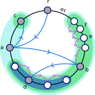
Figure 5: An example of an $R$-special solution with $R=\{r,a,b,c,d\}$ and its extension to an artificial $V(H)$-special solution. The artificial links are purple. The $r$-bad interval is always $V(H)$. The $a$-bad interval is shown in cyan. The $b$-bad and $c$-bad intervals are green, and the $d$-bad interval is dark blue. Note that $\overline{\text{lca}}(\{e,f\})=e$ and $\overline{\text{lca}}(\{e,f,d\})=b$.

When these artificial links are added to $\vec{F}_{0}$, we obtain an associated $V(H)$-special solution $\vec{F}^{\prime}$. Observe that for a terminal $v$, the set of descendants of $v$ in $\vec{F}^{\prime}$ (including $v$ itself) is exactly its $v$-bad interval $I_{v}$.

Definition 8.3 (Extended Least Common Ancestor Function).

Suppose $\vec{F}_{0}$ is an $R$-special solution and $A\subseteq V(H)$. Then the least common ancestor of $A$ with respect to $\vec{F}_{0}$ is

$$\overline{\text{lca}}(A):=\text{lca}_{\vec{F}^{\prime}}(A),$$

where $\text{lca}_{\vec{F}^{\prime}}(A)$ is the least common ancestor of $A$ in the artificial solution $\vec{F}^{\prime}$.

Notice that the above definition coincides with the standard least common ancestor function with respect to $\vec{F}_{0}$ on sets $A$ which consist only of terminals.

Now we can state the key Lemma 8.4. For a set of hyper-links $S$, let $V(S):=\bigcup_{\ell\in S}\ell$.

Lemma 8.4.

If $\vec{F}_{0}$ is an $R$-special directed solution to SRAP and $S\subseteq\mathcal{L}$ is a collection of hyper-links which form a connected component in the hyper-link intersection graph, then

$$\text{drop}_{\vec{F}_{0}}(S)=\Big{(}\bigcup_{v\in V(S)}\delta_{\vec{F}_{0}}^{-}(v)\Big{)}\setminus\delta_{\vec{F}_{0}}^{-}(\overline{\text{lca}}(V(S))).$$

Proof.

First, observe that if $V(S)\cap R=\varnothing$, then both sets in the lemma statement are empty, and the lemma is true. So assume that $V(S)$ contains some terminal.

Since $\delta^{-}_{\vec{F}_{0}}(v)=\emptyset$ whenever $v\not\in R$, we consider some vertex $v\in V(S)\cap R$. Suppose that $v\neq\overline{\text{lca}}(V(S))$. Since $v\in V(S)$, there must be some vertex $u$ in $V(S)$ which is not a descendant of $v$ with respect to $\vec{F}^{\prime}$. Since the set of descendants of $v$ in $\vec{F}^{\prime}$ is exactly the $v$-bad interval $I_{v}$, we have that $u$ is a $v$-good vertex. Thus, by Lemma 6.6, we have that $\delta_{\vec{F}_{0}}^{-}(v)\in\text{drop}_{\vec{F}_{0}}(S)$, since $S$ connects $v$ to a $v$-good vertex via the hyper-link intersection graph.

On the other hand, if $v=\overline{\text{lca}}(V(S))$, then all other vertices in $V(S)$ are descendants of $v$ in $\vec{F}^{\prime}$. Again, the set of descendants of $v$ in $\vec{F}^{\prime}$ is its $v$-bad interval $I_{v}$, so all vertices in $V(S)$ are $v$-bad, and so by Lemma 6.6, $\delta_{\vec{F}_{0}}^{-}(v)$ is not contained in $\text{drop}_{\vec{F}_{0}}(S)$. ∎

In the following, we will build up a solution by considering subproblems defined on intervals of the ring. As such we need a definition of a hyper-link set which is an $\alpha$-thin with respect to an interval $C\subseteq V(H)$.

For a ring $H=(V(H),E)$, let the set of 2-cuts not containing the root be denoted by $\mathcal{C}^{\prime}:=\{C\subseteq V(H):|\delta_{E}(C)|=2,r\not\in C\}$. Recall that a collection of hyper-links $K$ is $\alpha$-thin if there exists a maximal laminar subfamily $\mathcal{D}$ of $\mathcal{C^{\prime}}$ such that there are at most $\alpha$ hyper-links in $K$ which cover $C$ for each $C\in\mathcal{D}$.

Definition 8.5.

A collection of hyper-links $K$ is $(\alpha,C)$-thin if there exists a maximal laminar subfamily $\mathcal{D}$ of $\mathcal{C}^{\prime}$ on ground set $C$, such that for each $\bar{C}\in\mathcal{D}$, there are at most $\alpha$ hyper-links from $K$ which cover $\bar{C}$.

We will use the notation $\delta(C)$ to denote the set of hyper-links which cover the cut $C\in\mathcal{C}^{\prime}$. We maintain a table $T$ of polynomial size with a table entry $T[C,B,\mathcal{T},\phi,\psi]$ where:

• $C\in\mathcal{C}^{\prime}$,

• $B\subseteq\delta(C)$ is of size at most $\alpha$,

• $\mathcal{T}$ is a partition of $B$,

• $\phi:\mathcal{T}\to V$,

• $\psi:\mathcal{T}\to\{0,1\}$.

Note that there are $|V(H)|^{2}$ choices for $C$. Since there are at most $|V(H)|^{\gamma}$ possible $\gamma$-restricted hyper-links, there are at most $|V(H)|^{\gamma\alpha}$ choices for $B$. Finally, if $\alpha$ is a constant then there are constantly many choices for $\mathcal{T}$ and $\psi$, and polynomially many choices for $\phi$. Thus, the overall dimensions of the table are polynomial.

We now describe how to interpret a subproblem corresponding to a table entry $T[C,B,\mathcal{T},\phi,\psi]$. A subset $S\subseteq\mathcal{L}$ of hyper-links realizes this table entry if:

• The hyper-links in $S$ contain some vertex of $C$,

• $\delta_{S}(C)=B$,

• $\mathcal{T}$ consists of the non-empty sets $S_{i}\cap B$, where $S_{1},\ldots,S_{q}$ are the connected components of $S$ in the hyper-link intersection graph,

• For each set $S_{i}\cap B\in\mathcal{T}$, we have $\phi(S_{i}\cap B)=\overline{\text{lca}}(V(S_{i}))$,

• For each set $S_{i}\cap B\in\mathcal{T}$, we have $\psi(S_{i}\cap B)=1$ if and only if $\phi(S_{i}\cap B)\in V(S_{i})$.

Thus, the table entry $T[C,B,\mathcal{T},\phi,\psi]$ contains the maximizer and maximum value of

$$\tilde{c}\left(\text{drop}_{\vec{F}_{0}}(S)\cap\bigcup_{v\in C}\delta^{-}_{\vec{F}_{0}}(v)\right)-c(S)$$

over all $(\alpha,C)$-thin collections of hyper-links $S$ which realize this table entry.

Traub and Zenklusen show how to compute the table entry $T[C,B,\mathcal{T},\phi,\psi]$ from previously computed ones in polynomial time. At a high level, we will enumerate over all possible table entries whose solutions can be combined to yield a solution to $T[C,B,\mathcal{T},\phi,\psi]$. This is done by guessing a partition of $C$ into two neighboring cuts $C_{1}$ and $C_{2}$ from $\mathcal{C}^{\prime}$ (notice that there are at most $|V(H)|$ choices for this partition), and choices of $B_{1}$ and $B_{2}$ which are compatible with each other and also respect the $(\alpha,C)$-thinness. In particular, we must have $\delta_{B_{1}}(C_{1})=\delta_{B_{2}}(C_{2})$ and $|\delta_{B_{1}\cup B_{2}}(C)|\leq\alpha$. Finally, we must have $\mathcal{T}_{i}$, $\phi_{i}$ and $\psi_{i}$ interact in such a way as to yield a solution to $T[C,B,\mathcal{T},\phi,\psi]$ when their solutions are combined.

Suppose $(C_{1},B_{1},\mathcal{T}_{1},\phi_{1},\psi_{1})$ and $(C_{2},B_{2},\mathcal{T}_{2},\phi_{2},\psi_{2})$ are table entries such that $C_{1}$ and $C_{2}$ are adjacent intervals, $\delta_{B_{1}}(C_{1})=\delta_{B_{2}}(C_{2})$ and $|\delta_{B_{1}\cup B_{2}}(C_{1}\cup C_{2})|\leq\alpha$. Then the merger of these table entries is defined as $(C,B,\mathcal{T},\phi,\psi)$, where $C=(C_{1}\cup C_{2})$, $B=\delta_{B_{1}\cup B_{2}}(C)$, and $\mathcal{T}$, $\phi$, and $\psi$ are defined as follows:

Consider the graph with vertex set $B_{1}\cup B_{2}$ where $x$ and $y$ are adjacent if either: $x$ and $y$ are intersecting hyper-links, $x$ and $y$ are in $B_{1}$ and in the same set in the partition $\mathcal{T}_{1}$, or $x$ and $y$ are in $B_{2}$ and in the same set of the partition $\mathcal{T}_{2}$. Then $\mathcal{T}$ is the partition of $B_{1}\cup B_{2}$ corresponding to the connected components of this graph. For any $T\in\mathcal{T}$ which by definition is equal to the union of some parts $(T^{1}_{1},T^{1}_{2},\ldots,T^{1}_{q_{1}})$ from $\mathcal{T}_{1}$ and some parts $(T^{2}_{1},T^{2}_{2},\ldots,T^{2}_{q_{2}})$ from $\mathcal{T}_{2}$, define $\phi(T)=\overline{\text{lca}}(\phi_{1}(T^{1}_{1}),\ldots,\phi_{1}(T^{1}_{q_{1}}),\phi_{2}(T^{2}_{1}),\ldots,\phi_{2}(T^{2}_{q_{2}}))$. Finally, let $\psi(T)=1$ if there exists some $T^{i}_{j}$ with $\psi_{i}(T_{j})=1$ and $\phi_{i}(T^{i}_{j})=\phi(T)$. With this definition, if $S_{1}$ is a set of hyper-links which realizes $(C_{1},B_{1},\mathcal{T}_{1},\phi_{1},\psi_{1})$ and $S_{2}$ realizes $(C_{2},B_{2},\mathcal{T}_{2},\phi_{2},\psi_{2})$, then $S_{1}\cup S_{2}$ realizes their merger.

Thus, to compute the optimal value for table entry $T[C,B,\mathcal{T},\phi,\psi]$, we can enumerate over pairs $(C_{1},B_{1},\mathcal{T}_{1},\phi_{1},\psi_{1})$ and $(C_{2},B_{2},\mathcal{T}_{2},\phi_{2},\psi_{2})$ whose merger is $(C,B,\mathcal{T},\phi,\psi)$. Let $\pi(C,B,\mathcal{T},\phi,\psi)$ denote the optimal value for this table entry. Then

$$\pi(C,B,\mathcal{T},\phi,\psi)=\max\Bigg{\{} \pi(Q_{1})+\pi(Q_{2})+c(B_{1}\cap B_{2})+\sum_{u\in U_{Q_{1},Q_{2}}}\tilde{c}(\delta^{-}_{\vec{F}_{0}}(u)):$$

$$Q_{1}=(C_{1},B_{1},\mathcal{T}_{1},\phi_{1},\psi_{1}),\text{ and }$$

$$Q_{2}=(C_{2},B_{2},\mathcal{T}_{2},\phi_{2},\psi_{2})\text{ have merger }(C,B,\mathcal{T},\phi,\psi)\Bigg{\}},$$

where $U_{Q_{1},Q_{2}}=\{\phi_{i}(T):T\in\mathcal{T}_{i}\text{ with }\psi_{i}(T)=1\text{ and }\phi_{i}(T)\in C_{i},\text{ for }i=1,2\}\setminus\{\bigcup_{T\in\mathcal{T}}\phi(T)\}$. Furthermore, the optimal solution $S$ to $(C,B,\mathcal{T},\phi,\psi)$ will be $S_{1}\cup S_{2}$ where $S_{1}$ is the optimizer of $Q_{1}^{*}$ and $S_{2}$ is the optimizer of $Q_{2}^{*}$ for the best choice of $Q_{1}^{*}$ and $Q_{2}^{*}$ in the above maximization.

The overall solution to the problem will be found in some table entry with $C=V(H)\setminus r$. Since the table has polynomially many entries, and each can be filled in polynomial time, this proves Theorem 8.1.

9 A $(1.5+\varepsilon)$-approximation for $k$-SAG

In this section, we show how to use the local search framework introduced in [20] to give a $(1.5+\varepsilon)$-approximation algorithm for SRAP, in the case that $R=V(H)$. By the arguments in section 3, this yields a $(1.5+\varepsilon)$ approximation algorithm for $k$-SAG. See Algorithm 2.

The algorithm begins by computing an arbitrary SRAP solution $S$. For each link $f\in S$, we will construct a witness set $W_{f}$ which initially consists of two directed links. In each iteration of the algorithm, we add a collection of links to the solution along with their associated witness sets, and drop directed links from other witness sets. If the witness set of a link $f$ becomes empty then $f$ is removed from $S$. Throughout the algorithm, we maintain that $\vec{F}:=\bigcup_{f\in S}W_{f}$ is a feasible directed solution. The algorithm terminates when there is no local move which substantially improves the potential function.

We now define how the initial witness sets are constructed from our arbitrary starting solution $S$. Suppose a link $f$ is in a full component $(U^{\prime},S^{\prime})$, where $U\subseteq V$ and $S^{\prime}\subseteq S$. Consider the eulerian tour traversing each link in $S^{\prime}$ exactly twice. This tour induces an ordering on the ring nodes in $U^{\prime}\cap V(H)$, say $\{a_{1},\ldots,a_{k}\}$. Suppose that $f\in S^{\prime}$ is traversed on the Euler subpath from $a_{i}$ to $a_{i+1}$ and on the subpath from $a_{j}$ to $a_{j+1}$ (where we take $a_{k+1}:=a_{1}$). Then the witness set $W_{f}$ will consist of the two directed links $(a_{i},a_{i+1})$ and $(a_{j},a_{j+1})$.

Note that $\vec{F}:=\bigcup_{f\in S}W_{f}$ is a feasible directed solution. We now update the directed links in the witness sets by iteratively shortening links as long as $\vec{F}$ remains feasible. By Theorem 2.6 in [18], at the end of this shortening process, $\vec{F}$ is an $R$-special directed solution.

Now, we define a potential function $\Phi$ defined on a solution $S$ along with its witness sets.

$$\Phi(S):=\sum_{f:|W_{f}|=1}c(f)+\frac{3}{2}\sum_{f:|W_{f}|=2}c(f).$$

We also define a weight function for the directed links in witness sets. For a directed link $u$ in some $W_{f}$, we define

$$\bar{c}(u):=\sum_{f:u\in W_{f}}\frac{c(f)}{|W_{f}|}.$$

Our algorithm then proceeds in step 6 by choosing an $\alpha$-thin collection of hyper-links maximizing $\bar{c}(\text{drop}_{\vec{F}}(Z))-1.5\cdot c(Z)$. The links in the full components corresponding to these hyper-links are added to our solution $S$, while the directed links in $\text{drop}_{\vec{F}}(Z)$ are removed from witness sets. Finally, witness sets are constructed for the new undirected links which were added to the solution, and all directed links in witness sets are shortened so that $\vec{F}$ becomes an $R$-special solution once more.

Remark 9.1.

In part (iv) of step 6 of Algorithm 2, it is crucial that $V(H)=R$, since in this case, any feasible directed solution can be iteratively shortened to obtain an $R$-special solution of at most the cost. This does not hold if $R\neq V(H)$, see Figure 6.

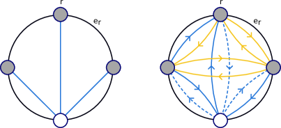
Figure 6: An example of a SRAP instance on the left, where all three undirected links have cost 1. The grey nodes are terminals. The completed instance is shown on the right, where the blue links have cost 1 and the orange links have cost 2 (only the directed links are shown). The dashed blue arcs form a feasible directed solution of cost 3, but there is no $R$-special solution of cost at most 3.

Notice that Theorem 8.1 implies that the maximization step in step 6 of Algorithm 2 can be performed in polynomial time. The following lemma, whose proof is identical to Lemma 9.3 in [18], shows that the algorithm will terminate after polynomially many iterations. Let OPT denote the cost of the optimal augmentation.

Lemma 9.2.

Algorithm 2 runs for at most

$$\ln{\Big{(}\frac{1.5\cdot c(S)}{\text{OPT}}\Big{)}}\cdot\frac{6|R|}{\varepsilon}$$

iterations where $S$ is the initial SRAP solution.

Finally, the solution returned has cost at most $(1.5+\varepsilon)\text{OPT}$.

Lemma 9.3.

At the end of Algorithm 2, we have $c(S)\leq(1.5+\varepsilon)\text{OPT}$.

The proof of the above lemma uses the same potential function analysis which is has been used in [17][18][20], so we do not reproduce it again here. These yield the main result of this section:

Theorem 9.4.

Algorithm 2 is a $(1.5+\varepsilon)$-approximation algorithm for SRAP when $R=V(H)$.

Corollary 9.5.

There is a polynomial time $(1.5+\varepsilon)$-approximation algorithm for $k$-SAG.

Algorithm 2 Local search algorithm for SRAP

Input: A complete instance of SRAP with graph $G=(V,E\dot{\cup}L)$, ring $H=(R,E)$, and $c:L\to\mathbb{R}$. Also a constant $1\geq\varepsilon>0$.
Output: A solution $S\subseteq L$ with $c(S)\leq(1.5+\varepsilon)\text{OPT}$.

1. Compute an arbitrary SRAP solution $S\subseteq L$. Construct witness sets $W_{f}$ for each $f\in S$ so that $\vec{F}:=\bigcup_{f\in S}W_{f}$ is an $R$-special directed solution.

2. Let $\varepsilon^{\prime}:=\frac{\varepsilon/2}{1.5+\varepsilon/2}$ and $\gamma:=2^{\lceil{1/\varepsilon^{\prime}}\rceil}$.

3. For each $A\subseteq R$ where $|A|\leq\gamma$, compute the cheapest full component joining $A$ and denote the cost by $c_{A}$.

4. Create an instance of $\gamma$-restricted Hyper-SRAP on ring $H=(R,E)$ with hyper-links $\mathcal{L}=\{\ell_{A}:A\subseteq R,|A|\leq\gamma\}$. Set the cost of hyper-link $\ell_{A}$ to be $c_{A}$.

5. Let $\alpha:=\lceil 8/\varepsilon\rceil$

6. Iterate the following as long as $\Phi(S)$ decreases in each iteration by at least a factor $(1-\frac{\varepsilon}{12n})$:

   1. Compute the $\alpha$-thin subset of hyper-links $Z\subseteq\mathcal{L}$ maximizing $\bar{c}(\text{drop}_{\vec{F}}(Z))-1.5\cdot c(Z)$, where $\vec{F}:=\bigcup_{f\in S}W_{f}$.

   2. Update the witness sets by replacing each $W_{f}$ with $W_{f}\setminus\text{drop}_{\vec{F}}(Z)$.

   3. Update $S$ by adding all links of full components corresponding to the hyper-links in $Z$.

   4. Shorten directed links in $\vec{F}$ to obtain an $R$-special solution. If $W_{f}=\emptyset$ for some $f\in S$, then remove $f$ from $S$.

7. Return $S$.

References

- [1] Al Borchers and Ding-Zhu Du. Thek-steiner ratio in graphs. SIAM Journal on Computing, 26(3):857–869, 1997.
- [2] Federica Cecchetto, Vera Traub, and Rico Zenklusen. Bridging the gap between tree and connectivity augmentation: unified and stronger approaches. In Proceedings of the 53rd Annual ACM SIGACT Symposium on Theory of Computing, pages 370–383, 2021.
- [3] Joseph Cheriyan, Howard Karloff, Rohit Khandekar, and Jochen Könemann. On the integrality ratio for tree augmentation. Operations Research Letters, 36(4):399–401, 2008.
- [4] Nachshon Cohen and Zeev Nutov. A -approximation algorithm for minimum-cost 2-edge-connectivity augmentation of trees with constant radius. Theoret. Comput. Sci., 489/490:67–74, 2013.
- [5] Efim A Dinitz, Alexander V Karzanov, and Michael V Lomonosov. On the structure of the system of minimum edge cuts in a graph. Issledovaniya po Diskretnoi Optimizatsii, pages 290–306, 1976.
- [6] Yefim Dinitz and Alek Vainshtein. The connectivity carcass of a vertex subset in a graph and its incremental maintenance. In Proceedings of the twenty-sixth annual ACM symposium on Theory of computing, pages 716–725, 1994.
- [7] Stuart E Dreyfus and Robert A Wagner. The steiner problem in graphs. Networks, 1(3):195–207, 1971.
- [8] T. Fleiner and A. Frank. A quick proof for the cactus representation of mincuts. 2009.
- [9] Greg N Frederickson and Joseph Ja’Ja’. Approximation algorithms for several graph augmentation problems. SIAM Journal on Computing, 10(2):270–283, 1981.
- [10] Waldo Gálvez, Fabrizio Grandoni, Afrouz Jabal Ameli, and Krzysztof Sornat. On the cycle augmentation problem: hardness and approximation algorithms. Theory of Computing Systems, 65(6):985–1008, 2021.
- [11] Anupam Gupta and Jochen Könemann. Approximation algorithms for network design: A survey. Surveys in Operations Research and Management Science, 16(1):3–20, 2011.
- [12] Kamal Jain. A factor 2 approximation algorithm for the generalized steiner network problem. Combinatorica, 21(1):39–60, 2001.
- [13] Guy Kortsarz, Robert Krauthgamer, and James R Lee. Hardness of approximation for vertex-connectivity network design problems. SIAM Journal on Computing, 33(3):704–720, 2004.
- [14] Guy Kortsarz and Zeev Nutov. Approximating minimum cost connectivity problems. In Dagstuhl Seminar Proceedings. Schloss Dagstuhl-Leibniz-Zentrum für Informatik, 2010.
- [15] Zeev Nutov. Approximating steiner networks with node-weights. SIAM Journal on Computing, 39(7):3001–3022, 2010.
- [16] Ojas Parekh, R. Ravi, and Michael Zlatin. On small-depth tree augmentations. CoRR, abs/2111.00148, 2021.
- [17] R Ravi, Weizhong Zhang, and Michael Zlatin. Approximation algorithms for steiner tree augmentation problems. In Proceedings of the 2023 Annual ACM-SIAM Symposium on Discrete Algorithms (SODA), pages 2429–2448. SIAM, 2023.
- [18] Vera Traub and Rico Zenklusen. A (1.5+epsilon)-approximation algorithm for weighted connectivity augmentation. arXiv preprint arXiv:2209.07860, 2022.
- [19] Vera Traub and Rico Zenklusen. A better-than-2 approximation for weighted tree augmentation. In 2021 IEEE 62nd Annual Symposium on Foundations of Computer Science (FOCS), pages 1–12, 2022.
- [20] Vera Traub and Rico Zenklusen. Local search for weighted tree augmentation and steiner tree. In Proceedings of the 2022 Annual ACM-SIAM Symposium on Discrete Algorithms (SODA), pages 3253–3272. SIAM, 2022.
- [21] David P Williamson, Michel X Goemans, Milena Mihail, and Vijay V Vazirani. A primal-dual approximation algorithm for generalized steiner network problems. In Proceedings of the twenty-fifth annual ACM symposium on Theory of computing, pages 708–717, 1993.