BREATHE: Second-Order Gradients and Heteroscedastic Emulation based Design Space Exploration

Abstract.

Researchers constantly strive to explore larger and more complex search spaces in various scientific studies and physical experiments. However, such investigations often involve sophisticated simulators or time-consuming experiments that make exploring and observing new design samples challenging. Previous works that target such applications are typically sample-inefficient and restricted to vector search spaces. To address these limitations, this work proposes a constrained multi-objective optimization (MOO) framework, called BREATHE, that searches not only traditional vector-based design spaces but also graph-based design spaces to obtain best-performing graphs. It leverages second-order gradients and actively trains a heteroscedastic surrogate model for sample-efficient optimization. In a single-objective vector optimization application, it leads to 64.1% higher performance than the next-best baseline, random forest regression. In graph-based search, BREATHE outperforms the next-best baseline, i.e., a graphical version of Gaussian-process-based Bayesian optimization, with up to 64.9% higher performance. In a MOO task, it achieves up to 21.9$\times$ higher hypervolume than the state-of-the-art method, multi-objective Bayesian optimization (MOBOpt). BREATHE also outperforms the baseline methods on most standard MOO benchmark applications.

1. Introduction

The number and complexity of applications that require search over a large design space to obtain well-performing solutions are increasing at a significant rate. Various scientific studies aim to search for the best design option in the context of diverse applications, from transistor modeling to astronomical experiments. For instance, modeling the effects of the geometric parameters of a nanowire field-effect transistor on hot-carrier injection (Chen et al., 1985) (to study transistor reliability) requires several measurements on a diverse set of parameter choices (Gupta et al., 2020). Each measurement involves the application of a linear sweep over the drain and gate voltages ($V_{ds}=V_{gs}$) to analyze transistor gate degradation due to hot (energetic) carriers trapped in the gate dielectric. In cosmology, the likelihood of the Lyman-alpha transition (Draine, 2010) provides strong constraints on cosmological parameters and intergalactic medium features, quantities of great interest to astrophysicists. Extracting the likelihood, however, requires simulations to be performed in a high-dimensional parametric space (Rogers et al., 2019). Other domains that require efficient design space exploration include neural architecture search (NAS) (Geifman and El-Yaniv, 2018), cyber-physical systems (Terway et al., 2022), qubit design (Siddiqi, 2021), and many more. However, these studies either involve computationally expensive simulators or time-consuming real-world experimentation, and searching the entire design (or parametric) space via a brute-force approach is typically not possible.

Several black-box optimization methods target efficient search of a design space (Bajaj et al., 2021). These include random search, regression trees, Gaussian-process-based Bayesian optimization (GP-BO), random forest regression, etc. However, gradient descent typically outperforms these traditional gradient-free approaches. For instance, gradient-based optimization outperforms traditional methods in the domain of NAS (Audet and Hare, 2017; Tuli et al., 2023a; Liu et al., 2019). However, leveraging this approach requires a differentiable surrogate of the black-box one wishes to optimize. Moreover, there is often a lack of knowledge and skill in machine learning (ML) among domain experts (device physicists, astronomers, etc.) in order to develop and optimize such surrogate models. Hence, there is a need for a plug-and-play sample-efficient gradient-based optimization pipeline that is applicable to diverse domains with variegated input/output constraints.

To tackle the abovementioned challenges, we propose a novel optimization method, Bayesian optimization using second-order gradients on an actively trained heteroscedastic emulator (BREATHE). It is an easy-to-use approach for efficient search of diverse design spaces where input simulation, experimentation, or annotation is computationally expensive or time-consuming. BREATHE is applicable to both vector and graph optimization. We call the corresponding versions V-BREATHE and G-BREATHE, respectively. G-BREATHE is a novel graph-optimization approach that optimizes both the graph architecture and its components (node and edge weights) to maximize output performance while honoring user-defined constraints. Rigorous experiments demonstrate the benefits of our proposed approach over baseline methods for diverse applications.

The main contributions of the article are as follows.

• We propose V-BREATHE, an efficient vector optimization method, that is widely applicable to diverse domains. It leverages gradient-based optimization using backpropagation to the input (GOBI) (Tuli et al., 2021) implemented on a heteroscedastic surrogate model (Wang et al., 2016). It executes output optimization and supports constraints on the input or output. We propose the concept of legality-forcing on gradients to support constrained optimization and leverage gradients in discrete search spaces. To handle output constraint violations, we use penalization on the output. V-BREATHE requires minimal user expertise in ML.

• We propose G-BREATHE to apply BREATHE to graphical problems. It is a graph optimization framework that searches for the best-performing graph architecture while optimizing the node and edge weights as well. It supports multi-dimensional node and edge weights, thus targeting a much larger set of applications than vector optimization.

• We further enhance V-BREATHE and G-BREATHE to support multi-objective optimization where the desired output is a set of non-dominated solutions that constitute the Pareto front for a given problem. Using multiple random cold restarts, when implementing GOBI, our optimization pipeline can even tackle non-convex Pareto fronts. Our proposed approach achieves a considerably higher hypervolume with fewer queried samples than baseline methods.

The rest of the paper is organized as follows. Section 2 presents background material on vector and graph optimization methods. Section 3 illustrates the BREATHE algorithm in detail. Section 4 describes the experimental setup and the baselines that we compare against. Section 5 explains the results. Section 6 discusses the results in more detail and points out the limitations of the proposed approach. Finally, Section 7 concludes the article.

2. Background and Related Work

In this section, we provide background and related work on optimization using an actively-trained surrogate model.

2.1. Vector Optimization

We refer to the optimization of a multi-dimensional vector (say, $x\in\mathbb{R}^{d}$) as vector optimization. Its application to a black-box function falls under the domain of black-box optimization. Mathematically, one can represent this problem as follows.

(1) $$\min F(x)$$

s.t. $$x^{L}_{i}\leq x_{i}\leq x^{U}_{i}\ i=1,\ldots,d$$

Here, $F$ is the black-box function we need to optimize; $x_{i}$ is the $i$-th variable in the design space; $x^{L}_{i}$ and $x^{U}_{i}$ are its lower and upper bounds. We may not have a closed-form expression for $F$ (a black-box); thus, finding a solution $x^{*}$ may not be easy.

Many works target vector optimization. Random search uniformly samples inputs within the given bounds. Gradient-boosted regression trees (GBRTs) model the output using a set of decision trees (Ke et al., 2017). GP-BO (Snoek et al., 2012) approximates performance through Gaussian process regression and optimizes an acquisition function through the L-BFGS method (Liu and Nocedal, 1989). Other optimization methods leveraging a GP-based surrogate suffer from the bottlenecking $\mathbf{argmax}$ operation over the entire design space (De Ath et al., 2021). Random forests fit various randomized decision trees over sub-samples of the dataset. BOSHNAS (Tuli et al., 2023a) searches for the best neural network (NN) architecture for an ML task. It outperforms other optimization techniques in the application of NAS to convolutional NNs (Tuli et al., 2023b) and transformers (Tuli et al., 2023a). These approaches rely on active learning (Ren et al., 2021), in which the surrogate model, which can be a regression tree or an NN, interactively queries the simulator (or the experimental setup) to label new data. We use the new data to update the model at each iteration. This updated model forms new queries that lead to higher predicted performance. We iterate through this process until it meets a convergence criterion. Finally, this yields the input with the best output performance.

The abovementioned approaches do not consider optimization under constraints. Optimizing the objective function while adhering to user-defined constraints falls under the domain of constrained optimization. Mathematically,

(2) $$\min F(x)$$

s.t. $$x^{L}_{i}\leq x_{i}\leq x^{U}_{i}\ i=1,\ldots,d$$

$$C^{I}_{j}(x)\leq 0\ j=1,\ldots,J^{\prime}$$

$$C^{E}_{k}(x)=0\ k=1,\ldots,K^{\prime}$$

for $J^{\prime}$ inequality constraints and $K^{\prime}$ equality constraints. One can convert each equality constraint to two inequality constraints. Thus, we can simplify the above problem as follows:

(3) $$\min F(x)$$

s.t. $$x^{L}_{i}\leq x_{i}\leq x^{U}_{i}\ i=1,\ldots,d$$

$$C_{j}(x)\leq 0\ j=1,\ldots,J$$

where $J=J^{\prime}+2K^{\prime}$.

This problem belongs to the class of constrained single-objective optimization (SOO) problems. One could also search the input space to optimize multiple objectives simultaneously while honoring the input constraints. We refer to this class of problems as constrained multi-objective optimization (MOO) problems (Deb, 2011). Mathematically,

(4) $$\min F_{m}(x)\ m=1,\ldots,M$$

s.t. $$x^{L}_{i}\leq x_{i}\leq x^{U}_{i}\ i=1,\ldots,d$$

$$C_{j}(x)\leq 0\ j=1,\ldots,J$$

for $M$ objective functions.

Previous works propose various methods to solve MOO problems. Non-dominated sorting genetic algorithm-2 (NSGA-2) (Deb et al., 2002) is a seminal evolutionary algorithm (EA)-based optimization method that evolves a set of candidates across generations into better-performing solutions. Multi-objective evolutionary algorithm based on decomposition (MOEA/D) (Zhang and Li, 2007) is another popular EA-based method that decomposes a MOO problem into multiple SOO problems and optimizes them simultaneously. Many state-of-the-art search techniques are based on evolutionary methods (Chugh et al., 2019; Rahi et al., 2022). Since the proposed approach is a surrogate-based method, we only compare it against the representative EA-based methods mentioned above. Multi-objective regionalized Bayesian optimization (MORBO) (Daulton et al., 2022) is a MOO framework based on Bayesian optimization (BO). It performs BO in multiple local regions of the design space to identify the global optimum. MOBOpt (Galuzio et al., 2020) is yet another surrogate-based Bayesian optimization framework for MOO problems. The proposed V-BREATHE algorithm solves both SOO and MOO problems.

2.2. Graph Optimization

In the above scenario, input $x\in\mathbb{R}^{d}$ is a vector. However, in many applications, $x$ may be a graph, i.e., $x\in\mathcal{G}$, where $\mathcal{G}$ is the space of legal graphs (see Section 3.1.4). In this scenario, graph optimization refers to searching for an input graph that optimizes (single or) multiple output objectives under given constraints. Mathematically,

(5) $$\min F_{m}(x)\ m=1,\ldots,M$$

s.t. $$x\in\mathcal{G}$$

$$C_{j}(x)\leq 0\ j=1,\ldots,J$$

where we define $\mathcal{G}$ based on a set of legal node connections (edges) along with node and edge weight bounds.

Traditional works on graph optimization target specific problems, such as max-flow/min-cut (Leighton and Rao, 1999), graph partitioning (Buluç et al., 2016), graph coloring (Jensen and Toft, 2011), routing (Applegate et al., 2011), etc. However, these optimization problems aim to either find a subset of a given graph or annotate a given graph. In this work, we target an orthogonal problem: find the best-performing graph for the given objective function(s). This involves searching for the set of nodes (or vertices) and edges along with their weights. Existing works solve this problem with limited scope, i.e., they may not consider all graph constraints (Terway et al., 2022) (when converting the problem into vector optimization) or are only applicable to NN models (Geifman and El-Yaniv, 2018). Moreover, graph optimization involves searching for not only the node/edge values (which could be represented as multi-dimensional vectors) but also the connections. Directly flattening a graph and implementing vector optimization methods does not perform well, as we show in this work, as such methods would not be able to look for new connections that modify the graph architecture. This calls for novel search techniques that directly implement optimization on graphical input. The proposed G-BREATHE algorithm solves both SOO and MOO graph problems.

3. Methodology

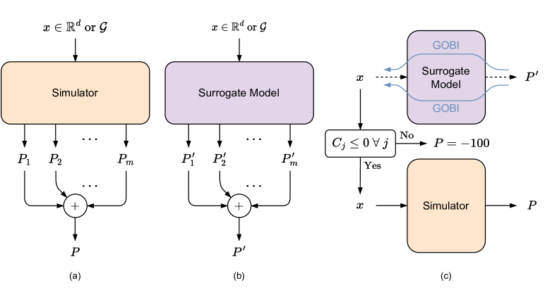
Figure 1. Overview of the BREATHE framework. (a) The simulator takes an input $x$, which can be a vector (in $\mathbb{R}^{d}$) or a graph (in $\mathcal{G}$). It outputs the performance value corresponding to each objective ($P_{i}$). $P$ is a convex combination of individual performance measures for SOO. (b) The surrogate model is a lightweight (i.e., computationally inexpensive relative to the simulator) and differentiable emulator that mimics the simulator; its predicted performance is $P^{\prime}$. (c) GOBI is applied to the surrogate model to obtain $x$ with a higher predicted performance $P^{\prime}$. The dataset is updated with the simulated value $P$ to enable retraining of the surrogate model.

In this section, we discuss the BREATHE framework that leverages GOBI on a heteroscedastic surrogate model. Fig. 1 summarizes the BREATHE framework.

3.1. V-BREATHE

V-BREATHE is a widely-applicable vector-input-based optimizer that runs second-order gradients on a lightweight NN-based surrogate model to predict not only the output objective value but also its epistemic and aleatoric uncertainties. It leverages an active-learning framework to optimize the upper confidence bound (UCB) estimate of the output objective. In this context, we freeze the model weights and backpropagate the gradients to update the input (not the model weights) to optimize the output objective. We then query the simulator to obtain the output of the new queried sample and retrain the surrogate model. This iterative search process continues until convergence. We describe the V-BREATHE optimizer in detail next.

3.1.1. Uncertainty Types

Prediction uncertainty may arise from not only the approximations made in the surrogate modeling process or limited data and knowledge of the design space but also the natural stochasticity in observations. The former is termed epistemic uncertainty and the latter aleatoric uncertainty. The epistemic uncertainty, also called reducible uncertainty, arises from a lack of knowledge or information, and the aleatoric uncertainty, also called irreducible uncertainty, refers to the inherent variation in the system to be modeled.

In addition, uncertainty in output observations may also be data-dependent (known as heteroscedastic uncertainty). Accounting for such uncertainties in the optimization objective requires a surrogate that also models them.

3.1.2. Surrogate Model

Following the surrogate modeling approach used in BOSHNAS (Tuli et al., 2023a), a state-of-the-art NAS framework, we model the output objective and aleatoric uncertainty using a natural parameter network (NPN) (Wang et al., 2016) $f(x;\theta)$. We model the epistemic uncertainty using a teacher network $g(x;\theta^{\prime})$ and its student network $h(x;\theta^{\prime\prime})$. Here, $\theta$, $\theta^{\prime}$, and $\theta^{\prime\prime}$ refer to the trainable parameters of the respective models. We leverage GOBI on $h$ to avoid numerical gradients due to their poor performance (Tuli et al., 2023a). We have $(\mu,\sigma)\leftarrow f(x;\theta)$, where $\mu$ is the predicted output objective (i.e., a surrogate of $F$) and $\sigma$ is the aleatoric uncertainty. Moreover, $h$ predicts a surrogate ($\hat{\xi}$) of the epistemic uncertainty ($\xi$). The teacher network $g$ models the epistemic uncertainty via Monte Carlo dropout (Tuli et al., 2023a).

We model the output objective in the $[0,1]$ interval for easier convergence. We implement this in the surrogate model by feeding the output to a sigmoid activation. To implement this, we normalize the output objective $F$ with respect to its maximum permissible value and maximize the performance measure:

(6) $$P=1-\frac{F}{F^{MAX}},\quad\ F^{MAX}=M_{O}\max_{x,\forall(x,P)\in\Delta}F$$

where $\Delta$ is the set of currently observed samples in the design space and $M_{O}\geq 1$ is a multiplicative overhead factor. If we observe a larger value during the search process, we re-annotate the observed data with the updated value of $F^{MAX}$ and retrain the lightweight surrogate model.

3.1.3. Active Learning and Optimization

To use GOBI and obtain queries that perform well, we initialize the surrogate model by training it on a randomly sampled set of points in the design space. We call this set the seed dataset. To effectively explore globally optimal design points, the seed dataset should be as representative of the design space as possible. For this, we use low-discrepancy sequence sampling strategies (Niederreiter, 1992). Specifically, V-BREATHE uses Latin hypercube sampling to obtain divergent points in its sampled set (parallel works show that this indeed performs better than other low-discrepancy sampling methods in maximizing the diversity of the sampled points (Tuli and Jha, 2023)). We evaluate these $N_{\Delta_{0}}$ initial samples using the (albeit expensive) simulator and train the surrogate model on this seed dataset $\Delta_{0}$. Then, we run second-order optimization on

(7) $$\text{UCB}=\mu+k_{1}\cdot\sigma+k_{2}\cdot\hat{\xi}$$

where $k_{1}$ and $k_{2}$ are hyperparameters. We employ the UCB estimate instead of other acquisition functions as it results in the fastest convergence as per previous works that leverage gradient-based optimization (Tuli et al., 2023a, b). Nevertheless, we leave the application of other acquisition functions to future work.

3.1.4. Incorporating Constraints

Since one cannot directly add symbolic constraints to an NN, we train the surrogate model with a sample with very low performance value that does not satisfy the output constraints (also called penalization). For instance, if an output $F_{m}$ does not meet a constraint (say, $C_{j^{\prime}}>0$), we set the corresponding performance to $P=-100$, which should otherwise be in the $[0,1]$ interval. This forces the surrogate model to learn the distribution of input samples that do not satisfy the desired output constraints.

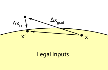
Figure 2. Schematic illustration of legality-forcing. GOBI results in the gradient step $\Delta x_{\text{grad}}$ that is outside the set of legal inputs (which may be a subset of the design space). $\Delta x_{\text{LF}}$ implements a step forcing the resultant input to be legal.

While running GOBI, if the updated input at an epoch does not satisfy the constraints (i.e., is an illegal input), we set it to the nearest legal input (based on Euclidean distance) that satisfies the constraints. One can consider this as adding an additional force while running gradient descent in the input space that iteratively makes the updated input legal. We call this approach legality-forcing. Fig. 2 explains this using a working schematic.

3.1.5. Simultaneous Optimization of Multiple Objectives

To support MOO with V-BREATHE, we need to run GOBI to obtain new input queries that optimize all $F_{m}$ in Eq. (4). To tackle this problem, one could try to optimize a sum of all objectives. However, each point on the Pareto front weights each objective differently. Hence, we optimize multiple convex combinations of $F_{m}$’s. More concretely,

(8) $$P=\sum_{m}\alpha_{m}P_{m},\quad m=1,\ldots,M$$

where $P_{m}$ is a function of $F_{m}$ as per Eq. (6) and $\alpha_{m}$’s, where $\sum_{m}\alpha_{m}=1$, are hyperparameters that determine the weight assigned to each objective. Thus, different samples of these weights would result in different non-dominated solutions, i.e., points on the Pareto front. In this context, V-BREATHE maximizes the performance measure $P$ for every set of weight samples using GOBI.

3.2. G-BREATHE

G-BREATHE implements the V-BREATHE algorithm on graphical input. Instead of using a fully-connected NN, which assumes a vector input, we use a graph transformer (Shi et al., 2021) network as our surrogate model. We use a graph transformer as it is a state-of-the-art model for graphical input. We characterize the input graph by its nodes, edges, and multi-dimensional weight values.

While running GOBI, we backpropagate the gradients to the node and edge weights. If all the edge weights fall below a threshold ($\epsilon_{E}=10^{-5}$ for non-binary edge weights and $\epsilon_{E}=0.5$ for binary edge weights), we remove that edge. To explore diverse graphs with varied node/edge combinations and weights, we sample randomly generated graphs at each iteration of the search process and run GOBI on the trained surrogate to look for better versions of those graphs (i.e., with the same connections but different node/edge weights that maximize performance). The rest of the setup is identical to that of V-BREATHE. From now on, we will use the term BREATHE to refer to either V-BREATHE or G-BREATHE based on the input type unless otherwise specified.

Result: best $x$

1 Initialize: convergence criterion, uncertainty sampling prob. ($\alpha$), diversity sampling prob. ($\beta$), surrogate model ($f$, $g$, and $h$), initial dataset $\Delta_{0}$, design space $\mathcal{D}$, $i=0$;

2while convergence criterion not met do

3       if prob. $\sim U(0,1)<1-\alpha-\beta$ then

4             fit($f$, $g$, $h$; $\Delta_{i}$);

             $x$ $\leftarrow$ GOBI($f$, $h$);

              /* Optimization step */

5             $P\leftarrow\textnormal{{{simulate}}}$($x$);

6       else

7             if $1-\alpha-\beta\leq$ prob. $<1-\beta$ then

                   $x$ $\leftarrow$ argmax($k_{1}\cdot\sigma+k_{2}\cdot\hat{\xi}$);

                    /* Uncertainty sampling */

8                  

9             else

10                   $x\leftarrow\textnormal{{{random}}}$($\mathcal{D}$);

                  

                    /* Diversity sampling */

11                  

12             $C\leftarrow$ True;

13             for $j=1$ to $J$ do

14                   if $C_{j}(x)>0$ then

                         $C\leftarrow$ False;

                          /* Output constraint not satisfied */

15                         break;

16            if $C$ is True then

17                   $P\leftarrow\textnormal{{{simulate}}}$($x$);

18             else

19                   $P\leftarrow-100$;

20            

21       $i\leftarrow i+1$;

22      $\Delta_{i}\leftarrow(x,P)\cup\Delta_{i-1}$;

Algorithm 1 BREATHE

Algorithm 1 summarizes the BREATHE algorithm (for both SOO and MOO settings). Starting from an initial seed dataset $\Delta_{0}$, we run the following steps until convergence. To trade off between exploration and exploitation, we consider two probabilities: uncertainty-based exploration ($\alpha$) and diversity-based exploration ($\beta$). With probability $1-\alpha-\beta$, we run second-order GOBI using the surrogate model to maximize the UCB in Eq. (7). To achieve this, we first train the surrogate model (a combination of $f$, $g$, and $h$) on the current dataset (line 1). For SOO, we initialize only one surrogate model, however, for MOO, we initialize separate surrogate models for each set of randomly initialized $\alpha_{m}$’s. We then generate a new query point by freezing the weights of $f$ and $h$ and run GOBI along with legality-forcing to obtain an $x$ (adhering to constraints) with better-predicted performance (line 1). We then simulate the obtained query to obtain the performance measure $P$ (line 1). For SOO, this corresponds to a single $\alpha_{1}=1$, but for MOO, this corresponds to a random selection of $\alpha_{m}$’s, and we obtain $P$ as per Eq. (8). With $\alpha$ probability, we sample the search space using the combination of aleatoric and epistemic uncertainties, $k_{1}\cdot\sigma+k_{2}\cdot\hat{\xi}$, to find a point where the performance estimate is the most uncertain (line 1). We also choose a random point with probability $\beta$ (line 1) to avoid getting stuck in a localized search subset. The exploration steps also aid in reducing the inaccuracies in surrogate modeling for unexplored regions of the design space. Finally, we run the simulation only if the obtained input adheres to user-defined constraints ($C_{j}$’s in Eqs. (3), (4), and (5)), and penalize the output performance by setting $P=-100$ otherwise (line 1).

4. Experimental Setup

In this section, we present the setup behind various experiments, including the applications for vector and graph optimization, baselines for comparison, and details of the surrogate models.

4.1. Evaluation Applications

The applications with which we test our optimizers include two in the domain of vector optimization: operational amplifier (op-amp) and waste-water treatment plant (WWTP), and two in the domain of graph optimization: smart home and network. We also test the V-BREATHE algorithm against previously-proposed MOO baselines on standard benchmarks. Finally, we use the problem of synchronous optimal pulse-width modulation (SO-PWM) of three-level inverters for scalability analysis. We describe each application in detail next.

4.1.1. Op-amp

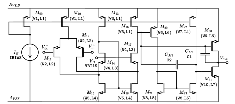
Figure 3. Circuit diagram of the three-stage op-amp. Variables that constitute the input design space are presented in typewriter font.

This application involves the optimization of a three-stage op-amp featuring a positive-feedback frequency compensation technique (Eschauzier and Huijsing, 1995). It has 24 input variables (supply/bias voltages and currents, load resistance, load capacitance, transistor widths and lengths, etc.), three constraints (lower/upper limits on DC gain, phase margin, and unity gain frequency), and one optimization objective (minimization of power consumption). We implement the simulations using the Cadence Spectre circuit simulator (spe, 2023).

Fig. 3 shows a circuit diagram of the op-amp along with the variables involved in the optimization process. $M_{00}$ is the bias metal-oxide semiconductor field-effect transistor (MOSFET). $M_{10}$, $M_{11}$, and $M_{12}$ are part of the differential pair. $M_{13}$-$M_{18}$ are part of the folded cascode. MOSFETs $M_{20}$-$M_{23}$ constitute the second stage, while $M_{30}$ and $M_{31}$ constitute the third stage of the op-amp. We use two compensation capacitors: $C_{M1}$ and $C_{M2}$. The input optimization space comprises 24 variables. These include 10 MOSFET widths (W1-W10), seven MOSFET lengths (L1-L7), capacitor values (C1 and C2), bias voltage (VBIAS), bias current (IBIAS), load resistance (RLOAD), load capacitance (CLOAD), and supply voltage (VSUPPLY).

We constrain the DC gain to be greater than 68, the phase margin to be between 31.8°and 130.0°, and the unity gain frequency to be greater than 1.15 MHz (asc, 2023).

4.1.2. WWTP

Waste-water treatment removes contaminants and converts waste water into an effluent that one can return to the water cycle. Specifically, we consider the four-stage Bardenpho process (Esfahani et al., 2018). Optimizing the WWTP involves 14 input variables (flow split percentages along with reactor volumes, temperatures, and dissolved oxygen levels) and four output objectives [fractions of chemical oxygen demand (COD), namely $S_{I}$: inert soluble, $S_{S}$: readily biodegradable, $X_{I}$: inert particulate, and $X_{S}$: slowly biodegradable compounds]. For SOO, we optimize the net COD as a sum, i.e., $S_{I}+S_{S}+X_{I}+X_{S}$. However, for MOO, we optimize all objectives simultaneously to obtain commonly-studied Pareto fronts: $S_{I}$ vs. $S_{S}$ and $X_{I}$ vs. $X_{S}$. We use a publicly available simulation software for evaluating different WWTPs.

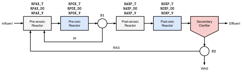
Figure 4. Simplified schematic of the four-stage Bardenpho process. Variables that constitute the input design space are presented in typewriter font.

Fig. 4 shows a simplified schematic of the four-stage Bardenpho process. It consists of four reactors and a secondary clarifier. There are three design parameters for each reactor, namely, the maintained temperature (in °C), the dissolved oxygen (DO, in mg/L), and the reactor volume (in m³). The first split ($\texttt{S1}\in[1,8]$) determines the amount of sludge for internal re-circulation (IR). The second split ($\texttt{S2}\in[0,1]$) determines the ratio of return-activated sludge (RAS) and waste-activated sludge (WAS). This results in 14 input variables for optimization. We limit the temperatures in the range 5-15 °C, volumes in 100-15000 m³, and DO in 0-5 mg/L. These ranges are typically used in many plants.

4.1.3. Smart Home

A smart home consists of multiple Internet-of-Things (IoT) devices. These include smart doorbells, smart locks, entry/exit sensors, smart door cameras, home assistants, smart thermostats, etc. We support different network types, namely WiFi, Zigbee (zig, 2023), and Z-Wave (zwa, 2023). Further, we need to connect different room types (hall, master bedroom, bedrooms, entry hall, living room, kitchen/dining area, and outside porch). Each room can also have multiple IoT devices. The task is to design a smart home, with constraints on the total number of windows and the total area, that minimizes the number of cyber-physical attacks (one optimization objective). For instance, an attacker could use a light command to maliciously manipulate devices in rooms with windows (given that the devices use Zigbee or Z-Wave and have a clear line of sight through the windows in the room). We used a Python-based simulator for testing our proposed optimizer.

We now describe the graph formulation of a smart home in G-BREATHE. There can be a total of 9 nodes, one for each room type, except bedrooms, which can be three in number. We represent each node (or room) by a 12-dimensional weight vector consisting of categorical and continuous features. The weight vector includes the room type, room area, number of windows, number of each IoT device (we support a total of eight devices), and the type of network used. We restrict all the devices in a smart home to only one network type (although the WiFi router always connects to the gateway via a WiFi connection). An edge weight is a Boolean value, i.e., whether the two nodes are connected or not. There are three constraints: the total number of windows should be more than or equal to three, the total area of the smart home should be greater than 300 m² and less than 600 m², and the network connection for all IoT devices should be the same. Table 1 summarizes the design parameters for the smart home application.

Table 1. Design parameters associated with the smart home application. The table shows the number of rooms allowed in the graph along with their area limits. It also shows the total number of IoT devices allowed in a smart home for each device type (S.: Smart).

Room Types
Design Space Parameter	Hall	Master Bedroom	Bedroom		Entry Hall	Living Room	Kitchen/Dining	Porch
Number	1	1	1-3		1	1	1	1
Area (m2)	10-50	24-100	10-50		10-40	50-120	50-100	80-120
IoT Devices
Design Space Parameter	WiFi Modem	S. Doorbell	Gateway	S. Lock	Entry Sensor	S. Door Camera	Home Assistant	S. Thermostat
Number	1	1	1	1	1-3	1	1-8	1-3

4.1.4. Network

Higher bandwidth and lower latency connections available in modern networks (Gill et al., 2019) have enabled the network edge to execute substantially more computations. However, the simulation of urban mobility (SUMO) domain (Krajzewicz et al., 2012) demands computationally-expensive simulations that must run frequently to ensure stable connections. In this application, we optimize the number of switches and their connections with data sources and mobile/edge data sinks (thus, forming a network graph) to maximize bandwidth and minimize network operation costs.

Each graph may have up to 25 nodes (five data sources, five data sinks, and up to 15 switches). The node weight represents the type of node: data source/sink or switch. Edges between nodes represent the bandwidth of the corresponding network connection (restricted from 128 MB/s to 1024 MB/s). As explained above, the two optimization objectives are network bandwidth and operation cost.

We set the cost of a data source (typically a cloud server) to $5000 while that of sink to $1000 (an edge device). The cost of a switch is $1000. Adding a connection to the switch incurs an additional base cost of $200, which increases with bandwidth [at the rate of 0.05 $/(MB/s)]. These costs are typical of common devices employed in networking applications.

4.1.5. SO-PWM of Three-level Inverters

Multi-level inverters reduce the total harmonic distortion (THD) in their alternating current (AC) output. SO-PWM control permits setting the maximum switching frequency to a low value without compromising on the THD (Rathore et al., 2010) of the AC output. This application has 25 inputs, 24 constraints, and two optimization objectives. We perform scalability tests in Section 5.5 where we study the effect on best-achieved performance and the number of evaluation queries as we increase the number of tunable inputs or constraints. We implement an adapted version of the MATLAB-based simulator, available from a benchmarking suite (Kumar et al., 2021), for scalability analysis.

We represent the SO-PWM problem (Rathore et al., 2010) in the form of Eq. (4) as follows:

(9) $$\min F_{1}(x)=\frac{\sqrt{\sum_{k}{k^{-4}\sum_{i=1}^{N}S(i)\cos^{2}{(kx_{i})}}}}{\sqrt{\sum_{k}{k^{-4}}}}$$

$$\min F_{2}(x)=\left(0.32-\sum_{i=1}^{N}{S(i)\cos{(x_{i})}}\right)^{2}$$

s.t. $$0<x_{i}<\frac{\pi}{2},\qquad\qquad\quad\ \ i=1,\ldots,N\$$

$$x_{j+1}-x_{j}-10^{-5}>0,\quad\,j=1,\ldots,N-1$$

where, $k=5,7,11,13,\ldots,97$, $N=25$, and $S(i)=(-1)^{i+1}$.

4.1.6. Benchmark Applications

We compare V-BREATHE against baseline methods on standard benchmarks. These include the ZDT problem suite (Zitzler et al., 2000), the Binh and Korn (BNH) benchmark (Binh and Korn, 1997), the Osyczka and Kundu (OSY) benchmark (Osyczka and Kundu, 1995), and the Tanaka (TNK) benchmark (Tanaka et al., 1995). Although these benchmarks are implemented with mathematical formulas that are easy to evaluate, to test the efficacy of various methods in low-data regimes (in the context of a computationally expensive simulator), we start with a low number of randomly sampled points (i.e., 64 in our experiments) in the seed dataset $\Delta_{0}$.

Table 2 summarizes the dimensions involved in each optimization application.

Table 2. Dimensionality of inputs, constraints, and outputs for targeted applications.

Vector Optimization
Application	Inputs			Constraints	Outputs
Op-amp	24			3	1
WWTP	14			0	4
SO-PWM	25			24	2
ZDT1	30			0	2
ZDT2	30			0	2
ZDT3	30			0	2
ZDT4	10			0	2
ZDT5	80			0	2
ZDT6	10			0	2
BNH	2			2	2
OSY	6			6	2
TNK	2			2	2
Graph Optimization
Application	Nodes	Node dim.	Edge dim.	Constraints	Outputs
Smart Home	9	12	1	3	1
Network	25	1	1	0	2

4.2. Surrogate Models

We now present details of the architectural decisions for the surrogate models along with the hyperparameters used in the BREATHE algorithm. For vector optimization, in all three surrogate models $f$, $g$, and $h$, we pass the input through two fully-connected hidden layers with 64 and 32 neurons, respectively. For graph optimization, we pass the input through a graph transformer layer (Shi et al., 2021) with four attention heads, each with a hidden dimension of 16. We then pass the output of the transformer layer to a set of fully-connected layers as above. We show other hyperparameter choices for Algorithm 1, which we obtained through grid search, in Table 3.

Training the surrogate model on the initial dataset, $\Delta_{0}$, for five epochs takes about 300-400 ms on an NVIDIA A100 GPU with a batch size of 64. This is negligible compared to the time taken by the simulator on a single query, e.g., hundreds of seconds (or more) for some applications.

The execution time of the proposed algorithm does not increase with the number of inputs. As the number of inputs increases, the input neurons in the surrogate model increase. However, since the neural network computation is performed in parallel, the execution time remains constant.

Table 3. Selected hyperparameters for the BREATHE algorithm.

Hyperparmeters	Value
$M_{O}$	1.2
$N_{\Delta_{0}}$	64
$k_{1}$, $k_{2}$	0.5, 0.5
$\alpha$, $\beta$	0.1, 0.1

4.3. Baselines

For SOO with vector input, we compare BREATHE against random sampling (Random), random forest regression (Forest), GBRT, and GP-BO. We implement these baselines using the scikit-learn library (Pedregosa et al., 2011) with default parameters. This implies that for random forest regression, we use 100 trees, the Gini index to measure the quality of splits, and the minimum number of samples per split set to two. The GBRT optimizer uses the squared-error loss with a learning rate of 0.1, 100 boosting stages, and the minimum number of samples per split set to two. For MOO, we compare the MOO version of the proposed algorithm with state-of-the-art and popular baselines: NSGA-2, MOEA/D, and MOBOpt. We use the implementation from PyMOO (Blank and Deb, 2020) to run NSGA-2 and MOEA/D in Python. We use the default hyperparameters (in the PyMOO library) for these methods. For MOBOpt, we use the source code with default parameters.

For graph optimization, we compare G-BREATHE against graphical adaptations of the above baselines. To implement this, we randomly generate graphs and only optimize the node/edge weights of the graph by flattening it into a vector and feeding the vector into the vector optimization baseline. We let the baseline search the node/edge weight space for 32 iterations before generating new graphs. This enables these baselines to search in both spaces: graph architecture and node/edge weight values.

5. Results

In this section, we present experimental results and comparisons of the proposed BREATHE optimizer with relevant baselines.

5.1. Single-objective Vector Optimization using BREATHE

For SOO with BREATHE and baselines approaches, we maximize the performance measure $P$ defined in Eq. (8) even if the application has multiple objectives. Unlike MOO, here we choose a fixed combination of $\alpha_{m}$. Only one output objective is associated with op-amp optimization, while WWTP comprises four objectives ($S_{I}$, $S_{S}$, $X_{I}$, and $X_{S}$) that we maximize. We use V-BREATHE for vector input. For SOO, we set $\alpha_{m}=0.25,\ \forall m\in[1,2,3,4]$, for this application, maximizing a simple sum of the COD fractions.

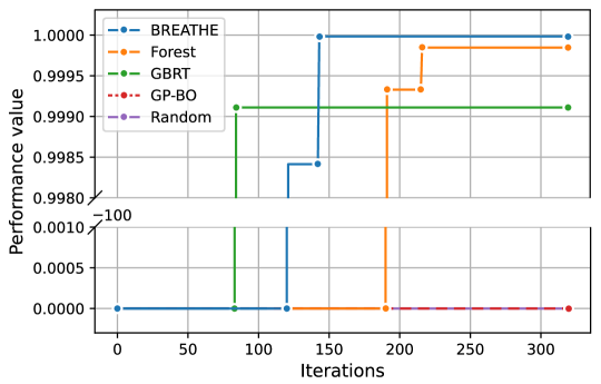
Figure 5. Performance convergence of BREATHE and various baselines on the op-amp application.

Figs. 5 and 6 show the convergence of output performance $P$ for the op-amp and WWTP objectives, respectively. BREATHE achieves the highest performance among all methods. For the op-amp application, none of the methods can initially find input parameters that satisfy all constraints (resulting in the convergence plot to start at $P=-100$). BREATHE, Forest, and GBRT find legal inputs and optimize the output performance using these legal data points. However, GP-BO and random search are not able to find legal inputs that result in $P>-100$, i.e., $P\in[0,1]$. When there are no constraints, GP-BO achieves the second-highest performance in the WWTP application.

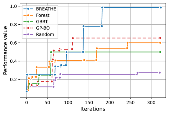
Figure 6. Performance convergence of BREATHE and various baselines on the WWTP application.

Table 4. Selected design parameters of the best-performing points achieved by BREATHE on the op-amp and WWTP applications.

Op-amp
VSUPPLY		VBIAS		IBIAS	CLOAD	RLOAD	C1	C2	L1	L2	L3	L4	L5
2.4 V		2.5 V		7.0 $\mu$A	0.12 nF	10.0 k$\Omega$	2.0 pF	14.0 pF	4.6 $\mu$m	6.3 $\mu$m	2.8 $\mu$m	1.8 $\mu$m	3.8 $\mu$m
L6		L7		W1	W2	W3	W4	W5	W6	W7	W8	W9	W10
2.4 $\mu$m		5.2 $\mu$m		4.4 $\mu$m	18.4 $\mu$m	26.3 $\mu$m	10.4 $\mu$m	34.3 $\mu$m	48.4 $\mu$m	32.4 $\mu$m	22.3 $\mu$m	32.3 $\mu$m	44.4 $\mu$m
WWTP
S1	S2	RPAX_T	RPAX_DO	RPAX_V	RPOX_T	RPOX_DO	RPOX_V	RAXP_T	RAXP_DO	RAXP_V	ROXP_T	ROXP_DO	ROXP_V
1.5	0.9	10.3 C	0.0 mg/L	3067.0 m3	6.2 °C	5.0 mg/L	102.1 m3	5.2 °C	1.5 mg/L	100.0 m3	13.1 °C	3.6 mg/L	100.0 m3

Table 4 summarizes the design parameter values for the op-amp and WWTP applications selected by BREATHE. It chooses the input parameters for resistor and capacitor values along with transistor lengths and widths that maximize the output performance. The DC gain of the op-amp is 90.8, its unity gain frequency is 1.58 MHz, and its phase margin is 95.8°, while incurring 780.2 mW of power. For WWTP, BREATHE chooses a large pre-anoxic reactor (with volume = 3067.0 m³) but much smaller subsequent reactors. Table 4 shows other design decisions as well. This design leads to the maximum net COD.

5.2. Multi-objective Optimization using BREATHE

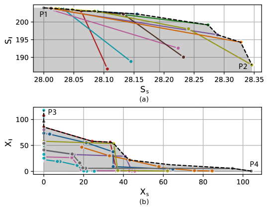
Figure 7. Pareto fronts of (a) $S_{I}$ vs. $S_{S}$ and (b) $X_{I}$ vs. $X_{S}$ using the BREATHE optimizer on the WWTP task. All objectives are plotted in mg/L units.

We now show the MOO performance of BREATHE on the WWTP application with four output objectives. Capturing non-dominated solutions on different parts of the Pareto front would require contrasting weights for each objective. Thus, we take random samples of the objective weights $\alpha_{m}$. Fig. 7 shows the Pareto front while trading off $S_{I}$ for $S_{S}$ and $X_{I}$ for $X_{S}$. These trade-offs are typically studied by domain experts. Different colors correspond to distinct sets of $\alpha_{m}$’s among 16 random samples. We observe that different colors (and thus, weights for the objectives) indeed contribute to unique non-dominated solutions on the Pareto front (shown by dashed line).

Table 5. Selected design parameter values of the four extreme points of the Pareto fronts in Fig. 7 for the WWTP application.

Point Name	WWTP
	S1	S2	RPAX_T	RPAX_DO	RPAX_V	RPOX_T	RPOX_DO	RPOX_V	RAXP_T	RAXP_DO	RAXP_V	ROXP_T	ROXP_DO	ROXP_V
P1	8.0	1.0	15.0 °C	5.0 mg/L	1458.9 m3	15.0 °C	0.0 mg/L	8683.8 m3	15.0 °C	5.0mg/L	2450.3 m3	15.0 °C	0.0 mg/L	2488.9 m3
P2	8.0	1.0	5.0 °C	5.0 mg/L	11299.7 m3	15.0 °C	0.0 mg/L	6899.8 m3	15.0 °C	0.0 mg/L	13400.1 m3	15.0 °C	0.0 mg/L	14900.0 m3
P3	1.0	1.0	15.0 °C	0.0 mg/L	100.0 m3	5.0 °C	0.0 mg/L	1518.9 m3	5.0 °C	0.0 mg/L	152.9 m3	5.0 °C	0.0 mg/L	2779.3 m3
P4	8.0	1.0	5.0 °C	3.7 mg/L	479.9 m3	8.8 °C	5.0 mg/L	3504.1 m3	14.1 °C	5.0 mg/L	311.1 m3	15.0 °C	5.0 mg/L	991.5 m3

Table 6. Output objective values (in mg/L units) for the four extreme points of the Pareto fronts in Fig. 7 for the WWTP application.

Point Name	Output Objectives
	$S_{I}$	$S_{S}$	$X_{I}$	$X_{S}$
P1	204.01	28.00	36.34	0.01
P2	193.93	28.45	13.37	0.27
P3	204.00	27.94	117.64	0.01
P4	1.60	19.52	0.58	104.17

Table 5 summarizes the design choices of the four plants that correspond to the four extrema of the two Pareto fronts (P1-P4) in Fig. 7. P1 corresponds to the plant with the highest achieved $S_{I}$ in the effluent, while P4 corresponds to the plant with the highest achieved $X_{S}$ in the effluent. Table 6 shows the output objective values for the four design points. When we maximize one objective, other objective values are much lower. This implies that there is a trade-off when maximizing all objectives that BREATHE considers by presenting a Pareto front.

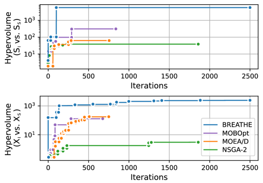
Figure 8. Convergence of hypervolume (in mg²/L² units) of (a) $S_{I}$ vs. $S_{S}$ and (b) $X_{I}$ vs. $X_{S}$ Pareto fronts with the number of iterations when running BREATHE and other MOO baselines on the WWTP task.

We train independent surrogate models for each selection of weights and run the BREATHE optimization pipeline in parallel. We observe that parallel runs outperform sequential operations of the BREATHE algorithm (where we iteratively update the surrogate model on each new dataset with the new set of objective weights). We hypothesize that the independent parallel runs result in a higher variance in the internal representations of the meta-model as it covers a larger fraction of the design space.

Hypervolume is a measure of the solution quality in MOO problems. We derive it by measuring the size of the dominated portion of the design space (Emmerich and Deutz, 2018), i.e., the area under the Pareto front above zero. In Fig. 7, we shade the area that we use to compute the hypervolume in grey. Fig. 8 shows the convergence of hypervolume with the number of algorithm iterations for BREATHE and baseline methods. Numerous iterations of BREATHE correspond to multiple runs (till convergence) using different randomly sampled weights. Since we need to maximize all objectives, we must also maximize the resultant hypervolume. BREATHE achieves a considerably higher hypervolume relative to baselines with fewer queried samples. More concretely, BREATHE achieves 21.9$\times$ higher hypervolume relative to MOBOpt in the $S_{I}$ vs. $S_{S}$ trade-off and 20.1$\times$ higher hypervolume in the $X_{I}$ vs. $X_{S}$ trade-off (more details in Section 6).

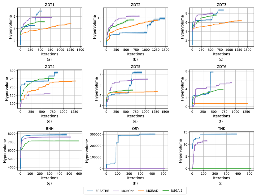
Figure 9. Convergence of hypervolume, when comparing BREATHE against baselines, on the (a-f) ZDT1-6 problem suite, (g) BNH, (h) OSY, and (i) TNK benchmarks. All methods were executed until convergence. For all plots, we show the mean and one standard error of the mean over five replications.

Fig. 9 shows the convergence of hypervolume with the number of algorithm iterations for BREATHE and baseline methods on benchmark applications. Here, we show the hypervolume that is dominated by the provided set of solutions with respect to a reference point (set by the maximum possible value of each output objective) (Fonseca et al., 2006). We observe that BREATHE outperforms baselines on most benchmarks (except ZDT2). MOEA/D does not support constraints and is therefore not plotted for BNH, OSY, and TNK tasks. Further, for the OSY task, NSGA-2 and MOBOpt could not find any legal inputs (that satisfy all constraints), resulting in the hypervolume being zero.

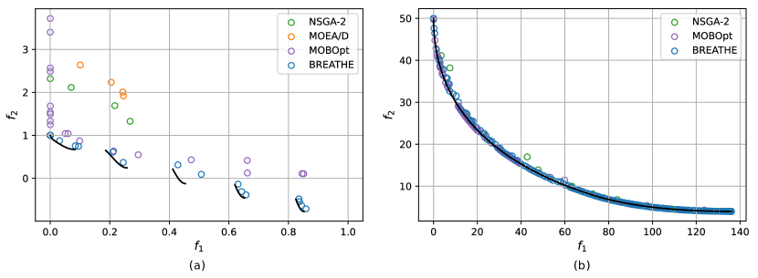
Figure 10. Pareto fronts obtained by various MOO methods on the (a) ZDT3 and (b) BNH tasks.

Fig. 10 shows the obtained Pareto fronts for the ZDT3 and BNH tasks. ZDT3 has a disjoint and non-convex Pareto front. Even though BREATHE uses a convex combination scalarization function [see Eq. (8)], which has been shown to not perform well for non-convex Pareto fronts (Chugh, 2020), it is able to obtain non-dominated solutions close to ZDT3’s Pareto front due to multiple random cold restarts in the optimization loop. In Fig. 10(b), we show that BREATHE is able to achieve a denser set of non-dominated solutions on the Pareto front relative to baselines.

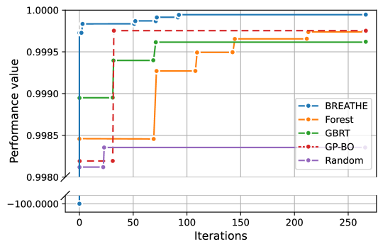
Figure 11. Performance convergence of BREATHE on the smart home application.

5.3. Searching for Optimal Graphs using BREATHE

We now run the G-BREATHE algorithm, as described in Section 3.2, for graph optimization. This implies searching for novel graphs along with node and edge weights that maximize the output performance measure $P$. Fig. 11 shows the convergence of $P$ with the number of iterations on the smart home task. This task has only one objective: minimization of the number of attacks. BREATHE outperforms all baselines. Even though randomly generated graphs may be legal in terms of the graph architecture, they may not honor all the constraints (for example, the number of windows should be greater than three). BREATHE and the baselines quickly find legal graphs (with $P\in[0,1]$). However, not being able to smartly search the graph architecture space limits the baselines from reaching the highest-achieved performance by BREATHE.

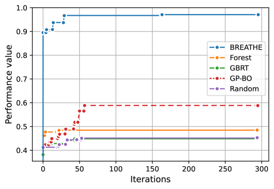
Figure 12. Performance convergence of BREATHE on the network application.

Fig. 12 shows the performance convergence for network optimization. This task has two objectives: maximization of the average bandwidth and minimization of overall network operation cost. The weights for the two objectives for the calculation of $P$ are 0.4 and 0.6, respectively. We choose these weights to attribute more importance to the network operation cost. A user can choose any set of weights that form a convex combination (as in Eq. (5)). Again, BREATHE outperforms baselines by achieving 64.9% higher performance than the next-best baselines, i.e., GP-BO (more details in Section 6).

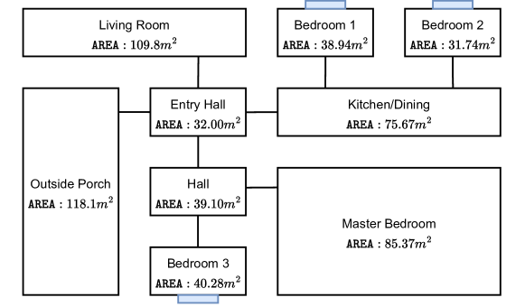
Figure 13. Best-performing smart home design that minimizes the number of cyber-physical attacks as per G-BREATHE.

Fig. 13 shows the obtained smart home design after running the BREATHE algorithm. All bedrooms have a window (shown by a blue box). Bedroom 1 has a WiFi modem and a smart thermostat. The entry hall contains an entry sensor, a smart door camera, and a smart lock at the door connecting to the outside porch. The kitchen/dining area has a home assistant and the master bedroom has a network gateway. Placing the gateway in a different room than the WiFi modem reduces the risk of attacks. Nevertheless, this design is prone to 65 physical (break-ins from the outside door or windows) and 92 cyber attacks (DDoS attacks affecting the gateway and, subsequently, the IoT devices). These correspond to different permutations of attacks one can perform. However, this is the least number of cyber-physical attacks achieved by the BREATHE algorithm.

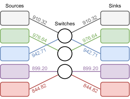
Figure 14. Best-performing network architecture that maximizes performance as per G-BREATHE. An annotation on a connection represents the bandwidth of that connection in MB/s.

Multiple network configurations lead to the same net performance value. For example, Fig. 14 shows one such best-performing network architecture. The cost of operation for the network is $35,457.37 and the average bandwidth is 914.74 MB/s. The network only uses three switches to minimize the base cost of setting them up. Two switches connect to two data source/sink pairs, while one switch connects to only one pair. We label these pairs and their corresponding connections in unique colors.

5.4. Ablation Analysis

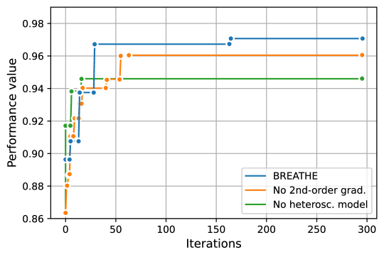
Figure 15. Ablation analysis of BREATHE on the network application.

We now present an ablation analysis of our proposed optimizer. Fig. 15 compares the performance convergence of BREATHE with that of its ablated versions. First, we remove second-order gradients ($\nabla^{2}_{x}$UCB) and implement GOBI with first-order gradients ($\nabla_{x}$UCB) instead. Second, we remove the NPN model, which models the aleatoric uncertainty (see Section 3.1). We can see that these changes result in poorer converged performance relative to the proposed BREATHE algorithm.

We now ablate the effect of the proposed legality-forcing method on benchmark applications with constraints. We present the results in Table 7. We observe that legality-forcing is crucial for constrained optimization. Without it, GOBI could result in inputs that are not legal.

Table 7. Effect of legality-forcing on constrained optimization using BREATHE.

Method	Application
	BNH	OSY	TNK
V-BREATHE	7894.4	301429.9	14.2
w/o legality-forcing	6933.5	-	7.8

5.5. Scalability Tests

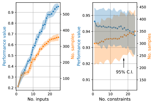
Figure 16. Effect of the number of (a) inputs and (b) constraints on the highest achieved performance value and the number of samples required to achieve it. BREATHE was executed on the SO-PWM task. Plotted with 95% confidence intervals.

We now test how scalable BREATHE is with the dimensionality of the optimization problem. Hence, we plot how the maximum achieved performance and the number of samples required to achieve that performance scale with an increasing number of inputs and constraints. Here, the number of samples corresponds to the total number of queries to the simulator. These include the seed samples required to initialize and train the surrogate model. To calculate the performance ($P$) on the SO-PWM task, we use $\alpha_{1}=\alpha_{2}=0.5$ to give equal weight to each objective. We show these plots in Fig. 16. First, we note that the maximum achieved performance scales linearly with the number of inputs and constraints. However, with increasing constraints, the maximum achieved performance value slowly decreases. Second, sample complexity scales sublinearly with the number of inputs and linearly with constraints.

6. Discussions and Limitations

Table 8. Summary of experimental results for various optimization applications. Best-achieved performance is reported for SOO tasks and the highest achieved hypervolume is reported for the MOO tasks. ^∗The graphical version of the baseline was implemented as described in Section 4.3.

SOO (Vector Optimization)
Application	Random	GP-BO	GBRT	Forest	V-BREATHE
Op-amp	-100.0	-100.0	0.9991	0.9997	0.9999
WWTP	0.2735	0.6517	0.4996	0.6006	0.9858
SOO (Graph Optimization)
Application	Random∗	GP-BO∗	GBRT∗	Forest∗	G-BREATHE
Smart Home	0.9983	0.9997	0.9996	0.9997	0.9999
Network	0.4512	0.5885	0.4482	0.4846	0.9707
MOO (Vector Optimization)
Application	NSGA-2	MOEA/D		MOBOpt	V-BREATHE
WWTP ($S_{I}$ vs. $S_{S}$)	39.4	67.6		263.9	5781.3
WWTP ($X_{I}$ vs. $X_{S}$)	3.2	182.3		150.2	3024.1
ZDT1	5.1	4.8		5.9	7.1
ZDT2	9.7	9.6		10.3	9.9
ZDT3	7.6	6.4		8.0	8.5
ZDT4	250.7	238.6		159.1	282.4
ZDT5	4.5	4.4		5.6	6.2
ZDT6	3.8	0.7		5.4	7.8
BNH	7137.2	-		7635.2	7894.4
OSY	-	-		-	301429.9
TNK	-	-		11.7	14.2

Table 8 summarizes the results presented in Section 5. The proposed framework outperforms baselines on various applications. In SOO, BREATHE achieves 64.1% higher performance than the next-best baseline, i.e., Forest on the WWTP application. G-BREATHE achieves 64.9% higher performance than the next-best baseline, i.e., a graphical version of GP-BO, on the network application. In MOO, BREATHE achieves up to 21.9$\times$ higher hypervolume relative to the next-best baseline, namely, MOBOpt (in the $S_{I}$ vs. $S_{S}$ trade-off). BREATHE also outperforms baselines on standard MOO benchmark applications, except ZDT2. ZDT2 and ZDT6 are MOO problems with non-convex Pareto fronts. However, ZDT6 has only 10 inputs, while ZDT2 has 30 inputs. This leads us to believe that BREATHE may not always outperform the baselines when the optimization problem is non-convex and has high input dimensionality.

Although the surrogate model that undergirds the V-BREATHE framework is similar to that of BOSHNAS (Tuli et al., 2023a), many novelties are proposed in this work. These include legality-forcing of gradients to allow queries to adhere to input constraints, penalization for output constraint violations, and support for multi-objective optimization (although, we leave the exploration of more complex constraint management methods, like probability of feasibility (Sohst et al., 2022), to future work). Moreover, BOSHNAS only works with vector input, while G-BREATHE optimizes for graph architectures. G-BREATHE does not convert the graph-based problem into a vector-based problem. Instead, it directly works on graphical input. It not only optimizes for the node/edge weight values (that could, in principle, be reduced to a vector optimization problem) but also searches for the best-performing graph architecture (node connections, i.e., new edges). Graph architecture optimization has not been implemented by any previously-proposed surrogate-based optimization method, to the best of our knowledge.

In the demonstrated results, we show that different extrema on the Pareto front result in designs that maximize one objective at the cost of others and BREATHE outputs all such extrema. G-BREATHE achieves high performance values in graph search, resulting in designs that optimize output objectives while honoring user-defined constraints. Unlike previous works, BREATHE is a unified framework that supports sample-efficient optimization in different input spaces (vector- or graph-based) and user-defined constraints. This work shows the applicability of BREATHE to diverse optimization problems and explores the novel domain of graph optimization for generic applications (beyond NAS). BREATHE also leverages an actively trained heteroscedastic model to minimize sample complexity.

In this work, we tested G-BREATHE on graphical spaces with up to 25 nodes. The proposed G-BREATHE framework is applicable to larger graphs as well. However, case studies involving larger and more complex graphs would require domain expertise and modifications to the optimization method for better-posed search. This is because larger graphs exponentially increase the size of the design space. Exploring such cases is part of future work.

BREATHE has several limitations. It only supports optimization of an application where the simulator gives an output for any legal queried input. However, in some cases, the queried simulator could result in erroneous output. BREATHE does not detect such outputs based on the distributions learned from other input/output pairs. Detecting such pairs falls under the scope of adversarial attack detection (Pang et al., 2018) and label noise detection (Northcutt et al., 2021; Yue and Jha, 2022). Moreover, its surrogate model does not work with partially-specified inputs.

7. Conclusion

In this work, we presented BREATHE, a vector-space and graph-space optimizer that efficiently searches the design space for constrained single- or multi-objective optimization applications. It leverages second-order gradients and actively trains a heteroscedastic model by iteratively querying an expensive simulator. BREATHE outperforms the next-best baseline, Forest, with up to 64.1% higher performance. G-BREATHE is an optimizer that efficiently searches for graphical architectures along with node and edge weights. It outperforms the next-best baseline, a graphical version of GP-BO, with up to 64.9% higher performance. Further, we leverage BREATHE for multi-objective optimization where it achieves up to 21.9$\times$ higher hypervolume than a state-of-the-art baseline, MOBOpt.

References

- (1)
- asc (2023) ASCO: A SPICE Circuit Optimizer. (2023). https://asco.sourceforge.net
- spe (2023) Spectre® Circuit Simulator Reference. (2023). http://www.ece.utep.edu/courses/web5369/Links_files/spectreuser_5.0.pdf
- zwa (2023) Z-Wave. (2023). https://www.z-wave.com
- zig (2023) Zigbee: The Full-stack Solution for all Smart Devices. (2023). https://csa-iot.org/all-solutions/zigbee/
- Applegate et al. (2011) David L. Applegate, Robert E. Bixby, Vašek Chvátal, and William J. Cook. 2011. The traveling salesman problem. In The Traveling Salesman Problem. Princeton University Press.
- Audet and Hare (2017) Charles Audet and Warren Hare. 2017. Derivative-free and Blackbox Optimization. Vol. 2. Springer.
- Bajaj et al. (2021) Ishan Bajaj, Akhil Arora, and M. M. Faruque Hasan. 2021. Black-Box Optimization: Methods and Applications. Springer International Publishing, 35–65.
- Binh and Korn (1997) To Thanh Binh and Ulrich Korn. 1997. MOBES: A multiobjective evolution strategy for constrained optimization problems. In Proc. Int. Conf. Genetic Algorithms, Vol. 25.
- Blank and Deb (2020) Julien Blank and Kalyanmoy Deb. PyMoo: Multi-objective optimization in Python. IEEE Access 8 (2020), 89497–89509.
- Buluç et al. (2016) Aydın Buluç, Henning Meyerhenke, Ilya Safro, Peter Sanders, and Christian Schulz. Recent advances in graph partitioning. Algorithm Engineering (2016), 117–158.
- Chen et al. (1985) Kueing-Long Chen, Stephen A. Saller, Imelda A. Groves, and David B. Scott. Reliability effects on MOS transistors due to hot-carrier injection. IEEE Trans. Electron Devices 32, 2 (1985), 386–393.
- Chugh (2020) Tinkle Chugh. 2020. Scalarizing functions in Bayesian multiobjective optimization. In Proc. IEEE Congress on Evolutionary Computation. IEEE, 1–8.
- Chugh et al. (2019) Tinkle Chugh, Karthik Sindhya, Jussi Hakanen, and Kaisa Miettinen. A survey on handling computationally expensive multiobjective optimization problems with evolutionary algorithms. Soft Computing 23 (2019), 3137–3166.
- Daulton et al. (2022) Samuel Daulton, David Eriksson, Maximilian Balandat, and Eytan Bakshy. 2022. Multi-objective Bayesian optimization over high-dimensional search spaces. In Proc. Int. Conf. Uncertainty in Artificial Intelligence, Vol. 180. 507–517.
- De Ath et al. (2021) George De Ath, Richard M. Everson, and Jonathan E. Fieldsend. 2021. Asynchronous \textepsilon-greedy Bayesian optimisation. In Proc. Conf. Uncertainty in Artificial Intelligence, Vol. 161. 578–588.
- Deb (2011) Kalyanmoy Deb. 2011. Multi-objective optimisation using evolutionary algorithms: An introduction. In Multi-objective Evolutionary Optimisation for Product Design and Manufacturing. Springer, 3–34.
- Deb et al. (2002) Kalyanmoy Deb, Amrit Pratap, Sameer Agarwal, and Thirunavukarasu Meyarivan. A fast and elitist multiobjective genetic algorithm: NSGA-II. IEEE Trans. Evolutionary Computation 6, 2 (2002), 182–197.
- Draine (2010) Bruce T. Draine. 2010. Physics of the Interstellar and Intergalactic Medium. Princeton University Press.
- Emmerich and Deutz (2018) Michael T. M. Emmerich and André H. Deutz. A tutorial on multiobjective optimization: Fundamentals and evolutionary methods. Natural Computing 17 (2018), 585–609.
- Eschauzier and Huijsing (1995) Rudy G. H. Eschauzier and Johan Huijsing. 1995. Frequency Compensation Techniques for Low-power Operational Amplifiers. Vol. 313. Springer Science & Business Media.
- Esfahani et al. (2018) Ehsan Banayan Esfahani, Fatemeh Asadi Zeidabadi, Alireza Bazargan, and Gordon McKay. The modified Bardenpho process. Handbook of Environmental Materials Management (2018), 1–50.
- Fonseca et al. (2006) Carlos M. Fonseca, Luís Paquete, and Manuel López-Ibánez. 2006. An improved dimension-sweep algorithm for the hypervolume indicator. In Proc. IEEE Int. Conf. Evolutionary Computation. 1157–1163.
- Galuzio et al. (2020) Paulo Paneque Galuzio, Emerson Hochsteiner de Vasconcelos Segundo, Leandro dos Santos Coelho, and Viviana Cocco Mariani. MOBOpt — multi-objective Bayesian optimization. SoftwareX 12 (2020), 100520.
- Geifman and El-Yaniv (2018) Yonatan Geifman and Ran El-Yaniv. Deep active learning with a neural architecture search. CoRR abs/1811.07579 (2018).
- Gill et al. (2019) Sukhpal Singh Gill, Shreshth Tuli, Minxian Xu, Inderpreet Singh, Karan Vijay Singh, Dominic Lindsay, Shikhar Tuli, Daria Smirnova, Manmeet Singh, Udit Jain, Haris Pervaiz, Bhanu Sehgal, Sukhwinder Singh Kaila, Sanjay Misra, Mohammad Sadegh Aslanpour, Harshit Mehta, Vlado Stankovski, and Peter Garraghan. Transformative effects of IoT, blockchain and artificial intelligence on cloud computing: Evolution, vision, trends and open challenges. Internet of Things 8 (2019), 100–118.
- Gupta et al. (2020) Charu Gupta, Anshul Gupta, Shikhar Tuli, Erik Bury, Bertrand Parvais, and Abhisek Dixit. Characterization and modeling of hot carrier degradation in n-channel gate-all-around nanowire FETs. IEEE Trans. Electron Devices 67, 1 (2020), 4–10.
- Jensen and Toft (2011) Tommy R Jensen and Bjarne Toft. 2011. Graph Coloring Problems. John Wiley & Sons.
- Ke et al. (2017) Guolin Ke, Qi Meng, Thomas Finley, Taifeng Wang, Wei Chen, Weidong Ma, Qiwei Ye, and Tie-Yan Liu. 2017. LightGBM: A highly efficient gradient boosting decision tree. In Proc. Int. Conf. Neural Information Processing Systems, Vol. 30. 3149–3157.
- Krajzewicz et al. (2012) Daniel Krajzewicz, Jakob Erdmann, Michael Behrisch, and Laura Bieker. Recent development and applications of SUMO-simulation of urban mobility. Int. J. Advances in Systems and Measurements 5, 3&4 (2012).
- Kumar et al. (2021) Abhishek Kumar, Guohua Wu, Mostafa Z. Ali, Qizhang Luo, Rammohan Mallipeddi, Ponnuthurai Nagaratnam Suganthan, and Swagatam Das. A benchmark-suite of real-world constrained multi-objective optimization problems and some baseline results. Swarm and Evolutionary Computation 67 (2021), 100961.
- Leighton and Rao (1999) Tom Leighton and Satish Rao. Multicommodity max-flow min-cut theorems and their use in designing approximation algorithms. J. ACM 46, 6 (1999), 787–832.
- Liu and Nocedal (1989) Dong C. Liu and Jorge Nocedal. On the limited memory BFGS method for large scale optimization. Mathematical Programming 45, 1 (1989), 503–528.
- Liu et al. (2019) Hanxiao Liu, Karen Simonyan, and Yiming Yang. 2019. DARTS: Differentiable architecture search. In Proc. Int. Conf. Learning Representations.
- Niederreiter (1992) Harald Niederreiter. 1992. Random Number Generation and Quasi-Monte Carlo Methods. SIAM.
- Northcutt et al. (2021) Curtis Northcutt, Lu Jiang, and Isaac Chuang. Confident learning: Estimating uncertainty in dataset labels. J. Artificial Intelligence Research 70 (2021), 1373–1411.
- Osyczka and Kundu (1995) Andrzej Osyczka and Sourav Kundu. A new method to solve generalized multicriteria optimization problems using the simple genetic algorithm. Structural Optimization 10 (1995), 94–99.
- Pang et al. (2018) Tianyu Pang, Chao Du, Yinpeng Dong, and Jun Zhu. 2018. Towards robust detection of adversarial examples. In Proc. Int. Conf. Neural Information Processing Systems, Vol. 31.
- Pedregosa et al. (2011) Fabian Pedregosa, Gaël Varoquaux, Alexandre Gramfort, Vincent Michel, Bertrand Thirion, Olivier Grisel, Mathieu Blondel, Peter Prettenhofer, Ron Weiss, Vincent Dubourg, Jake Vanderplas, Alexandre Passos, David Cournapeau, Matthieu Brucher, Matthieu Perrot, and Édouard Duchesnay. Scikit-learn: Machine learning in Python. J. Machine Learning Research 12 (2011), 2825–2830.
- Rahi et al. (2022) Kamrul Hasan Rahi, Hemant Kumar Singh, and Tapabrata Ray. A steady-state algorithm for solving expensive multi-objective optimization problems with non-parallelizable evaluations. IEEE Trans. Evolutionary Computation (2022). https://doi.org/10.1109/TEVC.2022.3219062 (Early Access).
- Rathore et al. (2010) Akshay K. Rathore, Joachim Holtz, and Till Boller. Synchronous optimal pulsewidth modulation for low-switching-frequency control of medium-voltage multilevel inverters. IEEE Trans. Industrial Electronics 57, 7 (2010), 2374–2381.
- Ren et al. (2021) Pengzhen Ren, Yun Xiao, Xiaojun Chang, Po-Yao Huang, Zhihui Li, Brij B. Gupta, Xiaojiang Chen, and Xin Wang. A survey of deep active learning. ACM Comput. Surv. 54, 9, Article 180 (2021), 40 pages.
- Rogers et al. (2019) Keir K. Rogers, Hiranya V. Peiris, Andrew Pontzen, Simeon Bird, Licia Verde, and Andreu Font-Ribera. Bayesian emulator optimisation for cosmology: Application to the Lyman-alpha forest. Journal of Cosmology and Astroparticle Physics 2019, 02 (2019).
- Shi et al. (2021) Yunsheng Shi, Zhengjie Huang, Shikun Feng, Hui Zhong, Wenjing Wang, and Yu Sun. 2021. Masked label prediction: Unified message passing model for semi-supervised classification. In Proc. Int. Conf. Artificial Intelligence. 1548–1554.
- Siddiqi (2021) Irfan Siddiqi. Engineering high-coherence superconducting qubits. Nature Reviews Materials 6, 10 (2021), 875–891.
- Snoek et al. (2012) Jasper Snoek, Hugo Larochelle, and Ryan P. Adams. 2012. Practical Bayesian optimization of machine learning algorithms. In Proc. Int. Conf. Neural Information Processing Systems, Vol. 25. 2951–2959.
- Sohst et al. (2022) Martin Sohst, Frederico Afonso, and Afzal Suleman. Surrogate-based optimization based on the probability of feasibility. Structural and Multidisciplinary Optimization 65, 1 (2022).
- Tanaka et al. (1995) Masahiro Tanaka, Hikaru Watanabe, Yasuyuki Furukawa, and Tetsuzo Tanino. 1995. GA-based decision support system for multicriteria optimization. In Proc. IEEE Int. Conf. Systems, Man and Cybernetics, Vol. 2. 1556–1561.
- Terway et al. (2022) Prerit Terway, Kenza Hamidouche, and Niraj K. Jha. Fast design space exploration of nonlinear systems: Part II. IEEE Trans. Computer-Aided Design of Integrated Circuits and Systems 41, 9 (2022), 2984–2999.
- Tuli et al. (2023a) Shikhar Tuli, Bhishma Dedhia, Shreshth Tuli, and Niraj K. Jha. FlexiBERT: Are current transformer architectures too homogeneous and rigid? J. Artificial Intelligence Research 7 (2023), 39–70.
- Tuli and Jha (2023) Shikhar Tuli and Niraj K. Jha. Edgetran: Co-designing transformers for efficient inference on mobile edge platforms. CoRR abs/2303.13745 (2023).
- Tuli et al. (2023b) Shikhar Tuli, Chia-Hao Li, Ritvik Sharma, and Niraj K. Jha. CODEBench: A neural architecture and hardware accelerator co-design framework. ACM Trans. Embed. Comput. Syst. 22, 3, Article 51 (2023), 30 pages.
- Tuli et al. (2021) Shreshth Tuli, Shivananda R. Poojara, Satish N. Srirama, Giuliano Casale, and Nicholas R. Jennings. COSCO: Container orchestration using co-simulation and gradient based optimization for fog computing environments. IEEE Trans. Parallel and Distributed Systems 33, 1 (2021), 101–116.
- Wang et al. (2016) Hao Wang, Xingjian Shi, and Dit-Yan Yeung. 2016. Natural-parameter networks: A class of probabilistic neural networks. In Proc. Int. Conf. Neural Information Processing Systems. 118–126.
- Yue and Jha (2022) Chang Yue and Niraj K. Jha. CTRL: Clustering training losses for label error detection. CoRR abs/2208.08464 (2022).
- Zhang and Li (2007) Qingfu Zhang and Hui Li. MOEA/D: A multiobjective evolutionary algorithm based on decomposition. IEEE Trans. Evolutionary Computation 11, 6 (2007), 712–731.
- Zitzler et al. (2000) Eckart Zitzler, Kalyanmoy Deb, and Lothar Thiele. Comparison of multiobjective evolutionary algorithms: Empirical results. Evol. Comput. 8, 2 (2000), 173–195.