The galactic acceleration scale is imprinted on globular cluster systems of early-type galaxies of most masses and on red and blue globular cluster subpopulations

Abstract

Context. Globular clusters (GCs) carry information about the formation histories and gravitational fields of their host galaxies. Bílek et al. (2019, BSR19 hereafter) reported that the radial profiles of the volume number density of GCs in GC systems (GCSs) follow broken power laws, while the breaks occur approximately at the $a_{0}$ radii. These are the radii at which the gravitational fields of the galaxies equal the galactic acceleration scale $a_{0}=1.2\times 10^{-10}\,$m s${}^{-2}$ known from the radial acceleration relation or the MOND theory of modified dynamics.

Aims. Our main goals here are to explore whether the results of BSR19 hold true for galaxies of a wider mass range and for the red and blue GC subpopulations.

Methods. We exploited catalogs of photometric GC candidates in the Fornax galaxy cluster based on ground and space observations and a new catalog of spectroscopic GCs of NGC 1399, the central galaxy of the cluster. For every galaxy, we obtained the parameters of the broken power-law density by fitting the on-sky distribution of the GC candidates, while allowing for a constant density of contaminants. The logarithmic stellar masses of our galaxy sample span $8.0-11.4\,M_{\sun}$.

Results. All investigated GCSs with a sufficient number of members show broken power-law density profiles. This holds true for the total GC population and the blue and red subpopulations. The inner and outer slopes and the break radii agree well for the different GC populations. The break radii agree with the $a_{0}$ radii typically within a factor of two for all GC color subpopulations. The outer slopes correlate better with the $a_{0}$ radii than with the galactic stellar masses. The break radii of NGC 1399 vary in azimuth, such that they are greater toward and against the direction to NGC 1404, which tidally interacts with NGC 1399.

1 Introduction

Globular clusters (GCs) are compact (a few parsecs), massive ($10^{4}-10^{6}\,M_{\sun}$) star systems found in nearly all galaxies. A galaxy similar to the Milky Way has a few hundreds of them, while giant ellipticals can have more than ten thousand GCs. The colors of many galaxies form a bimodal distribution, with rather universal positions for the two peaks. Therefore, GCs are divided into two types – the metal-poor “blue GCs” and the metal-rich “red GCs” (Brodie2006; cantiello20). Red GCs generally follow the kinematics of the stars in a galaxy, with a similar rotational velocity and velocity dispersion. In contrast, blue GCs often show complex kinematics (schuberth10; Coccato2013; Chaturvedi22). The spatial distribution of GCs around galaxies is more centrally concentrated for the red GCs than for the blue GCs. The distinct properties of the red and blue GCs point toward their different formation pathways (ashman95; peng06; Brodie2006). It seems that the blue GCs are added to massive galaxies via accretion of low-mass galaxies, while most red GCs form in situ, together with the stars of the host galaxy (cote98; harrissaasfee; tonini13; renaud17). Globular cluster systems thus carry information about the assembly history of their host galaxies (Peng2008; Brodie2014; Harris2016). The number of GCs that a galaxy hosts is proportional to the expected mass of its dark matter halo (spitler09; harris15). The kinematics and distribution of GC systems (GCSs) reflect the profiles of the gravitational fields of their host galaxies (samur14; samur16; alabi17; bil19).

In the paper by bil19b (BSR19 hereafter), an interesting new property of GCSs of early-type galaxies was noted. They parametrized the volume number density of GCs in a GCS, $\rho$ by a broken power law as

$$\rho(r) =\rho_{0}\ r^{a} \quad\textrm{ for }\quad r<r_{\mathrm{br}},$$ (1)

$$\rho(r) =\rho_{0}\ r_{\mathrm{br}}^{a-b}\ r^{b} \quad\textrm{ for }\quad r\geq r_{\mathrm{br}},$$

where $r$ is the galactocentric radius. The parameter $r_{\mathrm{br}}$ was called the break radius. The authors found that the break radius coincides well with the $a_{0}$ radius, that is the radius at which the expected gravitational acceleration generated by the baryons of the galaxy equals the galactic acceleration scale $a_{0}=1.2\times 10^{-10}\,$m s${}^{-2}$. The values of the break radii did not agree with the values of the other characteristic lengths of the galaxies, such as stellar effective radii or dark halo scale radii. These other lengths were either several times bigger or smaller than the break radii, at least for a substantial fraction of the galaxy sample (see their Table 1).

The galactic acceleration scale is known best from the behavior of the observed gravitational fields of galaxies (e.g., lelli17; li17). In the regions of galaxies where the gravitational acceleration expected by Newtonian gravity from the distribution of baryons $g_{\mathrm{N}}$ is greater than $a_{0}$, the observed gravitation acceleration equals $g_{\mathrm{N}}$, meaning that the Newtonian dynamics does not require dark matter. On the other hand, in the regions where $g_{\mathrm{N}}$ is lower than $a_{0}$, the observed gravitational acceleration is very close to $\sqrt{g_{\mathrm{N}}a_{0}}$. The same rules apply even for many, or perhaps all, GCs (scarpa10; scarpa11; ibata11; sanders12; hernandez12; hernandez20).

This behavior was initially predicted by the modified Newtonian dynamics (MOND), which is a class of modified gravity and inertia theories (milg83a). Here we assume MOND to be a modified gravity theory. It predicts that the gravitational acceleration in spherical isolated objects is (milg83a; qumond; famaey12)

$$g_{\mathrm{M}}=g_{\mathrm{N}}\,\nu(g_{\mathrm{N}}/a_{0}).$$ (2)

The function $\nu$ is not known exactly, but it must have the limit behavior $\nu(x)\sim x^{-1/2}$ for $x\ll 1$, and $\nu(x)\sim 1$ for $x\gg 1$. This gives rise to two regimes of a gravitational field around a galaxy: the strong field, the so-called Newtonian regime, and the weak field, the so-called deep-MOND regime. The observed counterpart of Eq. 2 is known as the radial acceleration relation (mcgaugh16).

Apart from the radial acceleration relation, MOND predicted or explained many other observational laws (milg83a; milg83b; milg83c), all of which contain the constant $a_{0}$. This is the case for the baryonic Tully-Fisher relation (mcgaugh20; lelli19), the Faber-Jackson relation (faber76; famaey12), and the radial acceleration relation, which connect the mass or mass distribution of galaxies to the velocities of stars and gas in them. The Fish law (fish64; allen79) and Freeman limit (freeman70; mcgaugh95; fathi10; famaey12) give upper limits on the surface brightness for elliptical and spiral galaxies, respectively, above which galaxies are rare. Recently, there appeared a MOND explanation (milg21) of the Fall relation (fall83; posti18), which connects the mass and specific angular momentum of galaxies. The law of the universal surface density of the cores of the putative dark matter halos (kormendy04; donato09; salucci12) can be explained by MOND as well (milg09c).

Finally, there are interesting numerical coincidences of $a_{0}$ with the constants of cosmology (milg83a; milg20). If we denote $H_{0}$ the Hubble constant, $c$ the speed of light, $G$ the gravitational constant, $R_{H}$ the size of the cosmic horizon, and $M_{H}$ the total mass inside the cosmic horizon, then we find the order-of-magnitude equalities $a_{0}\approx cH_{0}\approx c^{2}\Lambda^{1/2}\approx c^{2}/R_{H}\approx c^{4}/GM_{H}$. There is no clear explanation of these coincidences yet (navarro17; milg20).

The finding of BSR19, of the equality of the break and $a_{0}$ radii, is thus another case of the many occurrences of the constant $a_{0}$ in extragalactic astronomy. More precisely, in this work we consider two types of $a_{0}$ radii: i) the one where the acceleration calculated from the distribution of baryons and Newtonian gravity equals $a_{0}$ and ii) where the acceleration calculated for MOND gravity via Eq. 2 equals $a_{0}$. For most galaxies, the two $a_{0}$ radii are numerically similar. Therefore, in this paper, if we do not specify whether we are referring to Newtonian or MOND $a_{0}$, then we mean that the statement is valid for both options.

Table 1: Parameters of the investigated galaxies.

Name	FDS ID	$\log_{10}\frac{M_{*}}{M_{\sun}}$	$R_{\mathrm{e}}$	$n$	$r_{\!a_{0}\mathrm{,M}}$	$r_{\!a_{0}\mathrm{,N}}$
			[arcmin]		[kpc]	[kpc]
ESO358-006	FDS19_0001	$9.40\pm 0.09$	0.25	1.1	$1.44^{+0.5}_{\mbox{\leavevmode\nobreak\ \leavevmode\nobreak\ --}}$	–
ESO358-050	FDS4_0001	$9.5\pm 0.1$	0.32	1.8	$1.50^{+0.4}_{-0.4}$	$0.43^{+0.3}_{\mbox{\leavevmode\nobreak\ \leavevmode\nobreak\ --}}$
NGC1316	FDS26_0001	$11.40\pm 0.06$	1.0	4.3	$21.5^{+2}_{-2}$	$14.3^{+1}_{-1}$
NGC1336	FDS20_0000	$9.7\pm 0.1$	0.70	4.6	$1.63^{+0.3}_{-0.3}$	$0.89^{+0.2}_{-0.2}$
NGC1351	FDS19_0000	$10.30\pm 0.07$	0.75	5.9	$4.65^{+0.5}_{-0.5}$	$2.91^{+0.3}_{-0.3}$
NGC1373	FDS16_0002	$9.40\pm 0.09$	0.16	3.9	$1.95^{+0.3}_{-0.3}$	$1.24^{+0.2}_{-0.2}$
NGC1379	FDS11_0002	$10.40\pm 0.06$	0.47	2.7	$6.57^{+0.7}_{-0.6}$	$4.11^{+0.5}_{-0.4}$
NGC1380	FDS11_0006	$10.90\pm 0.05$	0.77	3.0	$11.79^{+0.9}_{-0.9}$	$7.51^{+0.7}_{-0.6}$
NGC1380B	FDS11_0005	$9.7\pm 0.1$	0.28	1.9	$2.65^{+0.5}_{-0.5}$	$1.40^{+0.4}_{-0.3}$
NGC1381	FDS11_0004	$10.20\pm 0.07$	0.31	2.6	$5.48^{+0.6}_{-0.5}$	$3.53^{+0.4}_{-0.4}$
NGC1387	FDS11_0001	$10.70\pm 0.05$	0.61	5.5	$8.90^{+0.7}_{-0.6}$	$5.84^{+0.5}_{-0.4}$
NGC1399	FDS11_0003	$11.40\pm 0.06$	2.6	8.1	$16.9^{+2}_{-1}$	$10.9^{+1}_{-1}$
NGC1404	FDS11_0166	$11.00\pm 0.06$	0.54	4.0	$14.1^{+1}_{-1}$	$9.49^{+0.8}_{-0.7}$
NGC1419	FDS13_0000	$9.90\pm 0.09$	0.16	4.0	$3.96^{+0.5}_{-0.5}$	$2.65^{+0.4}_{-0.3}$
NGC1427	FDS6_0001	$10.50\pm 0.06$	0.83	5.0	$6.11^{+0.6}_{-0.5}$	$3.80^{+0.4}_{-0.4}$
NGC1428	FDS6_0002	$9.6\pm 0.1$	0.19	1.7	$2.72^{+0.4}_{-0.4}$	$1.64^{+0.3}_{-0.3}$
Stack_8.0	–	$8.0\pm 0.1$	0.24	1.1	–	–
Stack_8.5	–	$8.40\pm 0.08$	0.23	1.3	–	–
Stack_9.0	–	$9.00\pm 0.08$	0.26	2.0	$0.36^{+0.2}_{-0.2}$	–

The theoretical explanation for why the $a_{0}$ radii coincide with the break radii of GCSs has not been clarified yet, even if some initial proposal were given in BSR19. Importantly, according to one of the proposed explanations that involves the Newtonian gravity and dark matter, the match of the $a_{0}$ and break radii is of practical importance. It had been found before that the number of GCs that a galaxy has is proportional to the mass of its dark matter halo (spitler09; harris15). The new finding allows one to estimate the scale radius of the halo: the break radius should be located at the radius where the gravitational attraction of the stars of the galaxy equals that of the dark matter halo. One can thus solve the equation of the equity of the accelerations to obtain the scale radius of the halo.

The paper BRS19 left several important questions open, which we aim to answer here. We investigate the distribution of GCs primarily using photometric data for early-type galaxies in the Fornax galaxy cluster, but we also analyze new spectroscopic data for two galaxies. The galaxy sample of BSR19 spanned only about one order of magnitude in stellar mass. The data investigated here allow us to verify that the match between the $a_{0}$ and break radii holds true for early-type galaxies spanning three orders of magnitude – from dwarfs of the mass of the Magellanic clouds to the brightest cluster galaxies. The distribution of GCs was investigated in BSR19 on the basis of the catalog of spectroscopically confirmed GCs. This approach can lead to distorted results, because spectroscopic surveys usually are spatially incomplete. This could have affected the derived parameters of the broken power-law profile. The verification of the match of the $a_{0}$ and break radii in the new data thus removes the shade of doubt that was left about the results of the previous work. The data in BSR19 do not allow the density profiles of the red and blue GC subpopulations to be investigated. We do this here and find that there are no statistically significant trends of the profile parameters with the color of the GCs. We exploit the new data for a further exploration of the profiles of GCSs. In particular, we investigate whether the parameters of the broken power-law profiles correlate with each other and with the parameters of the host galaxy. We also investigate in detail the GCS of NGC 1399, that is the central galaxy of the Fornax cluster. We find that its break radius depends on the relative velocity of the GCs with respect to the center of the galaxy, and that the break radius varies as a function of the position angle. In this paper, we also aim to explain the reason of why the GCSs of our galaxies have the broken power-law density profiles and why the break radii coincide with the $a_{0}$ radii. Several explanations were proposed in BSR19, and here we add a few more. Then we make the first steps toward finding which of them is correct. None seem perfect at this point.

This paper is organized as follows. In Sect. 2 we describe the observational data that we analyze here. The methods to extract and fit the radial profiles of volume number densities of GCs in the GCSs of the investigated galaxies are detailed in Sect. 3. The derivation of the $a_{0}$ radii for our sample galaxies is explained in Sect. LABEL:sec:ao. We present our results in Sect. LABEL:sec:results. In particular, in Sect. LABEL:sec:colors we compare the structural parameters of GCSs for the total GC population and the red and blue subpopulations. In Sect. LABEL:sec:corr we investigate the correlations of the structural parameters between each other and with the characteristics of the host galaxies and, finally, we explore the relation between the break and $a_{0}$ radii in Sect. LABEL:sec:equality. We explore the details of the distribution of GCs of NGC 1399 in Sect. LABEL:sec:n1399. We explore the credibility of some potential explanations of the approximate coincidence of the $a_{0}$ and break radii in Sect. LABEL:sec:interpretation. Finally we synthesize and summarize our findings in Sect. LABEL:sec:sum. In this work, we denote the natural logarithm by $\log$ and the logarithm of the base $m$ by $\log_{m}$. We assume the distance of the Fornax cluster and all the investigated galaxies to be 20.0 Mpc (blakeslee09). This corresponds to the angular scale of 5.8 kpc per arcminute.

2 Data analyzed

The galaxies investigated in this paper are member galaxies of the Fornax galaxy cluster. They are listed in Table 1. Low-mass Fornax cluster galaxies ($M_{*}<10^{9.5}M_{\sun}$) have too few GCs for constructing the density profiles of their GCSs individually. Therefore, we stacked the GC candidatess of many low-mass galaxies in three mass bins in order to get their average GCS density profiles. These are the three “Stack” entries in Table 1. The details of the stacking procedure are explained in Sect. 2.3.

All structural parameters of the galaxies in Table 1 were taken from su21. They are based on GALFIT profile fitting (penggalfit), using Sérsic functions, to photometric $g^{\prime}$-band data of the Fornax Deep Survey (FDS) (iodice16; venhola18). Stellar masses also come from that work. They were derived from empirical relations between colors and stellar mass-to-light ratio. We use archival photometric and spectroscopic catalogs of GC candidates for investigating their spatial distribution. Here follows a brief description of the datasets investigated in our work.

2.1 ACS Fornax cluster survey data

The ACS Fornax cluster survey (ACSFCS), taken using the Advanced Camera for Surveys (ACS) of the Hubble Space Telescope (HST), imaged 43 early-type galaxies of the Fornax cluster. Full details of the ACSFCS, scientific motivations and data reduction techniques, are given in jordan07. Each galaxy in ACSFCS was imaged in the F475W ($g$) and F850LP ($z$) bands. For studying the GCs, each image was sufficiently deep such that 90% of the GCs within the ACS FOV can be detected. The selection and identification of bonafide GCs of the ACSFCS galaxies are performed in the size-magnitude plane (jordan15). The resulting catalog of GCs in the ACSFCS provides the probability of an object being a GC, denoted by Pgcs, where Pgcs is a function of half-light radius, apparent magnitude and local background. For our analysis, we selected GCs with Pgcs larger than 0.5. This leaves the faintest GC candidates of $m_{g}=26.3$ mag. To separate the GCs into red and blue subpopulations, we adopted a dividing $g-z$ color of 1.1 mag (fahrion20).

2.2 Spectroscopically confirmed GCs

We studied the spectroscopically confirmed sample of GCs of the Fornax cluster from the recent catalog produced by Chaturvedi22. Reanalyzing data of the Fornax cluster taken using the Visible Multi-Object Spectrograph (VIMOS) at the Very Large Telescope (VLT) (pota18) and adding literature work, they have produced the most extensive GC radial velocity catalog of the Fornax cluster (see Chaturvedi22, for details), comprising more than 2300 confirmed GCs. The faintest GC has $m_{g}=24.2$ mag. They used a Gaussian modeling mixture technique to divide the GC population into red and blue GCs, with $g-i\sim 1.0$ mag as separating color, which we adopt in our analysis.

2.3 Fornax Deep Survey data

The Fornax Deep Survey (FDS) is a joint project based on a guaranteed time observation of the FOCUS (P.I. R. Peletier) and VEGAS (P.I. E. Iodice, Capaccioli15) surveys. It consists of deep multiband ($u$, $g$, $r$ and $i$ ) imaging data from OmegaCAM at the VST (kuijken11; Schipani12) and covers an area of 30 square degrees out to the virial radius of the Fornax cluster.

We applied morphological and photometric selection criteria to the photometric compact sources catalog of the FDS (cantiello20) to decrease the fraction of contaminant objects that are not GCs. The criteria on the colors of the selected objects $g-i>0.5$ and $g-i<1.6$ were chosen according to the colors of spectroscopically confirmed GCs around the central cluster galaxy NGC 1399. Further criteria were inspired by cross-matching the FDS and ACS catalogs of GCs of NGC 1399. They were chosen such that we do not exclude too many real GCs and, at the same time, exclude as many contaminants as possible. We found a good balance when using the following criteria: CLASS_STAR¿0.031, $m_{g}>20$ mag, and Elongation¡3. The meaning of the parameters is explained in cantiello20. After applying the selection criteria, the faintest GC candidate in this calatog has $m_{g}=27.0$ mag.

It turned out that the FDS catalog, after applying the GC candidate selection criteria, shows systematic variations of the surface density of sources that have a tile-like pattern, see Fig. 1. The tiles corresponds to the OmegaCAM imaging tiles of the FDS survey. They probably result from varying observing conditions, like seeing, sky transparency, etc. When fitting the surface density profiles of GCSs of individual galaxies, we had to be careful that the tile borders do not introduce any kinks in the profiles. We did this first by visual inspection of plots of positions of the GC candidates in the wide neighborhood of the investigated galaxies and second by visual inspection of the plots of the radial profiles of density of the GC candidates around the target galaxies.

2.3.1 Stacking of faint galaxies

As mentioned above, we decided to stack the faint galaxies of similar stellar mass in order to have enough sources to extract the density profiles of their GCSs. We used only the FDS data for this, since most faint galaxies were not covered by the ACSFCS. If the hypothesis of this paper, that the break radii coincide with the acceleration radii, is correct, then the break radii of all GCSs stacked in this way should be roughly equal in each mass bin (an acceleration radius nevertheless depends also on the particular distribution of mass in the given galaxy). We then treated the stacks as single galaxies. We created three such artificial objects. Their logarithmic masses were centered on the values of 8.0, 8.5 and 9.0 $M_{\sun}$. The widths of all logarithmic mass bins were 0.5 $M_{\sun}$. Stacking of galaxies of even lower masses did not provide sufficiently clear profiles of the projected density of GCs.

We stacked all galaxies from the su21 catalog that met the following criteria. First we excluded spiral galaxies, because our data do not allow to distinguish between GCs and star forming clumps or young star clusters in their disks. Early-type galaxies were identified by requiring their asymmetry parameter, stated in su21, to be lower than 0.06. We further excluded galaxies that are located close to the borders of the tiles of the FDS mosaic, and galaxies whose GCSs surface density profiles might be affected by interloping GCSs of other nearby galaxies. These were identified by visual inspection of the positions of the GC candidates in the neighborhood of the galaxies being stacked. The list of stacked objects in every mass bin is stated in Table LABEL:tab:fits in Appendix LABEL:app:fits.

We assigned to every stacked galaxy a stellar mass and Sérsic parameters. These were obtained as the median values for all galaxies included in the corresponding stack.

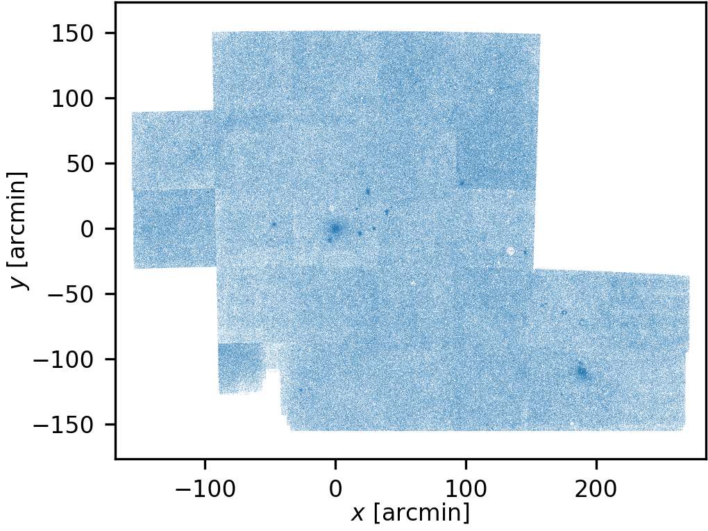
Figure 1: Positions of GC candidates in the FDS catalog, after applying selection criteria. The coordinate system is centered on NGC 1399. North is up, and west is to the right.

3 Fitting the surface density profiles of the GCSs by analytic functions

Here we describe how we determined for the investigated galaxies the parameters of the GCSs density profiles.

3.1 Extracting the observed profiles of surface density

For a given galaxy, we divided the GC candidates in radial bins according to their galactocentric distance, and for each bin, we calculated the surface density of sources in it. The bins had the shape of circular annuli, that is we ignored the possible ellipticity of the GCSs. We demonstrate in Appendix LABEL:app:ellipticity that this simplification has no appreciable impact on the derived profile of the GCS density. We chose the widths of the radial bins such that

$$N=n-A\overline{\gamma}$$ (3)

was constant in each bin. Here $n$ stands for the total number of sources falling in the annulus, $A$ the area of the annulus and $\overline{\gamma}$ an estimate of the surface density of contaminants. The number $N$ is thus the estimate of the number of GCs in the aperture. The parameter $N$ was chosen to be big enough so that the profile did not appear too noisy (as judged by eye) and small enough so that the two straight parts of the broken power law profile were resolved by at least three data points. The purpose of subtracting the expected number of contaminants was to increase the signal to noise in the outer bins. This condition was used only for choosing the bin widths; the final profile parameters of the GCSs (including the contaminants level) were derived from fitting the surface density of all sources, that is $n$.

For the datasets that are not expected to contain many contaminants, that is the spectroscopic and ACS catalogs, we used simply $\overline{\gamma}=0$. Otherwise the value of $\overline{\gamma}$ was found iteratively in the following way. We first chose a low value of $\overline{\gamma}$ and constructed the observed surface density profile. That was then fitted by some of the analytic model profiles described below. One of the parameters of the fitted profile was the density of the background sources, $\gamma$. In the next iteration we used a value of $\overline{\gamma}$ that lied between the value of $\overline{\gamma}$ used in the previous iteration and the fitted value of $\gamma$. We had to stop increasing $\overline{\gamma}$ at some point, because when it is too large, the extracted surface density profile would be truncated or distorted, because the expression on the right-hand-side of the condition Eq. 3 would be lower than the assigned value of $N$ at large radii. In some cases, the final $\overline{\gamma}$ was chosen such that the extracted profile did not show any small bumps arising from small clusters of contaminants (e.g., distant galaxy clusters in the background). We note that if the definitive $\overline{\gamma}$ was chosen to be somewhat below the true value, the resulting extracted profile would not be affected substantially; only the bins would not have the optimal widths.

The contamination by the light of the host galaxy makes it difficult to detect GCs near its center. In order to detect them, we have to subtract a model of the light of the galaxy from the image. The model is typically not perfect, and the fit residuals in the difference image still complicate the detection of the GCs. Furthermore, the light of the galaxy introduces photon noise, that decreases the signal-to-noise ratio of the GCs. Fainter GCs are affected more. This can deform the observed GCS density profile. The ground-based FDS data are more sensitive to these problems than the HST data: the GCs in HST images appear sharper because of no atmospeheric seeing effects, and therefore reach a higher signal-to-noise ratio. We indeed found the signature of this in our data: the inner slopes of the profiles of surface density of GC candidates were shallower in the FDS data than in the HST data. Examples can be seen in Fig. LABEL:fig:g14 (NGC 1427) or Fig. LABEL:fig:g8 (NGC 1380B).

We were using two strategies to mitigate the flattening of the inner GC density profile because of the problems with the contamination by the light of the host galaxy. If there were HST data available in the central region, we adopted the inner slope $a$ derived from these data. For galaxies without HST data, we constructed the GCS surface density profiles only from bright-enough sources in FDS. We determined the magnitude cut using a plot magnitude - projected galactocentric distance of the sources. The limiting magnitude was set as that of the faintest sources that were still detectable in the very center of the galaxy. This approach has the downside that it reduces substantially the number of GC candidates, such that it becomes harder to trace the GC density profile, particularly at large galactocentric distances. In Appendix LABEL:app:magcut we demonstrate on the example of NGC 1399 that the break radius does not depend significantly on the magnitude cut.

The surface density profiles of the GCSs were extracted and analyzed only within a restricted range of the projected galactocentric radius defined by the limits $r_{\mathrm{min}}$ and $r_{\mathrm{max}}$. The upper limit, $r_{\mathrm{max}}$, was usually enforced either by the proximity to the GCSs of other galaxies, or because of the fluctuations of the density of contaminants, or because there was a border of tiles of the FDS mosaic. The lower limit, $r_{\mathrm{min}}$, was usually taken to be zero, but in some galaxies, it was used to reduce the problems with the contamination by the light of the host galaxy. The radii $r_{\mathrm{min}}$ and $r_{\mathrm{max}}$ were determined by a visual inspection of both the map of the GC candidates near the inspected galaxy and the surface density profile of the GC candidates.

When constructing the GCS surface density profiles for a galaxy, we had to exclude the areas occupied by the GCSs of neighboring galaxies. We excluded sources close to the following major galaxies (unless studying the GCSs of these galaxies themselves): ESO 358-33, NGC 1396, NGC 1317, NGC 1373, NGC 1374, NGC 1375, NGC 1379, NGC 1380, NGC 1381, NGC 1382, NGC 1386, NGC 1387, NGC 1389, NGC 1404, NGC 1427 and NGC 1427A. We marked all sources closer than 3′ to these galaxies as excluded. This distance was chosen by visual inspection of the map of positions of all sources. We note that we did not exclude the area occupied by the GCS of NGC 1399 because it is very extended. If we did so, it would not be possible to construct the observed surface density profiles of several smaller galaxies in the vicinity of NGC 1399. Instead, whenever reasonable, we just assumed that the GCs of NGC 1399 are distributed with a constant surface density in the vicinity of the investigated smaller galaxies, so that we could treat them as additional contaminants. This approach was not applied to NGC 1404, which has a rather extended GCS and is located very close in projection to NGC 1399. Due to the changing number density of NGC 1399 GCs across the area of NGC 1404, we could not consider them as uniformly distributed contaminants and we had to use another method, see Sect. 3.1.1.

For a few galaxies, we had to mark as excluded sources in the regions of blemishes of the FDS survey. Most often these were regions around bright stars that appear as holes in the maps of the positions of sources from the FDS catalog.

In general, when calculating surface density in a given annulus, we did not consider sectors in which there was at least one excluded source. In total, the observed surface density of sources in a given annulus was calculated as

$$\Sigma_{\mathrm{obs}}=\frac{2\pi}{(2\pi-\alpha)}\frac{n}{A},$$ (4)

where $\alpha$ stands for the sum of angular extents of all excluded sectors, $n$ for the number of sources in the not-excluded sectors, and $A$ for the total area of the inspected annulus. Given that the number of sources in a given area follows the Poisson distribution, we estimated the uncertainty of the surface density of sources as

$$\Delta\Sigma_{\mathrm{obs}}=\frac{2\pi}{(2\pi-\alpha)}\frac{\sqrt{n}}{A}.$$ (5)

3.1.1 The special case of NGC 1404

The galaxy NGC 1404 lies in projection close to the central cluster galaxy NGC 1399. Their GCSs overlap. The GCS of NGC 1399 has a strong gradient of surface density at the position of NGC 1404. The method described above would not allow us to produce a reliable GC density profile of this galaxy. Instead, we use the catalog of spectroscopic GCs by Chaturvedi22 for NGC 1404 and assume that it covers the galaxy homogeneously. We could then make use of not only the information about the spatial positions of the sources, but also the information about their radial velocities, since the radial velocity of NGC 1404 is $\sim$520 km s${}^{-1}$ larger than that of NGC 1399. We first applied spatial criteria on the sources to be used for constructing the observed profile of the GCS. They are depicted in the upper-right panel of Fig. LABEL:fig:g13. We avoided regions that are closer than 8$\arcmin$ to NGC 1399. We also avoided the region that is closer than $10\arcmin$ to the point with the J2000 coordinates (54.86017, -35.75988), because this region seemed to suffer from geometrical incompleteness of the spectroscopic survey because the density of sources in this region was lower than in its surroundings. Just as for all other galaxies, we applied a limit for the maximum distance of the used sources from the galaxy. We also applied a radial-velocity limit: all sources that had radial velocities lower than the center of NGC 1404, 1947 km s${}^{-1}$, were excluded, as shown in the bottom-right panel of Fig. LABEL:fig:g13. This helped us to reduce substantially the contamination by the GCs of NGC 1399. While the observed number density profile was constructed from only 23 sources and there were only 2-3 sources per bin, the break in the profile is clearly visible and the break radius follows the same correlations as the break radii of the other galaxies.

3.2 Models of density and surface density profiles of GCSs

The extracted profiles of surface density of GCs candidates were fitted by one of the analytic functions described in this section. We made use of the fact that for a spherically symmetric GCS, the 3-dimensional density profile $\rho$ corresponds to the projected surface density profile $\Sigma$ given by the Abel transform:

$$\Sigma(R)=2\int_{R}^{\infty}\frac{\rho(r)r}{\sqrt{r^{2}-R^{2}}}\,\mathrm{d}r.$$ (6)

Here $r$ stands for actual galactocentric distance and $R$ for the projected galactocentric distance.

We considered several types of volume density profiles. The first was a pure broken power law given by Eq. 1. Its corresponding surface density profile is given by the equations

$$\Sigma_{\mathrm{BPL}}(R)=\cases{\leavevmode\nobreak\ }2\rho_{0}\left\{f_{0}\left(u_{\mathrm{br}},a\right)-f_{0}\left(0,a\right)+\vphantom{r_{\mathrm{br}}^{a-b}}$$ (7)

& rbra-b[f0(∞,b)-f0(ubr,b)]}

forR<rbr