Nuclear Reactor Safeguarding with
Neutrino Detection for MOX Loading Verification

Abstract

The resurgence of interest in nuclear power around the world highlights the importance of effective methods to safeguard against nuclear proliferation. Many powerful safeguarding techniques have been developed and are currently employed, but new approaches are needed to address proliferation challenges from emerging advanced reactor designs and fuel cycles. Building on prior work that demonstrated monitoring of nuclear reactor operation using neutrino detectors, we develop and present a simple quantitative statistical test suitable for analysis of measured reactor neutrino data and demonstrate its efficacy in a semi-cooperative reactor monitoring scenario. In this approach, a moderate-sized neutrino detector is placed near the reactor site to help monitor possible MOX fuel diversion independent of inspection-based monitoring. We take advantage of differing time-dependent neutrino count rates during the operating cycle of a reactor core to monitor any deviations of measurements from expectations given a declared fuel composition. For a five-ton idealized detector placed 25m away from a hypothetical 3565 MW${}_{\text{th}}$ reactor, the statistical test is capable of detecting the diversion of $\sim$ 80kg plutonium at the 95% confidence level 90% of the time over a 540-day observation period.

Keywords: IAEA Safeguards, Nonproliferation, Neutrino, MOX

1 Introduction

As of 2021, there are approximately 440 operational nuclear reactors and approximately 50 more under construction [1]. Along with the construction of more reactors, resources have also been devoted to the research and development of new reactor designs and more efficient fuel cycles. One topic of research is the use of mixed oxide (MOX) fuel in existing pressure water reactor (PWR) designs. MOX fuel consists of oxides of both plutonium and uranium and can be produced by recycling spent nuclear fuel or down-blending weapons-grade plutonium with natural uranium or uranium tails. Many current reactor designs need little to no modification to use MOX-containing assemblies. The increasing regularity of handling and reprocessing MOX fuel increases the risk of plutonium diversion, so it is necessary to develop additional safeguards to monitor reactors using MOX fuel. That is the focus of this paper. The objective of new nuclear reactor safeguards is to provide the means for the International Atomic Energy Agency (IAEA) to verify that the commitments of states under current safeguarding agreements are fulfilled [2].

Technology that leverages the detection of antineutrinos could allow for continuous, non-intrusive monitoring of nuclear reactors that supplement current IAEA techniques and continue to provide information in the event of failure of fully cooperative strategies, such as inspections and self-reporting [3]. Reactors produce $\sim 10^{20}$ antineutrinos per GWth (gigawatt thermal) of power each second that are impossible to shield, unlike photons and neutrons resulting from fission [4]. Neutrino detection would be most helpful if it can be meaningfully implemented for monitoring advanced reactors with continuous fuel loading and to support nonintrusive monitoring of existing and suspected nuclear sites in countries entering into new nuclear deals [3, 5]. The fission of ²³⁵U, ²³⁸U, ²³⁹Pu, and ²⁴¹Pu accounts for 99% of power produced in a reactor [6], and the fission of each of these isotopes produces a unique antineutrino spectrum. Therefore, the detected neutrino spectrum can be analyzed for information on fuel composition during reactor operation, which could allow for detailed tracking of fissile material inventory [7].

In this study, we demonstrate a statistical test based on the time evolution of reactor neutrino flux for detecting anomalous fuel loading in an operating reactor with a partially loaded MOX core. This tests a similar scenario to the one presented in Ref. [8], but improves upon its unidirectional MOX shift limitations and takes advantage of the different time-dependences of neutrino output from different reactor cores. The viability of the methodology employed in this study is evaluated under both epistemic uncertainties which may arise from neutrino emission models as well as aleatory uncertainty arising from the finite counting times used by the detector.

The inverse beta decay (IBD) process, $p+\bar{\nu}_{e}\to n+e^{+}$, is best suited for detecting neutrinos from fission [9]. The resultant positron stops and annihilates with one of the surrounding electrons, producing a prompt signal whose energy relates to the incident neutrino energy. The neutron is then captured by, depending on detector design, hydrogen, gadolinium, or lithium-6, producing a delayed signal $\sim$10–200 µs after the positron annihilation. The correlation of this delayed signal to the prompt signal provides increased discrimination against background events. The discrimination can be improved further through event localization in segmented detectors and by particle identification through pulse-shape discrimination.

Methods for the collection and analysis of neutrino spectra from fission is an active area of research within the nonproliferation community. Notably, consistently observed discrepancies between the standard Huber-Mueller reactor flux models [10, 11] and observed neutrino spectra, often referred to as the “reactor antineutrino anomaly,” suggest that these neutrino emission models may be incomplete [6] with multiple possible theoretical explanations. In light of this observation, more accurate models have been developed [12, 13, 14], but failed to correct for all aspects of the anomaly until a recent analysis that gives hope for a resolution to the reactor anomaly [15].

The idea of using neutrinos to monitor reactors is not new; in 1986, a neutrino laboratory was set up at the Rovno nuclear power plant in Kurchatov, Russia, and changes in neutrino fluxes were observed over burnup—a reduction of 5% – 7%—which could be directly attributed to changes in the fuel composition [16]. A case study [17] suggested that antineutrino reactor monitoring with multiple detectors could have provided the IAEA the means to detect the illicit diversion of plutonium from a 5-MWe (mega-Watt electric) North Korean experimental reactor at Yongbyon in 1994.

Recent experiments have been performed to demonstrate the increasing practicality of neutrino detectors being installed outside operating nuclear reactors specifically for safeguards purposes. The SONGS1 detector [18], installed at the San Onofre Nuclear Generating Station, was one of the earliest detectors used in an experiment for nonproliferation research. This detector, consisting of 0.64 tons of liquid scintillator and a muon veto system, was placed 25 meters away from the core of a 3.4-GWth reactor and was able to demonstrate on-off detection with measurements recorded over seven-day intervals. As part of the MiniCHANDLER project [19], a small 80-kg detector was installed 25 m away from a 2.9-GWth reactor at the North Anna Nuclear Generating Station. The experiment was considered successful as it was “undertaken with the singular goal of demonstrating the detection of reactor neutrinos and their energy spectrum”, and it performed on-off detection for the reactor during the experimental period with a high level of confidence. The NUCIFER detector was designed to detect illicit Pu retrieval from a nuclear power plant [20, 21, 22]. It was designed to be portable, work within the safety regulations specified at nuclear reactor power plants, and be operable by non-neutrino experts. The SANDD detector design was created to have directional resolution [23] to provide more effective background filtering for near-field reactor monitoring. These detectors have contributed considerably to the development of technology. The next step is to understand in detail what would be needed to detect the diversion of a “significant quantity” of nuclear material—defined to be 8 kg for ²³⁹Pu [2].

This paper presents a novel methodology for the determination of conformity to safeguards agreements that permit the use of MOX fuel. These safeguards agreements would provide strict guidelines on the use of MOX fuel in the reactor under surveillance. The methodology accounts for various uncertainties associated with the detection process and provides a test statistic that can be used to determine the likelihood of a violation of the safeguards agreement. We also present an application of this methodology to a hypothetical reactor whose neutrino output is calculated with simplified neutronics models. The novelty of the method lies in its ability to provide a clear decision-making metric (the likelihood of a violation) based on measured data.

2 Reactor Neutrino Model

2.1 Neutronics Modeling

Isotope-specific fission rates can be calculated from a declared loading fraction and compared with the measured neutrino emissions during reactor operation to reveal potential discrepancies. In order to approximate these fission rates for an operational reactor, two pin cell models were created with the Serpent neutronics code based on Ref. [24]. Serpent is a continuous energy 3D Monte Carlo neutron transport code developed by VTT Technical Research Centre of Finland [25]. The geometry of these pin cell models is a single fuel rod with reflective boundary conditions and infinite in the $z$ direction. In reality, the PWR described in Ref. [24] consists of 50,952 fuel pins that each have unique irradiation conditions and therefore isotopic composition. Furthermore, axial differences in moderator density and leakage will cause the composition of each fuel pin to vary axially as well. These pin cell models represent this reality with a single fuel composition and burnup.

Table 1 gives some of the modeling parameters used in the pin cell models. One model is built to represent pins loaded with 4.3% MOX fuel—the initial fissile content of the fuel consists of both ²³⁵U and isotopes of Pu. The MOX % in fuel is defined as the percentage weight of ²³⁹Pu and ²⁴¹Pu divided by weight of ²³⁹Pu, ²⁴⁰Pu, ²⁴¹Pu, ²⁴²Pu, ²³⁴U, ²³⁵U, ²³⁶U and ²³⁸U. The plutonium in a MOX pin is 93.6% ²³⁹Pu, which means that this pin cell represents MOX fuel manufactured with weapons-grade plutonium.

The other pin cell model is built to represent pins loaded with pure UO₂ fuel with 4.2% enrichment (4.2% of the uranium mass is ²³⁵U), which qualifies it as a low-enriched uranium (LEU) fuel – a designation that we will often use below. In this fuel, the entirety of the initial fissile content of the fuel is ²³⁵U. The initial compositions of the fuels in these models are given in Table 2. These were calculated based on a 4.5% enrichment for the UO₂ pin cell and a 4.3 wt.% MOX with natural (0.72%) ²³⁵U enrichment for the MOX pin cell. Burnup calculations are run for these two models separately up to a maximum burnup of 50 GWD/tHMi. “GWD/tHMi” (gigawatt-day per metric ton of initial heavy metal) is a unit that describes the total energy output of the pin cell normalized by the mass of initial heavy metal in the fuel. At each transport step, the Monte Carlo solution method is run until an uncertainty in $k_{\mathrm{eff}}$ of $5\times 10^{-5}$ is reported, providing adequate spectral resolution of the neutron flux for its use in calculating isotope-specific fission rates. Reaching this uncertainty takes approximately $8\times 10^{7}$ total histories. For comparison, a study with similar quantities of interest used MCNPX to perform burnup calculations on a pin cell model and used 1.5 $\times 10^{6}$ total histories per burnup step [26].

Table 1: Modeling parameters used in Serpent 2 pin cell models.

Parameter	Value
Fuel pellet radius	0.790 cm
Fuel cladding inner diameter	0.802 cm
Fuel cladding outer diameter	0.917 cm
Pin cell pitch	1.26 cm
Gap material	Void
Cladding material	Zircaloy-2
Coolant density	0.712 g/cm3
Coolant Temperature	600 K
Cladding Temperature	600 K
Fuel Temperature	900 K
Cross-section library	ENDF/B-VIII.0

Table 2: Fuel compositions in UO₂ and MOX pin cell models.

UO2 Pin Cell		MOX Pin Cell
Isotope	At. Density [at/b-cm]	Isotope	At. Density [at/b-cm]
16O	0.04655	16O	0.04642
234U	1.062 $\times 10^{-5}$	234U	4.507 $\times 10^{-7}$
235U	1.058 $\times 10^{-3}$	235U	4.487 $\times 10^{-5}$
236U	5.267 $\times 10^{-6}$	236U	2.234 $\times 10^{-7}$
238U	0.02215	238U	0.02211
		239Pu	9.898 $\times 10^{-4}$
		240Pu	6.213 $\times 10^{-5}$
		241Pu	4.195 $\times 10^{-6}$
		242Pu	1.044 $\times 10^{-6}$

In this study, the “MOX pin fraction” (MPF) is used to refer to the fraction of pins in a hypothetical reactor that burns MOX fuel, and the remaining pins would burn low-enriched uranium (LEU) fuel. For example, the isotope-specific fission rates for a reactor with a 75% MPF would be calculated by adding the isotope-specific fission rates from the MOX pin cell with a weight of 0.75 to the isotope-specific fission rates from the UO₂ pin cell with a weight of 0.25. The fission rates from this weighted sum are then scaled evenly to ensure the power output matches the 3565 MW_th reactor power given in Ref. [24]. This method has some notable assumptions implicitly included; most importantly, the MPF does not necessarily equal the fraction of MOX fuel in the reactor, but instead, the fraction of power derived from MOX fuel in the reactor. In addition, this method also assumes each fuel rod has the same burnup over time. These two assumptions are technically at odds with each other because of the difference in the initial heavy metal mass in the fuel of each pin cell. As burnup is normalized by this mass, the difference causes the same power output for a fixed period of time to produce two different burnups. Additional drawbacks of this pin cell-based modeling procedure include an inability to account for the effects of nonuniform core pin powers, control rods, burnable absorbers, or heterogeneous fuel loading that homogenization-based techniques [27] or state-of-the-art methods [28] would account for. Despite these assumptions, the isotope-specific fission rates generated from these models are used here to demonstrate the statistical tests described in Sect. 3.1 as they still capture many important aspects of the reactor behavior. For a set fuel composition, as the total fission rate is approximately constant, it is only the neutron spectrum that determines the isotope-specific fission rates. These pin cell models account for many of the spectral phenomena observed in operating reactors (resonance self-shielding, neutron thermalization, fast fission, etc.). They also capture some burnup-related phenomena such as the buildup of fission products and heavy actinides and the depletion of ²³⁵U. Furthermore, some uncertainty is introduced to these isotope-specific fission rates to account for uncertainties in cross-section data. This is discussed further in Sect. 3.2.

The relative fission rates for each of the four fissile isotopes for both the UO₂ and MOX pin cell models are given in Fig. 1. These fission rates are used to generate the neutrino rates expected in a detector.

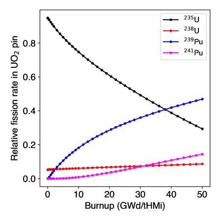
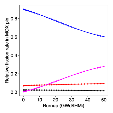
Figure 1: Left: Isotope-specific fractional fission rates for a UO₂ (synonymous with LEU) pin cell, which is equivalent to an MPF of zero. Right: Isotope-specific fractional fission rates for a MOX pin cell, which is equivalent to an MPF of 100%.

2.2 Neutrino Spectral Models

The next step in determining the reactor neutrino flux from a hypothetical reactor is to predict the number of neutrinos emitted per MeV and fission for each of the four primary fissioning isotopes (²³⁵U, ²³⁸U, ²³⁹Pu, and ²⁴¹Pu). There are two types of methods of doing so: the inversion method and the summation method. The inversion method measures the spectrum of electrons emitted from a sample of the fissioning isotope and uses Fermi’s theory of beta decay to calculate the neutrino spectra. This method is limited by the irradiation time of the sample and the precision of the model of beta decay used in the inversion, i.e., whether or not effects such as the emission of photons, weak magnetism, and shape factors are considered in the inversion. The summation method uses data from nuclear databases to sum all of the neutrinos from the relevant beta decays weighted by their activity. It explicitly accounts for each branch of beta decay but is limited by missing information in nuclear databases. In the last decade, the standard has been the Huber-Mueller (HM) model, which uses the inversion method for ²³⁵U, ²³⁹Pu, and ²⁴¹Pu [10], and the summation method for ²³⁸U [11]. The result is the number of neutrinos released per MeV and fission by the four primary fissioning isotopes in the interval 2–8 MeV in bins with a width of 0.25 MeV.

Despite the prevalence of this model, a discrepancy—referred to as the reactor antineutrino anomaly—is observed between neutrino spectra predicted by this model and those observed in experiments [29]. The anomaly is characterized by two features, the rate anomaly, and the spectral bump. The rate anomaly is a discrepancy between the total number of neutrinos observed compared to the prediction from the HM model. Across all reactor neutrino experiments, the ratio of measured to expected neutrinos has been determined to be $0.942\pm 0.009(\text{exp})\pm 0.025(\text{model})$ [6]; in other words, experiments observe $\sim$6% fewer neutrinos than the theoretical models predict. The spectral bump is a measured excess of neutrinos in the energy range from 4–6 MeV. By taking the ratio of the measured neutrino spectra and the expected neutrino spectra, one observes a 4$\sigma$ excess in the range of 4–6 MeV [6]. The observed total neutrino rate is lower than expected, and the observed rate in the 4–6 MeV range is higher than expected, so outside the 4–6 MeV range, the anomaly is greater than a 6% difference.

The discrepancy at lower energies is insignificant for reactor neutrino spectral analysis, although it remains significant in a broader physics context when the total number of neutrinos emitted is important.

Work has been done to improve both methods of determining neutrino spectra. Notably, the Estienne-Fallot model (EF) [12] improved the summation method with the assimilation of newly collected nuclear data into the framework established in the 1950s [30] and continuously improved as more data was made available. The nuclear data previously used by the summation method suffered from the pandemonium effect [31], which resulted in inaccuracies in the neutrino predictions; the EF model used newly collected pandemonium-free data wherever possible. The EF model decreased the expected neutrino rate by approximately 6%, thus matching up with experimental data but exacerbating the significance of the spectral bump. The inversion method was improved by the HKSS model [13] by including corrections for dominant forbidden decays. In the HKSS model, a bump was observed with a similar shape to the spectral bump observed in experimental data, but its amplitude does not fully correlate with experimental observations. The HKSS model additionally predicts an increase in the total neutrino flux by 0.8–2.3%, increasing the significance of the rate anomaly.

A recent new summation technique (PRL2023) simulates beta-transitions with the phenomenological Gamow-Teller decay model, and it accurately accounts for the RAA and the spectral bump [15]. In this study, a free parameter, $\alpha$, is introduced in order to properly renormalize the spectra. This study reports that $\alpha=0.7$ most accurately accounts for the RAA and the spectral bump, and this is the dataset of neutrino spectra we use for ²³⁵U, ²³⁹Pu, and ²⁴¹Pu in conjunction with the HM model’s prediction for ²³⁸U. We use the PRL2023 model’s uncorrelated uncertainties to account for the epistemic uncertainty of the neutrino spectrum. As neutrino models are further improved, their incorporation into this methodology is straightforward.

Although each model predicts different neutrino emission rates, the results are consistent enough to produce similar results for the resolving power of the statistical test. Additionally, across the smallest changes in MPF considered in this study, we find that the difference in neutrino spectra due to the changes in MPF is far greater than differences resulting from uncertainty in the neutrino spectral models. We explore this theoretical model-dependence alongside an experimental model based on RENO collaboration data A.

2.3 Background counts

2.3.1 Antineutrino background

Geoneutrinos and diffuse supernova background (DSNB) comprise non-reactor antineutrino sources in the 2–8 MeV detection energy range [32]. Geoneutrinos originate from radioactive decay in the Earth. Their flux varies geographically within an order of magnitude depending on crustal thickness, radioactivity, and surface heat flux [33]. In contrast, the detected non-neutrino event rate, discussed next, is comparable to the detected reactor neutrino rate, making it the deciding factor in the uncertainties associated with detector measurements in this application. Diffuse supernova neutrino flux is very low compared to reactor flux and nearly constant across the energy range of interest, and it is therefore irrelevant for this analysis. Figure 2 shows the energy-dependent detector counts resulting from these sources integrated over time for a 25 m reactor-detector distance using detector characteristics introduced in Section 2.4. The number of detected reactor neutrino events exceeds the number of detected background neutrinos at the chosen distance of 25 m by a factor of $\sim$10⁷. In fact, the background count is less than 1% of the reactor count up to a distance of 20 km. In the case where the detector is 25 m from the core, it is safe to ignore antineutrino background sources and focus on the primary source of confounding background, the cosmogenic fast neutrons that produce correlated IBD-like detector events. There is a strong motivation to place the neutrino detector as close to the reactor containment building as permitted by intrusiveness considerations so the reactor-originating antineutrino rates overwhelm DSNB and geoneutrinos. Proximity also conveniently decreases the required detector size and cost.

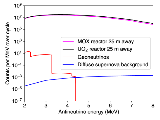
Figure 2: Background antineutrino counts (red, blue) over 50 GWD/tHMi irradiation time in the 2–8 MeV energy range using data from Ref. [32] summed over flavors/masses, compared to the reactor counts (black, magenta).

2.3.2 Non-neutrino detection events

Cosmic rays include muons and hadrons, especially fast neutrons, which can produce detector signals closely resembling antineutrinos. All of these background sources can, in principle, be discerned from true antineutrino events with the degree of discrimination that depends on the event selection criteria (which typically impacts the detection efficiency) and by passive shielding around the detector.

Neutron scattering on hydrogen followed by neutron capture results in two separate events that can mimic those from IBD, with some differences in the energy, time profiles, and topology. We can use these differences to distinguish true antineutrino events as best we can, but it is better to simply allow fewer hadrons to reach the detector. Many neutrino detectors are built underground for this reason, and additional plastic (“low-Z” for low proton number) and heavy metal shielding can be added around the scintillator.

Cosmic ray muons may be captured by nuclei, either inside the detector or in the surroundings, resulting in secondary fast neutrons or pions by $\mu N\to\mu N^{\prime}+X$ inelastic scattering. They may also decay, resulting in another, real electron-flavored antineutrino (that is unlikely to be in the same energy range as from the reactor) and an electron that loses energy into photons similar to the positrons from IBD. Strategic scintillator design, configuration, and data analysis tracks muon paths alongside their scattered hadrons within the detector, allowing for their identification and dismissal from the pool of possible antineutrino-related events; this is often referred to as a muon veto system.

Hadrons resulting from spallation that occurs outside the shielding can hopefully be shielded by the heavy metal surrounding the detector, just like the primary neutron and pion cosmic rays. However, these same shields are rife with nuclei for muons to interact with, producing hadrons that have less shielding to prevent them from reaching the detector. Therefore, neither a muon veto system nor the shields can perfectly prevent their associated background, and there is an optimum amount of shielding that maximizes the background rejection reliability of each.

The simplest way to determine the background rate is to operate the detector in the same conditions (all shielding present, correct location on reactor site, etc.) while the reactor is off. It is also possible to predict non-antineutrino-induced background by using the Monte Carlo simulations of particle interactions in matter, e.g., Fluka [34] and Geant4 [35]. The results will depend on the structure and materials of a particular detector. In this work, we are interested in a general analysis methodology, so making these predictions will be better suited to future work for particular reactor-detector systems. In the current study, total background counts are included as one of the independent variables that determine the probability of discerning a MOX discrepancy. The background count rate can be as high as an order of magnitude above the maximum possible reactor neutrino count rate without selection and shielding, and as low as half of the count rate when we implement the above discernment techniques [36]. Ultimately, the MOX discrepancy determination ability depends on the amount of possible background reduction and on the efficiency of detecting true antineutrino events.

2.4 Neutrino Detection Count Modeling

We model neutrino detection based on a segmented plastic scintillator design similar to the DANSS [36] and PANDA [37] detectors. These detectors are designed to use approximately one ton of scintillator active volume. However, the effectiveness of the methods employed in this study is limited by uncertainties due to counting statistics, and thus larger detectors are necessary to have the sensitivity to provide clear signals of small changes resulting from the diversion of a fraction of the fuel. Therefore, we assume a detector with five tons of plastic scintillator with the characteristics of the EJ-260 [38]—a commercially available plastic scintillator similar to those used in several neutrino detectors, e.g., Ref. [19, 39, 40]. The IAEA has stated that any neutrino detector designed for nonproliferation should be capable of transportation in an ISO container [41]. The volume of this container would be able to fit a 5-ton plastic scintillator detector along with the associated electronics and shielding.

The detected neutrino count collected over time can be modeled by

$$N_{\nu}=\frac{N_{p}}{4\pi D^{2}}\sum_{\ell}\int_{0}^{T}\text{d}t\ N_{\ell}\left(t\right)\int_{1.806\text{ MeV}}^{8\text{ MeV}}\text{d}E\ \sigma\left(E\right)\phi_{\ell}\left(E\right)\epsilon\left(t,E\right).$$ (1)

Here, $N_{\ell}$ is the time-dependent isotope-specific fission rate of nuclide $\ell$ in the hypothetical reactors described in Sect. 2.1. Introduced in Sect. 2.2, $\phi_{\ell}(E)$ is the neutrino emission spectra per fission for nuclide $\ell$. Next, $\sigma(E)$ is the IBD cross-section [42] (Fig. 3) for an electron antineutrino on proton interaction. The detector efficiency $\epsilon$ represents the fraction of IBD events that result in a detected count. The number of free protons in the detector $N_{p}$ is determined by the scintillating material, in this case, the EJ-260 [38]. Lastly, $D$ is the distance between the reactor and the detector, taken to be 25 meters or the approximate distance from the core to the tendon gallery. The energy integral spans from 1.806 MeV, the IBD threshold, to 8 MeV, the maximum energy of the available reactor antineutrino spectral data, and the time integral is applied over the measurement period $T$. The detector efficiency is in general a function of energy, but in this study, we treat it as a constant for simplicity.

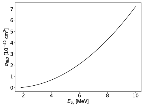
Figure 3: Energy dependent cross section for the process $p+\overline{\nu}_{e}\to e^{+}+n$, also known as inverse beta decay. The cross-section used is a first-order approximation, given as Eq. (11) in Ref. [42]. A first-order approximation is suitable since errors beyond the first order are dominated by the uncertainty in the measurement of the neutron lifetime, which is used to determine the vector and axial vector coupling constants.

To create mock trial data for a reactor with a certain MPF in one-day interval time steps, the neutrino counts are sampled directly from Eq. (1), using the result of the equation as the mean at each time step and assuming a Poissonian variance. Background count rates are assumed to be constant and independent of reactor power, and we treat the rate as a free parameter. When applied to the simulated data, the observed background events are sampled from a normal distribution with a Poissonian variance. We approximate the background rate as a fraction of the average daily neutrino detection rate for a full LEU core. We vary this fraction and explore its effect on the statistical test. Epistemic uncertainties related to the neutrino spectrum model are included but are subdominant compared to statistical fluctuations. Figure 4 shows two examples of sampled mock data using 100% detection efficiency.

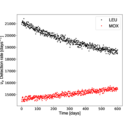
Figure 4: Sample of two trials depicting the number of neutrinos detected each day using a detector with 100% detection efficiency. The trial labeled LEU depicts the results from a core containing entirely low-enriched uranium, while the trial labeled MOX depicts the results from a core containing entirely MOX fuel.

3 Detecting Anomalous Activity

3.1 Test Statistic Formulation

We propose a statistical test in which we compare a quantity $\xi$ between a declared and simulated MOX loading fraction and determine the probability that the measured (simulated) data matches the declared (predicted) expectation. This represents a realistic application of the test in which a reactor operator declares the characteristics of their reactor, and an inspector compares the measured neutrino counts with what is predicted from the declarations and determines the probability of anomalous activity. We define the test statistic $\xi$ as

$$\xi=\frac{n_{1}-n_{2}}{n_{1}+n_{2}-\bar{Y}}.$$ (2)

In this equation, a measurement is taken over a period $\Delta t$; $n_{1}$ represents the number of neutrino counts over the first half of this period, $n_{2}$ represents the number of neutrino counts over the second half, and $\overline{Y}$ represents the expectation of the total number of background counts. This background rate could be measured by inspectors using a neutrino detector while the reactor is offline. This quantity accounts for the total counts and fuel evolution of the entire measuring period, which depends on the power of the reactor and the fuel being used. The left side of fig. 5 shows the time evolution of detected neutrino rate for various MPFs. One can explain the different time-dependencies in this figure by considering the fission rates in Fig. 1 and some known neutrino emission patterns: power from MOX fuel comes primarily from plutonium, which emits fewer antineutrinos with energy above the IBD threshold than LEU fuel at the same power level. Additionally, as MOX fuel is consumed, a smaller fraction of the power is produced by the fission of ²³⁹Pu and more is produced by the fission of ²⁴¹Pu, which, since ²⁴¹Pu emits more antineutrinos per fission than ²³⁹Pu, causes the neutrino emission rate to increase. The opposite is true for LEU fuel: as LEU fuel is consumed, ²³⁵U and ²³⁸U are fissioned and some of the ²³⁸U is transmuted to plutonium through neutron capture and subsequent beta decays. Thus, as time increases, more power is generated from ²³⁹Pu fission, decreasing the neutrino emission rate. The transition between a decreasing and increasing neutrino detection rate occurs when the core consists of around 75% MOX fuel.

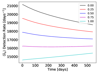
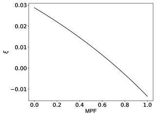
Figure 5: Left: Expected neutrino count rate evolution for various MPFs. A 100% efficient detector is assumed, and Eq. (1) is used in conjunction with the HM model. Right: Expected value of $\xi$ as a function of MPF, computed using Eq. 2 with the HM model, 100% detector efficiency, and zero background over a 540-day observation period.

The quantity $\xi$ trends monotonically with the MPF, shown on the right side of Fig. 5, making it a useful measurement of the amount of MOX fuel in the reactor. It can then be used in a statistical test to determine if a measured value, using data similar to Fig. 4, matches with a predicted value, using data similar to Fig. 5. The statistical significance of the difference between the measured and predicted value can be quantified by the uncertainty in the predicted value, and a $p$-value can be determined, indicating the probability of compatibility between the two values.

3.2 Test Statistic Uncertainty Propagation

Throughout this study, there are many sources of uncertainty to account for. The aleatory (statistical) uncertainty is straightforwardly Poissonian because of the random timing of the fissions that originate the neutrinos. The most significant epistemic uncertainties (systematic unknowns) originate from the neutronics simulation and the neutrino spectral models. Aside from the negligible time-dependent, isotope-specific uncertainties in fission reaction rates reported by the Monte Carlo neutron transport calculation method associated with the Serpent 2 neutronics code, there are also uncertainties in cross sections within the nuclear libraries used for the simulation. Reference [43] computationally propagates the cross-section covariance data through burnup to determine the effect on isotopic composition after a burnup of 50 GWD/MTHM. The coefficient of variation describing the uncertainty distribution in isotopic composition can also describe the uncertainty distribution in the fission rate. To construct a burnup-dependent uncertainty we assume the cross-section uncertainty starts at zero at 0 GWD/MTHM and increases linearly to match the 50 GWD/MTHM uncertainty reported in Ref. [43]. The total uncertainty of the fission rates is propagated as an epistemic source of error through the neutrino count model in Eq. (1).

The PRL2023 neutrino spectral model’s discrepancy from the true neutrino spectrum is quantified by uncorrelated energy-dependent, isotope-specific uncertainties. We take a Monte Carlo approach to determine the resulting systematic variance in detected neutrino counts.

After separately determining all of these time-dependent contributions to the variance of the neutrino detection rate, they can be added in quadrature to find the total uncertainty in $n_{1}$ and $n_{2}$,

$$\sigma_{n_{i}} =\sqrt{{\sigma^{2}_{n_{i}}}_{\text{systematic}}+{\sigma^{2}_{n_{i}}}_{\text{statistical}}}$$ (3)

$$=\sqrt{{\sigma^{2}_{n_{i}}}_{\text{systematic}}+{n_{i}}_{\text{declared}}}$$ (4)

Similarly, we use the more general error-propagating approximation

$$\sigma_{\xi_{\text{declared}}}=\sqrt{\left|\dfrac{\partial\xi}{\partial n_{1}}\right|^{2}\sigma_{n_{1}}^{2}+\left|\dfrac{\partial\xi}{\partial n_{2}}\right|^{2}\sigma_{n_{2}}^{2}}$$ (5)

to find the standard deviation of $\xi$ used in the statistical test described previously. There are additional possible sources of uncertainty unique to each deployment, i.e., detector size, efficiency, reactor power levels, and fuel enrichment. These uncertainties can be propagated through nuclear transport codes or appear as additional terms in Eq. (3).

3.3 Detection of Anomalous Fuel Loading

This test is designed to detect anomalous fuel loading in nuclear reactors partially loaded with MOX fuel. The enrichment process and production of weapons-grade plutonium are not the primary concern of this study. Instead, we are concerned with the diversion from a reactor of fresh MOX fuel with a plutonium content that would be considered weapons-grade. We model this diversion scenario using the method described in Sect. 2.1. Diversion results in a discrepancy in neutrino count rate evolution from our expected counts, which our statistical test is capable of observing. We quantify this method’s resolving power in Sect. 4.1.

As a demonstration of how this statistical test functions, consider the following case. A reactor facility declares the enrichment, quantity, and positional distribution of fuel within a partially loaded MOX core. These declarations are simulated using a high-fidelity nuclear transport code, and the MPF for these declarations is found to be 0.25. With the reactor model used in this study, this means that 25% of the total fuel in the reactor is MOX. In a more realistic reactor model, there are several different configurations of fuel distribution, enrichment, and quantity of MOX fuel that could lead to this. It’s worth noting that an ill-intentioned rector operator may divert some of the MOX fuel, and redistribute the fuel within the reactor to produce the same MPF, but with less MOX fuel. However, this would still be detectable as to produce the same MPF, the MOX fuel would have to be burned up quicker, thus producing more energy from ²⁴¹Pu and ²³⁸U, which would be detectable with our methodology. The isotope-specific time-dependent fission fractions determined by the simulation are used in Eq. (1), along with the HM spectral model and detector material and size, to determine the expected neutrino detection rate. With this rate, the expected value of $\xi_{\text{declared}}$ is determined for a total observation period of 540 days, approximately 18 months, or the typical operation time of a reactor between refueling. Meanwhile, suppose the reactor operator chooses to divert 12% of the MOX fuel supplied to them to a nuclear weapons program, corresponding to about 120 kg of WGPu. This implies that their fuel would burn up more quickly in order to maintain the same power output. In an attempt to avoid detection, the MOX fuel is replaced with LEU fuel, to ensure the power output is consistent. With this new fuel configuration, the MOX power fraction has changed to an MPF of 0.22. The reactor operates under these conditions for the duration of the measurement period. Figure 6 depicts the number of neutrinos measured each day during the observation period, as well as the number expected from the declared MPF of 0.25.

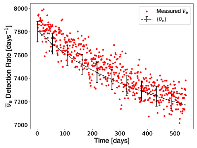
Figure 6: Simulated measurement of the neutrino count rate for a reactor with an MPF of 0.22 for a 540-day observation period corresponding to the true core (red), and the expected count rate and associated uncertainty for a reactor with an MPF of 0.25 corresponding to the declared core (black). This scenario corresponds to a neutrino detector with a 40% detector efficiency.

For configurations with enough discrepancy between declared and implemented MPF, the difference between expected neutrino counts and observed neutrino counts is qualitatively inconsistent. However, in this case, where very little MOX fuel is diverted, depicted in Fig. 6, it is difficult to observe a significant difference by eye, necessitating this precise statistical test.

For each of these trial sets of data, $\xi$ is calculated and compared using

$$z=\frac{\xi_{\text{measured}}-\xi_{\text{declared}}}{\sigma_{\xi_{\text{declared}}}}.$$ (6)

In this study, $\xi_{\text{measured}}$ is a Gaussian distributed random variable, but in the real-life procedure it is measured from the observed antineutrino counts each day according to eq. 2. The total (epistemic and aleatory) predicted uncertainty $\sigma_{\xi_{\text{declared}}}$ from eq. 5. We determine a $p$-value assuming that $\xi_{\text{declared}}$ is Gaussian-distributed; indeed, $\sigma_{\xi_{\text{declared}}}$ ends up being dominated by statistical uncertainty, and the systematic variance results from Gaussian sampling. We use $\alpha$-levels 0.05 and 0.01.

In our example case, eq. 6 gives $z=2.45$, corresponding to a $p$-value of $\approx 0.014$; we can determine that the difference between reactor operations and declarations is statistically significant, even for such a small MPF divergence. In this study, we simulate reactors with measured MPFs lower than the declared to determine our sensitivity to the diversion of fresh MOX fuel, corresponding to an illegitimate removal of weapons-grade plutonium.

4 Results

4.1 Quantification of Discriminatory Power

We visualize the resolving power of the statistical test using a contour plot depicted in fig. 7. In these plots, each pixel represents $N$ statistical tests, the $x$-axis represents the simulated measured MOX power fraction, the $y$-axis represents the MOX power fraction declared by the operators of a safeguarded reactor, and the color represents the fraction of trials in which the declared and measured MPF are distinguished at the 95% confidence level.

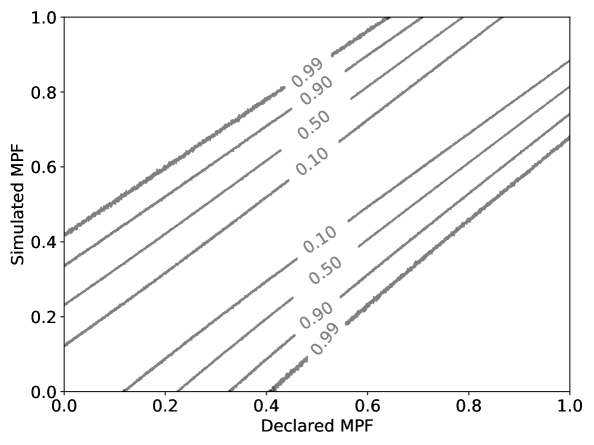
Figure 7: Fractions of $10^{4}$ trials that successfully distinguish declared and true MPF at the 95% confidence interval using a detector with 20% efficiency. Here we assume 30% background and use the HM model to calculate the expected neutrino count.

The information in the contour plot can be reduced to a line, like in fig. 8, by establishing a threshold $f$ of the fraction of trials where the declared and measured MPF are distinguished at the 95% confidence level. This line plot represents the difference between declared and measured MOX power fraction of which can be distinguished in $f=90\%$ of trials (corresponding to the contour at 0.9), providing an MPF “resolution” as a function of declared MPF that can be compared. Since we are primarily concerned with the diversion of fresh MOX fuel, this is specifically the distance between the lower 90% contour in fig. 7 and the identity line (the contours are not symmetric across it). From the assumption that each fuel rod in the reactor is producing equivalent power, this core fraction is related to the mass of weapons-grade plutonium diverted by a constant multiplicative factor that can be determined using fuel rod characteristics from [24]. Note that the $x$-axis for these plots starts at an MPF different from 0, since at MPFs less than this, no diversion can be detected for this scenario. we use plots such as these to quantify our power to discriminate between two reactors with different fuel loadings. Thus our discriminatory power can be quantified by the inverse of the minimum detectable diversion for a given pair of MPFs, detector, and observation period, i.e. if we can detect a smaller diversion, our discriminatory power is greater.

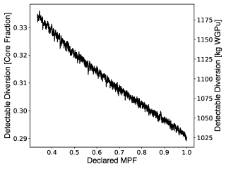
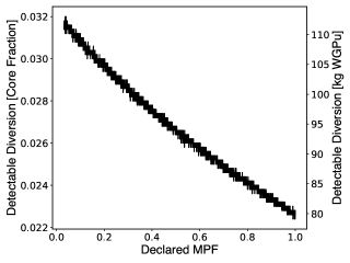
Figure 8: Minimum divertible core fraction and plutonium mass that can be detected in 90% of trials. Left: detector with 20% efficiency, 30% background, and for a relatively short measurement period of 180 days. Right: detector with 100% efficiency, no background and a measurement period of 18 months (540 days).

4.2 Effect of Detector Efficiency

We would like to explore the sensitivity of our statistical test to detector efficiency, which ranges from about 5% to near 50% in modern neutrino detectors [40, 44]. We generate diversion line plots for several different detector efficiencies in fig. 9. For each line shown, the underlying test assumes a zero background rate, a 180-day measurement period, and data is produced using both the PRL2023 and HM models. As one might expect, a lower efficiency leads to a less sensitive measurement because fewer detected events mean a lower difference between neighboring MPFs. What is less intuitive is the dependence of the discriminatory power on the declared MPF. In fig. 9, the slope of these lines is steeper for lower efficiencies—with lower efficiency, the difference in discriminatory power between a low declared MPF and a large declared MPF is greater than for higher efficiency. These slope differences result from the variation in uncertainty between MPFs.

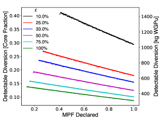
Figure 9: Minimum divertible core fraction and plutonium mass that can be detected in 90% of $10^{4}$ trials for various detector efficiencies. Each test uses an observation period of 180 days and no background. The two sides show results using the HM model (left) and the PRL2023 model (right).

To further quantify efficiency-dependent and MPF-dependent effects on discriminatory power, we analyze 100 different values ranging from 0.01 and 1. The minimum detectable diversion as a function of efficiency is shown in fig. 10 for two specific declared MPFs. As expected, the discriminatory power is proportional to the number of events observed.

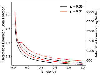
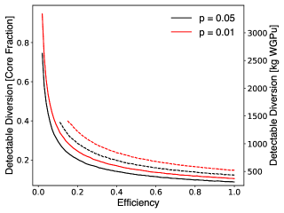
Figure 10: Minimum divertible core fraction and plutonium mass that can be detected in 90% of $10^{4}$ trials depending on detector efficiency. The two sides show data produced using the HM model (left) and the PRL2023 model (right). The declared MPFs are 0.4 (dashed) and 1 (solid).

4.3 Effect of Background

Next, we explore the effect of different background rates. We treat the background as a rate sampled on each day from a Gaussian distribution with a coefficient of variation of unity. We assume a detector with a 20% detector efficiency and use an observation period of 180 days. Neutrino count rates are produced using both the PRL2023 and HM models. To determine a background rate we vary a percentage of the average neutrino detection rate over the observation period for a reactor with an MPF of 0, or a total LEU core. Reactor neutrino detectors have reported signal-to-background ratios ranging from 0.2 to 1 [45].

Figure 11 shows the line plot of minimum detectable diversion as a function of MPF for several background rates. Naturally, a higher background rate leads to a worse discriminatory power because of the increased statistical uncertainty and a smaller change in the count rate with observation time. Figure 12 depicts minimum detectable diversion for 100 different background rates.

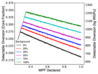
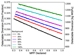
Figure 11: Minimum divertible core fraction and plutonium mass that can be detected in 90% of $10^{4}$ trials for various background rates. Each test uses a detector efficiency of 20% over an observation period of 180 days. The two sides show data produced using the HM model (left) and the PRL2023 model (right).

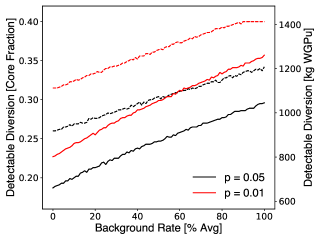
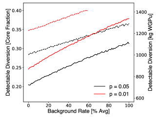
Figure 12: Minimum divertible core fraction and plutonium mass that can be detected in 90% of $10^{5}$ trials depending on background rate.The two sides show data produced using the HM model (left) and the PRL2023 model (right). The declared MPFs are 0.4 (dashed) and 1 (solid).

4.4 Application to Continuous Monitoring

Next, we explore the effect of different observation periods. We use a detector with a 20% detector efficiency and no background. Neutrino count rates are produced using the PRL2023 model. We explore observation periods ranging from 45 days to 540 days; five hundred and forty days is the average amount of time between the two reactor refuelings.

Figure 13 shows the results for several different observation periods. With an observation period of 45 days, more than half of the core could be diverted without our test distinguishing it. However, for a longer measurement period, the discriminatory power improves: for a measurement period of 540 days, the test can distinguish between reactors with a 7% difference in fuel loading. For reactors with different MPFs the neutrino count rate evolution is different for all times, so longer observation periods increase the difference in our test statistic for different fuels. Figure 14 shows the relationship between the maximum of the line plots and the measurement period. We explored 100 different values of $\Delta t$ ranging from 6 days to 600 days. The divertable core fraction is indeed inversely proportional to the length of the observation period. The $p=0.01$ curve in fig. 14 is only slightly higher than the $p=0.05$ curve, implying that a confidence level above the 95% threshold may be reasonably achievable for many deployments.

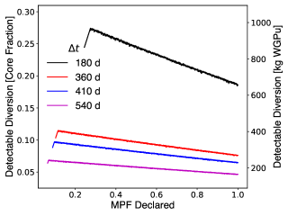
Figure 13: Minimum divertible core fraction and plutonium mass that can be detected in 90% of $10^{4}$ trials. Each test uses a detector efficiency of 20% and no background. The two sides show data produced using the HM model (left) and the PRL2023 model (right).

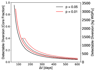
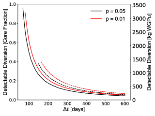
Figure 14: Minimum divertible core fraction and plutonium mass that can be detected in 90% of $10^{4}$ trials depending on observation period. The two sides show data produced using the HM model (left) and the PRL2023 model (right). The declared MPFs are 0.4 (dashed) and 1 (solid).

We can see in figs. 10, 12 and 14 that lower background, higher efficiency, and longer observation times lead to a higher discriminatory power. We find that increasing efficiency leads to diminishing returns, while the effect of reducing background is linear. However, this trade-off is deployment specific—the slopes of the lines in fig. 12 depend on the declared MPF (steeper for larger MPFs), and practical background reduction techniques may have higher order effects (e.g. harsher energy cuts leading to a lower neutrino detection rate).

5 Conclusion

We have presented a simple observable and associated statistical test to determine possible plutonium diversion from fuel intended for nuclear reactor operation. The method relies on measuring the fraction of MOX fuel present in a reactor by using an antineutrino detector near a commercial power reactor partially loaded with MOX fuel. To this end, we generated time-dependent, isotope-specific fission rates using the Serpent neutronics code base to model pin cells with different fuels and used a weighted sum to determine the fission rates for an entire reactor with a given fraction of MOX fuel. We then compared reactors with different initial fuel loadings using the straightforward statistical test we developed.

The presented statistical test contains information not only on the absolute rate of neutrino observations but also on the neutrino count rate evolution. Both of these attributes of the reactor neutrino emissions are useful in characterizing the amount of plutonium in a reactor due to the differences in the neutrino emissions of the four primary fissioning isotopes and the difference in fuel evolution between MOX fuel and LEU fuel.

The presented statistical test considers both the Monte Carlo and the cross-section uncertainty. In optimal conditions, i.e., zero background, 100% detector efficiency, and 540-day observation period, this method is capable of signaling the removal of as little as 80 kg of weapons-grade plutonium with a detector containing 5 tons of liquid scintillator placed 25 m from the reactor core.

The IAEA has a stated goal to be able to determine the diversion of a single significant quantity (8 kg of plutonium containing less than 80% of ²³⁸Pu) of plutonium in 90 days. The method as described here does not reach that ultimate goal but has demonstrated improved sensitivity in some cases [46, 8]. In the future we can combine our new statistical test with other techniques, notably spectral analysis, to compound the sensitivity of MOX diversion detection and achieve the IAEA target.

In addition to exploring the capabilities of this statistical test, we also explored the impact of neutrino spectral models released in light of the reactor neutrino anomalies and the sensitivity of our statistical test to various parameters such as detector efficiency, background rates, and different durations of observation. We found that the results varied insignificantly between the HKSS model, the HM model, and a model created using experimental observations of the RENO collaboration. The EF model predicts the neutrino spectra of ²³⁹Pu and ²³⁵U to be similar, which, compared to other models, would decrease the ability to distinguish between MPFs. The PRL2023 model, which is the latest model set and the one we primarily used in this analysis, gives results similar to those of EF at lower MPF and similar to those of the other models at higher MPF. Furthermore, as one would expect, decreasing detector efficiency, increasing background rates, and decreasing the duration of the observation period lessens the ability of our statistical test to distinguish between reactors with different fuel loading and thus the diversion of fresh MOX fuel and WGPu.

We have demonstrated that this rate-based neutrino measurement has applications for estimating reactor fuel composition and can be useful within a semi-cooperative framework to determine anomalous activity. One hurdle for improving our method is a better determination of the time-dependent, isotope-specific fission rates. Any improvements would need to be done using a high-fidelity neutronics model that factors in the complexity of an assembly-level simulation as well as the complexity of fuel shuffling throughout the fuel cycle. Despite the challenges such a measurement has, the method demonstrates the potential utility of reactor safeguarding using neutrino detectors.

6 Acknowledgments

This work was partially supported by the Department of Energy National Nuclear Security Administration, Consortium for Monitoring, Verification and Technology (DE-NE000863). JW would like to thank N.S. Bowden for discussions and the Center for Global Security Research (CGSR) at Lawrence Livermore Laboratory for residency during parts of the research of this publication. Also, this material is based on work supported under a Department of Energy, Office of Nuclear Energy, Integrated University Program Graduate Fellowship.

Appendix A Dependence on Neutrino Spectral Model

The standard neutrino spectral model has been the Huber-Mueller model[10, 11] for the last decade, but this model does not accurately account for all of the observed features in the neutrino spectra. The two discrepancies, the reactor neutrino anomaly, and the 4–6 MeV spectral bump, have been an issue since their discovery. Several revised models have since been published. Here we explore the implications of five different models: four from theory, and one from experiment. The four theoretical neutrino spectral models considered are the PRL2023 model [15], the Huber-Mueller model [10, 11], the HKSS model [13], and the Esteinne-Fallot (EF) Model [12]. A 2019 paper from the RENO collaboration published [47] in the context of the reactor neutrino anomaly also provided their measured IBD yield for each of the four primary fissioning isotopes; the IBD yield is the energy integral in eq. 1. Figure 15 depicts the resolution as a function of declared MPF for each of the neutrino spectral models. For each line, the scenario simulated is 20% efficiency, no background, and an observation period of 180 days. For the EF, HKSS, and HM models, the reported uncertainties are fully correlated across all energies and isotopes and the correlation matrices are not published. For this reason, the uncertainties associated with these models are treated as zero. For the Reno and PRL2023 models, each source published uncorrelated uncertainties that could easily be propagated through standard techniques, so we can include them in the statistical test. These uncertainties make an extremely subdominant contribution to the total uncertainty, so the inclusion of these uncertainties has virtually no impact on the comparative performance of these models in this study.

As is evident in fig. 15, the model using data from the RENO collaboration, the HKSS model, and the HM model all produce very similar results. The EF model consistently produces a lower discriminatory power. The PRL2023 model produces a discriminatory power similar to EF at low MPF while the discriminatory power at higher MPF is in between the HM and EF models. The variations from the EF model can be explained by the nature of our measurement—the primary difference between different neutrino emission rates of reactors with different fuel is the fission rates of ²³⁵U and ²³⁹Pu. In LEU pins, most of power comes from the fission of ²³⁵U while in MOX pins, most of the power comes from ²³⁹Pu. If a neutrino model predicts the IBD yield from ²³⁵U and ²³⁹Pu to be similar, then the difference in neutrino measurements between MPFs with this model would be small. This is exactly the case with the EF model. The ratio of the IBD yields of ²³⁵U and ²³⁹Pu for the HM model is $\approx 1.527$, $\approx 1.525$ for the HKSS model, $\approx 1.529$ for the model using data from RENO, $\approx 1.428$ for the EF model. The fact that the EF model’s ratio is closer to unity means that it is more difficult to distinguish between LEU fuel and MOX fuel as we see in fig. 15.

The PRL2023 model’s differences can be explained by a similar nature. The PRL2023 model matches well with the EF model for the ratio ²³⁵U and ²³⁹Pu explaining the similarity at low MPF; however, there is a qualitative difference in the predictions for ²⁴¹Pu, leading to the differences observed at higher MPF. The PRL2023 data reports uncorrelated uncertainties, which we include in our statistical test. Taking these uncertainties into account slightly reduces the discriminatory power relative to the statistical test results we obtained using the other models.

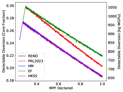
Figure 15: Line plots depict diversion that can be determined 90% of the time. The $x$-axis represents the declared MPF, and the $y$-axis represents the fraction of the core/mass WGPu that can be diverted. Each test represents an observation period of 180 days, 20% detector efficiency, and no background. $10^{4}$ tests were completed for each pair of declared and simulated MPF, with an MPF precision of 1/5000. Each line represents a different method of predicting the number of neutrinos measured each day: the four neutrino spectral models and one data-driven model.